KA-TP-07-2007

Linear growth of the trace anomaly in Yang-Mills thermodynamics

Francesco Giacosa^† and Ralf Hofmann^∗

$\mbox{}^{\dagger}$ Institut für Theoretische Physik
Universität Frankfurt
Johann Wolfgang Goethe - Universität
Max von Laue–Str. 1
60438 Frankfurt, Germany

$\mbox{}^{*}$ Institut für Theoretische Physik
Universität Karlsruhe (TH)
Kaiserstr. 12
76131 Karlsruhe, Germany

In the lattice work by Miller [1, 2] and in the work by Zwanziger [3] a linear growth of the trace anomaly for high temperatures was found in pure SU(2) and SU(3) Yang-Mills theories. These results show the remarkable property that the corresponding systems are strong interacting even at high temperatures. We show that within an analytical approach to Yang-Mills thermodynamics this linear rise is obtained and is directly connected to the presence of a temperature-dependent ground state, which describes (part of) the nonperturbative nature of the Yang-Mills system. Our predictions are in approximate agreement with [1, 2, 3].

1 Introduction

Studies of pure SU(2) and SU(3) Yang-Mills theories at finite temperature $T$ represent an important subject in modern high energy physics and a fundamental step toward the analysis of the properties of the Quark-Gluon-Plasma. In particular, the question if and for which temperatures a gas of (almost) free gluons offers a valid approximate description of such strong interacting theories goes to the heart of the problem. A key-quantity to address this issue is the trace of the stress energy tensor $\theta_{\mu\mu}\equiv\rho-3p,$ where $\rho$ and $p$ are the energy density and the pressure of the system. In fact, the trace $\theta_{\mu\mu}$ vanishes for a free gas of massless gluons, being a consequence of conformal invariance of Yang-Mills theories. Thus, one would expect that $\theta_{\mu\mu}$ vanishes in the high-temeperature limit, where a Yang-Mills theory is asymptotically free.

In the lattice simulations of Refs. [1, 2, 4], based on the lattice works of Refs. [5], a striking result was found: the trace of the stress-energy tensor $\theta_{\mu\mu}\equiv\rho-3p$ of pure SU(2) and SU(3) Yang-Mills thermodynamics in the deconfining phase does $not$ vanish (and neither decreases) but $grows$ linearly with $T$ for $T\gtrsim 2\,T_{c}$ where $T_{c}$ denotes the phase boundary. As emphasized in [1], this result means that the system is strong interacting even at high $T$ and puts strong constraints on models aiming at describing these Yang-Mills theories at finite $T$. Notice that in [6] a quadratic rise at high $T$ (instead of linear) of $\theta_{\mu\mu}$ is inferred out of lattice data in the SU(3) case. On one hand this difference points to the difficulty in extracting high $T$ behavior for thermodynamical quantities, on the other hand it confirms that nonperturative physics is at work in the high temperature domain.

While phenomenological models [7, 8, 9] predict that, in accord with asymptotic freedom [10], the interaction measure $\Delta=\frac{\rho-3p}{T^{4}}$ vanishes for $T\rightarrow\infty$, there is no general agreement on how fast $\Delta$ approaches zero. Namely, as discussed above, not only $\Delta$ but the quantity $\rho-3p$ itself should vanish for $T\rightarrow\infty$ if the thermodynamical system is described by a noninteracting realtivistic gas of gluons. Notice that in the framework of resummed perturbation theory nonzero contributions to $\theta_{\mu\mu}$ start at order $g^{4}$ [11], where it is shown that $\theta_{\mu\mu}$ keeps growing even for high $T.$

Assuming the correctness of the results of [1], it is therefore important to study models which $do$ describe the linear growth of $\theta_{\mu\mu}$ in order to understand the origin of this property. In this work we show that within the analytical approach to Yang-Mills thermodynamics of Ref. [12] the linear growth of $\rho-3p$ is predicted with slopes compatible with lattice results. This property is a consequence of the presence of a thermal ground state, which takes into account the contributions of calorons (i.e. instantons at finite $T$). Intuitively, this thermal ground state, described by an adjoint-scalar field $\phi$, represents an $average$ over such topologically non-trivial configurations. From a phenomenological perspective the ground-state contribution to $\rho$ behaves like a temperature dependent bag constant, see for example [7]. Furthermore, the introduced field $\phi$ generates a Higgs mechanism: (some of) the gauge modes acquire a temperature-dependent mass, see details in following Section.

The ground-state contribution to the pressure $p_{gs}$ is negative (like the bag pressure is) and dominates when $T\searrow T_{c}$. Lattice simulations of $p$ do not agree on this point. Namely, within the differential method, close to $T_{c}$ negative pressure is predicted [13] while the integral method [14] is designed to generate positive pressure. However, in the present report we investigate $\theta_{\mu\mu}$ only for $T\gtrsim 1.5\,T_{c}$, thus well above the phase boundary.

In Ref. [3] a linear growth of $\theta_{\mu\mu}$ was obtained based on the suppression of the infrared modes by invoking a modified dispersion relation of Gribov type. The latter circumvents the well-known problems inherent in a perturbative treatment [15]. In the alternative approach of [12, 16, 17, 18] the stability of the infrared sector is guaranteed by the above mentioned thermal ground state, embodied by an adjoint scalar field $\phi$, taking into account nontrivial-topology fluctuations. Remarkably, this approach predicts the slopes $\alpha$ in $\theta_{\mu\mu}=\alpha T$ once the Yang-Mills scale $\Lambda$ (or alternatively $T_{c}$) is fixed.

The present analysis is not intended to discuss phenomenological fits to lattice curves (for work in that respect see [7, 9, 8] and the review [19]). Rather, our goal is to show that the (asymptotically) linear growth of $\theta_{\mu\mu}$ is related to the presence of a nontrivial and temperature-dependent ground-state [12, 16].

The paper is organized as follows: First we briefly review the approach of Ref. [12] and list expressions for $\rho$ and $p$ in the SU(2) case. Subsequently, we show numerically and analytically that within this approach $\theta_{\mu\mu}=\alpha T$ for $T\gg T_{c}$ and compare $\alpha$ with the results of [1, 2, 3]. We then discuss the SU(3) case and give our conclusions.

2  The SU(2) case

 In Ref. [12] an adjoint scalar field $\phi$ is derived which, upon spatial coarse graining, describes the dynamics of nontrivial, BPS-saturated topological configurations [20, 21] giving rise to an energy density and pressure of the thermal ground state. The field $\phi$ acts as a background to the dynamics of topologically trivial fluctuations.

The modulus $\left|\phi\right|=\sqrt{\frac{\Lambda^{3}}{2\pi\,T}}$ exhibits a dependence on $T$ and on $\Lambda$. The corresponding potential is $V(|\phi|^{2})=\Lambda^{6}/|\phi|^{2}$ [12, 16]. In unitary gauge the effective Lagrangian describing a thermalized, pure SU(2) Yang-Mills system reads:

$$\mathcal{L}_{{\tiny\mbox{eff}}}^{u.g.}=\mathcal{L}\left[a_{\mu}\right]=\frac{1}{4}\left(G_{E}^{a,\mu\nu}[a_{\mu}]\right)^{2}+2e^{2}\left|\phi\right|^{2}\left(\left(a_{\mu}^{1}\right)^{2}+\left(a_{\mu}^{2}\right)^{2}\right)+2\frac{\Lambda^{6}}{\left|\phi\right|^{2}}\,,$$ (1)

where $e=e(T)$ denotes the temperature dependent effective gauge coupling (see below) which enters both into the effective field strength $G_{E}^{a,\mu\nu}$ and into the mass $m$ for the fields $a_{\mu}^{1,2}$. One has

$$m^{2}=m(T)^{2}=m_{1}^{2}=m_{2}^{2}=4e^{2}\left|\phi\right|^{2}\,,\ \ \ \ m_{3}^{2}=0\,.$$ (2)

that is a temperature-dependent mass is generated in a nonperturbative fashion by the adjoint-scalar field $\phi.$ From the effective Lagrangian (1) one derives, on the one-loop level (accurate to about 0.1% [18, 22]), the energy density $\rho$ and the pressure $p$ as

$$\rho=\rho_{3}+\rho_{1,2}+\rho_{gs}\,,\ \ \text{ }p=p_{3}+p_{1,2}+p_{gs}\,,$$ (3)

where $\rho_{1,2}$ denotes the sum over the two massive modes. Explicitly we have:

$$\rho_{3} = 2\,\frac{\pi^{2}}{30}\,T^{4},\text{ }\rho_{1,2}=6\,\int_{0}^{\infty}\frac{dk\,k^{2}}{2\pi^{2}}\frac{\sqrt{m^{2}+k^{2}}}{\exp(\frac{\sqrt{m^{2}+k^{2}}}{T})-1},\text{ }\rho_{gs}=2\frac{\Lambda^{6}}{\left|\phi\right|^{2}}=4\pi\Lambda^{3}T\,.$$ (4)

$$p_{3} = 2\frac{\pi^{2}}{90}T^{4},\text{ }p_{1,2}=-6\,T\int_{0}^{\infty}\frac{dk\,k^{2}}{2\pi^{2}}\ln\left(1-e^{-\frac{\sqrt{m^{2}+k^{2}}}{T}}\right)\,,\text{ }p_{gs}=-\rho_{gs}\,.$$ (5)

Let us now rewrite the system in terms of dimensionless quantities:

$$\overline{\rho}=\frac{\rho}{T^{4}},\text{ }\ \overline{p}=\frac{p}{T^{4}},\text{ }\ \lambda=\frac{2\pi T}{\Lambda},\text{ }\ a(\lambda)=\frac{m(T)}{T}=2\frac{e(T)}{T}\left|\phi\right|\,,$$ (6)

where the function $a=a(\lambda)$ is introduced for later use. In dependence of the dimensionless temperature $\lambda$ the dimensionless energy density $\bar{\rho}$ and pressure $\bar{p}$ read:

$$\overline{\rho}_{3}=2\,\frac{\pi^{2}}{30}\,,\text{ }\overline{\rho}_{1,2}=\frac{3}{\pi^{2}}\int_{0}^{\infty}dx\,\frac{x^{2}\sqrt{x^{2}+a^{2}}}{e^{\sqrt{x^{2}+a^{2}}}-1}\,,\text{ }\overline{\rho}_{gs}=\frac{2(2\pi)^{4}}{\lambda^{3}}\,,$$ (7)

$$\overline{p}_{3}=2\,\frac{\pi^{2}}{90}\,,\ \text{ }\overline{p}_{1,2}=-\frac{3}{\pi^{2}}\int_{0}^{\infty}dx\,x^{2}\ln\left(1-e^{-\sqrt{x^{2}+a^{2}}}\right)\,,\ \text{ }\overline{p}_{gs}=-\text{ }\overline{\rho}_{gs}\,.$$ (8)

By virtue of the Legendre transformation

$$\rho=T\frac{dP}{dT}-P\iff\overline{\rho}=\lambda\frac{d\overline{p}}{d\lambda}+3\overline{p}$$ (9)

the evolution equation for $a=a(\lambda)$ follows:

$$1 = -\frac{6\lambda^{3}}{(2\pi)^{6}}\left(\lambda\frac{da}{d\lambda}+a\right)aD(a),\text{ }$$ (10)

$$D(a) = \int_{0}^{\infty}dx\frac{x^{2}}{\sqrt{x^{2}+a^{2}}}\frac{1}{e^{\sqrt{x^{2}+a^{2}}}-1},\text{ }a(\lambda_{in})\ll 1.$$ (11)

There exits a low-temperature attractor to the evolution described by Eq. (10) with a logarithmic pole at the critical temperature $\lambda_{c}=13.89$ [12]. At $\lambda_{c}$ the fluctuations $a_{\mu}^{1,2}$ decouple thermodynamically. The effective coupling is given as $e=e(\lambda)=a(\lambda)\lambda^{3/2}/4\pi$. For $a\ll 1$ the coupling $e$ is constant: $e=\sqrt{8}\pi$. In fact

$$a(\lambda)=\frac{8\sqrt{2}\pi^{2}}{\lambda^{3/2}}$$ (12)

then is a solution to Eq. (10). This plateau is reached rapidly for increasing $\lambda$, see figures in [12].

3  Linear growth of $\theta_{\mu\mu}$

We now turn to the linear rise of $\theta_{\mu\mu}$ within the approach described in the previous Section. In therms of dimensionless quantities one has

$$\frac{\theta_{\mu\mu}}{\Lambda^{4}}=\frac{\rho-3p}{\Lambda^{4}}=\left(\frac{\lambda}{2\pi}\right)^{4}(\overline{\rho}-3\overline{p})\,.$$ (13)

A plot of the quantity $\frac{\theta_{\mu\mu}}{\Lambda^{4}}$ is shown in Fig. 2. Notice the linear growth.

Figure 1: The quantities $\frac{\theta_{\mu\mu}}{\Lambda^{4}}$ (left panel, gray curve: large-$T$ behavior; black curve: finite-$T$ behavior) and $h$ (right panel) as functions of $\frac{\lambda}{\lambda_{c}}=\frac{T}{T_{c}}$ in the case of SU(2).

Asymptotically ($\lambda\gg\lambda_{c}$) this linear rise can be shown to hold analytically. To this end let us consider the function

$$h(\lambda)=\frac{\rho-3p}{4\rho_{gs}}=\frac{\overline{\rho}-3\overline{p}}{4\overline{\rho}_{gs}}=1+\frac{\overline{\rho}_{1,2}-3\overline{p}_{1,2}}{4\overline{\rho}_{gs}}\,.$$ (14)

For $a\ll 1$ (i.e. $\lambda\gg\lambda_{c}$) we have [23]:

$$\overline{\rho}_{1,2}=6\,\frac{\pi^{2}}{30}-\frac{1}{4}a^{2}+\cdots,\text{ }\overline{p}_{1,2}=6\,\frac{\pi^{2}}{90}-\frac{1}{4}a^{2}+\cdots\,.$$ (15)

As a consequence, the function $h=h(\lambda)$ becomes:

$$h(\lambda)=1+\frac{\frac{1}{2}\,a^{2}}{4\frac{2(2\pi)^{4}}{\lambda^{3}}}+\cdots=1+\frac{\lambda^{3}a^{2}}{16(2\pi)^{4}}+\cdots=\frac{3}{2}+\cdots\,,$$ (16)

where Eq. (12) has been used. Thus $h(\lambda)$ is approximately constant for $a\ll 1$. The numerical behavior for the function $h=h(\lambda)$ is plotted in the right panel of Fig. 1. Notice that the asymptotic value $h(\lambda)\equiv\frac{3}{2}$ is practically reached for $\lambda\geq 5\,\lambda_{c}$.

By virtue of Eq. (14) we have asymptotically (corresponding to the gray curve in the left panel of Fig 1):

$$\rho-3p=6\rho_{gs}=24\pi\Lambda^{3}T\,.$$ (17)

It is interesting that $\theta_{\mu\mu}$ splits as $\theta_{\mu\mu}=6\rho_{gs}=4\rho_{gs}+2\rho_{gs}$ where the first summand is the direct contribution of the ground state while the second summand arises from the massive modes $a_{\mu}^{1,2}$. That is, the mass $m=m(T)$ behaves in such a way that fluctuations generate a linear contribution to $\theta_{\mu\mu}$ at high $T$.

Let us now compare our prediction for the slope with lattice results. To this end we relate the Yang-Mills scale $\Lambda$ to the critical temperature $T_{c}$ as

$$\Lambda=\frac{2\pi T_{c}}{\lambda_{c}}\simeq 0.45\,T_{c}\,,$$ (18)

where $\lambda_{c}=13.89$ has been used. Then we have asymptotically

$$\theta_{\mu\mu}=\rho-3p=\frac{192\,\pi^{4}}{\lambda_{c}^{3}}T_{c}^{3}T\simeq 7\,T_{c}^{3}T\,.$$ (19)

In the work of [1] a value of $T_{c}=0.290$ GeV was used. Thus Eq. (19) asymptotically predicts $\theta_{\mu\mu}\simeq 1.7\,T\,\mbox{GeV}^{3}$. Notice that according to our approach the slope increases from $\simeq 1.4$ GeV³ to the asymptotic value $1.7$ GeV³ for $1.4$ $T_{c}\leq T\leq 5\,T_{c}$. Thus our prediction for the slope is in agreement with that of Miller [1] whose lattice simulation yields $\sim 1.5$ GeV³ (read off from his Fig. 1). In Ref. [3] a slope of $\sim 0.2$ GeV³ was obtained for the SU(2) case which also is in qualitative agreement with our result. Notice that the lattice simulations of [24] observes a linear behavior of $\theta_{\mu\mu}$, too.

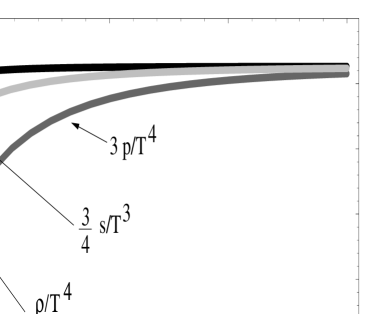
Figure 2: Scaled energy density $\rho$ (black), pressure $p$ (dark gray), and entropy density $s$ (light gray) in the deconfining phase of SU(2) Yang-Mills thermodynamics.

In Fig. 2 we report the (scaled) energy density $\rho$, pressure $p$, and entropy density $s$ as functions of temperature. A detailed comparison of these results with those obtained on the lattice (for both differential and integral method and for the SU(3) case) is carried out in [12]. While there is good agreement for the entropy density $s$ (for which the ground state is not relevant) the pressure $p$ becomes negative close to the phase boundary in virtue of the negative contribution of the ground state. While this is in qualitative agreement with the result of the differential method, it is not with that of the integral method. This fact, as emphaiszed in the Introduction, represents a motivation to perform the present work where lattice results safely above the phase boundary, such as the behavior of $\theta_{\mu\mu}$ at high $T$, are compared with the effective approach under study.

4 The SU(3) case

In the SU(3) case the behavior of $\theta_{\mu\mu}$ is qualitatively similar to the SU(2) case. We only report on some relevant formulas and briefly discuss their consequences. The modulus of the scalar field $\phi$ is exactly the same. As shown in [12] out of the eight coarse-grained gauge modes four acquire a mass $m_{1}=e\left|\phi\right|$ (contributing to $\rho$ and $p$ by $\rho_{1}$ and $p_{1}$), two a mass $m_{2}=2e\left|\phi\right|$ ($\rho_{2}$ and $p_{2}$), and two stay massless ($\rho_{3}$ and $p_{3}$). Explicitly, we have ($a=m_{1}/T$):

$$\overline{\rho}_{3} = 4\,\frac{\pi^{2}}{30}\,,\ \text{ }\overline{\rho}_{1}=\frac{6}{\pi^{2}}\int_{0}^{\infty}dx\,\frac{x^{2}\sqrt{x^{2}+a^{2}}}{e^{\sqrt{x^{2}+a^{2}}}-1}\,,$$ (20)

$$\overline{\rho}_{2} = \frac{3}{\pi^{2}}\int_{0}^{\infty}dx\,\frac{x^{2}\sqrt{x^{2}+(2a)^{2}}}{e^{\sqrt{x^{2}+(2a)^{2}}}-1}\,,\ \text{ }\overline{\rho}_{gs}=\frac{2(2\pi)^{4}}{\lambda^{3}}\,,$$ (21)

$$\overline{p}_{3} = 4\,\frac{\pi^{2}}{90}\,,\ \text{ }\overline{p}_{1}=-\frac{6}{\pi^{2}}\int_{0}^{\infty}dx\,x^{2}\ln\left(1-e^{-\sqrt{x^{2}+a^{2}}}\right)\,,\text{ }$$ (22)

$$\overline{p}_{2} = -\frac{3}{\pi^{2}}\int_{0}^{\infty}dx\,x^{2}\ln\left(1-e^{-\sqrt{x^{2}+(2a)^{2}}}\right)\,,\ \text{ }\overline{p}_{gs}=-\text{ }\overline{\rho}_{gs}\,.$$ (23)

Eq. (9) assumes the following form:

$$1=-\frac{12\lambda^{3}}{(2\pi)^{6}}\left(\lambda\frac{da}{d\lambda}+a\right)\left(aD(a)+2aD(2a)\right)\,.$$ (24)

The asymptotic solution to Eq. (24) reads $a(\lambda)=\frac{8}{\sqrt{3}}\pi^{2}\lambda^{-3/2}$, and the effective coupling reaches a plateau value of $e=\frac{4}{\sqrt{3}}\pi.$ The value for $\lambda_{c}$ is $\lambda_{c}=9.475$ [12] where the coupling and all masses diverge. The function $h(\lambda)$, defined in (14), has an asymptotic value of $3/2$ like in the SU(2) case. Thus the asymptotically linear behavior $\theta_{\mu\mu}=\rho-3p=24\pi\Lambda^{3}T$ holds. Relating $\Lambda$ to the critical temperature $T_{c}$ as in Eq. (18), we take into account the SU(3)-value $\lambda_{c}=9.475$. This yields:

$$\theta_{\mu\mu}=\rho-3p=\frac{192\pi^{4}}{\lambda_{c}^{3}}T_{c}^{3}T\simeq 21.9\,T_{c}^{3}T\,.$$ (25)

As in Ref. [1] we set $T_{c}=0.264$ GeV and thus find $\theta_{\mu\mu}\simeq 0.4\,T\,\mbox{GeV}^{3}$ for $T\gg T_{c}$. In [1] a somewhat smaller slope of $\simeq 0.2$ GeV³ is extracted. In [3] a slope of $0.63$ GeV³ was estimated.

5 Conclusions

In this paper we studied the high-temperature behavior of the trace of the stress-energy tensor $\theta_{\mu\mu}=\rho-3p.$ This quantity measures the breaking of scale invariance and vanishes for a relativist gas of free gluons: recent lattice works [1, 2] show a linear rise for high $T$ (see however also [6], where the rise is quadratic). This means that strong interactions still play a decisive role even in the high temperature domain.

Theoretical studies should therefore be concerned with the predicted behavior of $\theta_{\mu\mu}$ at high temperatures. We have shown that the linear growth of $\theta_{\mu\mu}$ for high $T$ is an analytic prediction of the approach to Yang-Mills thermodynamics [12], which involves a thermal ground state emerging as an average over instantons at finite $T$. That is, even in the high-$T$ limit the dynamic of these field configurations is important and can be detected by lattice simulations. In both cases, SU(2) and SU(3), we evaluated the slope of $\theta_{\mu\mu}$ and the results $\theta_{\mu\mu}\simeq 7\,T_{c}^{3}T\,$and $\theta_{\mu\mu}\simeq 21.9\,T_{c}^{3}T\,,\$where $T_{c}$ is the deconfining temperature, are found for high $T$, respectively. We compared to the lattice results of Miller [1, 2] and to the theoretical work of Zwanziger [3] finding good agreement. In the latter a momentum-dependent, universal modification of the dispersion relation for propagating, fundamental gluon fields, motivated by the reduction of the physical state space a la Gribov, is introduced. Our approach and [3] share the property of a nonpertrubative gluon mass leading to the linear growth of $\theta_{\mu\mu}$. However, while in our case the mass is a temperature-dependent coarse grained quantity and the ground state itsself contributes to $\theta_{\mu\mu},$ this is not the case in [3]. A more detailed comparison would be surely interesting but goes beyond the scope of the present work.

We believe that future studies on the high $T$ behavior of $\theta_{\mu\mu}$ are therefore very important, both numerically and analytically, in order to confirm the linear growth and to relate it to nonperturbative aspects of Yang-Mills theories.

References

- [1] D. E. Miller, arXiv:hep-ph/0608234.
- [2] D. E. Miller, Acta Phys. Polon. B 28 (1997) 2937.
- [3] D. Zwanziger, Phys. Rev. Lett. 94 (2005) 182301.
- [4] G. Boyd and D. E. Miller, arXiv:hep-ph/9608482.
- [5] J. Engels, F. Karsch and K. Redlich, Nucl. Phys. B 435 (1995) 295 [arXiv:hep-lat/9408009]. G. Boyd, J. Engels, F. Karsch, E. Laermann, C. Legeland, M. Lutgemeier and B. Petersson, Nucl. Phys. B 469 (1996) 419 [arXiv:hep-lat/9602007].
- [6] R. D. Pisarski, arXiv:hep-ph/0612191.
- [7] R. A. Schneider and W. Weise, Phys. Rev. C 64 (2001) 055201.
- [8] D. H. Rischke, J. Schaffner, M. I. Gorenstein, A. Schaefer, H. Stoecker and W. Greiner, Z. Phys. C 56 (1992) 325.
- [9] P. Levai and U. W. Heinz, Phys. Rev. C 57 (1998) 1879.
-
[10]
D. J. Gross and Frank Wilczek, Phys. Rev. D 8,
3633 (1973).
D. J. Gross and Frank Wilczek, Phys. Rev. Lett. 30, 1343 (1973).
H. David Politzer, Phys. Rev. Lett. 30, 1346 (1973).
H. David Politzer, Phys. Rept. 14, 129 (1974). - [11] M. Laine and Y. Schroder, Phys. Rev. D 73 (2006) 085009 [arXiv:hep-ph/0603048]. K. Kajantie, M. Laine, K. Rummukainen and Y. Schroder, Phys. Rev. D 67 (2003) 105008 [arXiv:hep-ph/0211321].
-
[12]
R. Hofmann,
Int. J. Mod. Phys. A20 (2005) 4123, Erratum-ibid. A 21
(2006) 6515.
R. Hofmann, Mod. Phys. Lett. A21, 999 (2006), Erratum-ibid. A 21, 3049 (2006). - [13] F. R. Brown, N. H. Christ, Y. F. Deng, M. S. Gao and T. J. Woch, Phys. Rev. Lett. 61 (1988) 2058.
- [14] J. Engels, J. Fingberg, F. Karsch, D. Miller and M. Weber, Phys. Lett. B 252 (1990) 625.
- [15] A. D. Linde, Phys. Lett. B 96 (1980) 289.
- [16] F. Giacosa and R. Hofmann, arXiv:hep-th/0609172.
- [17] U. Herbst and R. Hofmann, arXiv:hep-th/0411214.
- [18] R. Hofmann, arXiv:hep-th/0609033.
- [19] D. H. Rischke, Prog. Part. Nucl. Phys. 52 (2004) 197.
- [20] W. Nahm, Lect. Notes in Physics. 201, eds. G. Denaro, e.a. (1984) p. 189.
-
[21]
K.-M. Lee and C.-H. Lu, Phys. Rev. D 58, 025011 (1998).
T. C. Kraan and P. van Baal, Nucl. Phys. B 533, 627 (1998).
T. C. Kraan and P. van Baal, Phys. Lett. B 435, 389 (1998). - [22] M. Schwarz, R. Hofmann and F. Giacosa, arXiv:hep-th/0603078 (in press Int. J. Mod. Phys. A).
- [23] L. Dolan and R. Jackiw, Phys. Rev. D 9, 3320 (1974).
- [24] K. Langfeld, E. M. Ilgenfritz, H. Reinhardt and G. Shin, Nucl. Phys. Proc. Suppl. 106 (2002) 501 [arXiv:hep-lat/0110024].