hep-th/0703126

March, 2007

Effective action of $\beta$-deformed ${\cal N}=4$ SYM theory:
Farewell to two-loop BPS diagrams

Sergei M. Kuzenko and Ian N. McArthur

School of Physics M013, The University of Western Australia
35 Stirling Highway, Crawley W.A. 6009, Australia  

Within the background field approach, all two-loop sunset vacuum diagrams, which occur in the Coulomb branch of ${\cal N}=2$ superconformal theories (including ${\cal N}=4$ SYM), obey the BPS condition $m_{3}=m_{1}+m_{2}$, where the masses are generated by the scalars belonging to a background ${\cal N}=2$ vector multiplet. These diagrams can be evaluated exactly, and prove to be homogeneous quadratic functions of the one-loop tadpoles $J(m_{1}^{2})$, $J(m_{2}^{2})$ and $J(m_{3}^{2})$, with the coefficients being rational functions of the squared masses. We demonstrate that, if one switches on the $\beta$-deformation of the ${\cal N}=4$ SYM theory, the BPS condition no longer holds, and then generic two-loop sunset vacuum diagrams with three non-vanishing masses prove to be characterized by the following property: $2(m_{1}^{2}m_{2}^{2}+m_{1}^{2}m_{3}^{2}+m_{2}^{2}m_{3}^{2})>m_{1}^{4}+m_{2}^{4}+m_{3}^{4}$. In the literature, there exist several techniques to compute such diagrams. For the $\beta$-deformed ${\cal N}=4$ SYM theory, we carry out explicit two-loop calculations of the Kähler potential and $F^{4}$ term. Our considerations are restricted to the case of $\beta$ real.

 

1 Introduction

In the family of finite ${\cal N}=1$ supersymmetric theories (see [2, 3] for an incomplete list of references), the exactly marginal $\beta$-deformation [4] of the ${\cal N}=4$ $SU(N)$ SYM theory has recently attracted some renewed attention, for it has been shown to possess a supergravity dual description [5]. In particular, in addition to stringy and non-perturbative aspects, various field-theoretic properties of the $\beta$-deformed SYM have been studied at the perturbative level, see [6, 7, 8, 9, 10, 11, 12, 13, 14] and references therein. Naturally, it is of special interest to understand what features of the ${\cal N}=4$ SYM theory survive the deformation, as well as to determine new dynamical properties generated by the deformation. Of course, there are many non-trivial differences between the deformed and undeformed theories, and here we mention only a few of them.

Unlike the ${\cal N}=4$ SYM theory, the finiteness condition in the deformed theory receives “quantum corrections” at different loop orders [6, 7, 8, 3]. This condition is known exactly only for the real deformation in the large $N$ limit [9]. It is an exciting open problem to determine the exact condition for superconformal invariance at finite $N$. We should point out that very interesting and conflicting results have appeared regarding the fate of superconformal invariance for the complex deformation [12, 13]. Since a more detailed analysis of this issue is desirable, our consideration in this paper is restricted to the case of real $\beta$.

As is well-known, in the Coulomb branch of general ${\cal N}=2$ SYM theories, there are no quantum corrections to the effective Kähler potential beyond one loop, and no one-loop quantum corrections in the ${\cal N}=2$ superconformal models. In the $\beta$-deformed ${\cal N}=4$ SYM theory, however, one can expect the generation of a non-trivial superconformally invariant Kähler potential at two and higher loops. Similar holomorphic quantum corrections in the gauge sector are already generated at one loop [10, 15]:

$$\frac{1}{16\pi^{2}}\,\int{\rm d}^{2}\theta\sum_{i<j}\Big{(}W^{i}-W^{j}\Big{)}^{2}\,\ln\Bigg{[}\frac{g^{2}(\phi^{i}-\phi^{j})^{2}}{h^{2}\,(q\,\phi^{i}-q^{-1}\,\phi^{j})(q^{-1}\,\phi^{i}-q\,\phi^{j})}\Bigg{]}~{}.$$ (1.1)

Here the ${\cal N}=1$ chiral scalars $\Phi={\rm diag}\,(\phi^{1},\dots,\phi^{N})$ and gauge-invariant field strengths ${\cal W}_{\alpha}={\rm diag}\,(W^{1}_{\alpha},\dots,W^{N}_{\alpha})$ constitute a ${\cal N}=2$ vector multiplet in the Cartan subalgebra of $SU(N)$, such that $\sum_{i=1}^{N}\phi^{i}=\sum_{i=1}^{N}W^{i}_{\alpha}=0$. The above quantum correction disappears if the deformation parameters $q=\exp({\rm i}\pi\beta)$ and $h$ take the values $q=1$ and $h=g$ corresponding to the ${\cal N}=4$ SYM theory, with $g$ the Yang-Mills coupling constant.

The present paper, which is a continuation of [10], is aimed at uncovering another interesting dynamical property of the $\beta$-deformed theory that distinguishes it from the ${\cal N}=4$ SYM theory, and more generally from the ${\cal N}=2$ superconformal models. It concerns the structure of two-loop sunset diagrams with different masses, which have been studied by many groups including [16, 17, 18, 19, 20]. We begin with a few general comments about such Feynman diagrams.

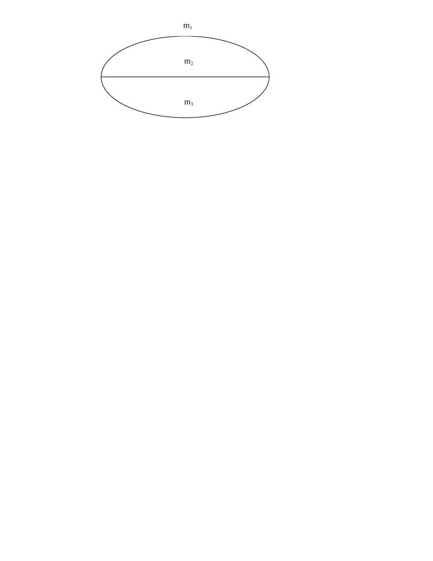
Figure 1: Two-loop sunset diagram

When computing low energy effective actions within the background field formalism, one has to deal with two-loop sunset vacuum integrals of the general form

$$I(\nu_{1},\nu_{2},\nu_{3};m_{1}^{2},m_{2}^{2},m_{3}^{2})=\frac{(\mu^{2})^{4-d}}{(2\pi)^{2d}}\int\frac{{\rm d}^{d}k\,{\rm d}^{d}q}{(k^{2}+m_{1}^{2})^{\nu_{1}}(q^{2}+m_{2}^{2})^{\nu_{2}}((k+q)^{2}+m_{3}^{2})^{\nu_{3}}}~{},~{}~{}~{}$$ (1.2)

with $\nu_{1}$, $\nu_{2}$ and $\nu_{3}$ non-negative integers, see Fig. 1. Davydychev and Tausk [18] derived recurrence relations that allow one to express $I(\nu_{1},\nu_{2},\nu_{3};m_{1}^{2},m_{2}^{2},m_{3}^{2})$ in terms of the master integral $I(1,1,1;m_{1}^{2},m_{2}^{2},m_{3}^{2})$ and a product of one-loop tadpoles

$$J(m^{2})=\frac{(\mu^{2})^{2-d/2}}{(2\pi)^{d}}\int\frac{{\rm d}^{d}k}{k^{2}+m^{2}}=\frac{(\mu^{2}/m^{2})^{2-d/2}}{(4\pi)^{d/2}}\,m^{2}\,\Gamma(1-d/2)~{}.$$ (1.3)

The recurrence relations obtained in [18] are:

$${\mathbb{I}}(\nu_{1}+1,\nu_{2},\nu_{3})=-\,\frac{1}{\nu_{1}m_{1}^{2}\Delta(m_{1}^{2},m_{2}^{2},m_{3}^{2})}\Big{\{}{\mathbb{I}}(\nu_{1},\nu_{2},\nu_{3})\Big{[}\nu_{2}(m_{1}^{2}-m_{3}^{2})(m_{1}^{2}-m_{2}^{2}+m_{3}^{2})$$

$$\quad+\nu_{3}(m_{1}^{2}-m_{2}^{2})(m_{1}^{2}+m_{2}^{2}-m_{3}^{2})+d\,m_{1}^{2}(m_{1}^{2}-m_{2}^{2}+m_{3}^{2})-\nu_{1}\Delta(m_{1}^{2},m_{2}^{2},m_{3}^{2})\Big{]}$$

$$\quad+\nu_{2}m_{2}^{2}(m_{1}^{2}-m_{2}^{2}+m_{3}^{2})\Big{[}{\mathbb{I}}(\nu_{1},\nu_{2}+1,\nu_{3}-1)-{\mathbb{I}}(\nu_{1}-1,\nu_{2}+1,\nu_{3})\Big{]}$$

$$\quad+\nu_{3}m_{3}^{2}(m_{1}^{2}+m_{2}^{2}-m_{3}^{2})\Big{[}{\mathbb{I}}(\nu_{1},\nu_{2}-1,\nu_{3}+1)-{\mathbb{I}}(\nu_{1}-1,\nu_{2},\nu_{3}+1)\Big{]}\Big{\}}~{},$$ (1.4)

where we have used the condensed notation ${\mathbb{I}}(\nu_{1},\nu_{2},\nu_{3})\equiv I(\nu_{1},\nu_{2},\nu_{3};m_{1}^{2},m_{2}^{2},m_{3}^{2})$, and

$$\Delta(m_{1}^{2},m_{2}^{2},m_{3}^{2})=2(m_{1}^{2}m_{2}^{2}+m_{1}^{2}m_{3}^{2}+m_{2}^{2}m_{3}^{2})-(m_{1}^{4}+m_{2}^{4}+m_{3}^{4})~{}.$$ (1.5)

The master integral $I(1,1,1;m_{1}^{2},m_{2}^{2},m_{3}^{2})$ can be evaluated using the techniques developed, e.g., in [17, 18, 20].

On the Coulomb branch of ${\cal N}=2$ superconformal theories, we have $U(1)$ charge conservation at each vertex of the supergraphs. In particular, for the two-loop sunset diagrams we get

$$e_{1}+e_{2}+e_{3}=0~{}.$$ (1.6)

Because of the BPS condition $m_{i}=Z|e_{i}|$, the requirement of charge conservation implies

$$m_{1}=m_{2}+m_{3}~{},\quad{\rm or}\quad~{}m_{2}=m_{1}+m_{3}~{},\quad{\rm or}\quad~{}m_{3}=m_{1}+m_{2}~{}.$$ (1.7)

This leads to the condition

$$\Delta(m_{1}^{2},m_{2}^{2},m_{3}^{2})=0~{}$$ (1.8)

in arbitrary ${\cal N}=2$ superconformal theories, due to the factorization property [21, 20]

$$\frac{\Delta(m_{1}^{2},m_{2}^{2},m_{3}^{2})}{m_{1}+m_{2}+m_{3}}=(m_{1}+m_{2}-m_{3})(m_{1}-m_{2}+m_{3})(-m_{1}+m_{2}+m_{3})~{}.$$ (1.9)

As a result, the recurrence relations (1.4) cannot be applied. Also, because of (1.8), we cannot generate integrals (1.2) with arbitrary $\nu_{i}$ from $I(1,1,1;m_{1}^{2},m_{2}^{2},m_{3}^{2})$ by differentiation with respect to $m_{i}^{2}$. In other words, special consideration is required in order to compute momentum integrals (1.2) under the BPS condition (1.8).

Actually, recurrence relations for the case (1.8) have been found by Tarasov [21]. They imply that all BPS integrals (1.2) are given in terms of elementary functions, unlike the generic case $\Delta(m_{1}^{2},m_{2}^{2},m_{3}^{2})\neq 0$, where integral representations for $I(1,1,1;m_{1}^{2},m_{2}^{2},m_{3}^{2})$ involve transcendental functions [17, 18, 20]. More precisely, the BPS integrals are homogeneous quadratic functions of the one-loop tadpoles $J(m_{1}^{2})$, $J(m_{2}^{2})$ and $J(m_{3}^{2})$, with the coefficients being rational functions of the squared masses. In the present paper, we will re-derive this result using several different approaches.

If one switches from the ${\cal N}=4$ SYM theory to its $\beta$-deformation, it turns out that the BPS condition (1.8) no longer holds. As is shown below, with $\beta$ real, one typically has $\Delta(m_{1}^{2},m_{2}^{2},m_{3}^{2})>0$ if all masses are non-vanishing. Two-loop calculations of the effective action become much more involved, as compared with the ${\cal N}=4$ case, and one has to use the full power of the techniques developed in [17, 18, 20].

This paper is organized as follows. In section 2 we give a detailed study of integrals (1.2) under the BPS condition (1.8). Section 3 is devoted to various aspects of the background field quantization of the $\beta$-deformed ${\cal N}=4$ SYM theory, including the specification of the background superfields chosen. In section 4 the two-loop contributions to the effective action are decomposed into a set of terms involving only $U(1)$ Green’s functions. Exact covariant superpropagators are given in section 5. The two-loop quantum corrections are evaluated in section 6. Two technical appendices are included at the end of the paper. Appendix A reviews and elaborates on the approach developed in [17]. Appendix B contains the $SU(N)$ conventions adopted in this paper.

2 Two-loop BPS integrals

Consider a vacuum two-loop integral $I(\nu_{1},\nu_{2},\nu_{3};x,y,z)$ as in (1.2), with $\nu_{1},\nu_{2}$ and $\nu_{3}$ non-negative integers, and $(x,y,z)=(m_{1}^{2},m_{2}^{2},m_{3}^{2})$. Under the BPS condition $\Delta(x,y,z)=0$, this integral turns out to be a homogeneous quadratic function of $J(x)$, $J(y)$ and $J(z)$, with the coefficients being rational functions of $x$, $y$ and $z$. The simplest way to establish this result is by making use of a differential equation for the completely symmetric master integral $I(x,y,z)=I(1,1,1;x,y,z)$, defined in eq. (A.1), that was presented in [20].

Using eq. (A.3) and two more equations that follow from (A.3) by applying cyclic permutations of $x$, $y$ and $z$, one can deduce a differential equation involving a single partial derivative of $I$, say with respect to $z$ [20]. It reads

$$\Delta(x,y,z)\,\frac{\partial}{\partial z}I(x,y,z)=(d-3)(x+y-z)I(x,y,z)$$

$$\qquad+\frac{2-d}{2}\Big{\{}\frac{-x+y+z}{z}J(x)J(z)+\frac{x-y+z}{z}J(y)J(z)-2J(x)J(y)\Big{\}}~{},$$ (2.1)

with $\Delta(x,y,z)$ defined in (1.5). Implementing cyclic permutations of $x$, $y$ and $z$, one generates two more equivalent equations.

Now, let us apply an operator

$$\frac{\partial^{\nu_{1}+\nu_{2}+\nu_{3}}}{\partial x^{\nu_{1}}\partial y^{\nu_{2}}\partial z^{\nu_{3}}}$$

to both sides of eq. (2.1), and in the end impose the BPS condition $\Delta(x,y,z)=0$. The latter implies that the term of highest order in derivatives of $I$ drops out.

Using the condensed notation ${\mathbb{I}}(\nu_{1},\nu_{2},\nu_{3})\equiv I(\nu_{1},\nu_{2},\nu_{3};x,y,z)$, on the two-dimensional surface $\Delta(x,y,z)=0$ we obtain the following algebraic equations:

$$\nu_{1}\frac{\partial\Delta}{\partial x}{\mathbb{I}}(\nu_{1},1+\nu_{2},2+\nu_{3})\,(\nu_{1}-1)!\nu_{2}!(\nu_{3}+1)!$$

$$\quad+\nu_{2}\frac{\partial\Delta}{\partial y}{\mathbb{I}}(1+\nu_{1},\nu_{2},2+\nu_{3})\,\nu_{1}!(\nu_{2}-1)!(\nu_{3}+1)!$$

$$\quad+\frac{1}{2}(2\nu_{3}-d+3)\frac{\partial\Delta}{\partial z}{\mathbb{I}}(1+\nu_{1},1+\nu_{2},1+\nu_{3})\,\nu_{1}!\nu_{2}!\nu_{3}!$$

$$\quad+\nu_{3}(\nu_{3}-d+2){\mathbb{I}}(1+\nu_{1},1+\nu_{2},\nu_{3})\,\nu_{1}!\nu_{2}!(\nu_{3}-1)!$$

$$\quad+\nu_{1}(\nu_{1}-1){\mathbb{I}}(\nu_{1}-1,1+\nu_{2},2+\nu_{3})\,(\nu_{1}-2)!\nu_{2}!(\nu_{3}+1)!$$

$$\quad+\nu_{2}(\nu_{2}-1){\mathbb{I}}(1+\nu_{1},\nu_{2}-1,2+\nu_{3})\,\nu_{1}!(\nu_{2}-2)!(\nu_{3}+1)!$$

$$\quad-2\nu_{1}\nu_{2}{\mathbb{I}}(\nu_{1},\nu_{2},2+\nu_{3})\,(\nu_{1}-1)!(\nu_{2}-1)!(\nu_{3}+1)!$$

$$\quad+(d-3-2\nu_{3})\Big{\{}\nu_{1}{\mathbb{I}}(\nu_{1},1+\nu_{2},1+\nu_{3})\,(\nu_{1}-1)!\nu_{2}!$$

$$\qquad\qquad\qquad\qquad+\nu_{2}{\mathbb{I}}(1+\nu_{1},\nu_{2},1+\nu_{3})\,\nu_{1}!(\nu_{2}-1)!\Big{\}}\nu_{3}!$$

$$=(-1)^{\nu_{1}+\nu_{2}+\nu_{3}}\frac{2-d}{2}\frac{\partial^{\nu_{1}+\nu_{2}+\nu_{3}}}{\partial x^{\nu_{1}}\partial y^{\nu_{2}}\partial z^{\nu_{3}}}\Big{\{}\frac{-x+y+z}{z}J(x)J(z)+\frac{x-y+z}{z}J(y)J(z)$$

$$\qquad\qquad\qquad\qquad\qquad\qquad\qquad-2J(x)J(y)\Big{\}}\Big{|}_{\Delta(x,y,z)=0}~{}.$$ (2.2)

Eq. (2.2) constitutes recurrence relations allowing one to compute, for even $d$, arbitrary two-loop integrals $I(\nu_{1},\nu_{2},\nu_{3};x,y,z)$, with $\nu_{1},\nu_{2},\nu_{3}=1,2,\dots$, under the BPS condition $\Delta(x,y,z)=0$ and the assumption that all three masses are non-vanishing. Choosing $\nu_{1}=\nu_{2}=\nu_{3}=0$ in (2.2) gives [17, 20, 39]

$$I_{\rm BPS}(x,y,z)=\frac{d-2}{2(d-3)}\,\frac{1}{\partial_{z}\Delta}\Big{\{}\frac{\partial_{x}\Delta}{z}J(x)J(z)+\frac{\partial_{y}\Delta}{z}J(y)J(z)-4J(x)J(y)\Big{\}}$$ (2.3)

$$= -\frac{d-2}{4(d-3)}\Big{\{}\frac{x-y+z}{xz}J(x)J(z)+\frac{-x+y+z}{yz}J(y)J(z)+\frac{x+y-z}{xy}J(x)J(y)\Big{\}}~{}.~{}~{}~{}~{}~{}~{}~{}~{}$$

Here we have used the BPS restrictions of the identities

$$\frac{1}{4}\partial_{x}\Delta\,\partial_{y}\Delta=\Delta-z\partial_{z}\Delta~{},\quad\frac{1}{4}\partial_{x}\Delta\,\partial_{z}\Delta=\Delta-y\partial_{y}\Delta~{},\quad\frac{1}{4}\partial_{y}\Delta\,\partial_{z}\Delta=\Delta-x\partial_{x}\Delta~{}~{}~{}~{}$$ (2.4)

and

$$\frac{1}{4}\big{(}\partial_{x}\Delta\big{)}^{2}+\Delta=4yz~{},\quad\frac{1}{4}\big{(}\partial_{y}\Delta\big{)}^{2}+\Delta=4xz~{},\quad\frac{1}{4}\big{(}\partial_{z}\Delta\big{)}^{2}+\Delta=4xy~{},$$ (2.5)

to bring $I(x,y,z)$ to a manifestly symmetric form with respect to $x,$ $y$ and $z$. As is seen from these identities, the combitations $\partial_{x}\Delta$, $\partial_{y}\Delta$ and $\partial_{z}\Delta$ are non-zero at $\Delta=0$. In addition, two of them are positive and the third negative. Indeed, without loss of generality, we can choose $x=m_{1}^{2}$, $y=m_{2}^{2}$ and $z=(m_{1}+m_{2})^{2}$, so that for the combinations $\partial_{x}\Delta=2(-x+y+z)$, $\partial_{y}\Delta=2(x-y+z)$ and $\partial_{z}\Delta=2(x+y-z)$ we get

$$\partial_{x}\Delta=4m_{2}(m_{1}+m_{2})~{},\quad\partial_{y}\Delta=4m_{1}(m_{1}+m_{2})~{},\quad\partial_{z}\Delta=-4m_{1}m_{2}~{}.$$ (2.6)

As a less trivial example, choosing $\nu_{1}=\nu_{2}=0$ and $\nu_{3}=1$ in (2.2) gives

$$I_{\rm BPS}(1,1,2;x,y,z) = \frac{d-2}{4(5-d)}\frac{1}{xyz^{2}}\Big{[}y\Big{\{}z-\frac{1}{2}(d-4)(x-y+z)\Big{\}}J(x)J(z)$$ (2.7)

$$+x\Big{\{}z-\frac{1}{2}(d-4)(-x+y+z)\Big{\}}J(y)J(z)-z^{2}J(x)J(y)\Big{]}~{}.~{}~{}~{}$$

More generally, choosing $\nu_{1}=\nu_{2}=0$ and $\nu_{3}>0$ in (2.2) gives the recurrence relation:

$$I_{\rm BPS}(1,1,1+\nu;x,y,z)=\frac{1}{(2\nu+3-d)(x+y-z)}\Bigg{[}(d-2-\nu)I(1,1,\nu;x,y,z)$$

$$\qquad\qquad+\frac{(-1)^{\nu}}{\nu!\,2^{\nu+1}}(d-2)(d-4)\dots(d-2\nu)\,\frac{J(z)}{z^{\nu+1}}$$

$$\qquad\qquad\times\Big{\{}(d-2-2\nu)(x-y)\big{(}J(x)-J(y)\big{)}-(d-2)z\big{(}J(x)+J(y)\big{)}\Big{\}}\Bigg{]}~{}.~{}~{}~{}~{}$$ (2.8)

The recurrence relations (2.2) look somewhat messy, although their derivation is completely trivial. More elegant recurrence relations, albeit equivalent to eq. (2.2), were derived in [21]. In both cases, the recurrence relations clearly demonstrate that the BPS integrals are homogeneous quadratic functions of the one-loop tadpoles $J(x)$, $J(y)$ and $J(z)$, with the coefficients being rational functions of the squared masses.

In practical terms, it may be simpler to compute the two-loop BPS integrals by first differentiating the expression in eq. (A.34) for the master integral with respect to $x$, $y$ and $z$, and then implementing the limit $\Delta\to 0$. This requires certain care, since the limit $\Delta\to 0$ is actually singular (one should also make use of the fact that, among the combinations $\partial_{x}\Delta$, $\partial_{y}\Delta$ and $\partial_{z}\Delta$, two are positive, and the third negative, as eq. (2.6) explicitly shows). As an example, let us evaluate $I(1,1,2;x,y,z)|_{\Delta=0}$ using the functional representation (A.34). Differentiating the right-hand side of (A.34) with respect to $z$ and then setting $\Delta=0$ gives

$$I_{\rm BPS}(1,1,2;x,y,z)=\frac{\Gamma^{\prime}}{2(1+2\epsilon)}\Bigg{\{}(xy)^{-\epsilon} - (xz)^{-\epsilon}\Big{[}1+2\epsilon+2\epsilon\,\frac{\partial_{z}\Delta}{\partial_{y}\Delta}\Big{]}$$ (2.9)

$$- (yz)^{-\epsilon}\Big{[}1+2\epsilon+2\epsilon\,\frac{\partial_{z}\Delta}{\partial_{x}\Delta}\Big{]}\Bigg{\}}~{},$$

with $\Gamma^{\prime}$ given in eq. (A.8). This can be seen to agree with the representation (2.7) if one makes use of (2.6).

The powerful techniques developed in [17] and [18] to compute the two-loop master integral $I(x,y,z)$, eq. (A.1), are quite involved. Remarkably, the first-order inhomogeneous ODE (2.1) and the value of $I(x,y,z)$ at $\Delta=0$, eq. (2.3), comprise all the ingredients one needs to compute $I(x,y,z)$ by elementary means [20], in the case with three non-vanishing masses. Let us consider, for definiteness, the domain $\Delta(x,y,z)>0$. Eq. (2.1) is integrated as follows:

$$I(x,y,z) = -\Delta^{(d-3)/2}(x,y,z)\,\Big{\{}\int\limits_{z_{0}}^{z}{\rm d}t\,\frac{\Psi(x,y,t)}{\Delta^{(d-1)/2}(x,y,t)}+\frac{I(x,y,z_{0})}{\Delta^{(d-3)/2}(x,y,z_{0})}\Big{\}}~{},$$ (2.10)

$$\Psi(x,y,z) = \frac{1}{2}\Big{\{}\partial_{x}\Delta\,J(x)J^{\prime}(z)+\partial_{y}\Delta\,J(y)J^{\prime}(z)-2(d-2)J(x)J(y)\Big{\}}~{},$$

for some $z_{0}$ such that $\Delta(x,y,z_{0})>0$. Since the right-hand side of (2.10) does not depend on $z_{0}$, we can consider the limit $z_{0}\to z_{\rm BPS}=(m_{1}+m_{2})^{2}$, with the latter point such that $\Delta(x,y,z_{\rm BPS})=0$ and $I(x,y,z_{\rm BPS})=I_{\rm BPS}(x,y,z_{\rm BPS})$. In this limit, however, the integral in (2.10) becomes singular at the lower limit. To get rid of singularities, we can first integrate by parts in (2.10) by making use of the third identity in (2.5). More precisely, using the identity

$$\frac{1}{\Delta^{n+1}}=\frac{1}{4xy}\,\Big{\{}\frac{1}{\Delta^{n}}-\frac{\partial_{t}\Delta}{4n}\,\partial_{t}\Big{(}\frac{1}{\Delta^{n}}\Big{)}\Big{\}}~{},\qquad\Delta=\Delta(x,y,t)$$ (2.11)

on the right of (2.10) in order to integrate by parts, and then implementing the limit $z_{0}\to z_{\rm BPS}$, we obtain

$$I(x,y,z) = -\frac{\Delta^{(d-3)/2}(x,y,z)}{4(d-3)xy}\,\int\limits_{z_{\rm BPS}}^{z}{\rm d}t\,\frac{\Psi_{1}(x,y,t)}{\Delta^{(d-3)/2}(x,y,t)}+\frac{\Psi(x,y,z)\,\partial_{z}\Delta(x,y,z)}{8(d-3)xy}~{},~{}~{}~{}~{}~{}$$ (2.12)

$$\Psi_{1}(x,y,z) = (d-4)\Psi+\frac{1}{2}\partial_{z}\Delta\,\partial_{z}\Psi~{}.$$

The first term on the right of (2.12) can again be integrated by parts, using the identity (2.11), and so on. This can be seen to generate a representation for $I(x,y,z)$ as a series in powers of $\Delta$. In particular, for any positive integer $k$ we have

$$I(x,y,z) = -\frac{\Delta^{(d-3)/2}(x,y,z)}{(d-3)(d-5)\cdots(d-3-2k)}\Big{(}\frac{1}{4xy}\Big{)}^{k+1}\,\int\limits_{z_{\rm BPS}}^{z}{\rm d}t\,\frac{\Psi_{k+1}(x,y,t)}{\Delta^{(d-3-2k)/2}(x,y,t)}$$ (2.13)

$$+\frac{\partial_{z}\Delta(x,y,z)}{8xy}\sum_{p=0}^{k}\Big{(}\frac{\Delta(x,y,z)}{4xy}\Big{)}^{p}\frac{\Psi_{p}(x,y,z)}{(d-3)(d-5)\cdots(d-3-2p)}~{},$$

with

$$\Psi_{k+1}=(d-4-2k)\Psi_{k}+\frac{1}{2}\partial_{z}\Delta\,\partial_{z}\Psi_{k}~{},\qquad\Psi_{0}=\Psi~{}.$$ (2.14)

This representation is useful, e.g., for an alternative evaluation of the BPS integrals.

To conclude this section, we note that an alternative solution to equation (2.1) was given in [20] in the context of the epsilon-expansion.

3 The $\beta$-deformed ${\cal N}$ = 4 SYM theory

The $\beta$-deformed ${\cal N}=4$ $SU(N)$ SYM theory is described by the action

$$S = \int{\rm d}^{8}z\,{\rm tr}\,(\Phi_{i}^{\dagger}\,\Phi_{i})+\frac{1}{g^{2}}\int{\rm d}^{6}z\,{\rm tr}({\cal W}^{\alpha}{\cal W}_{\alpha})$$ (3.1)

$$+\Big{\{}h\int{\rm d}^{6}z\,{\rm tr}(q\,\Phi_{1}\Phi_{2}\Phi_{3}-q^{-1}\,\Phi_{1}\Phi_{3}\Phi_{2})~{}+~{}{\rm c.c.}\Big{\}}~{},\ \ \ \ \ q\equiv{\rm e}^{{\rm i}\pi\beta}\ ,$$

where $q$ is the deformation parameter, $g$ is the gauge coupling constant, and $h$ is related to $g$ and $q$ by the condition of quantum conformal invariance. The latter is not yet known exactly, since it is expected to receive quantum corrections at arbitrary loop orders, and the higher loop corrections are hard to evaluate in closed form. To two-loop order, the condition of quantum conformal invariance for real $\beta$ is as follows [6, 7, 3] (see also [22]):

$$|h|^{2}\,\Big{(}1-{1\over N^{2}}\,\Big{|}q-{1\over q}\Big{|}^{2}\Big{)}=g^{2}~{},\qquad\quad|q|=1~{}.$$ (3.2)

The original ${\cal N}=4$ theory corresponds to $|h|=g$ and $q=1$. In what follows, we restrict our consideration to the case of real $\beta$.

It is useful to view the ${\cal N}=1$ supersymmetric theory with action (3.1) as a pure ${\cal N}=2$ super Yang-Mills theory (described by $\Phi_{1}$ and ${\cal W}_{\alpha}$) coupled to a deformed hypermutiplet in the adjoint (described by $\Phi_{2}$ and $\Phi_{3}$). Here we are interested specifically in the quantum effects induced by the deformation. Since the deformation occurs only in the hypermultiplet sector, our analysis of the effective action will concentrate on evaluating the two-loop quantum corrections from all the supergraphs involving quantum hypermultiplets.

The extrema of the scalar potential generated by (3.1) are described by the equations (here ${\mbox{\boldmath$\Phi$}}_{i}$ denote the first components of the chiral superfields $\Phi_{i}$)

$$\sum_{i}[{\mbox{\boldmath$\Phi$}}_{i}\,,{\mbox{\boldmath$\Phi$}}_{i}{}^{\dagger}]=0~{},\qquad q\,{\mbox{\boldmath$\Phi$}}_{i}{\mbox{\boldmath$\Phi$}}_{i+1}-q^{-1}\,{\mbox{\boldmath$\Phi$}}_{i+1}{\mbox{\boldmath$\Phi$}}_{i}={1\over N}\,(q-q^{-1})\,{\rm Tr}({\mbox{\boldmath$\Phi$}}_{i}{\mbox{\boldmath$\Phi$}}_{i+1})\,\mathbbm{1}~{}.$$ (3.3)

In what follows, we shall consider the simplest special solution

$${\mbox{\boldmath$\Phi$}}_{1}\equiv{\mbox{\boldmath$\Phi$}}\ ,\ \ \ \ \ \ \ {\mbox{\boldmath$\Phi$}}_{2}={\mbox{\boldmath$\Phi$}}_{3}=0\ ,$$ (3.4)

where $\Phi$ is a diagonal traceless $N\times N$ matrix. This solution is especially interesting in the context of quantum ${\cal N}=2$ super Yang-Mills theories, for it corresponds to the Coulomb branch.

To quantize the theory, we use the ${\cal N}=1$ background field formulation [27] and split the dynamical variables into background and quantum,

$$\Phi_{i}~{}\to~{}\Phi_{i}+\varphi_{i}~{},\qquad\quad{\cal D}_{\alpha}~{}\to~{}{\rm e}^{-g\,v}\,{\cal D}_{\alpha}\,{\rm e}^{g\,v}~{},\qquad{\bar{\cal D}}_{\dot{\alpha}}~{}\to~{}{\bar{\cal D}}_{\dot{\alpha}}~{},$$ (3.5)

with lower-case letters used for the quantum superfields. Then the action becomes

$$S=\int{\rm d}^{8}z\,{\rm tr}\Big{(}(\Phi_{i}+\varphi_{i}{})^{\dagger}\,{\rm e}^{g\,v}\,(\Phi_{i}+\varphi_{i})\,{\rm e}^{-g\,v}\Big{)} + {1\over g^{2}}\int{\rm d}^{6}z\,{\rm tr}\Big{(}{\bf W}^{\alpha}{\bf W}_{\alpha}\Big{)}$$

$$+\Big{\{}\int{\rm d}^{6}z\,{\cal L}_{\rm c}(\Phi_{i}+\varphi_{i}) + {\rm c.c.}\Big{\}}~{},$$ (3.6)

where ${\cal L}_{\rm c}(\Phi_{i})$ stands for the superpotential in (3.1), and

$${\bf W}_{\alpha} = -{1\over 8}{\bar{\cal D}}^{2}\Big{(}{\rm e}^{-g\,v}\,{\cal D}_{\alpha}\,{\rm e}^{g\,v}\cdot 1\Big{)}={\cal W}_{\alpha}-{1\over 8}{\bar{\cal D}}^{2}\Big{(}g\,{\cal D}_{\alpha}v-\frac{1}{2}\,g^{2}[v,{\cal D}_{\alpha}v]\Big{)}+O(v^{3})~{}.$$ (3.7)

We choose $\Phi_{2}=\Phi_{3}=0$ and $\Phi_{1}\equiv\Phi\neq 0$. Since both the gauge and matter background superfields are non-zero, it is convenient to use the ${\cal N}=1$ supersymmetric ’t Hooft gauge (a special case of the supersymmetric $R_{\xi}$-gauge introduced in [28] and further developed in [29]), following the technical steps described in detail in Refs. [25, 26, 10].

Modulo ghost contributions, the quadratic part, $S^{(2)}$, of the gauge-fixed action can be shown to include two terms corresponding, respectively, to the pure ${\cal N}=2$ SYM sector ($S^{(2)}_{\rm I}$) and to the deformed hypermultipet ($S^{(2)}_{\rm II}$). They are:

$$S^{(2)}_{\rm I} = -\frac{1}{2}\int{\rm d}^{8}z\,{\rm tr}\,\Big{(}v\,\Box_{\rm v}v-g^{2}\,v\,[\Phi^{\dagger},[\Phi,v]]\Big{)}$$ (3.8)

$$+\int{\rm d}^{8}z\,{\rm tr}\,\Big{(}\varphi_{1}^{\dagger}\,\varphi_{1}-g^{2}\,[\Phi^{\dagger},[\Phi,\varphi_{1}^{\dagger}]]\,(\Box_{+})^{-1}\,\varphi_{1}\Big{)}~{}+~{}\dots~{};$$

$$S^{(2)}_{\rm II} = \int{\rm d}^{8}z\,{\rm tr}\,\Big{(}\varphi_{2}^{\dagger}\,\varphi_{2}+\varphi_{3}^{\dagger}\,\varphi_{3}\Big{)}+\int{\rm d}^{6}z\,{\rm tr}\,\varphi_{3}{\cal M}_{(h,q)}\varphi_{2}+\int{\rm d}^{6}{\bar{z}}\,{\rm tr}\,\varphi_{2}^{\dagger}{\cal M}_{(h,q)}^{\dagger}\varphi_{3}^{\dagger}~{},~{}~{}~{}$$ (3.9)

where the mass operator ${\cal M}_{(h,q)}$ and it Hermitian conjugate ${\cal M}_{(h,q)}^{\dagger}$ are defined by their action on a Lie-algebra valued superfield:

$${\cal M}_{(h,q)}\Sigma = h\,(q\,\Phi\,\Sigma-{1\over q}\,\Sigma\,\Phi)-{h\over N}\,(q-{1\over q})\,{\rm tr}(\Phi\,\Sigma)\,\mathbbm{1}~{},$$

$${\cal M}_{(h,q)}^{\dagger}\Sigma = {\bar{h}}\,(\frac{1}{q}\,\Phi^{\dagger}\Sigma-q\,\Sigma\,\Phi^{\dagger})+{{\bar{h}}\over N}\,(q-{1\over q})\,{\rm tr}(\Phi^{\dagger}\Sigma)\,\mathbbm{1}~{},$$ (3.10)

such that

$${\cal M}_{(h,q)}^{\rm T}=-{\cal M}_{(h,{1\over q})}={\cal M}_{(h,-{1\over q})}~{}.$$ (3.11)

In the expression for $S^{(2)}_{\rm I}$, the dots stand for the terms with derivatives of the background (anti)chiral superfields $\Phi^{\dagger}$ and $\Phi$. The second-order operators $\Box_{\rm v}$ and $\Box_{+}$ in (3.8) denote the vector and the covariantly chiral d’Alembertians, respectively.

$${\Box}_{\rm v} = {\cal D}^{a}{\cal D}_{a}-{\cal W}^{\alpha}{\cal D}_{\alpha}+{\bar{\cal W}}_{\dot{\alpha}}{\bar{\cal D}}^{\dot{\alpha}}~{},\qquad\Box_{+}={\cal D}^{a}{\cal D}_{a}-{\cal W}^{\alpha}{\cal D}_{\alpha}-\frac{1}{2}\,({\cal D}^{\alpha}{\cal W}_{\alpha})~{}.$$ (3.12)

From (3.6) we can read off the cubic and quartic hypermultiplet vertices which generate the two-loop supergraphs of interest. The cubic vertices are:

$$S^{(3)}_{\rm I} = g\int{\rm d}^{8}z\,{\rm tr}\Big{(}\varphi_{2}^{\dagger}\,[v,\varphi_{2}]+\varphi_{3}^{\dagger}\,[v,\varphi_{3}]\Big{)}~{};$$ (3.13)

$$S^{(3)}_{\rm II} = h\int{\rm d}^{6}z\,{\rm tr}\Big{(}q\,\varphi_{1}\varphi_{2}\varphi_{3}-q^{-1}\,\varphi_{1}\varphi_{3}\varphi_{2}\Big{)}+{\rm c.c.}$$ (3.14)

Finally, we should take into account the quartic hypermultiplet vertices

$$S^{(4)} = \frac{1}{2}g^{2}\int{\rm d}^{8}z\,{\rm tr}\Big{(}\varphi_{2}^{\dagger}\,[v,[v,\varphi_{2}]]+\varphi_{3}^{\dagger}\,[v,[v,\varphi_{3}]]\Big{)}~{}.$$ (3.15)

It is convenient to introduce the following “deformation” of the generators in the adjoint representation:

$$\left({T}_{(h,q)}^{a}\right)^{bc}=-\,\frac{{\rm i}}{2}\,h\,(q+q^{-1})\,f^{abc}-\frac{1}{2}h(q-q^{-1})d^{abc},$$ (3.16)

with the algebraic properties

$$\left({T}_{(h,q)}^{a}\right)^{\rm T}=-{T}_{(h,{1\over q})}^{a}~{},\qquad\left({T}_{(h,q)}^{a}\right)^{\dagger}={T}_{({\bar{h}},{1\over q})}^{a}~{}.$$ (3.17)

In the limit that the deformation vanishes, these reduce to the generators in the adjoint representation, multiplied by the coupling constant $g.$ Using this notation, the cubic vertex (3.14) takes the form

$$S^{(3)}_{\rm II}=-\int{\rm d}^{6}z\left({T}_{(h,q)}^{a}\right)^{bc}\varphi_{1}^{a}\varphi_{2}{}^{b}\,\varphi_{3}{}^{c}+\int{\rm d}^{6}\bar{z}\,\big{(}{T}_{({\bar{h}},{1\over q})}^{a}\big{)}^{bc}\bar{\varphi}_{1}^{a}\,\bar{\varphi_{2}}^{b}\,\bar{\varphi_{3}}^{c}~{}.$$ (3.18)

In what follows, the background superfields will be chosen to satisfy the following on-shell conditions:

$$[\Phi,\Phi^{\dagger}]=0~{},\qquad{\cal D}_{\alpha}\Phi=0~{},\qquad{\cal D}^{\alpha}{\cal W}_{\alpha}=0~{},$$ (3.19)

with some additional conditions on the background superfields to be imposed later on. Then, the Feynman propagators for the actions (3.8) and (3.9) can be expressed in terms of two Green’s functions in the adjoint representation, $\stackrel{{\scriptstyle\hookrightarrow}}{{G}}_{(h,q)}$ and $\stackrel{{\scriptstyle\hookleftarrow}}{{G}}_{(h,q)}$, defined as follows:

$$\left(\Box_{\rm v}-{\cal M}_{(h,q)}{\cal M}_{(h,q)}^{\dagger}\right)\stackrel{{\scriptstyle\hookrightarrow}}{{G}}_{(h,q)}(z,z^{\prime}) = -\mathbbm{1}\,\delta^{8}(z-z^{\prime})~{},$$

$$\left(\Box_{\rm v}-{\cal M}_{(h,q)}^{\dagger}{\cal M}_{(h,q)}\right)\stackrel{{\scriptstyle\hookleftarrow}}{{G}}_{(h,q)}(z,z^{\prime}) = -\mathbbm{1}\,\delta^{8}(z-z^{\prime})~{}.$$ (3.20)

The rationale for introducing the two different Green’s functions lies in the fact that the matrices ${\cal M}_{(h,q)}$ and ${\cal M}_{(h,q)}^{\dagger}$ do not commute in the deformed case [10],

$$\big{[}{\cal M}_{(h,q)}\,,{\cal M}^{\dagger}_{(h,q)}\big{]}\,\Sigma = {h{\bar{h}}\over N}\,(q-{1\over q})^{2}\,\Big{\{}\Phi\,{\rm tr}(\Phi^{\dagger}\,\Sigma)-\Phi^{\dagger}\,{\rm tr}(\Phi\,\Sigma)\Big{\}}~{}.$$ (3.21)

In other words, using the terminology of linear algebra, ${\cal M}_{(h,q)}$ is not a normal operator in the deformed case. The two Green’s functions coincide in the undeformed case, $\stackrel{{\scriptstyle\hookrightarrow}}{{G}}_{(g,1)}=\stackrel{{\scriptstyle\hookleftarrow}}{{G}}_{(g,1)}=\stackrel{{\scriptstyle{}}}{{G}}_{(g,1)}$. The propagators for the action (3.8) are:

$${\rm i}\,\langle v(z)\,v^{\rm T}(z^{\prime})\rangle = -G_{(g,1)}(z,z^{\prime})~{},$$

$${\rm i}\,\langle\varphi_{1}(z)\,\varphi^{\dagger}_{1}(z^{\prime})\rangle = {1\over 16}{\bar{\cal D}}^{2}{\cal D}^{\prime 2}G_{(g,1)}(z,z^{\prime})~{},\quad\langle\varphi_{1}(z)\,\varphi^{\rm T}_{1}(z^{\prime})\rangle=0~{}.$$ (3.22)

The propagators for the action (3.9) are:

$${\rm i}\,\langle\varphi_{2}(z)\,\varphi^{\dagger}_{2}(z^{\prime})\rangle = {1\over 16}{\bar{\cal D}}^{2}{\cal D}^{\prime 2}\stackrel{{\scriptstyle\hookleftarrow}}{{G}}_{(h,q)}(z,z^{\prime})~{},$$

$${\rm i}\,\langle{\bar{\varphi}}_{3}(z)\,\varphi^{\rm T}_{3}(z^{\prime})\rangle = {1\over 16}{\bar{\cal D}}^{2}{\cal D}^{\prime 2}\stackrel{{\scriptstyle\hookrightarrow}}{{G}}_{(h,q)}(z,z^{\prime})~{},$$

$${\rm i}\,\langle\varphi_{2}(z)\,\varphi^{\rm T}_{3}(z^{\prime})\rangle = \frac{1}{4}{\bar{\cal D}}^{2}{\cal M}^{\dagger}_{(h,q)}\stackrel{{\scriptstyle\hookrightarrow}}{{G}}_{(h,q)}(z,z^{\prime})=\frac{1}{4}{\bar{\cal D}}^{2}\stackrel{{\scriptstyle\hookleftarrow}}{{G}}_{(h,q)}(z,z^{\prime})\,{\cal M}^{\dagger}_{(h,q)}~{},$$ (3.23)

$${\rm i}\,\langle{\bar{\varphi}}_{3}(z)\,\varphi^{\dagger}_{2}(z^{\prime})\rangle = \frac{1}{4}{\cal D}^{2}{\cal M}_{(h,q)}\stackrel{{\scriptstyle\hookleftarrow}}{{G}}_{(h,q)}(z,z^{\prime})=\frac{1}{4}{\cal D}^{2}\stackrel{{\scriptstyle\hookrightarrow}}{{G}}_{(h,q)}(z,z^{\prime})\,{\cal M}_{(h,q)}~{}.$$

In the above expressions for the propagators, all the fields are treated as adjoint column-vectors, in contrast to the Lie-algebraic notation used in the actions (3.8) and (3.9). Due to the restrictions on the background superfields, eq. (3.19), the Green’s functions enjoy the following properties:

$${\cal D}^{2}\stackrel{{\scriptstyle\hookleftarrow}}{{G}}_{(h,q)}(z,z^{\prime})={\cal D}^{\prime 2}\stackrel{{\scriptstyle\hookleftarrow}}{{G}}_{(h,q)}(z,z^{\prime})~{},\qquad{\bar{\cal D}}^{2}\stackrel{{\scriptstyle\hookleftarrow}}{{G}}_{(h,q)}(z,z^{\prime})={\bar{\cal D}}^{\prime 2}\stackrel{{\scriptstyle\hookleftarrow}}{{G}}_{(h,q)}(z,z^{\prime})~{},$$ (3.24)

and similarly for $\stackrel{{\scriptstyle\hookrightarrow}}{{G}}_{(h,q)}$.

There are four supergraphs which contribute to the effective action at two loops – three sunset graphs constructed using the cubic vertices (3.13) and (3.14), and one “figure eight” graph constructed using the quartic vertex (3.15). These supergraphs differ from the corresponding ones for the two-loop contribution to the effective action for ${\cal N}=4$ SYM in that the hypermultiplet propagators have deformed masses, whilst the sunset graph which originates from the cubic vertex $S^{(3)}_{\rm II}$ also has deformed group generators associated with the cubic vertices.

The contributions to the two-loop effective action from these supergraphs are (with traces in the adjoint representation):

$$\Gamma_{\rm I} = \frac{g^{2}}{2^{9}}\int{\rm d}^{8}z\,{\rm d}^{8}z^{\prime}\,G^{ab}_{(g,1)}(z,z^{\prime})\,\Big{\{}{\rm tr}_{\rm Ad}\left(T^{a}\,\bar{{\cal D}}^{2}{\cal D}^{2}{\stackrel{{\scriptstyle\hookleftarrow}}{{G}}_{(h,q)}}(z,z^{\prime})T^{b}\,\bar{{\cal D}}^{\prime 2}{\cal D}^{\prime 2}{\stackrel{{\scriptstyle\hookleftarrow}}{{G}}_{(h,q)}}(z^{\prime},z)\right)$$

$$\qquad\qquad+{\rm tr}_{\rm Ad}\left(T^{a}\,{\cal D}^{2}\bar{{\cal D}}^{2}{\stackrel{{\scriptstyle\hookrightarrow}}{{G}}_{(h,q)}}(z,z^{\prime})T^{b}\,{\cal D}^{\prime 2}\bar{{\cal D}}^{\prime 2}{\stackrel{{\scriptstyle\hookrightarrow}}{{G}}_{(h,q)}}(z^{\prime},z)\right)\Big{\}}~{},$$

$$\Gamma_{\rm II} = -\,\frac{1}{2^{8}}\int{\rm d}^{8}z\,{\rm d}^{8}z^{\prime}\,G^{ab}_{(g,1)}(z,z^{\prime})\,{\rm tr}_{\rm Ad}\Big{(}{T}_{(h,{1\over q})}^{\,a}\bar{{\cal D}}^{2}{\cal D}^{2}{\stackrel{{\scriptstyle\hookleftarrow}}{{G}}_{(h,q)}}(z,z^{\prime}){T}_{(\bar{h},q)}^{\,b}{\cal D}^{\prime 2}\bar{{\cal D}}^{\prime 2}{\stackrel{{\scriptstyle\hookrightarrow}}{{G}}_{(h,q)}}(z^{\prime},z)\Big{)},$$

$$\Gamma_{\rm III} = -\,\frac{g^{2}}{2^{4}}\int{\rm d}^{8}z\,{\rm d}^{8}z^{\prime}\,G^{ab}_{(g,1)}(z,z^{\prime})\,{\rm tr}_{\rm Ad}\Big{(}T^{a}\,{\cal M}_{(h,q)}^{\dagger}\bar{{\cal D}}^{2}{\stackrel{{\scriptstyle\hookrightarrow}}{{G}}_{(h,q)}}(z,z^{\prime})T^{b}\,{\cal M}_{(h,q)}\,{\cal D}^{\prime 2}{\stackrel{{\scriptstyle\hookleftarrow}}{{G}}_{(h,q)}}(z^{\prime},z)\Big{)},$$

$$\Gamma_{\rm IV} = \frac{g^{2}}{2^{5}}\int{\rm d}^{8}z\lim_{z^{\prime}\rightarrow z}G^{ab}_{(g,1)}(z,z^{\prime})\,\Big{\{}{\rm tr}_{\rm Ad}\Big{(}T^{a}\,\bar{{\cal D}}^{2}{\cal D}^{2}{\stackrel{{\scriptstyle\hookleftarrow}}{{G}}_{(h,q)}}(z,z^{\prime})T^{b}\Big{)}$$ (3.25)

$$\qquad\qquad\qquad\qquad\quad\qquad\quad+{\rm tr}_{\rm Ad}\Big{(}T^{a}\,{\cal D}^{2}\bar{{\cal D}}^{2}{\stackrel{{\scriptstyle\hookrightarrow}}{{G}}_{(h,q)}}(z,z^{\prime})T^{b}\Big{)}\Big{\}}~{}.$$

Before plunging into actual calculations, it is instructive to give a qualitative comparison of the quantum corrections (3.25) with those previously studied for ${\cal N}=4$ SYM [25, 26]. In the absence of the deformation, i.e. in the case $(h,q)=(g,1)$, all propagators are expressed via a single Green’s function $G$ that, in the above notation, is $\stackrel{{\scriptstyle\hookrightarrow}}{{G}}_{(g,1)}=\stackrel{{\scriptstyle\hookleftarrow}}{{G}}_{(g,1)}=\stackrel{{\scriptstyle{}}}{{G}}_{(g,1)}$, and the matrices ${T}_{(h,q)}$ in the expression for $\Gamma_{\rm II}$ coincide with the generators of $SU(N)$. Then, the relative minus sign between the contributions $\Gamma_{\rm I}$ and $\Gamma_{\rm II}$ allows them to be combined in the form

$$\Gamma_{\rm I+II}=\frac{g^{2}}{2^{8}}\int{\rm d}^{8}z\,{\rm d}^{8}z^{\prime}\,G^{ab}(z,z^{\prime})\,{\rm tr}_{\rm Ad}\Big{(}T^{a}\,\bar{{\cal D}}^{2}{\cal D}^{2}G(z,z^{\prime})T^{b}\,[\bar{{\cal D}}^{\prime 2},{\cal D}^{\prime 2}]G(z^{\prime},z)\Big{)}~{}.$$ (3.26)

Using the properties of the superpropagators, this can be further manipulated to yield

$$\Gamma_{\rm I+II}=\frac{g^{2}}{2^{9}}\int{\rm d}^{8}z\,{\rm d}^{8}z^{\prime}\,G^{ab}(z,z^{\prime})\,{\rm tr}_{\rm Ad}\Big{(}T^{a}\,[\bar{{\cal D}}^{2},{\cal D}^{2}]G(z,z^{\prime})T^{b}\,[\bar{{\cal D}}^{\prime 2},{\cal D}^{\prime 2}]G(z^{\prime},z)\Big{)}~{}.$$ (3.27)

In conjunction with the identity

$$\frac{1}{16}[{\cal D}^{2},\bar{{\cal D}}^{2}]=\frac{{\rm i}}{4}{\cal D}_{{\dot{\alpha}}}{\cal D}^{\alpha{\dot{\alpha}}}{\cal D}_{\alpha}-\frac{{\rm i}}{4}{\cal D}_{\alpha}{\cal D}^{\alpha{\dot{\alpha}}}{\cal D}_{{\dot{\alpha}}}~{},$$ (3.28)

the above relation turns out to imply, in particular, that no effective Kähler potential is generated in ${\cal N}=4$ SYM at two loops. The situation changes drastically in the $\beta$-deformed theory.

Let us first discuss the sunset diagrams $\Gamma_{\rm I}$, $\Gamma_{\rm II}$ and $\Gamma_{\rm III}$ in (3.25). They all involve a Green’s function, $G^{\,ab}_{(g,1)}$, without spinor derivatives applied. The latter proves to include, as a factor, a (shifted) Grassmann delta-function that can be used to eliminate one of the Grassmann integrals, say the one over $\theta^{\prime}$. The two other Green’s functions are acted upon by some number $n\leq 4$ of spinor derivatives. It can be shown that such a Green’s function produces an overall factor of ${\cal W}^{4-n}$, with ${\cal W}$ standing for the spinor field strengths ${\cal W}_{\alpha}$ and ${\bar{\cal W}}_{\dot{\alpha}}$ or their vector covariant derivatives. If $n<4$, the corresponding supergraph does not generate any correction to the effective Kähler potential. For the supergraphs $\Gamma_{\rm I}$ and $\Gamma_{\rm II}$ in (3.25), we have $n=4$, and each of them gives rise to Kähler-like quantum corrections. In the case of ${\cal N}=4$ SYM, the Kähler quantum corrections coming from $\Gamma_{\rm I}$ and $\Gamma_{\rm II}$ cancel each other, as a consequence of eqs. (3.27) and (3.28). In the deformed case, this cancellation does not take place any more, and two-loop corrections to the effective Kähler potential do occur.

As to the “eight” diagram $\Gamma_{\rm IV}$ in (3.25), it can be shown to produce an overall factor of ${\cal W}^{4}$, similar to ${\cal N}=4$ SYM, and therefore no new effects occur in this sector.

So far the background superfields have been chosen to correspond to arbitrary directions in the Cartan subalgebra of $SU(N)$,

$$\Phi={\rm diag}\,(\phi^{1},\dots,\phi^{N})~{},\quad{\cal W}_{\alpha}={\rm diag}\,(W^{1}_{\alpha},\dots,W^{N}_{\alpha})~{},\quad\sum_{i=1}^{N}\phi^{i}=\sum_{i=1}^{N}W^{i}_{\alpha}=0~{}.$$ (3.29)

In what follows, our consideration will be restricted to more special background scalar and vector superfields

$$\Phi=\phi\,H_{0}~{},\ \ \ \ \ \qquad{\cal W}_{\alpha}=W_{\alpha}\,H_{0}~{},$$ (3.30)

where $\phi$ and $W_{\alpha}$ are singlet fields, and $H_{0}$ has the form

$$H_{0}=\frac{1}{\sqrt{N(N-1)}}{\rm diag}\,(N-1,-1,\cdots,-1)~{}.$$ (3.31)

The characteristic feature of this field configuration is that it leaves the subgroup $U(1)\times SU(N-1)\subset SU(N)$ unbroken, where $U(1)$ is associated with $H_{0}$. For such background fields, the actual calculations turn out to simplify drastically, and at the same time we are in a position to keep track of various effects induced by the deformation. Among the simplifications which eq. (3.30) leads to, is that the fact that the mass matrices ${\cal M}_{(h,q)}$ and ${\cal M}_{(h,q)}^{\dagger}$ now commute,

$$\big{[}{\cal M}_{(h,q)}\,,{\cal M}^{\dagger}_{(h,q)}\big{]} = 0~{},$$ (3.32)

as can be seen from (3.21). As a consequence, the Green’s functions $\stackrel{{\scriptstyle\hookrightarrow}}{{G}}_{(h,q)}$ and $\stackrel{{\scriptstyle\hookleftarrow}}{{G}}_{(h,q)}$ become identical, $\stackrel{{\scriptstyle\hookrightarrow}}{{G}}_{(h,q)}=\stackrel{{\scriptstyle\hookleftarrow}}{{G}}_{(h,q)}\equiv{G}_{(h,q)}$. For the background chosen, one can also check the validity of the identity $(h\phi)^{-1}{\cal M}_{(h,q)}^{\rm T}=-({\bar{h}}{\bar{\phi}})^{-1}{\cal M}^{\dagger}_{(h,q)}\,$, which leads to the important symmetry property

$$\Big{(}G_{(h,q)}(z,z^{\prime})\Big{)}^{\rm T}=G_{(h,q)}(z^{\prime},z)~{}.$$ (3.33)

The two-loop contributions to the effective action become

$$\Gamma_{\rm I+II} = \frac{1}{2^{9}}\int{\rm d}^{8}z\,{\rm d}^{8}z^{\prime}\,G^{ab}_{(g,1)}(z,z^{\prime})\,\Big{\{}g^{2}\,{\rm tr}_{\rm Ad}\Big{(}T^{a}\,[\bar{{\cal D}}^{2},{\cal D}^{2}]{G}_{(h,q)}(z,z^{\prime})T^{b}\,[\bar{{\cal D}}^{\prime 2},{\cal D}^{\prime 2}]{G}_{(h,q)}(z^{\prime},z)\Big{)}$$ (3.34)

$$\qquad\qquad+\,2\,g^{2}\,{\rm tr}_{\rm Ad}\Big{(}T^{a}\,\bar{{\cal D}}^{2}{\cal D}^{2}{G}_{(h,q)}(z,z^{\prime})T^{b}\,{\cal D}^{\prime 2}\bar{{\cal D}}^{\prime 2}G_{(h,q)}(z^{\prime},z)\Big{)}$$

$$\qquad\qquad-\,2\,{\rm tr}_{\rm Ad}\Big{(}{T}_{(h,{1\over q})}^{\,a}\bar{{\cal D}}^{2}{\cal D}^{2}{G}_{(h,q)}(z,z^{\prime}){T}_{(\bar{h},q)}^{\,b}{\cal D}^{\prime 2}\bar{{\cal D}}^{\prime 2}{G}_{(h,q)}(z^{\prime},z)\Big{)}\Big{\}}~{},$$

$$\Gamma_{\rm III} = -\,\frac{g^{2}}{2^{4}}\int{\rm d}^{8}z\,{\rm d}^{8}z^{\prime}\,G^{ab}_{(g,1)}(z,z^{\prime})\,{\rm tr}_{\rm Ad}\Big{(}T^{a}\,{\cal M}_{(h,q)}^{\dagger}\bar{{\cal D}}^{2}{G}_{(h,q)}(z,z^{\prime})T^{b}\,{\cal M}_{(h,q)}\,{\cal D}^{\prime 2}{G}_{(h,q)}(z^{\prime},z)\Big{)},$$

$$\Gamma_{\rm IV} = \frac{g^{2}}{2^{4}}\int{\rm d}^{8}z\lim_{z^{\prime}\rightarrow z}G^{ab}_{(g,1)}(z,z^{\prime})\,{\rm tr}_{\rm Ad}\Big{(}T^{a}\,\bar{{\cal D}}^{2}{\cal D}^{2}{G}_{(h,q)}(z,z^{\prime})T^{b}\Big{)}~{}.$$

In the expression for $\Gamma_{\rm I+II}$, it is only the contributions in the second and third lines which generate the effective Kähler potential.

4 Decomposition into $U(1)$ Green’s functions

As in the undeformed case [25, 26], in the presence of the special background (3.30), the expressions (3.34) for the two-loop contributions to the effective action decompose into a set of terms involving only $U(1)$ Green’s functions, as outlined below.

The generic group theoretic structure of $\Gamma_{\rm I+II}$ and $\Gamma_{\rm III}$ is

$$\Gamma=\kappa\int{\rm d}^{8}z\int{\rm d}^{8}z^{\prime}\,G^{ab}\,{\rm tr}_{\rm Ad}\Big{(}{T}_{(h,{1\over q})}^{\,a}\,\hat{G}_{(h,q)}\,{T}_{(\bar{h},q)}^{\,b}\,\check{G}^{\,\prime}_{(h,q)}\Big{)}~{},$$ (4.1)

where $G^{ab}$ is an undeformed Green’s function, $\hat{G}_{(h,q)}$ and $\check{{G}}_{(h,q)}$ denote spinor derivatives of the deformed Green’s function $G_{(h,q)}$ (multiplied by mass matrices in the case of $\Gamma_{\rm III}),$ and unprimed Green’s functions have argument $(z,z^{\prime}),$ primed Green’s functions have argument $(z^{\prime},z).$ Contributions with undeformed group generators are obtained by setting $h=g$ and $q=1$ in ${T}_{(h,{1\over q})}^{\,a}$ and ${T}_{(\bar{h},q)}^{\,b}.$

Relative to the standard Cartan basis $(H_{I},E_{ij})$ for the Lie algebra of $SU(N)$, which is explicitly given in Appendix B, the Green’s functions have the decomposition

$$G_{(h,q)}^{ab}=\left(\begin{array}[]{cc}G_{(h,q)}^{IJ}&0\\ 0&G_{(h,q)}^{ij,kl}\end{array}\right)~{}.$$ (4.2)

When the background corresponds to an arbitrary direction in the Cartan subalgebra of $SU(N)$ (i.e. prior to the choice of the special background (3.30)), the structure of the deformed mass matrix (3.10) is such that only the diagonal entries $G^{ij,ji}$ are nonzero, whereas $G^{IJ}$ is not diagonal. The expression (4.1) therefore decomposes as

$$\Gamma = \kappa\,|h|^{2}\int{\rm d}^{8}z\int{\rm d}^{8}z^{\prime}\left\{(G^{ij,ji}\,\hat{G}^{IJ}_{(h,q)}\,\check{G}^{\,\prime\,ij,ji}_{(h,q)}+G^{ij,ji}\,\hat{G}^{ji,ij}_{(h,q)}\,\check{G}^{\,\prime\,IJ}_{(h,q)}+G^{JI}\,\hat{G}^{ij,ji}_{(h,q)}\,\check{G}^{\,\prime\,ij,ji}_{(h,q)})\right.$$ (4.3)

$$\times\left(q^{-1}(H_{I})_{jj}-q(H_{I})_{ii}\right)\,\left(q(H_{J})_{jj}-q^{-1}(H_{J})_{ii}\right)$$

$$+ G^{ij,ji}\left(\hat{G}^{li,il}_{(h,q)}\check{G}^{\,\prime\,lj,jl}_{(h,q)}+\hat{G}^{jl,lj}_{(h,q)}\check{G}^{\,\prime\,il,li}_{(h,q)}\right)$$

$$+ \left.|q-q^{-1}|^{2}\,G^{IJ}\hat{G}^{KL}_{(h,q)}\check{G}^{\,\prime\,NM}_{(h,q)}\,{\rm tr}_{F}(H_{I}H_{K}H_{M})\,{\rm tr}_{F}(H_{J}H_{L}H_{N})\right\}$$

$$\equiv \Gamma_{A}+\Gamma_{B}+\Gamma_{C}~{}.$$

Specializing to the background (3.30) which breaks the $SU(N)$ gauge group to $SU(N-1)\times U(1),$ $G_{(h,q)}^{IJ}$ also becomes diagonal, and so $G_{(h,q)}^{ab}$ decomposes into a set of $U(1)$ Green’s functions on the diagonal. With the notation that ${\bf G}^{(e)}$ denotes a deformed $U(1)$ Green’s function with charge $e$,

$$e=\sqrt{\frac{N}{N-1}}~{},$$ (4.4)

relative to the generator $H_{0}$ of the Cartan subalgebra,

$$G_{(h,q)}^{IJ}={\rm diag}(\tilde{{\bf G}}^{(0)},{\bf G}^{(0)},{\bf G}^{(0)},\cdots,{\bf G}^{(0)})$$ (4.5)

and

$$G_{(h,q)}^{0\underline{i},\underline{i}0}={\bf G}^{(e)},\quad G_{(h,q)}^{\underline{i}0,0\underline{i}}={\bf G}^{(-e)},\quad G_{(h,q)}^{\underline{i}\underline{j},\underline{j}\underline{i}}={\bf G}^{(0)}~{}.$$ (4.6)

The eigenvalues of the mass matrix (3.10) associated with the deformed $U(1)$ Green’s functions are:

$$\tilde{{\bf G}}^{(0)}:\tilde{{\bf M}}^{(0)} = h(q-q^{-1})\,\frac{(N-2)}{\sqrt{N(N-1)}}\,\phi~{},$$

$${\bf G}^{(0)}:{\bf M}^{(0)} = -h(q-q^{-1})\,\frac{1}{\sqrt{N(N-1)}}\,\phi~{},$$

$${\bf G}^{(e)}:{\bf M}^{(e)} = -h(q+(N-1)q^{-1})\,\frac{1}{\sqrt{N(N-1)}}\,\phi~{},$$

$${\bf G}^{(-e)}:{\bf M}^{(-e)} = h((N-1)q+q^{-1})\,\frac{1}{\sqrt{N(N-1)}}\,\phi~{}.$$ (4.7)

It is worth reiterating that the deformed $U(1)$ Green’s functions occur only in the hypermultiplet propagators - the vector and chiral scalar Green’s functions and corresponding masses are obtained by setting $h=g$ and $q=1.$ An undeformed $U(1)$ Green’s function of charge $e$ will be denoted $G^{(e)}$ i.e. $G^{(e)}={\bf G}^{(e)}|_{h=g,q=1}.$ Note that $\tilde{{\bf G}}^{(0)}$ and ${\bf G}^{(0)}$ become the same massless Green’s function $G^{(0)}$ when the deformation vanishes.

In the special background (3.30), the expressions for $\Gamma_{A},$ $\Gamma_{B}$ and $\Gamma_{C}$ in (4.3) decompose into contributions involving only $U(1)$ Green’s functions:

$$\Gamma_{A} = \kappa|h|^{2}\int{\rm d}^{8}z\int{\rm d}^{8}z^{\prime}\left\{N\,\Big{(}1-|q-q^{-1}|^{2}\frac{(N-1)}{N^{2}}\Big{)}\,(G^{(-e)}\hat{\tilde{{\bf G}}}^{(0)}\check{{\bf G}}^{\prime(-e)}\right.$$ (4.8)

$$+ G^{(-e)}\hat{{\bf G}}^{(e)}\check{\tilde{{\bf G}}}^{\prime(0)}+G^{(0)}\hat{{\bf G}}^{(-e)}\check{{\bf G}}^{\prime(-e)})+(N-2)\,(G^{(-e)}\hat{{\bf G}}^{(0)}\check{{\bf G}}^{\prime(-e)}$$

$$+ G^{(-e)}\hat{{\bf G}}^{(e)}\check{{\bf G}}^{\prime(0)}+G^{(0)}\hat{{\bf G}}^{(-e)}\check{{\bf G}}^{\prime(-e)})+(e\leftrightarrow-e)$$

$$+ \frac{(N-2)}{N}|q-q^{-1}|^{2}\,(G^{(0)}\hat{{\bf G}}^{(0)}\check{{\bf G}}^{\prime(0)}+G^{(0)}\hat{\tilde{{\bf G}}}^{(0)}\check{{\bf G}}^{\prime(0)}+G^{(0)}\hat{{\bf G}}^{(0)}\check{\tilde{{\bf G}}}^{\prime(0)})$$

$$+ \left.6(N-1)(N-2)\Big{(}1-\frac{|q-q^{-1}|^{2}}{2(N-1)}\Big{)}\,G^{(0)}\hat{{\bf G}}^{(0)}\check{{\bf G}}^{\prime(0)}\right\}~{},$$

$$\Gamma_{B} = \kappa|h|^{2}\,(N-1)(N-2)\,\int{\rm d}^{8}z\int{\rm d}^{8}z^{\prime}\left\{(G^{(e)}\hat{{\bf G}}^{(-e)}\check{{\bf G}}^{\prime(0)}+G^{(e)}\hat{{\bf G}}^{(0)}\check{{\bf G}}^{\prime(e)}\right.$$ (4.9)

$$+ G^{(0)}\hat{{\bf G}}^{(e)}\check{{\bf G}}^{\prime(e)})+\left.(e\leftrightarrow-e)+2(N-3)\,G^{(0)}\hat{{\bf G}}^{(0)}\check{{\bf G}}^{\prime(0)}\right\}~{},$$

$$\Gamma_{C} = \kappa|h|^{2}|q-q^{-1}|^{2}\,\frac{(N-2)}{N(N-1)}\int{\rm d}^{8}z\int{\rm d}^{8}z^{\prime}\,G^{(0)}\left\{(N-2)\,\hat{\tilde{{\bf G}}}^{(0)}\check{\tilde{{\bf G}}}^{\prime(0)}\right.$$ (4.10)

$$+ \left.\hat{\tilde{{\bf G}}}^{(0)}\check{{\bf G}}^{\prime(0)}+\hat{{\bf G}}^{(0)}\check{\tilde{{\bf G}}}^{\prime(0)}+(N^{2}-3N+1)\,\hat{{\bf G}}^{(0)}\check{{\bf G}}^{\prime(0)}\right\}~{}.$$

Using the above results, $\Gamma_{\rm I+II},$ $\Gamma_{\rm III}$ and $\Gamma_{\rm IV}$ can be expressed in terms of $U(1)$ Green’s functions. Adopting the specific notation $\hat{G}=\bar{{\cal D}}^{2}{\cal D}^{2}G(z,z^{\prime}),$ $\check{G}^{\,\prime}={\cal D}^{\prime 2}\bar{{\cal D}}^{\prime 2}G(z^{\prime},z),$ for $\Gamma_{\rm I+II}$ one gets

$$\Gamma_{\rm I+II} = \Gamma_{\rm I+II}^{(A)}+\Gamma_{\rm I+II}^{(B)}~{},$$ (4.11)

where

$$\Gamma_{\rm I+II}^{(A)} = \frac{g^{2}}{2^{9}}\int{\rm d}^{8}z\int{\rm d}^{8}z^{\prime}\,N\,\Big{\{}(N-1)\,G^{(0)}[\bar{{\cal D}}^{2},{\cal D}^{2}]{\bf G}^{(e)}[\bar{{\cal D}}^{\prime 2},{\cal D}^{\prime 2}]{\bf G}^{\prime\,(e)}$$ (4.12)

$$+ (N-2)G^{(e)}\Big{(}[\bar{{\cal D}}^{2},{\cal D}^{2}]{\bf G}^{(0)}[\bar{{\cal D}}^{\prime 2},{\cal D}^{\prime 2}]{\bf G}^{\prime\,(e)}+[\bar{{\cal D}}^{2},{\cal D}^{2}]{\bf G}^{(-e)}[\bar{{\cal D}}^{\prime 2},{\cal D}^{\prime 2}]{\bf G}^{\prime\,(0)}\Big{)}$$

$$+ G^{(e)}\Big{(}[\bar{{\cal D}}^{2},{\cal D}^{2}]\tilde{{\bf G}}^{(0)}[\bar{{\cal D}}^{\prime 2},{\cal D}^{\prime 2}]{\bf G}^{\prime\,(e)}+[\bar{{\cal D}}^{2},{\cal D}^{2}]{\bf G}^{(-e)}[\bar{{\cal D}}^{\prime 2},{\cal D}^{\prime 2}]\tilde{{\bf G}}^{\prime\,(0)}\Big{)}+(e\leftrightarrow-e)$$

$$+ 2(N-1)(N-2)G^{(0)}[\bar{{\cal D}}^{2},{\cal D}^{2}]{\bf G}^{(0)}[\bar{{\cal D}}^{\prime 2},{\cal D}^{\prime 2}]{\bf G}^{\prime\,(0)}\Big{\}}~{},$$

and

$$\Gamma_{\rm I+II}^{(B)} = \frac{1}{2^{8}}\,\int{\rm d}^{8}z\int{\rm d}^{8}z^{\prime}\,\left\{N(N-1)\Big{(}g^{2}-|h|^{2}\big{(}1-\frac{|q-q^{-1}|^{2}}{N^{2}}\big{)}\Big{)}\,G^{(0)}\hat{{\bf G}}^{(e)}\check{{\bf G}}^{\prime\,(e)}\right.$$ (4.13)

$$+ N(N-2)(g^{2}-|h|^{2})G^{(e)}\big{(}\hat{{\bf G}}^{(0)}\check{{\bf G}}^{\prime\,(e)}+\hat{{\bf G}}^{(-e)}\check{{\bf G}}^{\prime\,(0)}\big{)}$$

$$+ N\Big{(}g^{2}-|h|^{2}\big{(}1-|q-q^{-1}|^{2}\frac{(N-1)}{N^{2}}\big{)}\Big{)}\,G^{(e)}\big{(}\hat{\tilde{{\bf G}}}^{(0)}\check{{\bf G}}^{\prime\,(e)}+\hat{{\bf G}}^{(-e)}\check{\tilde{{\bf G}}}^{\prime\,(0)}\big{)}$$

$$+ (e\leftrightarrow-e)$$

$$+ 2N(N-1)(N-2)\Big{(}g^{2}-|h|^{2}\big{(}1-|q-q^{-1}|^{2}\frac{(2N-1)}{2N(N-1)^{2}}\big{)}\Big{)}\,G^{(0)}\hat{{\bf G}}^{(0)}\check{{\bf G}}^{\prime\,(0)}$$

$$- |h|^{2}\,|q-q^{-1}|^{2}\frac{(N-2)}{(N-1)}G^{(0)}\,\Big{(}\hat{\tilde{{\bf G}}}^{(0)}\check{{\bf G}}^{\prime\,(0)}+\hat{{\bf G}}^{(0)}\check{\tilde{{\bf G}}}^{\prime\,(0)}$$

$$+ \left.\frac{(N-2)}{N}\hat{\tilde{{\bf G}}}^{(0)}\check{\tilde{{\bf G}}}^{\prime\,(0)}\Big{)}\right\}.$$

If one takes into account the one-loop finiteness condition, eq. (3.2), then the expression for $\Gamma_{\rm I+II}^{(B)}$ simplifies considerably

$$\Gamma_{\rm I+II}^{(B)} = -\frac{1}{2^{8}}\,\frac{N-2}{N}|h|^{2}|q-q^{-1}|^{2}\int{\rm d}^{8}z\int{\rm d}^{8}z^{\prime}\,\left\{G^{(e)}\big{(}\hat{{\bf G}}^{(0)}\check{{\bf G}}^{\prime\,(e)}+\hat{{\bf G}}^{(-e)}\check{{\bf G}}^{\prime\,(0)}\big{)}\right.$$ (4.14)

$$-G^{(e)}\big{(}\hat{\tilde{{\bf G}}}^{(0)}\check{{\bf G}}^{\prime\,(e)}+\hat{{\bf G}}^{(-e)}\check{\tilde{{\bf G}}}^{\prime\,(0)}\big{)}+(e\leftrightarrow-e)$$

$$+\frac{N}{N-1}\,G^{(0)}\Big{(}\hat{\tilde{{\bf G}}}^{(0)}\check{{\bf G}}^{\prime\,(0)}+\hat{{\bf G}}^{(0)}\check{\tilde{{\bf G}}}^{\prime\,(0)}$$

$$\qquad\qquad\qquad+\frac{(N-2)}{N}\hat{\tilde{{\bf G}}}^{(0)}\check{\tilde{{\bf G}}}^{\prime\,(0)}-\frac{3N-2}{N}\,\hat{{\bf G}}^{(0)}\check{{\bf G}}^{\prime\,(0)}\Big{)}\Big{\}}~{}.$$

With the notation $\hat{G}=\bar{{\cal D}}^{2}G(z,z^{\prime}),$ $\check{G}^{\,\prime}={\cal D}^{\prime 2}G(z^{\prime},z),$

$$\Gamma_{\rm III} = -\frac{g^{2}}{2^{4}}\int{\rm d}^{8}z\int{\rm d}^{8}z^{\prime}\,N\,\left\{(N-1)\,{\bf M}^{(e)\dagger}{\bf M}^{(e)}G^{(0)}\hat{{\bf G}}^{(e)}\check{{\bf G}}^{\prime\,(e)}\right.$$ (4.15)

$$+ (N-2){\bf M}^{(0)\dagger}{\bf M}^{(e)}G^{(e)}\hat{{\bf G}}^{(0)}\check{{\bf G}}^{\prime\,(e)}+(N-2)\,{\bf M}^{(-e)\dagger}{\bf M}^{(0)}G^{(e)}\hat{{\bf G}}^{(-e)}\check{{\bf G}}^{\prime\,(0)}$$

$$+ \tilde{{\bf M}}^{(0)\dagger}{\bf M}^{(e)}G^{(e)}\hat{\tilde{{\bf G}}}^{(0)}\check{{\bf G}}^{\prime\,(e)}+{\bf M}^{(-e)\dagger}\tilde{{\bf M}}^{(0)}G^{(e)}\hat{{\bf G}}^{(-e)}\check{\tilde{{\bf G}}}^{\prime\,(0)}+(e\leftrightarrow-e)$$

$$+ \left.2(N-1)(N-2){\bf M}^{(0)\dagger}{\bf M}^{(0)}G^{(0)}\hat{{\bf G}}^{(0)}\check{{\bf G}}^{\prime\,(0)}\right\}~{}.$$

Finally, the group theory involved in evaluating $\Gamma_{\rm IV}$ is relatively straightforward, as it does not involve deformed generators. With the notation $\hat{G}=\bar{{\cal D}}^{2}{\cal D}^{2}G(z,z^{\prime}),$

$$\Gamma_{\rm IV} = \frac{g^{2}}{2^{4}}\int{\rm d}^{8}z\lim_{z^{\prime}\rightarrow z}\left\{N(N-1)\,G^{(0)}\Big{(}\hat{{\bf G}}^{(e)}+\hat{{\bf G}}^{(-e)}+2(N-2)\hat{{\bf G}}^{(0)}\Big{)}\right.$$ (4.16)

$$+ NG^{(e)}\Big{(}\hat{\tilde{{\bf G}}}^{(0)}+(N-2)\hat{{\bf G}}^{(0)}+(N-1)\hat{{\bf G}}^{(e)}\Big{)}$$

$$+ \left.NG^{(-e)}\Big{(}\hat{\tilde{{\bf G}}}^{(0)}+(N-2)\hat{{\bf G}}^{(0)}+(N-1)\hat{{\bf G}}^{(-e)}\Big{)}\right\}~{}.$$

Let us list all the masses appearing in the theory:

$$m_{1}^{2} = g^{2}\frac{N}{N-1}\phi\bar{\phi}~{},$$

$$m_{2}^{2} = |h|^{2}\frac{|q-q^{-1}|^{2}}{N(N-1)}\phi\bar{\phi}~{},$$

$$m_{3}^{2} = |h|^{2}\frac{|q-q^{-1}|^{2}(N-2)^{2}}{N(N-1)}\phi\bar{\phi}~{},$$

$$m_{4}^{2} = |h|^{2}\frac{|q(N-1)+q^{-1}|^{2}}{N(N-1)}\phi\bar{\phi}~{}.$$ (4.17)

Here $m_{1}$ is the undeformed mass. It corresponds to the Green’s function $G^{(e)}$. The masses $m_{2}$, $m_{3}$ and $m_{4}$, which involve the deformation parameter, correspond to the Green’s functions ${\bf G}^{(0)}$, $\tilde{{\bf G}}^{(0)}$ and ${\bf G}^{(e)}$, respectively.

Looking at the structure of the specific supergraphs contributing to $\Gamma_{\rm I+II}$ and $\Gamma_{\rm III}$, one can see that there occur only two different mass assignments with all non-vanishing masses: (i) $m_{1}$, $m_{2}$ and $m_{4}$; (ii) $m_{1}$, $m_{3}$ and $m_{4}$. In these cases

$$\Delta(m_{1}^{2},m_{2}^{2},m_{4}^{2}) = |h|^{4}\,\frac{|q-q^{-1}|^{2}}{(N-1)^{2}}\,\Big{\{}4-\frac{(N-1)^{2}+4}{N^{2}}|q-q^{-1}|^{2}\Big{\}}\,(\phi\bar{\phi})^{2}~{},$$ (4.18)

$$\Delta(m_{1}^{2},m_{3}^{2},m_{4}^{2}) = |h|^{4}\,\frac{|q-q^{-1}|^{2}(N-2)^{2}}{(N-1)^{2}}\,\Big{\{}4-\frac{(N-1)^{2}+4}{N^{2}}|q-q^{-1}|^{2}\Big{\}}\,(\phi\bar{\phi})^{2}~{}.$$

For $q\neq\pm 1$ and large finite $N$, both cases are characterized by $\Delta>0$, and therefore one has to deal with two-loop integrals $I(\nu_{1},\nu_{2},\nu_{3};x,y,z)$ satisfying this condition. Such integrals are studied in detail in Appendix A. Only in the limit $q\to\pm 1$ is the BPS condition $\Delta=0$ restored. It should be pointed out that there supergraphs with two non-vanishing masses also occur, and in these cases one has to deal with two-loop integrals $I(\nu_{1},\nu_{2},\nu_{3};0,y,z)$.

5 Covariant superpropagators and dimensional reduction

In the remainder of this paper, we evaluate two-loop quantum corrections of the form:

$$\int{\rm d}^{8}z\,K(\phi,\bar{\phi})+c\int{\rm d}^{8}z\,\frac{W^{2}{\bar{W}}^{2}}{\phi^{2}{\bar{\phi}}^{2}}~{}.$$ (5.1)

This can be achieved by considering a simplest choice of constant background chiral superfields:

$$\phi={\rm const}~{},\qquad W_{\alpha}={\rm const}~{}.$$ (5.2)

The first term in (5.1) corresponds to the effective Kähler potential, and its origin is solely due to the $\beta$-deformation. Since the background superfields correspond to the very special direction in the Cartan subalgebra of $SU(N)$, eq. (3.30), the ${\cal N}=1$ superconformal invariance requires $K(\phi,\bar{\phi})\propto\phi\bar{\phi}$. For a more general choice of background superfields. the effective Kähler potential is expected to receive more complicated corrections of the form

$$\sum_{i<j}|\phi^{i}-\phi^{j}|^{2}\,F\Big{(}\Big{|}\frac{(\phi^{i}-\phi^{j})^{2}}{(q\,\phi^{i}-q^{-1}\,\phi^{j})(q^{-1}\,\phi^{i}-q\,\phi^{j})}\Big{|}\Big{)}~{},$$ (5.3)

which are compatible with superconformal invariance.

The second term in (5.1) is known to be superconformally invariant, and it generates $F^{4}$ terms at the component level. Such quantum corrections are of some interest in the context of supergravity–gauge theory duality in the description of D-brane interactions, see e.g. [30, 10] and references therein.

Expressions for $U(1)$ Green’s functions of the type given in section 4 are known in closed form [23, 24] in the case when the background vector multiplet obeys the constraint $D_{\alpha}W_{\beta}={\rm const}$, which is weaker than (5.2). Under the constraints (5.2), the Green’s function of charge $e$ and mass $m$ is

$$G^{(e)}(z,z^{\prime})={\rm i}\int\limits_{0}^{\infty}{\rm d}s\,K^{(e)}(z,z^{\prime},{\rm i}s)~{},$$ (5.4)

where the heat kernel has the form

$$K^{(e)}(z,z^{\prime},{\rm i}s) = \frac{\rm i}{(4\pi{\rm i}s)^{2}}\,{\rm e}^{{\rm i}\rho^{2}/4s-{\rm i}(m^{2}-{\rm i}0)s}\,\delta^{2}(\zeta-{\rm i}s\,{\cal W})\,\delta^{2}({\bar{\zeta}}+{\rm i}s\,{\bar{\cal W}})\,I(z,z^{\prime})~{},$$ (5.5)

$$\equiv K_{0}(\rho,{\rm i}s|m^{2})\,\delta^{2}(\zeta-{\rm i}s\,{\cal W})\,\delta^{2}({\bar{\zeta}}+{\rm i}s\,{\bar{\cal W}})\,I(z,z^{\prime})~{},$$

and we have introduced the supersymmetric two-point functions

$$\rho^{a}=(x-x^{\prime})^{a}-{\rm i}(\theta-\theta^{\prime})\sigma^{a}{\bar{\theta}}^{\prime}+{\rm i}\theta^{\prime}\sigma^{a}({\bar{\theta}}-{\bar{\theta}}^{\prime})~{},\quad\zeta^{\alpha}=(\theta-\theta^{\prime})^{\alpha}~{},\quad{\bar{\zeta}}_{\dot{\alpha}}=({\bar{\theta}}-{\bar{\theta}}^{\prime})_{\dot{\alpha}}~{},$$ (5.6)

the field strengths ${\cal W}_{\alpha}=eW_{\alpha}$ and ${\bar{\cal W}}_{\dot{\alpha}}=e{\bar{W}}_{\dot{\alpha}}$, and the parallel displacement propagator $I(z,z^{\prime})$ (see [23] for more details) which is completely specified by the properties:

$$I(z^{\prime},z)\,{\cal D}_{\alpha{\dot{\alpha}}}I(z,z^{\prime}) = -{\rm i}(\zeta_{\alpha}\bar{{\cal W}}_{{\dot{\alpha}}}+{\cal W}_{\alpha}\,\bar{\zeta}_{{\dot{\alpha}}})~{},$$

$$I(z^{\prime},z)\,{\cal D}_{\alpha}I(z,z^{\prime}) = -\frac{{\rm i}}{2}\,\rho_{\alpha{\dot{\alpha}}}\bar{{\cal W}}^{{\dot{\alpha}}}+\frac{1}{3}(\zeta_{\alpha}\bar{\zeta}\bar{{\cal W}}+\bar{\zeta}^{2}{\cal W}_{\alpha})~{},$$ (5.7)

$$I(z^{\prime},z)\,{\bar{\cal D}}_{{\dot{\alpha}}}I(z,z^{\prime}) = -\frac{{\rm i}}{2}\,\rho_{\alpha{\dot{\alpha}}}{\cal W}^{\alpha}-\frac{1}{3}({\bar{\zeta}}_{\dot{\alpha}}\zeta{\cal W}+\zeta^{2}{\bar{\cal W}}_{\dot{\alpha}})~{}.$$

The chiral kernel becomes

$$K^{(e)}_{+}(z,z^{\prime},{\rm i}s) = -\frac{1}{4}{\bar{\cal D}}^{2}K^{(e)}(z,z^{\prime}|s)$$ (5.8)

$$= K_{0}(\rho,{\rm i}s|m^{2})\,\delta^{2}(\zeta-{\rm i}s\,{\cal W})\,{\rm e}^{\frac{{\rm i}}{6}s\,{\cal W}^{2}\,({\bar{\zeta}}+{\rm i}s\,{\bar{\cal W}})^{2}}\,I(z,z^{\prime})~{}.$$

Next, we obtain

$$- \frac{1}{4}{\cal D}^{2}K^{(e)}_{+}(z,z^{\prime},{\rm i}s)=K_{0}(\rho,{\rm i}s|m^{2})\,\exp\Big{\{}\frac{1}{2s}\rho^{a}(\zeta-{\rm i}s\,{\cal W})\sigma_{a}({\bar{\zeta}}+{\rm i}s\,{\bar{\cal W}})\Big{\}}$$

$$\qquad\times\exp\Big{\{}\frac{\rm i}{2s}\zeta^{2}{\bar{\zeta}}^{2}+\frac{2}{3}(\zeta{\cal W}\,{\bar{\zeta}}^{2}-\zeta^{2}\,{\bar{\zeta}}{\bar{\cal W}})+{\rm i}s\zeta{\cal W}\,{\bar{\zeta}}{\bar{\cal W}}-\frac{\rm i}{6}s^{3}{\cal W}^{2}\,{\bar{\cal W}}^{2}\Big{\}}I(z,z^{\prime})~{}.$$

In the Grassmann coincidence limit, this reduces to

$$\frac{1}{16}{\cal D}^{2}{\bar{\cal D}}^{2}K^{(e)}(z,z^{\prime},{\rm i}s)\Big{|}_{\zeta=0} = K_{0}(\rho,{\rm i}s|m^{2})\,\exp\Big{\{}\frac{s}{2}\,\rho^{a}{\cal W}\sigma_{a}{\bar{\cal W}}-\frac{\rm i}{6}s^{3}\,{\cal W}^{2}\,{\bar{\cal W}}^{2}\Big{\}}I~{}.$$ (5.10)

The antichiral kernel becomes

$$K^{(e)}_{-}(z,z^{\prime},{\rm i}s) = -\frac{1}{4}{\cal D}^{2}K^{(e)}(z,z^{\prime}|s)$$ (5.11)

$$= K_{0}(\rho,{\rm i}s|m^{2})\,\delta^{2}({\bar{\zeta}}+{\rm i}s\,{\bar{\cal W}})\,{\rm e}^{\frac{{\rm i}}{6}s\,{\bar{\cal W}}^{2}\,(\zeta-{\rm i}s\,{\cal W})^{2}}\,I(z,z^{\prime})~{},$$

and so

$$- \frac{1}{4}{\bar{\cal D}}^{2}K^{(e)}_{-}(z,z^{\prime},{\rm i}s)=K_{0}(\rho,{\rm i}s|m^{2})\,\exp\Big{\{}-\frac{1}{2s}\rho^{a}(\zeta-{\rm i}s\,{\cal W})\sigma_{a}({\bar{\zeta}}+{\rm i}s\,{\bar{\cal W}})\Big{\}}$$

$$\qquad\times\exp\Big{\{}\frac{\rm i}{2s}\zeta^{2}{\bar{\zeta}}^{2}+\frac{2}{3}(\zeta{\cal W}\,{\bar{\zeta}}^{2}-\zeta^{2}\,{\bar{\zeta}}{\bar{\cal W}})+{\rm i}s\zeta{\cal W}\,{\bar{\zeta}}{\bar{\cal W}}-\frac{\rm i}{6}s^{3}{\cal W}^{2}\,{\bar{\cal W}}^{2}\Big{\}}I(z,z^{\prime})~{}.$$

In the Grassmann coincidence limit, this reduces to

$$\frac{1}{16}{\bar{\cal D}}^{2}{\cal D}^{2}K^{(e)}(z,z^{\prime},{\rm i}s)\Big{|}_{\zeta=0} = K_{0}(\rho,{\rm i}s|m^{2})\,\exp\Big{\{}-\frac{s}{2}\,\rho^{a}{\cal W}\sigma_{a}{\bar{\cal W}}-\frac{\rm i}{6}s^{3}\,{\cal W}^{2}\,{\bar{\cal W}}^{2}\Big{\}}I~{}.~{}~{}~{}~{}$$ (5.13)

Using the above results, one readily obtains

$$\frac{1}{16}\big{[}{\bar{\cal D}}^{2},{\cal D}^{2}\big{]}K^{(e)}(z,z^{\prime},{\rm i}s)=-\frac{1}{s}K_{0}(\rho,{\rm i}s|m^{2})\,\rho^{a}(\zeta-{\rm i}s\,{\cal W})\sigma_{a}({\bar{\zeta}}+{\rm i}s\,{\bar{\cal W}})$$ (5.14)

$$\qquad\times\exp\Big{\{}\frac{\rm i}{2s}\zeta^{2}{\bar{\zeta}}^{2}+\frac{2}{3}(\zeta{\cal W}\,{\bar{\zeta}}^{2}-\zeta^{2}\,{\bar{\zeta}}{\bar{\cal W}})+{\rm i}s\zeta{\cal W}\,{\bar{\zeta}}{\bar{\cal W}}-\frac{\rm i}{6}s^{3}{\cal W}^{2}\,{\bar{\cal W}}^{2}\Big{\}}I(z,z^{\prime})~{}.$$

The supersymmetric regularization by dimensional reduction [31] is implemented as follows:

$$\frac{\rm i}{(4\pi{\rm i}s)^{2}}\,{\rm e}^{{\rm i}\rho^{2}/4s-{\rm i}(m^{2}-{\rm i}0)s}~{}~{}\longrightarrow~{}~{}\frac{\rm i}{(4\pi{\rm i}s)^{d/2}}\,{\rm e}^{{\rm i}\rho^{2}/4s-{\rm i}(m^{2}-{\rm i}0)s}\equiv{\cal K}_{0}(\rho,{\rm i}s|m^{2})~{}.$$ (5.15)

Here and in what follows, for the free heat kernel in $d$ dimensions, we use the notation, ${\cal K}_{0}(\rho,{\rm i}s|m^{2})$. The Green’s function generated by ${\cal K}_{0}(\rho,{\rm i}s|m^{2})$ is denoted ${\cal G}_{0}(\rho|m^{2})$. The free heat kernel in $d=4$ is denoted $K_{0}(\rho,{\rm i}s|m^{2})$.

6 Evaluation of two-loop quantum corrections

This section is devoted to the calculation of the two-loop quantum corrections of the form (5.1) that are generated by the supergraphs listed in section 4.

6.1 Kähler potential

The two-loop quantum corrections to the Kähler potential are generated only by the functional $\Gamma_{\rm I+II}^{(B)}$, eq. (4.14). To evaluate them, one can set $W_{\alpha}={\bar{W}}_{\dot{\alpha}}=0$ in the propagators described in the previous section. One thus obtains

$$K(\phi,\bar{\phi}) = -4\frac{N-2}{N}(\mu^{2})^{4-d}|h|^{2}|q-q^{-1}|^{2}\int{\rm d}^{d}\rho\,$$ (6.1)

$$\times\Bigg{\{}{\cal G}_{0}(\rho|m_{1}^{2}){\cal G}_{0}(\rho|m_{2}^{2}){\cal G}_{0}(\rho|m_{4}^{2})\Big{(}{\cal G}_{0}(\rho|m_{2}^{2})-{\cal G}_{0}(\rho|m_{3}^{2})\Big{)}$$

$$+\frac{1}{4(N-1)}{\cal G}_{0}(\rho|0)\Big{(}2N{\cal G}_{0}(\rho|m_{2}^{2}){\cal G}_{0}(\rho|m_{3}^{2})+(N-2)\big{[}{\cal G}_{0}(\rho|m_{3}^{2})\big{]}^{2}$$

$$\qquad\qquad\qquad\qquad-(3N-2)\big{[}{\cal G}_{0}(\rho|m_{2}^{2})\big{]}^{2}\Big{)}\Bigg{\}}~{}.~{}~{}~{}$$

It remains to make use of the identity

$$(\mu^{2})^{4-d}\int{\rm d}^{d}\rho\,{\cal G}_{0}(\rho|m_{1}^{2})\,{\cal G}_{0}(\rho|m_{2}^{2})\,{\cal G}_{0}(\rho|m_{3}^{2})=-I(m_{1}^{2},m_{2}^{2},m_{3}^{2})~{},$$ (6.2)

where $I(x,y,z)$ is defined by (A.1). As a result, the Kähler potential takes the form

$$K(\phi,\bar{\phi})=4\frac{N-2}{N}|h|^{2}|q-q^{-1}|^{2}\Big{\{}I(m_{1}^{2},m_{2}^{2},m_{4}^{2}) - I(m_{1}^{2},m_{3}^{2},m_{4}^{2})$$ (6.3)

$$+\frac{1}{4(N-1)}\Big{(}2NI(0,m_{2}^{2},m_{3}^{2})+(N-2)I(0,m_{3}^{2},m_{3}^{2}) - (3N-2)I(0,m_{2}^{2},m_{2}^{2})\Big{)}\Big{\}}~{}.~{}~{}~{}~{}~{}~{}$$

The two-loop Kähler potential proves to be finite in the limit $d\to 4$, as it should be. To see this, one can make use, e.g., of eqs. (A.36) and (A.37). Then, by rewriting (6.3) in the form

$$K(\phi,\bar{\phi})=\frac{N-2}{N(N-1)}|h|^{2}|q-q^{-1}|^{2}\Big{\{}4(N-1)\Big{(}I(m_{1}^{2},m_{2}^{2},m_{4}^{2}) - I(m_{1}^{2},m_{3}^{2},m_{4}^{2})\Big{)}$$

$$+(3N-2)\Big{(}I(0,m_{2}^{2},m_{3}^{2}) - I(0,m_{2}^{2},m_{2}^{2})\Big{)}$$ (6.4)

$$-(N-2)\Big{(}I(0,m_{2}^{2},m_{3}^{2}) - I(0,m_{3}^{2},m_{3}^{2})\Big{)}\Big{\}}~{},~{}~{}$$

and setting $d=4$, we can represent $K(\phi,\bar{\phi})$ as follows:

$$K(\phi,\bar{\phi})=(m_{3}^{2}-m_{2}^{2})\,F\Big{(}\frac{m_{2}}{m_{1}},\,\frac{m_{3}}{m_{1}},\,\frac{m_{4}}{m_{1}}\Big{)}~{},$$ (6.5)

for some transcendental function $F$. From here and eq. (4.17), it follows $K(\phi,\bar{\phi})\propto\phi\bar{\phi}$. It is also seen that $K(\phi,\bar{\phi})$ disappears in the limit of vanishing deformation, $q\to\pm 1$.

6.2 Evaluation of $\Gamma_{\rm I+II}^{(A)}$

Consider the contribution in the first line of (4.12) plus the one obtained by $e\to-e$:

$$\Delta\Gamma_{1} = \frac{g^{2}}{2^{9}}N(N-1)\int{\rm d}^{8}z\int{\rm d}^{8}z^{\prime}\,G^{(0)}[\bar{{\cal D}}^{2},{\cal D}^{2}]{\bf G}^{(e)}[\bar{{\cal D}}^{\prime 2},{\cal D}^{\prime 2}]{\bf G}^{\prime\,(e)}+(e\leftrightarrow-e)$$ (6.6)

$$= \frac{g^{2}}{2^{8}}N(N-1)\int{\rm d}^{8}z\int{\rm d}^{8}z^{\prime}\,G^{(0)}[\bar{{\cal D}}^{2},{\cal D}^{2}]{\bf G}^{(e)}[\bar{{\cal D}}^{\prime 2},{\cal D}^{\prime 2}]{\bf G}^{\prime\,(e)}~{}.$$

Since $[\bar{{\cal D}}^{\prime 2},{\cal D}^{\prime 2}]{\bf G}^{\prime\,(e)}=-[\bar{{\cal D}}^{2},{\cal D}^{2}]{\bf G}^{(-e)}$, we can rewrite the above expression as

$$\Delta\Gamma_{1} = -\frac{g^{2}}{2^{8}}N(N-1)\int{\rm d}^{8}z\int{\rm d}^{8}z^{\prime}\,G^{(0)}(z,z^{\prime})[\bar{{\cal D}}^{2},{\cal D}^{2}]{\bf G}^{(e)}(z,z^{\prime})[\bar{{\cal D}}^{2},{\cal D}^{2}]{\bf G}^{(-e)}(z,z^{\prime})~{}.$$

Here the Green’s function $G^{(0)}$ is massless, while the Green’s functions ${\bf G}^{(e)}$ and ${\bf G}^{(-e)}$ possess the same mass, $m_{4}$. Therefore, the evaluation of $\Delta\Gamma_{1}$ can be carried out using the procedure employed in [25, 26].

It follows from the explicit structure of the propagators, given in section 5, that the integrand in $\Delta\Gamma_{1}$ contains the contribution

$$\delta^{2}(\zeta)\delta^{2}(\bar{\zeta})\,s^{-1}(\zeta-{\rm i}s\,eW)\rho^{a}\sigma_{a}({\bar{\zeta}}+{\rm i}s\,e{\bar{W}})\,t^{-1}(\zeta+{\rm i}t\,eW)\rho^{b}\sigma_{b}({\bar{\zeta}}-{\rm i}t\,e{\bar{W}})$$ (6.7)

$$= e^{4}\,st\,\delta^{2}(\zeta)\delta^{2}(\bar{\zeta})\,(W\rho^{a}\sigma_{a}{\bar{W}})^{2}=-\frac{e^{4}}{2}\,st\,\delta^{2}(\zeta)\delta^{2}(\bar{\zeta})\,\rho^{2}\,W^{2}{\bar{W}}^{2}~{}.$$

Here the Grassmann delta-function, $\delta^{2}(\zeta)\delta^{2}(\bar{\zeta})$, allows one to do the integral over ${\rm d}^{4}\theta^{\prime}$. Changing bosonic integration variables, $x^{\prime}\to\rho$, one then obtains

$$\Delta\Gamma_{1} = \frac{1}{2}e^{4}N(N-1)g^{2}\int{\rm d}^{8}z\,W^{2}{\bar{W}}^{2}$$ (6.8)

$$\times \int\limits_{0}^{\infty}{\rm d}({\rm i}s){\rm d}({\rm i}t){\rm d}({\rm i}u)\,st\int{\rm d}^{4}\rho\,\rho^{2}\,K_{0}(\rho,{\rm i}s|m_{4}^{2})\,K_{0}(\rho,{\rm i}t|m_{4}^{2})\,K_{0}(\rho,{\rm i}u|0)~{}.~{}~{}$$

The multiple integral in the second line can be readily evaluated. The result is:

$$\Delta\Gamma_{1} = e^{4}N(N-1)\frac{g^{2}}{3(4\pi)^{4}}\int{\rm d}^{8}z\,\frac{W^{2}{\bar{W}}^{2}}{m_{4}^{4}}~{}.$$ (6.9)

Consider the contribution in the second line of (4.12) plus the one obtained by $e\leftrightarrow-e$:

$$\Delta\Gamma_{2} = \frac{g^{2}}{2^{9}}N(N-2)\int{\rm d}^{8}z\int{\rm d}^{8}z^{\prime}\,G^{(e)}\Big{(}[\bar{{\cal D}}^{2},{\cal D}^{2}]{\bf G}^{(0)}[\bar{{\cal D}}^{\prime 2},{\cal D}^{\prime 2}]{\bf G}^{\prime\,(e)}$$ (6.10)

$$\qquad\qquad+[\bar{{\cal D}}^{2},{\cal D}^{2}]{\bf G}^{(-e)}[\bar{{\cal D}}^{\prime 2},{\cal D}^{\prime 2}]{\bf G}^{\prime\,(0)}\Big{)}+(e\leftrightarrow-e)~{}.$$

For the background chosen, this reduces to

$$\Delta\Gamma_{2} = -\frac{g^{2}}{2^{7}}N(N-2)\int{\rm d}^{8}z\int{\rm d}^{8}z^{\prime}\,G^{(e)}(z,z^{\prime})[\bar{{\cal D}}^{2},{\cal D}^{2}]{\bf G}^{(0)}(z,z^{\prime})[\bar{{\cal D}}^{2},{\cal D}^{2}]{\bf G}^{(-e)}(z,z^{\prime})~{}.$$

The integrand can be seen to contain the contribution

$$\delta^{2}(\zeta-{\rm i}s\,eW)\delta^{2}({\bar{\zeta}}+{\rm i}s\,e{\bar{W}})\,t^{-1}(\zeta+{\rm i}t\,eW)\rho^{a}\sigma_{a}({\bar{\zeta}}-{\rm i}t\,e{\bar{W}})\,u^{-1}\zeta\rho^{b}\sigma_{b}{\bar{\zeta}}$$ (6.11)

$$= -\frac{e^{4}}{2}\,\frac{s^{2}(s+t)^{2}}{tu}\delta^{2}(\zeta-{\rm i}s\,eW)\delta^{2}({\bar{\zeta}}+{\rm i}s\,e{\bar{W}})\,\rho^{2}\,W^{2}{\bar{W}}^{2}~{}.$$

Here the shifted Grassmann delta-function, $\delta^{2}(\zeta-{\rm i}s\,eW)\delta^{2}({\bar{\zeta}}+{\rm i}s\,e{\bar{W}})$, can be used to do the integral over ${\rm d}^{4}\theta^{\prime}$. Changing bosonic integration variables, $x^{\prime}\to\rho$, and then dimensionally continuing, ${\rm d}^{4}\rho\to{\rm d}^{d}\rho$, we arrive at

$$\Delta\Gamma_{2} = e^{4}N(N-2)(\mu^{2})^{4-d}g^{2}\int{\rm d}^{8}z\,W^{2}{\bar{W}}^{2}\int\limits_{0}^{\infty}{\rm d}({\rm i}s){\rm d}({\rm i}t){\rm d}({\rm i}u)\,\frac{s^{2}(s+t)^{2}}{tu}$$ (6.12)

$$\qquad\times\int{\rm d}^{d}\rho\,\rho^{2}\,{\cal K}_{0}(\rho,{\rm i}s|m_{1}^{2})\,{\cal K}_{0}(\rho,{\rm i}t|m_{4}^{2})\,{\cal K}_{0}(\rho,{\rm i}u|m_{2}^{2})~{}.$$

This can be rewritten as

$$\Delta\Gamma_{2} = -e^{4}N(N-2)(\mu^{2})^{4-d}g^{2}\int{\rm d}^{8}z\,W^{2}{\bar{W}}^{2}\int\limits_{0}^{{\rm i}\infty}{\rm d}\tilde{s}\,{\rm d}\tilde{t}\,{\rm d}\tilde{u}\,\frac{\tilde{s}^{2}(\tilde{s}+\tilde{t})^{2}}{\tilde{t}\tilde{u}}$$ (6.13)

$$\qquad\times\int{\rm d}^{d}\rho\,\rho^{2}\,{\cal K}_{0}(\rho,\tilde{s}|m_{1}^{2})\,{\cal K}_{0}(\rho,\tilde{t}|m_{4}^{2})\,{\cal K}_{0}(\rho,\tilde{u}|m_{2}^{2})~{}$$

where we have introduced the notation

$$\tilde{s}={\rm i}s~{},\quad\tilde{t}={\rm i}t~{},\quad\tilde{u}={\rm i}u~{}.$$ (6.14)

To express this quantum correction in terms of two-loop momentum integrals, we may use integral identities such as

$$0=\int{\rm d}^{d}\rho\,\frac{\partial}{\partial\rho^{a}}\Big{(}\rho^{a}\,f(\rho^{2})\Big{)}~{},$$

to obtain

$$\int{\rm d}^{d}\rho\,\frac{\rho^{2}}{\tilde{u}}\,{\cal K}_{0}(\rho,\tilde{s}|m_{1}^{2})\,{\cal K}_{0}(\rho,\tilde{t}|m_{4}^{2})\,{\cal K}_{0}(\rho,\tilde{u}|m_{2}^{2})$$ (6.15)

$$= 4\int{\rm d}^{d}\rho\,\Big{(}\frac{d}{2}-\frac{\rho^{2}}{4\tilde{s}}-\frac{\rho^{2}}{4\tilde{t}}\Big{)}\,{\cal K}_{0}(\rho,\tilde{s}|m_{1}^{2})\,{\cal K}_{0}(\rho,\tilde{t}|m_{4}^{2})\,{\cal K}_{0}(\rho,\tilde{u}|m_{2}^{2})~{}.$$

Using the explicit form of the heat kernel, eq. (5.15), we can now represent

$$\int{\rm d}^{d}\rho\,\frac{\tilde{s}\rho^{2}}{\tilde{t}\tilde{u}}\,{\cal K}_{0}(\rho,\tilde{s}|m_{1}^{2})\,{\cal K}_{0}(\rho,\tilde{t}|m_{4}^{2})\,{\cal K}_{0}(\rho,\tilde{u}|m_{2}^{2})$$ (6.16)

$$= -4\int{\rm d}^{d}\rho\,{\cal K}_{0}(\rho,\tilde{s}|m_{1}^{2})\,{\cal K}_{0}(\rho,\tilde{u}|m_{2}^{2})\,\Big{\{}\frac{d}{2}+(\tilde{s}+\tilde{t})\big{(}m_{4}^{2}+\frac{\partial}{\partial\tilde{t}}\big{)}\Big{\}}{\cal K}_{0}(\rho,\tilde{t}|m_{4}^{2})~{}.$$

This result allows us to obtain

$$\Delta\Gamma_{2} = 4e^{4}N(N-2)(\mu^{2})^{4-d}g^{2}\int{\rm d}^{8}z\,W^{2}{\bar{W}}^{2}\Bigg{\{}\int\limits_{0}^{{\rm i}\infty}{\rm d}\tilde{s}\,{\rm d}\tilde{t}\,{\rm d}\tilde{u}\,\tilde{s}(\tilde{s}+\tilde{t})^{2}$$ (6.17)

$$\times \Big{(}\frac{d}{2}-3+m_{4}^{2}(\tilde{s}+\tilde{t})\Big{)}\int{\rm d}^{d}\rho\,{\cal K}_{0}(\rho,\tilde{s}|m_{1}^{2})\,{\cal K}_{0}(\rho,\tilde{t}|m_{4}^{2})\,{\cal K}_{0}(\rho,\tilde{u}|m_{2}^{2})$$

$$-\int\limits_{0}^{{\rm i}\infty}{\rm d}\tilde{s}\,\tilde{s}^{4}\,{\cal K}_{0}(0,\tilde{s}|m_{1}^{2})\,\int\limits_{0}^{{\rm i}\infty}{\rm d}\tilde{u}\,{\cal K}_{0}(0,\tilde{u}|m_{2}^{2})\Bigg{\}}~{}.$$

Similar calculations can be applied to evaluate the contribution in the third line of (4.12),

$$\Delta\Gamma_{3} = \frac{g^{2}}{2^{9}}N\int{\rm d}^{8}z\int{\rm d}^{8}z^{\prime}\,G^{(e)}\Big{(}[\bar{{\cal D}}^{2},{\cal D}^{2}]\tilde{{\bf G}}^{(0)}[\bar{{\cal D}}^{\prime 2},{\cal D}^{\prime 2}]{\bf G}^{\prime\,(e)}$$ (6.18)

$$\qquad\qquad+[\bar{{\cal D}}^{2},{\cal D}^{2}]{\bf G}^{(-e)}[\bar{{\cal D}}^{\prime 2},{\cal D}^{\prime 2}]\tilde{{\bf G}}^{\prime\,(0)}\Big{)}+(e\leftrightarrow-e)~{}.$$

One obtains

$$\Delta\Gamma_{3} = 4e^{4}N(\mu^{2})^{4-d}g^{2}\int{\rm d}^{8}z\,W^{2}{\bar{W}}^{2}\Bigg{\{}\int\limits_{0}^{{\rm i}\infty}{\rm d}\tilde{s}\,{\rm d}\tilde{t}\,{\rm d}\tilde{u}\,\tilde{s}(\tilde{s}+\tilde{t})^{2}$$ (6.19)

$$\times \Big{(}\frac{d}{2}-3+m_{4}^{2}(\tilde{s}+\tilde{t})\Big{)}\int{\rm d}^{d}\rho\,{\cal K}_{0}(\rho,\tilde{s}|m_{1}^{2})\,{\cal K}_{0}(\rho,\tilde{t}|m_{4}^{2})\,{\cal K}_{0}(\rho,\tilde{u}|m_{3}^{2})$$

$$-\int\limits_{0}^{{\rm i}\infty}{\rm d}\tilde{s}\,\tilde{s}^{4}\,{\cal K}_{0}(0,\tilde{s}|m_{1}^{2})\,\int\limits_{0}^{{\rm i}\infty}{\rm d}\tilde{u}\,{\cal K}_{0}(0,\tilde{u}|m_{3}^{2})\Bigg{\}}~{}.$$

Making use of the relations (6.2) and

$$\int\limits_{0}^{{\rm i}\infty}{\rm d}\tilde{s}\,{\cal K}_{0}(0,\tilde{s}|m^{2})={\rm i}\,J(m^{2})~{},$$ (6.20)

the results for $\Delta\Gamma_{2}$ and $\Delta\Gamma_{3}$ obtained can be transformed to the final form:

$$\Delta\Gamma_{2} = -4e^{4}N(N-2)g^{2}\int{\rm d}^{8}z\,W^{2}{\bar{W}}^{2}$$ (6.21)

$$\times\Bigg{\{}\frac{\partial}{\partial m_{1}^{2}}\Big{(}\frac{\partial}{\partial m_{1}^{2}}+\frac{\partial}{\partial m_{4}^{2}}\Big{)}^{2}\Big{[}3-\frac{d}{2}+m_{4}^{2}\Big{(}\frac{\partial}{\partial m_{1}^{2}}+\frac{\partial}{\partial m_{4}^{2}}\Big{)}\Big{]}I(m_{1}^{2},m_{2}^{2},m_{4}^{2})~{}~{}~{}~{}$$

$$\qquad\qquad-\Big{(}\frac{\partial}{\partial m_{1}^{2}}\Big{)}^{4}J(m_{1}^{2})J(m_{2}^{2})\Bigg{\}}~{},$$

$$\Delta\Gamma_{3} = -4e^{4}Ng^{2}\int{\rm d}^{8}z\,W^{2}{\bar{W}}^{2}$$ (6.22)

$$\times\Bigg{\{}\frac{\partial}{\partial m_{1}^{2}}\Big{(}\frac{\partial}{\partial m_{1}^{2}}+\frac{\partial}{\partial m_{4}^{2}}\Big{)}^{2}\Big{[}3-\frac{d}{2}+m_{4}^{2}\Big{(}\frac{\partial}{\partial m_{1}^{2}}+\frac{\partial}{\partial m_{4}^{2}}\Big{)}\Big{]}I(m_{1}^{2},m_{3}^{2},m_{4}^{2})~{}~{}~{}~{}$$

$$\qquad\qquad-\Big{(}\frac{\partial}{\partial m_{1}^{2}}\Big{)}^{4}J(m_{1}^{2})J(m_{3}^{2})\Bigg{\}}~{}.$$

Finally, the expression in the fourth line of (4.12) does not produce any contribution to the effective action, since all the Green’s functions appearing in it are neutral, and therefore do not couple to the background vector multiplet.

6.3 Evaluation of $\Gamma_{\rm I+II}^{(B)}$

Consider the expression in the first line of (4.14) plus the one obtained by $e\to-e$:

$$-\frac{1}{2^{8}}\,\frac{N-2}{N}|h|^{2}|q-q^{-1}|^{2}\int{\rm d}^{8}z{\rm d}^{8}z^{\prime}\,G^{(e)}\big{(}\hat{{\bf G}}^{(0)}\check{{\bf G}}^{\prime\,(e)}+\hat{{\bf G}}^{(-e)}\check{{\bf G}}^{\prime\,(0)}\big{)}+(e\leftrightarrow-e)$$

$$= -\frac{1}{2^{6}}\,\frac{N-2}{N}|h|^{2}|q-q^{-1}|^{2}\int{\rm d}^{8}z{\rm d}^{8}z^{\prime}\,G^{(e)}(z,z^{\prime})\,\bar{{\cal D}}^{2}{\cal D}^{\prime 2}{\bf G}^{(0)}(z,z^{\prime})\,\bar{{\cal D}}^{2}{\cal D}^{\prime 2}{\bf G}^{(e)}(z,z^{\prime})$$

$$= -\frac{1}{2^{6}}\,\frac{N-2}{N}|h|^{2}|q-q^{-1}|^{2}\int{\rm d}^{8}z{\rm d}^{8}z^{\prime}\,{\bf G}^{(0)}(z,z^{\prime})\,\bar{{\cal D}}^{2}{\cal D}^{2}G^{(e)}(z,z^{\prime})\,\bar{{\cal D}}^{2}{\cal D}^{2}{\bf G}^{(e)}(z,z^{\prime})~{}.$$

Ignoring the $W$-independent quantum correction, which contributes to the Kähler potential, eqs. (5.10) and (5.13) give

$$\Delta\Gamma_{4} = -4\,\frac{N-2}{N}(\mu^{2})^{4-d}|h|^{2}|q-q^{-1}|^{2}\int{\rm d}^{8}z\int{\rm d}^{d}\rho$$ (6.23)

$$\times\int\limits_{0}^{{\rm i}\infty}{\rm d}\tilde{s}\,{\rm d}\tilde{t}\,{\rm d}\tilde{u}\,\Big{[}\exp\Big{\{}\frac{1}{6}e^{4}(\tilde{s}^{3}+\tilde{t}^{3})W^{2}{\bar{W}}^{2}-\frac{\rm i}{2}e^{2}(\tilde{s}+\tilde{t})\rho^{a}W\sigma_{a}{\bar{W}}\Big{\}}-1\Big{]}$$

$$\times{\cal K}_{0}(\rho,\tilde{s}|m_{1}^{2})\,{\cal K}_{0}(\rho,\tilde{t}|m_{4}^{2})\,{\cal K}_{0}(\rho,\tilde{u}|m_{2}^{2})~{}.$$

Since $W^{3}=0$, this is equivalent to

$$\Delta\Gamma_{4} = -2e^{4}\,\frac{N-2}{N}(\mu^{2})^{4-d}|h|^{2}|q-q^{-1}|^{2}\int{\rm d}^{8}z\,W^{2}{\bar{W}}^{2}\int{\rm d}^{d}\rho\int\limits_{0}^{{\rm i}\infty}{\rm d}\tilde{s}\,{\rm d}\tilde{t}\,{\rm d}\tilde{u}\,$$ (6.24)

$$\times\Big{\{}\frac{1}{3}(\tilde{s}^{3}+\tilde{t}^{3})+\frac{1}{8}(\tilde{s}+\tilde{t})^{2}\rho^{2}\Big{\}}{\cal K}_{0}(\rho,\tilde{s}|m_{1}^{2})\,{\cal K}_{0}(\rho,\tilde{t}|m_{4}^{2})\,{\cal K}_{0}(\rho,\tilde{u}|m_{2}^{2})~{}.~{}~{}$$

Representing

$$\frac{1}{4}\rho^{2}\,{\cal K}_{0}(\rho,\tilde{u}|m_{2}^{2}) = \frac{\partial}{\partial\tilde{u}}\Big{\{}\tilde{u}^{2}{\cal K}_{0}(\rho,\tilde{u}|m_{2}^{2})\Big{\}}$$ (6.25)

$$+m_{2}^{2}\tilde{u}^{2}{\cal K}_{0}(\rho,\tilde{u}|m_{2}^{2})+\Big{(}\frac{d}{2}-2\Big{)}\tilde{u}\,{\cal K}_{0}(\rho,\tilde{u}|m_{2}^{2})~{},$$

we obtain

$$\Delta\Gamma_{4} = -2e^{4}\,\frac{N-2}{N}(\mu^{2})^{4-d}|h|^{2}|q-q^{-1}|^{2}\int{\rm d}^{8}z\,W^{2}{\bar{W}}^{2}\int{\rm d}^{d}\rho\int\limits_{0}^{{\rm i}\infty}{\rm d}\tilde{s}\,{\rm d}\tilde{t}\,{\rm d}\tilde{u}\,$$ (6.26)

$$\times\Big{\{}\frac{1}{3}(\tilde{s}^{3}+\tilde{t}^{3})+\frac{1}{2}m_{2}^{2}(\tilde{s}+\tilde{t})^{2}\tilde{u}^{2}\Big{\}}{\cal K}_{0}(\rho,\tilde{s}|m_{1}^{2})\,{\cal K}_{0}(\rho,\tilde{t}|m_{4}^{2})\,{\cal K}_{0}(\rho,\tilde{u}|m_{2}^{2})~{}.~{}~{}$$

Here we have used the fact that

$$\lim_{d\to 4}\,(d-4)\int{\rm d}^{d}\rho\int\limits_{0}^{{\rm i}\infty}{\rm d}\tilde{s}\,{\rm d}\tilde{t}\,{\rm d}\tilde{u}\,(\tilde{s}+\tilde{t})^{2}\tilde{u}\,{\cal K}_{0}(\rho,\tilde{s}|m_{1}^{2})\,{\cal K}_{0}(\rho,\tilde{t}|m_{4}^{2})\,{\cal K}_{0}(\rho,\tilde{u}|m_{2}^{2})=0~{},$$

since the integral can be seen to be finite.

The $F^{4}$ quantum correction generated by the expression in the second line of (4.14) is obtained from (6.26) by changing the overall sign and replacing $m_{2}$ by $m_{3}$:

$$\Delta\Gamma_{5} = 2e^{4}\,\frac{N-2}{N}(\mu^{2})^{4-d}|h|^{2}|q-q^{-1}|^{2}\int{\rm d}^{8}z\,W^{2}{\bar{W}}^{2}\int{\rm d}^{d}\rho\int\limits_{0}^{{\rm i}\infty}{\rm d}\tilde{s}\,{\rm d}\tilde{t}\,{\rm d}\tilde{u}\,$$ (6.27)

$$\times\Big{\{}\frac{1}{3}(\tilde{s}^{3}+\tilde{t}^{3})+\frac{1}{2}m_{3}^{2}(\tilde{s}+\tilde{t})^{2}\tilde{u}^{2}\Big{\}}{\cal K}_{0}(\rho,\tilde{s}|m_{1}^{2})\,{\cal K}_{0}(\rho,\tilde{t}|m_{4}^{2})\,{\cal K}_{0}(\rho,\tilde{u}|m_{3}^{2})~{}.~{}~{}$$

The results for $\Delta\Gamma_{4}$ and $\Delta\Gamma_{5}$ obtained can be transformed to the final form:

$$\Delta\Gamma_{4} = -\frac{2}{3}e^{4}\,\frac{N-2}{N}|h|^{2}|q-q^{-1}|^{2}\int{\rm d}^{8}z\,W^{2}{\bar{W}}^{2}$$ (6.28)

$$\times\Bigg{\{}\Big{(}\frac{\partial}{\partial m_{1}^{2}}\Big{)}^{3}+\Big{(}\frac{\partial}{\partial m_{4}^{2}}\Big{)}^{3}-\frac{3}{2}m_{2}^{2}\Big{(}\frac{\partial}{\partial m_{2}^{2}}\Big{)}^{2}\Big{(}\frac{\partial}{\partial m_{1}^{2}}+\frac{\partial}{\partial m_{4}^{2}}\Big{)}^{2}\Bigg{\}}I(m_{1}^{2},m_{2}^{2},m_{4}^{2})~{},~{}~{}~{}~{}~{}~{}$$

$$\Delta\Gamma_{5} = -\frac{2}{3}e^{4}\,\frac{N-2}{N}|h|^{2}|q-q^{-1}|^{2}\int{\rm d}^{8}z\,W^{2}{\bar{W}}^{2}$$ (6.29)

$$\times\Bigg{\{}\Big{(}\frac{\partial}{\partial m_{1}^{2}}\Big{)}^{3}+\Big{(}\frac{\partial}{\partial m_{4}^{2}}\Big{)}^{3}-\frac{3}{2}m_{2}^{2}\Big{(}\frac{\partial}{\partial m_{3}^{2}}\Big{)}^{2}\Big{(}\frac{\partial}{\partial m_{1}^{2}}+\frac{\partial}{\partial m_{4}^{2}}\Big{)}^{2}\Bigg{\}}I(m_{1}^{2},m_{3}^{2},m_{4}^{2})~{}.~{}~{}~{}~{}~{}~{}$$

The expressions in the third and fourth lines of (4.14) do not produce any quantum corrections, since they involve neutral Green’s functions decoupled from the background vector multiplet.

6.4 Evaluation of $\Gamma_{\rm III}$

Let us turn to the evaluation of $\Gamma_{\rm III}$, eq. (4.15). As is obvious from the structure of the superpropagators, the expression in the last line of (4.15) does not contribute. The expression in the first line of (4.15), plus the one obtained by $e\to-e$, can be seen to generate a finite quantum correction. It has the form:

$$\Delta\Gamma_{6} = -2e^{4}N(N-1)\int{\rm d}^{8}z\,m_{4}^{2}W^{2}{\bar{W}}^{2}$$ (6.30)

$$\times\int\limits_{0}^{{\rm i}\infty}{\rm d}\tilde{s}\,{\rm d}\tilde{t}\,{\rm d}\tilde{u}\,\tilde{s}^{2}\,\tilde{t}^{2}\int{\rm d}^{4}\rho\,K_{0}(\rho,\tilde{s}|m_{4}^{2})\,K_{0}(\rho,\tilde{t}|m_{4}^{2})\,K_{0}(\rho,\tilde{u}|0)~{}.~{}~{}$$

Here one of the kernels is massless, and the others possess the same mass. Therefore, the evaluation of $\Delta\Gamma_{6}$ can be carried out using the procedure employed in [25, 26]. The result is

$$\Delta\Gamma_{6} = e^{4}N(N-1)\frac{2}{3(4\pi)^{4}}\int{\rm d}^{8}z\,\frac{W^{2}{\bar{W}}^{2}}{m_{4}^{4}}~{}.$$ (6.31)

The expressions in the second and third lines of (4.15) lead to

$$\Delta\Gamma_{7} = 2e^{4}\frac{(N-2)^{2}}{N-1}(\mu^{2})^{4-d}|h|^{2}|q-q^{-1}|^{2}\int{\rm d}^{8}z\,\phi{\bar{\phi}}\,W^{2}{\bar{W}}^{2}\int\limits_{0}^{{\rm i}\infty}{\rm d}\tilde{s}\,{\rm d}\tilde{t}\,{\rm d}\tilde{u}\,\tilde{s}^{2}\,(\tilde{s}+\tilde{t})^{2}$$ (6.32)

$$\times\int{\rm d}^{d}\rho\,{\cal K}_{0}(\rho,\tilde{s}|m_{1}^{2})\,{\cal K}_{0}(\rho,\tilde{t}|m_{4}^{2})\,\Big{(}{\cal K}_{0}(\rho,\tilde{u}|m_{2}^{2})-{\cal K}_{0}(\rho,\tilde{u}|m_{3}^{2})\Big{)}~{}.$$

The result for $\Delta\Gamma_{7}$ obtained can be transformed to the final form:

$$\Delta\Gamma_{7} = -2e^{4}\frac{(N-2)^{2}}{N-1}|h|^{2}|q-q^{-1}|^{2}\int{\rm d}^{8}z\,\phi{\bar{\phi}}\,W^{2}{\bar{W}}^{2}$$ (6.33)

$$\times\Big{(}\frac{\partial}{\partial m_{1}^{2}}\Big{)}^{2}\Big{(}\frac{\partial}{\partial m_{1}^{2}}+\frac{\partial}{\partial m_{4}^{2}}\Big{)}^{2}\Bigg{\{}I(m_{1}^{2},m_{2}^{2},m_{4}^{2})-I(m_{1}^{2},m_{3}^{2},m_{4}^{2})\Bigg{\}}~{}.$$

6.5 Evaluation of $\Gamma_{\rm IV}$

It follows from (4.16)

$$\Gamma_{\rm IV} = \frac{1}{8}Ng^{2}\int{\rm d}^{8}z\lim_{z^{\prime}\rightarrow z}G^{(e)}\Big{(}\hat{\tilde{{\bf G}}}^{(0)}+(N-2)\hat{{\bf G}}^{(0)}+(N-1)\hat{{\bf G}}^{(e)}\Big{)}$$ (6.34)

$$= 2e^{4}N(\mu^{2})^{4-d}\int{\rm d}^{8}z\,W^{2}{\bar{W}}^{2}\int\limits_{0}^{{\rm i}\infty}{\rm d}\tilde{s}\,\tilde{s}^{4}\,{\cal K}_{0}(0,\tilde{s}|m_{1}^{2})$$

$$\times\int\limits_{0}^{{\rm i}\infty}{\rm d}\tilde{u}\Big{\{}{\cal K}_{0}(0,\tilde{u}|m_{3}^{2})+(N-2){\cal K}_{0}(0,\tilde{u}|m_{2}^{2})+(N-1){\cal K}_{0}(0,\tilde{u}|m_{4}^{2})\Big{\}}~{}.$$

This result can equivalently be rewritten as follows:

$$\Gamma_{\rm IV} = -2e^{4}N\int{\rm d}^{8}z\,W^{2}{\bar{W}}^{2}$$ (6.35)

$$\times\Big{(}\frac{\partial}{\partial m_{1}^{2}}\Big{)}^{4}J(m_{1}^{2})\Bigg{\{}J(m_{3}^{2})+(N-2)J(m_{2}^{2})+(N-1)J(m_{4}^{2})\Bigg{\}}~{}.$$

6.6 Cancellation of divergences

We conclude this paper by demonstrating that the two-loop effective action is finite. More precisely, we demonstrate the cancellation of all divergent $F^{4}$ contributions. This only requires the use of eqs. (A.36) and (A.37), along with the well-known expression for the divergent part of the one-loop tadpole $J(x)$:

$$(4\pi)^{2}\,J_{\rm div}(x)=-\frac{1}{\epsilon}\,x~{}.$$ (6.36)

Let us first consider the figure-eight contribution, eq. (6.35). Its divergent part is

$$(\Gamma_{\rm IV})_{\rm div} = \frac{1}{\epsilon}\,\frac{4e^{4}N}{(4\pi)^{4}}\int{\rm d}^{8}z\,\frac{W^{2}{\bar{W}}^{2}}{m_{1}^{3}}\left\{m_{3}^{2}+(N-2)m_{2}^{2}+(N-1)m_{4}^{2}\right\}~{}.$$ (6.37)

Making use of relations (4.17) gives

$$m_{3}^{2}+(N-2)m_{2}^{2}+(N-1)m_{4}^{2}=(N-1)m_{1}^{2}~{},$$ (6.38)

and therefore

$$(\Gamma_{\rm IV})_{\rm div} = \frac{1}{\epsilon}\,\frac{4e^{4}N(N-1)}{(4\pi)^{4}}\int{\rm d}^{8}z\,\frac{W^{2}{\bar{W}}^{2}}{m_{1}^{2}}~{}.$$ (6.39)

This coincides with the expression for $(\Gamma_{\rm IV})_{\rm div}$ that occurs in the undeformed ${\cal N}=4$ SYM theory [25, 26].

Now, let us turn to the quantum corrections $\Delta\Gamma_{1},\dots,\Delta\Gamma_{7}$ produced by the sunset supergraphs. Here $\Delta\Gamma_{1}$ and $\Delta\Gamma_{6}$ are finite. Using eqs. (A.36) and (A.37), one can explicitly check that the contribution $\Delta\Gamma_{4}+\Delta\Gamma_{5}$, which is defined by eqs. (6.28) and (6.29), is finite, and so is $\Delta\Gamma_{7}$, eq. (6.33). Therefore, it remains to analyze the quantum corrections $\Delta\Gamma_{2}$ and $\Delta\Gamma_{3}$ given by eqs. (6.21) and (6.22). Their direct inspection, with the use of (6.38), gives

$$\Big{(}\Delta\Gamma_{2}+\Delta\Gamma_{3}\Big{)}_{\rm div}=-(\Gamma_{\rm IV})_{\rm div}~{}.$$ (6.40)

Therefore, the two-loop effective action is free of ultraviolet divergences.

Acknowledgements:
One of us (S.M.K.) is grateful to Gerald Dunne for pointing out important references, and to Arkady Tseytlin for helpful discussions and hospitality at Imperial College. This work was supported by the Australian Research Council and by a UWA research grant.

Appendix A Integral representation for $I(x,y,z)$

In [17], a useful integral representation for the completely symmetric function

$$I(x,y,z)=\frac{(\mu^{2})^{4-d}}{(2\pi)^{2d}}\int\frac{{\rm d}^{d}k\,{\rm d}^{d}q}{(k^{2}+x)(q^{2}+y)((k+q)^{2}+z)}~{},\qquad d=4-2\epsilon$$ (A.1)

was obtained using the differential equations method [32] and the method of characteristics (see, e.g., [33]). In that work, only the case $\Delta(x,y,z)<0$ was treated in detail. As noted earlier, two-loop contributions to the effective action in $\beta$-deformed theories correspond to the case $\Delta(x,y,z)>0.$ For completeness, we provide a detailed derivation of a representation for $I(x,y,z)$ in this case.

Using the integration-by-parts technique [34], the identity

$$0=\int{\rm d}^{d}k\,{\rm d}^{d}q\,\frac{\partial}{\partial k_{\mu}}\Big{\{}\frac{k_{\mu}}{(k^{2}+x)(q^{2}+y)((k+q)^{2}+z)}\Big{\}}$$ (A.2)

can be seen to be equivalent to the following differential equation:

$$0 = \Big{(}d-3-2x\,\frac{\partial}{\partial x}+(y-x-z)\,\frac{\partial}{\partial z}\Big{)}I(x,y,z)-J^{\prime}(z)\big{(}J(x)-J(y)\big{)}~{},$$ (A.3)

with $J(x)$ the tadpole integral (1.3) satisfying the first-order equation

$$J^{\prime}(x)=\frac{d-2}{2}\,\frac{J(x)}{x}~{}.$$ (A.4)

Making use of two more equations that follow from (A.3) by applying cyclic permutations of $x$, $y$ and $z$, one can establish the following differential equation [17] for $I(x,y,z):$

$$0 = \Big{[}(y-z)\frac{\partial}{\partial x}+(z-x)\frac{\partial}{\partial y}+(x-y)\frac{\partial}{\partial z}\Big{]}I(x,y,z)$$ (A.5)

$$+ J^{\prime}(z)\big{(}J(x)-J(y)\big{)}+J^{\prime}(x)\big{(}J(y)-J(z)\big{)}+J^{\prime}(y)\big{(}J(z)-J(x)\big{)}~{}.$$

In [17], it was recognized that this equation can be solved by the method of characteristics. By introducing a one-parameter flow $(x(t),y(t),z(t))$ in the parameter space of masses such that

$$\frac{{\rm d}x(t)}{{\rm d}t}=y(t)-z(t)~{},\quad\frac{{\rm d}y(t)}{{\rm d}t}=z(t)-x(t)~{},\quad\frac{{\rm d}z(t)}{{\rm d}t}=x(t)-y(t)~{},$$ (A.6)

and using the expression (1.3) for the one-loop tadpole, equation (A.1) becomes

$$\frac{{\rm d}}{{\rm d}t}I(x(t),y(t),z(t))=\Gamma^{\prime}\,x(t)^{\frac{d}{2}-2}\big{(}y(t)^{\frac{d}{2}-1}-z(t)^{\frac{d}{2}-1}\big{)}+\,\,{\rm cyclic}~{},$$ (A.7)

with

$$\Gamma^{\prime}=\frac{(\mu^{2})^{4-d}}{(4\pi)^{d}}\,\Gamma(1-\frac{d}{2})\,\Gamma(2-\frac{d}{2})=-\frac{d-2}{2}\Big{[}\frac{(\mu^{2})^{2-d/2}}{(4\pi)^{d/2}}\,\Gamma(1-\frac{d}{2})\Big{]}^{2}~{}.$$ (A.8)

If the endpoints of the flow are $(x(0),y(0),z(0))=(X,Y,Z)$ and $(x(1),y(1),z(1))=(x,y,z),$ then integrating (A.7) yields

$$I(x,y,z)-I(X,Y,Z)=\Gamma^{\prime}\int_{0}^{1}{\rm d}t\,\left[x(t)^{\frac{d}{2}-2}\big{(}y(t)^{\frac{d}{2}-1}-z(t)^{\frac{d}{2}-1}\big{)}+\,\,{\rm cyclic}\right]~{}.$$ (A.9)

The flow (A.6) preserves the values of

$$c\equiv x(t)+y(t)+z(t)\,\,{\rm and}\,\,\Delta\equiv\Delta(x(t),y(t),z(t))~{},$$ (A.10)

and so, for a given endpoint $(x,y,z),$ the starting point $(X,Y,Z)$ cannot be chosen arbitrarily. Nevertheless, the key point of [17] is that it is possible to choose $(X,Y,Z)$ in such a way that the integration constant $I(X,Y,Z)$ is a simpler integral which can be determined in closed form.

Multiplying out the integrand in (A.9), the equation can be rearranged as

$$I(x,y,z)-I(X,Y,Z) = -\,\Gamma^{\prime}\int_{0}^{1}{\rm d}t\,\frac{{\rm d}x(t)}{{\rm d}t}\,\left[\big{(}y(t)z(t)\big{)}^{\frac{d}{2}-2}+\,\,{\rm cyclic}\right]~{}.$$ (A.11)

Using the definitions (A.10) for the constants $c$ and $\Delta,$ it is easy to establish that

$$y(t)z(t)=\big{(}x(t)-\frac{c}{2}\big{)}^{2}+\frac{\Delta}{4}~{}.$$ (A.12)

Therefore,

$$I(x,y,z)-I(X,Y,Z)=-\,\Gamma^{\prime}\Big{(}\int_{X-\frac{c}{2}}^{x-\frac{c}{2}}+\int_{Y-\frac{c}{2}}^{y-\frac{c}{2}}+\int_{Z-\frac{c}{2}}^{z-\frac{c}{2}}\Big{)}\,{\rm d}s\,\big{(}s^{2}+\frac{\Delta}{4}\big{)}^{\frac{d}{2}-2}~{},$$ (A.13)

allowing the two-loop integral $I(x,y,z)$ to be expressed in terms of an integral $I(X,Y,Z)$ which may be more easily evaluated.

In the case $\Delta(x,y,z)<0$ considered in detail in [17], the flow can be chosen to start at the point $(X,Y,0)$ – the constants (A.10) of the flow are $c=X+Y=x+y+z$ and $\Delta=-(X-Y)^{2}=\Delta(x,y,z),$ which can be solved for $X$ and $Y$. Thus the integrated flow equation (A.13) allows $I(x,y,z),$ with three nonvanishing masses, to be expressed in terms of an integral $I(X,Y,0)$ with one vanishing mass. This integral in turn satisfies the differential equation

$$0 = (X-Y)\frac{\partial I(X,Y,0)}{\partial X}+(X-Y)\frac{\partial I(X,Y,0)}{\partial Y}$$ (A.14)

$$- J^{\prime}(X)\big{(}J(Y)-J(0)\big{)}+J^{\prime}(Y)\big{(}J(X)-J(0)\big{)}~{}.$$

Again, this equation can be integrated using the method of characteristics to yield [17]

$$I(X,Y,0)-I(X-Y,0,0)=\Gamma^{\prime}\,\int^{\frac{X+Y}{2}}_{\frac{X-Y}{2}}{\rm d}s\,\big{(}s^{2}-\frac{(X-Y)^{2}}{4}\big{)}^{\frac{d}{2}-2}~{}.$$ (A.15)

This time, the integration constant is known in closed form, and so the process is complete. The final result [17] is

$$I(x,y,z)=I(\sqrt{-\Delta},0,0)+\Gamma^{\prime}\,\big{(}F(\frac{c}{2}-y)+F(\frac{c}{2}-z)-F(x-\frac{c}{2})\big{)}~{},$$ (A.16)

where

$$F(w)=\int_{\frac{\sqrt{-\Delta}}{2}}^{w}{\rm d}s\,\big{(}s^{2}+\frac{\Delta}{4}\big{)}^{\frac{d}{2}-2}$$ (A.17)

and

$$I(x,0,0)=\frac{(\mu^{2})^{4-d}}{(4\pi)^{d}}\,\frac{\Gamma(2-\frac{d}{2})\Gamma(3-d)\Gamma(\frac{d}{2}-1)^{2}}{\Gamma(\frac{d}{2})}\,x^{d-3}~{}.$$ (A.18)

An expression for $I(x,y,z)$ is given without derivation in [17] for the case $\Delta(x,y,z)>0.$ For completeness, we fill this gap here, as it is the case of interest for $\beta$-deformed theories. It is clear that the starting point for the flow (A.6) in the parameter space of masses cannot be chosen to be $(X,Y,0),$ as then $\Delta=-(X-Y)^{2}$ is manifestly negative. Instead, for positive $\Delta,$ it is convenient to choose the starting point of the flow to correspond to two equal masses,

$$(x(0),y(0),z(0))=(X,Y,Y)~{}.$$ (A.19)

The parameters $X$ and $Y$ are related to the constants (A.10) by

$$\Delta=4XY-X^{2},\quad c=X+2Y~{}.$$ (A.20)

It can be checked that these equations admit solutions for $X$ and $Y$ which are real and non-negative, as required for physical consistency, since $X$ and $Y$ are the squares of masses. The integrated flow equation (A.13) yields

$$I(x,y,z) = I(X,Y,Y)+\Gamma^{\prime}\,\big{(}G(\frac{c}{2}-x)+G(\frac{c}{2}-y)+G(\frac{c}{2}-z)$$ (A.21)

$$+ G(\frac{X}{2}-Y)-2\,G(\frac{X}{2})\big{)}~{},$$

with

$$G(w)=\int_{0}^{w}{\rm d}s\,\big{(}s^{2}+\frac{\Delta}{4}\big{)}^{\frac{d}{2}-2}~{}.$$ (A.22)

The integral $I(X,Y,Y)$ can also be determined using the method of characteristics. It satisfies the differential equation

$$0=X\,\frac{\partial I(X,Y,Y)}{\partial X}+\big{(}\frac{X}{2}-Y\big{)}\,\frac{\partial I(X,Y,Y)}{\partial Y}+J^{\prime}(X)\big{(}J(X)-J(Y)\big{)}~{}.$$ (A.23)

Introducing a flow $(X(t),Y(t))$ satisfying

$$\frac{{\rm d}X(t)}{{\rm d}t}=X(t)~{},\qquad\frac{{\rm d}Y(t)}{{\rm d}t}=\frac{X(t)}{2}-Y(t)~{},$$ (A.24)

and using the expressions (1.3) for the one-loop tadpole, it follows that

$$\frac{{\rm d}}{{\rm d}t}I(X(t),Y(t),Y(t))=\Gamma^{\prime}\,Y(t)^{(\frac{d}{2}-2)}\,\big{(}X(t)^{(\frac{d}{2}-1)}-Y(t)^{(\frac{d}{2}-1)}\big{)}~{}.$$ (A.25)

This equation can be integrated from some convenient starting point $(X(0),Y(0))$ to the point $(X(1),Y(1))=(X,Y)$ in order to yield an expression for $I(X,Y,Y)$ in terms of a potentially simpler two-loop integral $I(X(0),Y(0),Y(0)).$ The flow (A.24) preserves the value of $4X(t)Y(t)-X(t)^{2},$ which at the point $t=1$ takes the value $4XY-X^{2}=\Delta,$ as determined in (A.20). The equation $\Delta=4X(t)Y(t)-X(t)^{2},$ combined with (A.24), allows us to rewrite

$$Y(t)^{(\frac{d}{2}-2)}\,X(t)^{(\frac{d}{2}-1)} = 4^{(\frac{d}{2}-2)}\,\frac{{\rm d}X(t)}{{\rm d}t}\big{(}X(t)+\Delta\big{)}^{(\frac{d}{2}-2)},$$

$$Y(t)^{(\frac{d}{2}-2)}\,Y(t)^{(\frac{d}{2}-1)} = \big{(}\frac{1}{2}\frac{{\rm d}X(t)}{{\rm d}t}-\frac{{\rm d}Y(t)}{{\rm d}t}\big{)}\,\left(\big{(}\frac{X(t)}{2}-Y(t)\big{)}^{2}+\frac{\Delta}{4}\right)^{(\frac{d}{2}-2)}~{}.~{}~{}~{}~{}$$ (A.26)

Substituting this into (A.25) and integrating from $t=0$ to $t=1,$

$$I(X,Y,Y)-I(X(0),Y(0),Y(0)) = \Gamma^{\prime}\,\left(2\int_{\frac{X(0)}{2}}^{\frac{X}{2}}-\int_{\frac{X(0)}{2}-Y(0)}^{\frac{X}{2}-Y}\right)\,{\rm d}s\,\big{(}s^{2}+\frac{\Delta}{4}\big{)}^{(\frac{d}{2}-2)}$$ (A.27)

$$= \Gamma^{\prime}\,\left(2G(\frac{X}{2})-G(\frac{X}{2}-Y)-2G(\frac{X(0)}{2})\right.$$

$$+ \left.G(\frac{X(0)}{2}-Y(0))\right)~{}.$$

Although it would be convenient to choose $(X(0),Y(0))=(\tilde{X},0),$ so that the integration constant in (A.27) would be $I(\tilde{X},0,0),$ the point $(\tilde{X},0)$ does not lie on the flow with $(X(1),Y(1))=(X,Y),$ which is characterized by $4X(t)Y(t)-X(t)^{2}=\Delta>0.$ The issue is that for the point $(\tilde{X},0),$ $4X(t)Y(t)-X(t)^{2}=-\tilde{X}^{2},$ which is manifestly negative, and therefore corresponds to a different flow. A suitable starting point for the flow is $(X(0),Y(0))=(\tilde{X},\tilde{X}),$ for which $4X(t)Y(t)-X(t)^{2}=3\tilde{X}^{2},$ which is manifestly positive and can therefore be equated to $\Delta,$ yielding $\tilde{X}=\sqrt{\frac{\Delta}{3}}.$

Combining (A.21) and (A.27), we find that for $\Delta>0,$

$$I(x,y,z)=I(\sqrt{\frac{\Delta}{3}},\sqrt{\frac{\Delta}{3}},\sqrt{\frac{\Delta}{3}})+\Gamma^{\prime}\,\big{(}G(\frac{c}{2}-x)+G(\frac{c}{2}-y)+G(\frac{c}{2}-z)-3G(\frac{1}{2}\sqrt{\frac{\Delta}{3}})\big{)}~{}.$$ (A.28)

The integration constant $I(\sqrt{\frac{\Delta}{3}},\sqrt{\frac{\Delta}{3}},\sqrt{\frac{\Delta}{3}})$ is a two-loop integral with three equal masses, for which a variety of equivalent expressions exist in the literature. We choose the representation

$$I(\sqrt{\frac{\Delta}{3}},\sqrt{\frac{\Delta}{3}},\sqrt{\frac{\Delta}{3}}) = \frac{(\mu^{2})^{4-d}}{(2\pi)^{2d}}\,\left(\frac{\Delta}{3}\right)^{\frac{d}{2}-\frac{3}{2}}\,\left[3^{\frac{1}{2}-d}\frac{2\pi\,\Gamma(5-d)}{(4-d)(d-2)(d-3)}\right.$$ (A.29)

$$+ \left.\frac{6\,\Gamma(3-\frac{d}{2})^{2}}{(d-4)^{2}(\frac{d}{2}-1)}\,{}_{2}F_{1}(2-\frac{d}{2},1;\frac{3}{2};\frac{1}{4})\right]$$

given in [35] (based on results in [16, 17, 19]). The term involving the hypergeometric in (A.29) precisely cancels the contribution $-3G(\frac{1}{2}\sqrt{\frac{\Delta}{3}})$ in (A.28). To see this, by making the change of variable $s=\frac{\Delta}{4}\,u$ in (A.22),

$$G(\frac{1}{2}\sqrt{\frac{\Delta}{3}}) = \frac{1}{2\sqrt{3}}\,\left(\frac{\Delta}{4}\right)^{\frac{d}{2}-\frac{3}{2}}\int_{0}^{1}{\rm d}u\,u^{-\frac{1}{2}}\,(1-\frac{1}{3}u)^{\frac{d}{2}-2}$$ (A.30)

$$= \frac{1}{\sqrt{3}}\,\left(\frac{\Delta}{4}\right)^{\frac{d}{2}-\frac{3}{2}}\,{}_{2}F_{1}(2-\frac{d}{2},\frac{1}{2};\frac{3}{2};-\frac{1}{3})$$

using (see, e.g., [36])

$$\int_{0}^{1}{\rm d}t\,t^{b-1}(1-t)^{c-b-1}(1-zt)^{-a}=\frac{\Gamma(b)\Gamma(c-b)}{\Gamma(c)}\,{}_{2}F_{1}(a,b;c;z)~{}.$$ (A.31)

Applying the identity [36]

$${}_{2}F_{1}(a,b;c;z)=(1-z)^{-a}\,{}_{2}F_{1}(a,c-b;c;\frac{z}{z-1})$$ (A.32)

yields

$$G(\frac{1}{2}\sqrt{\frac{\Delta}{3}})=\frac{1}{2}\,\left(\frac{\Delta}{3}\right)^{\frac{d}{2}-\frac{3}{2}}\,{}_{2}F_{1}(2-\frac{d}{2},1;\frac{3}{2};\frac{1}{4}),$$ (A.33)

from which the result follows.

As a result, (A.28) becomes

$$I(x,y,z)=\frac{(\mu^{2})^{4-d}}{(4\pi)^{d}}\,\Delta^{\frac{d}{2}-\frac{3}{2}}\,\frac{2\pi\Gamma(5-d)}{(4-d)(d-2)(d-3)}+\Gamma^{\prime}\,\big{(}G(\frac{c}{2}-x)+G(\frac{c}{2}-y)+G(\frac{c}{2}-z)\big{)}~{},$$ (A.34)

which can be caste in the form

$$I(x,y,z)=-I(\Delta,0,0)\sin\frac{\pi d}{2}+\Gamma^{\prime}\,\big{(}G(\frac{c}{2}-x)+G(\frac{c}{2}-y)+G(\frac{c}{2}-z)\big{)}$$ (A.35)

using the Gamma function identities $z\Gamma(z)=\Gamma(z+1)$ and

$$\Gamma(\frac{d}{2}-1)\Gamma(2-\frac{d}{2})=-\,\frac{\pi}{\sin\frac{\pi d}{2}}.$$

This is the result presented in [17].

For the purposes of examining divergences, we also present divergent terms in the $\epsilon$ expansion of $I(x,y,z)$ in the limit $d\rightarrow 4.$ Two cases are required in this paper: (i) $x,y$ and $z$ all nonzero with $\Delta>0;$ and (ii) $x=0$ and $y$ and $z$ nonzero with $\Delta<0.$ The divergent terms in the $\epsilon$ expansion are not sensitive to the sign of $\Delta,$ and can be read, e.g., from [17]:

$$(4\pi)^{4}\,I_{\rm div}(x,y,z)=-\,\frac{1}{2\epsilon^{2}}\,(x+y+z)$$

$$\qquad+\frac{1}{\epsilon}\,\Big{[}x\ln x+y\ln y+z\ln z+(\gamma-\frac{3}{2}-\ln 4\pi\mu^{2})(x+y+z)\Big{]}~{},$$ (A.36)

and hence

$$(4\pi)^{4}\,I_{\rm div}(0,y,z)=-\,\frac{1}{2\epsilon^{2}}\,(y+z)$$

$$\qquad+\frac{1}{\epsilon}\,\left[y\ln y+z\ln z+(\gamma-\frac{3}{2}-\ln 4\pi\mu^{2})(y+z)\right]~{}.$$ (A.37)

The finite part of $I(x,y,z)$ is sensitive to the sign of $\Delta$, and it is discussed in detail, e.g. in [17, 18, 19, 20]. For all-order epsilon expansion, see also [38].

The results for sunset integrals in [17] have been used by many authors for two-loop calculations of effective potentials in various field theories including the Standard Model [17], the Minimal Supersymmetric Standard Model [39, 40], and also in non-renormalizable supersymmetric theories [41].

Appendix B Group-theoretical relations

In this appendix, we describe the $SU(N)$ conventions adopted in this paper. Lower-case Latin letters from the middle of the alphabet, $i,j,\dots$, are used to denote the matrix elements in the fundamental representation. We also set $i=(0,\underline{i})=0,1,\dots,N-1$. A generic element of the Lie algebra $su(N)$ is

$$u=u^{I}\,H_{I}+u^{ij}\,E_{ij}\equiv u^{a}\,T_{a}~{},\qquad i\neq j~{}.$$ (B.1)

We choose a Cartan-Weyl basis to consist of the elements:

$$H_{I}=\{H_{0},H_{\underline{I}}\}~{},\quad\underline{I}=1,\dots,N-2~{},\qquad\quad E_{ij}~{},\quad i\neq j~{}.$$ (B.2)

The basis elements defined as matrices in the fundamental representation are [25, 26],

$$(E_{ij})_{kl} = \delta_{ik}\,\delta_{jl}~{},$$

$$(H_{I})_{kl} = \frac{1}{\sqrt{(N-I)(N-I-1)}}\Big{\{}(N-I)\,\delta_{kI}\,\delta_{lI}-\sum\limits_{i=I}^{N-1}\delta_{ki}\,\delta_{li}\Big{\}}~{}.$$ (B.3)

They satisfy

$${\rm Tr}(H_{I}\,H_{J})=\delta_{IJ}\ ,\ \ \ \ {\rm Tr}(E_{ij}\,E_{kl})=\delta_{il}\,\delta_{jk}\ ,\ \ \ \ {\rm Tr}(H_{I}\,E_{kl})=0\ .$$ (B.4)

References

• [1]
• [2] A. Parkes and P. C. West, “Finiteness in rigid supersymmetric theories,” Phys. Lett. B 138, 99 (1984); “Three-loop results in two-loop finite supersymmetric gauge theories,” Nucl. Phys. B 256, 340 (1985); P. C. West, “The Yukawa beta function in N=1 rigid supersymmetric theories,” Phys. Lett.  B 137, 371 (1984); D. R. T. Jones and L. Mezincescu, “The chiral anomaly and a class of two-loop finite supersymmetric gauge theories,” Phys. Lett. B 138, 293 (1984); S. Hamidi, J. Patera and J. H. Schwarz, “Chiral two-loop finite supersymmetric theories,” Phys. Lett.  B 141, 349 (1984); D. R. T. Jones and A. J. Parkes, “Search for a three-loop finite chiral theory,” Phys. Lett. B 160, 267 (1985); A. V. Ermushev, D. I. Kazakov and O. V. Tarasov, “Finite N=1 supersymmetric grand unified theories,” Nucl. Phys.  B 281, 72 (1987); D. I. Kazakov, “Finite N=1 SUSY gauge field theories,” Mod. Phys. Lett.  A 2, 663 (1987).
• [3] I. Jack, D. R. T. Jones and C. G. North, “$N=1$ supersymmetry and the three-loop anomalous dimension for the chiral superfield,” Nucl. Phys. B 473, 308 (1996) [hep-ph/9603386].
• [4] R. G. Leigh and M. J. Strassler, “Exactly marginal operators and duality in four-dimensional N=1 supersymmetric gauge theory,” Nucl. Phys. B 447, 95 (1995) [hep-th/9503121].
• [5] O. Lunin and J. Maldacena, “Deforming field theories with U(1) x U(1) global symmetry and their gravity duals,” JHEP 0505, 033 (2005) [hep-th/0502086].
• [6] D. Z. Freedman and U. Gürsoy, “Comments on the beta-deformed N = 4 SYM theory,” JHEP 0511, 042 (2005) [hep-th/0506128].
• [7] S. Penati, A. Santambrogio and D. Zanon, “Two-point correlators in the beta-deformed N = 4 SYM at the next-to-leading order,” JHEP 0510, 023 (2005) [hep-th/0506150].
• [8] G. C. Rossi, E. Sokatchev and Y. S. Stanev, “New results in the deformed N = 4 SYM theory,” Nucl. Phys. B 729, 581 (2005) [hep-th/0507113].
• [9] A. Mauri, S. Penati, A. Santambrogio and D. Zanon, “Exact results in planar N = 1 superconformal Yang-Mills theory,” JHEP 0511, 024 (2005) [hep-th/0507282].
• [10] S. M. Kuzenko and A. A. Tseytlin, “Effective action of beta-deformed N = 4 SYM theory and AdS/CFT,” Phys. Rev. D 72, 075005 (2005) [hep-th/0508098].
• [11] A. Mauri, S. Penati, M. Pirrone, A. Santambrogio, D. Zanon, “On the perturbative chiral ring for marginally deformed N = 4 SYM theories,” JHEP 0608, 072 (2006) [hep-th/0605145].
• [12] F. Elmetti, A. Mauri, S. Penati, A. Santambrogio and D. Zanon, “Conformal invariance of the planar beta-deformed N = 4 SYM theory requires beta real,” JHEP 0701, 026 (2007) [hep-th/0606125].
• [13] G. C. Rossi, E. Sokatchev and Y. S. Stanev, “On the all-order perturbative finiteness of the deformed N = 4 SYM theory,” Nucl. Phys. B 754, 329 (2006) [hep-th/0606284].
• [14] S. Ananth, S. Kovacs and H. Shimada, “Proof of all-order finiteness for planar beta-deformed Yang-Mills,” JHEP 0701, 046 (2007) [hep-th/0609149].
• [15] N. Dorey and T. J. Hollowood, “On the Coulomb branch of a marginal deformation of N = 4 SUSY Yang-Mills,” JHEP 0506, 036 (2005) [hep-th/0411163].
• [16] C. Ford and D. R. T. Jones, “The effective potential and the differential equations method for Feynman integrals,” Phys. Lett. B 274, 409 (1992) 409 [Erratum-ibid. B 285, 399 (1992)].
• [17] C. Ford, I. Jack and D. R. T. Jones, “The Standard model effective potential at two loops,” Nucl. Phys. B 387, 373 (1992) [Erratum-ibid. B 504, 551 (1997)] [hep-ph/0111190].
• [18] A. I. Davydychev and J. B. Tausk, “Two-loop self-energy diagrams with different masses and the momentum expansion,” Nucl. Phys. B 397, 123 (1993).
• [19] A. I. Davydychev, V. A. Smirnov and J. B. Tausk, “Large momentum expansion of two-loop self-energy diagrams with arbitrary masses,” Nucl. Phys. B 410, 325 (1993) [hep-ph/9307371].
• [20] M. Caffo, H. Czyz, S. Laporta and E. Remiddi, “The master differential equations for the 2-loop sunrise selfmass amplitudes,” Nuovo Cim. A 111, 365 (1998) [hep-th/9805118].
• [21] O. V. Tarasov, “Generalized recurrence relations for two-loop propagator integrals with arbitrary masses,” Nucl. Phys.  B 502, 455 (1997) [hep-ph/9703319].
• [22] V. Niarchos and N. Prezas, “BMN operators for N = 1 superconformal Yang-Mills theories and associated string backgrounds,” JHEP 0306, 015 (2003) [hep-th/0212111].
• [23] S. M. Kuzenko and I. N. McArthur, “On the background field method beyond one loop: A manifestly covariant derivative expansion in super Yang-Mills theories,” JHEP 0305, 015 (2003) [hep-th/0302205].
• [24] S. M. Kuzenko and I. N. McArthur, “Low-energy dynamics in N = 2 super QED: Two-loop approximation,” JHEP 0310, 029 (2003) [hep-th/0308136].
• [25] S. M. Kuzenko and I. N. McArthur, “On the two-loop four-derivative quantum corrections in 4D N = 2 superconformal field theories,” Nucl. Phys. B 683, 3 (2004) [hep-th/0310025].
• [26] S. M. Kuzenko and I. N. McArthur, “Relaxed super self-duality and N = 4 SYM at two loops,” Nucl. Phys. B 697, 89 (2004) [hep-th/0403240].
• [27] S. J. Gates, M. T. Grisaru, M. Roček and W. Siegel, Superspace, Or One Thousand and One Lessons in Supersymmetry, Benjamin/Cummings, 1983 [hep-th/0108200].
• [28] B. A. Ovrut and J. Wess, “Supersymmetric $R_{\xi}$ gauge and radiative symmetry breaking,” Phys. Rev. D 25 (1982) 409; N. Marcus, A. Sagnotti and W. Siegel, “Ten-dimensional supersymmetric Yang-Mills theory in terms of four-dimensional superfields,” Nucl. Phys.  B 224, 159 (1983); P. Binetruy, P. Sorba and R. Stora, “Supersymmetric S covariant $R_{\xi}$ gauge,” Phys. Lett. B 129 (1983) 85.
• [29] A. T. Banin, I. L. Buchbinder and N. G. Pletnev, “Low-energy effective action in N = 2 super Yang-Mills theories on non-abelian background,” Phys. Rev. D 66, 045021 (2002) [hep-th/0205034]; “One-loop effective action for N = 4 SYM theory in the hypermultiplet sector: Leading low-energy approximation and beyond,” Phys. Rev. D 68, 065024 (2003) [hep-th/0304046].
• [30] I. L. Buchbinder, S. M. Kuzenko and A. A. Tseytlin, “On low-energy effective actions in N = 2,4 superconformal theories in four dimensions,” Phys. Rev.  D 62, 045001 (2000) [hep-th/9911221].
• [31] W. Siegel, “Supersymmetric dimensional regularization via dimensional reduction,” Phys. Lett.  B 84, 193 (1979).
• [32] A. V. Kotikov, “Differential equations method: New technique for massive Feynman diagrams calculation,” Phys. Lett.  B 254, 158 (1991); “Differential equations method: The calculation of vertex type Feynman diagrams,” Phys. Lett.  B 259, 314 (1991).
• [33] R. Courant and D. Hilbert, Methods of Mathematical Physics, Vol. II, Wiley-VCH, 1962.
• [34] F. V. Tkachov, “A theorem on analytical calculability of four loop renormalization group functions,” Phys. Lett.  B 100, 65 (1981); K. G. Chetyrkin and F. V. Tkachov, “Integration by parts: The algorithm to calculate beta functions in 4 loops,” Nucl. Phys.  B 192, 159 (1981).
• [35] D. J. Broadhurst, J. Fleischer and O. V. Tarasov, “Two-loop two-point functions with masses: Asymptotic expansions and Taylor series, in any dimension,” Z. Phys. C 60, 287 (1993) [hep-ph/9304303].
• [36] A. P. Prudnikov, Yu. A. Brychkov and O. I. Marichev, Integrals and Series. Volume 3: More Special Functions, Gordon and Breach, New York, 1990.
• [37] L. Levin, Polylogarithms and Associated Functions, North Holland, New York, 1981.
• [38] A. I. Davydychev, M. Yu. Kalmykov ”New results for the epsilon expansion of certain one, two and three loop Feynman diagrams”, Nucl.Phys.B 605 (2001) 266 [hep-th/0012189].
• [39] J. R. Espinosa and R. J. Zhang, “Complete two-loop dominant corrections to the mass of the lightest CP-even Higgs boson in the minimal supersymmetric standard model,” Nucl. Phys. B 586, 3 (2000) [hep-ph/0003246].
• [40] S. P. Martin, “Two-loop effective potential for the minimal supersymmetric standard model,” Phys. Rev.  D 66, 096001 (2002) [hep-ph/0206136].
• [41] S. Groot Nibbelink and T. S. Nyawelo, “Two loop effective Kaehler potential of (non-) renormalizable supersymmetric models,” JHEP 0601, 034 (2006) [hep-th/0511004].