ITEP-TH-07/07

On the Bethe Ansatz for the Jaynes-Cummings-Gaudin model

O. Babelon , D. Talalaev

Abstract. We investigate the quantum Jaynes-Cummings model - a particular case of the Gaudin model with one of the spins being infinite. Starting from the Bethe equations we derive Baxter’s equation and from it a closed set of equations for the eigenvalues of the commuting Hamiltonians. A scalar product in the separated variables representation is found for which the commuting Hamiltonians are Hermitian. In the semi classical limit the Bethe roots accumulate on very specific curves in the complex plane. We give the equation of these curves. They build up a system of cuts modeling the spectral curve as a two sheeted cover of the complex plane. Finally, we extend some of these results to the XXX Heisenberg spin chain.

1 Introduction

The Jaynes-Cummings-Gaudin model is defined by the Hamiltonian

$$H=\sum_{j=0}^{n-1}2\epsilon_{j}s_{j}^{z}+\omega b^{\dagger}b+g\sum_{j=0}^{n-1}(b^{\dagger}s_{j}^{-}+bs_{j}^{+})$$ (1)

Here $b,b^{\dagger}$ is a quantum harmonic oscillator

$$[b,b^{\dagger}]=\hbar$$

and $s_{j}^{z},s_{j}^{\pm}$ are quantum spin operators

$$[s_{j}^{+},s_{j}^{-}]=2\hbar s_{j}^{z},\quad[s_{j}^{z},s_{j}^{\pm}]=\pm\hbar s_{j}^{\pm}$$

For the oscillator, we represent $b,b^{\dagger}$ as

$$b=\hbar{d\over dz},\quad b^{\dagger}=z$$ (2)

They act on the Bargman space ${\cal B}_{b}=\left\{f(z),{\rm entire~{}function~{}of~{}}z~{}\Big{|}\int|f(z)|^{2}e^{-{|z|^{2}\over\hbar}}dzd\bar{z}<\infty\right\}$. For the spin operators, we assume that $s_{j}^{a}$ acts on a spin $s_{j}$ representation

$$s_{j}^{z}|m_{j}\rangle = \hbar m_{j}|m_{j}\rangle$$

$$s_{j}^{\pm}|m_{j}\rangle = \hbar\sqrt{s_{j}(s_{j}+1)-m_{j}(m_{j}\pm 1)}\;|m_{j}\pm 1\rangle,\quad m_{j}=-s_{j},-s_{j}+1,\cdots,s_{j}-1,s_{j}$$

where $s_{j}$ is integer or half integer.

The Jaynes-Cummings model is well known in condensed matter physics [1, 2, 3]. It also appears in the book by M. Gaudin [5], but the connection between the two seems to be recent [4].

2 Bethe Ansatz

In order to write the Bethe Ansatz, we introduce the Lax matrix

$$L(\lambda)=\pmatrix{A(\lambda)&B(\lambda)\cr C(\lambda)&-A(\lambda)}$$

where the operator valued matrix elements are defined as

$$A(\lambda) = {2\lambda\over g^{2}}-{\omega\over g^{2}}+\sum_{j=0}^{n-1}{s^{z}_{j}\over\lambda-\epsilon_{j}}$$

$$B(\lambda) = {2b\over g}+\sum_{j=0}^{n-1}{s^{-}_{j}\over\lambda-\epsilon_{j}}$$

$$C(\lambda) = {2b^{\dagger}\over g}+\sum_{j=0}^{n-1}{s^{+}_{j}\over\lambda-\epsilon_{j}}$$

It is simple to check the commutation relations

$$~{}[A(\lambda),B(\mu)] = {\hbar\over\lambda-\mu}(B(\lambda)-B(\mu))$$

$$~{}[A(\lambda),C(\mu)] = -{\hbar\over\lambda-\mu}(C(\lambda)-C(\mu))$$

$$~{}[B(\lambda),C(\mu)] = {2\hbar\over\lambda-\mu}(A(\lambda)-A(\mu))$$

Moreover one has $[A(\lambda),A(\mu)]=0$, $[B(\lambda),B(\mu)]=0$ and $[C(\lambda),C(\mu)]=0$. Defining

$${1\over 2}{\rm Tr}\,(L^{2}(\lambda))=A^{2}(\lambda)+{1\over 2}(B(\lambda)C(\lambda)+C(\lambda)B(\lambda))$$

We have $[{\rm Tr}\,L^{2}(\lambda),{\rm Tr}\,L^{2}(\mu)]=0$ so that ${\rm Tr}\,L^{2}(\lambda)$ generates a family of commuting quantities. Expanding in $\lambda$ we get

$${1\over 2}{\rm Tr}\,(L^{2}(\lambda))={1\over g^{4}}(2\lambda-\omega)^{2}+{4\over g^{2}}H_{n}+{2\over g^{2}}\sum_{j=0}^{n-1}{H_{j}\over\lambda-\epsilon_{j}}+\sum_{j=0}^{n-1}{\hbar^{2}s_{j}(s_{j}+1)\over(\lambda-\epsilon_{j})^{2}}$$ (3)

The Hamiltonian eq.(1) is given by

$$H=\omega H_{n}+\sum_{j}H_{j}$$

To write the Bethe Ansatz we define the reference state which is the lowest weight vector:

$$|0\rangle=|0\rangle\otimes|-s_{1}\rangle\otimes\cdots\otimes|-s_{n}\rangle,\quad b|0\rangle=0,\quad s_{j}^{-}|-s_{j}\rangle=0$$

This vector has the following important properties

$$B(\lambda)|0\rangle=0$$

and

$$A(\lambda)|0\rangle=a(\lambda)|0\rangle,\quad a(\lambda)={2\lambda\over g^{2}}-{\omega\over g^{2}}-\sum_{j}{\hbar s_{j}\over\lambda-\epsilon_{j}}$$

Moreover since $[B(\lambda),C(\lambda)]=2\hbar A^{\prime}(\lambda)$ we also have

$$B(\lambda)C(\lambda)|0\rangle=2\hbar a^{\prime}(\lambda)|0\rangle$$

With all this we deduce

$${1\over 2}{\rm Tr}\,L^{2}(\lambda)|0\rangle=(a^{2}(\lambda)+\hbar a^{\prime}(\lambda))|0\rangle$$

Let us now define the vector

$$\Omega(\mu_{1},\mu_{2},\cdots,\mu_{M})=C(\mu_{1})C(\mu_{2})\cdots C(\mu_{M})|0\rangle$$

It is not difficult to prove that (see e.g. [5])

$${1\over 2}{\rm Tr}\,L^{2}(\lambda)\Omega(\mu_{1},\mu_{2},\cdots,\mu_{M})=\Lambda(\lambda,\mu_{1},\mu_{2},\cdots,\mu_{M})\Omega(\mu_{1},\mu_{2},\cdots,\mu_{M})$$

$$\Lambda(\lambda,\mu_{1},\mu_{2},\cdots,\mu_{M})=a^{2}(\lambda)+\hbar a^{\prime}(\lambda)+2\hbar\sum_{i}{a(\lambda)-a(\mu_{i})\over\lambda-\mu_{i}}$$ (4)

provided the parameters $\mu_{i}$ satisfy the set of Bethe equations.

$$a(\mu_{i})+\sum_{j\neq i}{\hbar\over\mu_{i}-\mu_{j}}=0$$ (5)

3 Riccati equation

We now analyse the Bethe equations eqs.(5). We introduce the function

$$S(z)=\sum_{i}{1\over z-\mu_{i}}$$

Proposition 1

The Bethe equations (5) imply the following Riccati equation on $S(z)$

$$S^{\prime}(z)+S^{2}(z)+{2\over\hbar g^{2}}\Big{(}(2z-\omega)S(z)-2M\Big{)}=\sum_{j}2s_{j}{S(z)-S(\epsilon_{j})\over z-\epsilon_{j}}$$ (6)

Proof. The Bethe equations read

$${2\mu_{i}\over g^{2}}-{\omega\over g^{2}}-\sum_{j}{\hbar s_{j}\over\mu_{i}-\epsilon_{j}}+\sum_{j\neq i}{\hbar\over\mu_{i}-\mu_{j}}=0$$

we multiply by $1/(z-\mu_{i})$ to get

$${2\over g^{2}}{\mu_{i}\over z-\mu_{i}}-{\omega\over g^{2}}{1\over z-\mu_{i}}-\sum_{j}{\hbar s_{j}\over\mu_{i}-\epsilon_{j}}{1\over z-\mu_{i}}+\sum_{j\neq i}{\hbar\over\mu_{i}-\mu_{j}}{1\over z-\mu_{i}}=0$$

We now sum over $i$. We have

$$\sum_{i=1}^{M}{\mu_{i}\over z-\mu_{i}}=\sum_{i}{\mu_{i}-z\over z-\mu_{i}}+{z\over z-\mu_{i}}=-M+zS(z)$$

also

$$\sum_{i=1}^{M}{1\over\mu_{i}-\epsilon_{j}}{1\over z-\mu_{i}}={1\over z-\epsilon_{j}}\sum_{i}\left({1\over z-\mu_{i}}+{1\over\mu_{i}-\epsilon_{j}}\right)={S(z)-S(\epsilon_{j})\over z-\epsilon_{j}}$$

and finally

$$\sum_{i=1}^{M}\sum_{j\neq i}{1\over\mu_{i}-\mu_{j}}{1\over z-\mu_{i}} = {1\over 2}\sum_{i=1}^{M}\sum_{j\neq i}{1\over\mu_{i}-\mu_{j}}\left({1\over z-\mu_{i}}-{1\over z-\mu_{j}}\right)={1\over 2}\sum_{i=1}^{M}\sum_{j\neq i}{1\over(z-\mu_{i})(z-\mu_{j})}$$

$$= {1\over 2}\left(\sum_{i,j}{1\over(z-\mu_{i})(z-\mu_{j})}-\sum_{i}{1\over(z-\mu_{i})^{2}}\right)={1\over 2}(S^{2}(z)+S^{\prime}(z))$$

 

In equation (6) the $S(\epsilon_{j})$ appear as parameters. The Riccati equation itself determines them as we now see. Suppose first that $s_{j}=1/2$. We let $z\to\epsilon_{i}$ into eq.(6) getting

$$S^{\prime}(\epsilon_{i})+S^{2}(\epsilon_{i})+{2\over\hbar g^{2}}\Big{(}(2\epsilon_{i}-\omega)S(\epsilon_{i})-2M\Big{)}=S^{\prime}(\epsilon_{i})+\sum_{j\neq i}{S(\epsilon_{i})-S(\epsilon_{j})\over\epsilon_{i}-\epsilon_{j}}$$

The remarkable thing is that $S^{\prime}(\epsilon_{i})$ cancel in this equation and we get a set of closed algebraic equations for the $S(\epsilon_{j})$.

$$S^{2}(\epsilon_{i})+{2\over\hbar g^{2}}\Big{(}(2\epsilon_{i}-\omega)S(\epsilon_{i})-2M\Big{)}=\sum_{j\neq i}{S(\epsilon_{i})-S(\epsilon_{j})\over\epsilon_{i}-\epsilon_{j}},\quad i=1,\cdots,n$$ (7)

Suppose next that $s_{j}=1$. We expand the Riccati equation around $z=\epsilon_{i}$:

$$(z-\epsilon_{i})^{0} : S^{\prime}(\epsilon_{i})+S^{2}(\epsilon_{i})+{2\over\hbar g^{2}}((2\epsilon_{i}-\omega)S(\epsilon_{i})-2M)=2S^{\prime}(\epsilon_{i})+2\sum_{j\neq i}{S(\epsilon_{i})-S(\epsilon_{j})\over\epsilon_{i}-\epsilon_{j}}$$

$$(z-\epsilon_{i})^{1} : S^{\prime\prime}(\epsilon_{i})+2S(\epsilon_{i})S^{\prime}(\epsilon_{i})+{2\over\hbar g^{2}}((2\epsilon_{i}-\omega)S^{\prime}(\epsilon_{i})+2S(\epsilon_{i}))$$

$$\hskip 170.71652pt=S^{\prime\prime}(\epsilon_{i})-2\sum_{j\neq i}{S(\epsilon_{i})-S(\epsilon_{j})\over(\epsilon_{i}-\epsilon_{j})^{2}}-{S^{\prime}(\epsilon_{i})\over\epsilon_{i}-\epsilon_{j}}$$

We see that in the second equation $S^{\prime\prime}(\epsilon_{i})$ cancel. The first equation allows to compute $S^{\prime}(\epsilon_{i})$ and the second equation then gives a set of closed equations for the $S(\epsilon_{i})$. The general mechanism is clear. For a spin $s$, we expand

$$S^{\prime}(z)-2s{S(z)-S(\epsilon)\over z-\epsilon}=\sum_{m}{m-2s\over m!}S^{(m)}(\epsilon)(z-\epsilon)^{m-1}$$

and we see that the coefficient of $S^{(2s)}(\epsilon)$ vanishes in the term $m=2s$. The equations coming from $(z-\epsilon)^{m-1}$ for $m=1,\cdots,2s-1$ allow to compute $S^{\prime}(\epsilon),\cdots,S^{(2s-1)}(\epsilon)$ by solving at each stage a linear equation. Plugging into the equation for $m=2s$ , we obtain a closed equation of degree $2s+1$ for $S(\epsilon)$.

$$P_{2s+1}(S(\epsilon))=0$$ (8)

Notice that if $M<2s$, the system will truncate at level $M$ because there always exists a relation of the form $S^{(M)}=P(S,S^{\prime},\cdots S^{(M-1)})$.

The $S(\epsilon_{j})$ also determine the eigenvalues of the commuting Hamiltonians. Going back to eq.(4), we see that

$${a(\lambda)-a(\mu_{i})\over\lambda-\mu_{i}} = {2\over g^{2}}-\sum_{j}{\hbar s_{j}\over\lambda-\mu_{i}}\left({1\over\lambda-\epsilon_{j}}-{1\over\mu_{i}-\epsilon_{j}}\right)$$

$$= {2\over g^{2}}+\sum_{j}{\hbar s_{j}\over\lambda-\epsilon_{j}}{1\over\mu_{i}-\epsilon_{j}}={2M\over g^{2}}-\sum_{j}{\hbar s_{j}S(\epsilon_{j})\over\lambda-\epsilon_{j}}$$

Hence

$$\Lambda(\lambda)=a^{2}(\lambda)+\hbar a^{\prime}(\lambda)+2\hbar\left({2M\over g^{2}}-\sum_{j}{\hbar s_{j}S(\epsilon_{j})\over\lambda-\epsilon_{j}}\right)$$ (9)

Expanding $a(\lambda)$ we deduce the eigenvalues of the commuting Hamiltonians

$$h_{n}=\hbar M-\hbar\sum_{j}s_{j}+{\hbar\over 2},\quad h_{j}={2\omega\over g^{2}}\hbar s_{j}-{4\over g^{2}}s_{j}\epsilon_{j}-2\hbar^{2}s_{j}S(\epsilon_{j})+2\sum_{i\neq j}{\hbar^{2}s_{j}s_{i}\over\epsilon_{j}-\epsilon_{i}}$$

The algebraic equations for the $S(\epsilon_{j})$ are therefore the characteristic equations of the set of matrices $H_{j}$. The existence of such characteristic equations is a general phenomenon. In the Appendix we derive them for the Heisenberg XXX spin chain.

4 Baxter equation

We can linearize the Riccati equation eq.(6) by setting

$$S(z)={\psi^{\prime}(z)\over\psi(z)}$$ (10)

Obviously

$$\psi(z)=\prod_{i=1}^{M}(z-\mu_{i})$$ (11)

The linearized equation reads

$$\psi^{\prime\prime}(z)+{2\over\hbar}a(z)\psi^{\prime}(z)+{2\over\hbar}\left(-{2M\over g^{2}}+\sum_{j}{\hbar s_{j}S(\epsilon_{j})\over z-\epsilon_{j}}\right)\psi(z)=0$$ (12)

Here, we should understand that the $S(\epsilon_{j})$ are determined by the procedure explained in the previous section, for instance by eq.(7) for spins $s_{j}=1/2$. For such values of the parameters, the equation has the following remarkable property.

Proposition 2 (Mukhin, Tatasov, Varchenko [6])

For the special values of the parameters $S(\epsilon_{j})$ coming from the Bethe equations, the solutions of eq.(12) have trivial monodromy.

Proof. Strictly speaking the proof in [6] is valid for the finite-dimensional representations. We provide here a straightforward proof in our case. The proposition is clear for the solution $\psi_{1}(z)$ defined by eq.(11) since it is a polynomial. A second solution can be constructed as usual

$$\psi_{2}(z)=\psi_{1}(z)\int^{z}\exp\left(-{2\over\hbar}\int^{y}a(t)dt-2\log\psi_{1}(y)\right)dy=\psi_{1}(z)\int^{z}{\prod_{j}(y-\epsilon_{j})^{2s}\over\prod_{i}(y-\mu_{i})^{2}}e^{-{2\over\hbar g^{2}}(y^{2}-\omega y)}dy$$

The monodromy will be trivial if the pole at $y=\mu_{i}$ has no residue preventing the apparition of logarithms. Expanding around $\mu_{i}$, we have

$$\exp\left(-{2\over\hbar}\int^{y}a(t)dt-2\log\psi_{1}(y)\right) = {e^{\left(-{2\over\hbar}\int^{\mu_{i}}a(t)dt-2\sum_{j\neq i}(\mu_{i}-\mu_{j})\right)}\over(y-\mu_{i})^{2}}\times$$

$$\exp\left(-{2\over\hbar}(y-\mu_{i})\left[a(\mu_{i})+\sum_{j\neq i}{\hbar\over\mu_{i}-\mu_{j}}\right]+O(y-\mu_{i})^{2}\right)$$

but the coefficient of the dangerous $(y-\mu_{i})$ term vanishes by virtue of the Bethe equations.  

Next we set

$$\psi(z)=\exp\left(-{1\over\hbar}\int^{z}a(y)dy\right)Q(z)$$ (13)

We obtain for $Q(z)$ the equation

$$\hbar^{2}Q^{\prime\prime}(z)-\left(a^{2}(z)+\hbar a^{\prime}(z)+{4\hbar M\over g^{2}}-2\hbar^{2}\sum_{j}{s_{j}S(\epsilon_{j})\over z-\epsilon_{j}}\right)Q(z)$$

Comparing with eq.(9), this is also

$$\hbar^{2}Q^{\prime\prime}(z)-\Lambda(z)Q(z)$$ (14)

Hence, we have recovered Baxter’s equation. Notice that

$$Q(z)={e^{{1\over\hbar g^{2}}(z^{2}-\omega z)}\over\prod_{j}(z-\epsilon_{j})^{s_{j}}}\psi(z)={e^{{1\over\hbar g^{2}}(z^{2}-\omega z)}\over\prod_{j}(z-\epsilon_{j})^{s_{j}}}\prod_{i=1}^{M}(z-\mu_{i})$$ (15)

5 Bethe eigenvectors and separated variables

We recall the form of the Bethe eigenvectors.

$$\Omega(\mu_{1},\mu_{2},\cdots,\mu_{M})=C(\mu_{1})\cdots C(\mu_{M})|0\rangle$$

Following Sklyanin, [7], we introduce the set of zeros of $C(\lambda)$

$$C(\lambda)={2z\over g}{\prod_{i=1}^{n}(\lambda-\lambda_{i})\over\prod_{j=1}^{n}(\lambda-\epsilon_{j})}$$

The operators $\lambda_{i}$ commute among themselves. Inserting this expression for $C(\lambda)$ into the Bethe state and remembering eq.(11), we find

$$\Omega(\mu_{1},\mu_{2},\cdots,\mu_{M})=\left(\prod_{j}{1\over\psi(\epsilon_{j})}\right)\left({2z\over g}\right)^{M}\prod_{i}\psi(\lambda_{i})|0\rangle$$ (16)

If we now switch to a Schroedinger representation where the $\lambda_{i}$ are represented as multiplication operators, the eigenstate eq.(16) is represented by a product of functions in one variable $\psi(\lambda_{i})$. This means that we have separated the variables in the Schroedinger equation.

Proposition 3

In the separated variables, the Hamiltonians read

$$H_{j}={\prod_{k}(\epsilon_{j}-\lambda_{k})\over\prod_{k\neq j}(\epsilon_{j}-\epsilon_{k})}\sum_{i}{\prod_{k\neq j}(\lambda_{i}-\epsilon_{k})\over\prod_{k\neq i}(\lambda_{i}-\lambda_{k})}\left({d^{2}\over d\lambda_{i}^{2}}+{2\over\hbar}a(\lambda_{i}){d\over d\lambda_{i}}-{M\over\hbar}\right)$$ (17)

Proof. Let us introduce the set of commuting operators $H_{j}$ diagonal in the Bethe states basis eq.(16), (here we assume completeness of Bethe Ansatz), and such that

$$H_{j}\prod_{k}\psi(\lambda_{k})=2s_{j}S(\epsilon_{j})\prod_{k}\psi(\lambda_{k})$$

These are essentially the same operators as in eq.(3). Then eq.(12) implies for each variable $\lambda_{i}$

$$\sum_{j}{1\over\lambda_{i}-\epsilon_{j}}H_{j}\prod_{k}\psi(\lambda_{k})=-\left({d^{2}\over d\lambda_{i}^{2}}+{2\over\hbar}a(\lambda_{i}){d\over d\lambda_{i}}-{M\over\hbar}\right)\prod_{k}\psi(\lambda_{k})$$

Since this formula holds for a basis of eigenvectors, we can “divide” by $\prod_{k}\psi(\lambda_{k})$. Inverting the Cauchy matrix $B_{ij}=1/(\lambda_{i}-\epsilon_{j})$, and taking care of the order of operators we obtain the Hamiltonians $H_{j}$ in terms of the separated variables

$$H_{j}=-B^{-1}_{ji}V_{i},\quad B_{ij}={1\over\lambda_{i}-\epsilon_{j}},\quad V_{i}={d^{2}\over d\lambda_{i}^{2}}+{2\over\hbar}a(\lambda_{i}){d\over d\lambda_{i}}-{M\over\hbar}$$

explicitly, they are given by eqs.(17). These Hamiltonians are known to commute [8, 9, 10].  

To be able to work in this representation, we need the scalar product. We set

$$||\Omega||^{2}=\int\prod_{i}d\lambda_{i}d\bar{\lambda}_{i}\;W\bar{W}\;\rho(x_{1},x_{2},\cdots,x_{n})\prod_{i}|\psi(\lambda_{i})|^{2}$$ (18)

where

$$W=\prod_{i\neq j}(\lambda_{i}-\lambda_{j})$$

and

$$x_{i}={1\over\hbar}{\prod_{j}|\epsilon_{i}-\lambda_{j}|^{2}\over\prod_{k\neq i}(\epsilon_{i}-\epsilon_{k})^{2}}$$

The measure $\rho(x_{1},x_{2},\cdots,x_{n})$ is determined by requiring that the Hamiltonian $H_{j}$ are Hermitian.

Proposition 4

The Hamiltonians $H_{j}$ are Hermitian with respect to the scalar product eq.(18) if

$$\rho(x_{1},x_{2},\cdots,x_{n})=\int_{0}^{\infty}dye^{-y}y^{M+n-\sum_{i}(s_{i}+1/2)}\prod_{i}{J_{2s_{i}+1}(2\sqrt{yx_{i}})\over x_{i}^{s_{i}+1/2}}$$ (19)

where $J_{2s_{i}+1}(x)$ is the Bessel function. For $n=1$, the formula for $\rho(x)$ can be simplified giving

$$\rho(x)=\partial_{x}^{M+1}\left[e^{-x}x^{M-2s}\right]=e^{-x}P_{M-2s}(x)$$

where $P_{M-2s}(x)$ is a Laguerre polynomial of degree $M-2s$.

Proof. We have to show that

$$\int\prod_{k}d\lambda_{k}d\bar{\lambda}_{k}|\psi(\lambda_{k})|^{2}\sum_{j}\left(-{d^{2}\over d\lambda_{j}^{2}}+{2\over\hbar}{d\over d\lambda_{j}}\cdot a(\lambda_{j})+{M\over\hbar}\right)B^{-1}_{ij}|W|^{2}\rho(x_{1},\cdots,x_{n})$$ (20)

is real. Now $B^{-1}_{ij}=\Delta^{-1}\Delta_{ji}$ where $\Delta_{ji}$ is the minor of the element $B_{ji}$. It is clearly independent of $\lambda_{j}$. Hence

$${d\over d\lambda_{j}}B_{ij}^{-1}=B^{-1}_{ij}\left({d\over d\lambda_{j}}-\Delta^{-1}{d\over d\lambda_{j}}\Delta\right)$$

We have

$$\Delta={\prod_{i\neq j}(\lambda_{i}-\lambda_{j})\prod_{i\neq j}(\epsilon_{i}-\epsilon_{j})\over\prod_{i,j}(\lambda_{i}-\epsilon_{j})}=\prod_{j\neq i}(\epsilon_{i}-\epsilon_{j})^{-1}W\prod_{i=1}^{n}z_{i}^{-1}$$

where we introduced

$$z_{i}={\prod_{j}(\epsilon_{i}-\lambda_{j})\over\prod_{j\neq i}(\epsilon_{i}-\epsilon_{j})},\quad x_{i}={z_{i}\bar{z}_{i}\over\hbar}$$

These variables satisfy ${d\over d\lambda_{j}}z_{k}=B_{jk}z_{k}$ so that $\Delta^{-1}{d\over d\lambda_{j}}\Delta=W^{-1}{d\over d\lambda_{j}}W-\sum_{k}B_{jk}$ and therefore

$${d\over d\lambda_{j}}B_{ij}^{-1}|W|^{2}=B_{ij}^{-1}|W|^{2}\left({d\over d\lambda_{j}}+\sum_{k}B_{jk}\right)$$

$${d^{2}\over d\lambda_{j}^{2}}B_{ij}^{-1}|W|^{2}=B_{ij}^{-1}|W|^{2}\left({d^{2}\over d\lambda_{j}^{2}}+2\sum_{k}B_{jk}{d\over d\lambda_{j}}+2\sum_{k}B_{jk}\sum_{l\neq k}{1\over\epsilon_{k}-\epsilon_{l}}\right)$$

Next, we have

$${d\over d\lambda_{j}}\rho(x_{1},\cdots,x_{n})=\sum_{k}B_{jk}x_{k}{\partial\over\partial x_{k}}\rho(x_{1},\cdots,x_{n})$$

$${d^{2}\over d\lambda_{j}^{2}}\rho(x_{1},\cdots,x_{n}) = \sum_{k,l}B_{jk}B_{jl}x_{k}x_{l}{\partial^{2}\over\partial x_{k}\partial x_{l}}\rho(x_{1},\cdots,x_{n})$$

$$= \sum_{k}B_{jk}^{2}x_{k}^{2}{\partial^{2}\over\partial x_{k}^{2}}\rho(x_{1},\cdots,x_{n})+2\sum_{k,l}B_{jk}{1\over\epsilon_{k}-\epsilon_{l}}x_{k}x_{l}{\partial^{2}\over\partial x_{k}\partial x_{l}}\rho(x_{1},\cdots,x_{n})$$

Putting everything together eq.(20) becomes

$$\int\prod_{l}d\lambda_{l}d\bar{\lambda}_{l}|\psi(\lambda_{l})|^{2}|W|^{2}\sum_{j}B_{ij}^{-1}\left\{-\sum_{k}B_{jk}^{2}x_{k}{\cal D}_{k}+\sum_{k}B_{jk}{\cal O}_{k}+{1\over\hbar}{\cal D}_{0}\right\}\rho(x_{1},\cdots,x_{n})$$ (21)

where we have defined

$${\cal D}_{k}=x_{k}\partial_{x_{k}}^{2}+2(s_{k}+1)\partial_{x_{k}}\quad{\cal D}_{0}=\sum_{k}x_{k}\partial_{x_{k}}+M+n+1$$

and

$${\cal O}_{k} = {1\over\hbar}\left(\epsilon_{k}-{\omega\over 2}\right)-2\sum_{l\neq k}{1\over\epsilon_{k}-\epsilon_{l}}\Big{(}(x_{k}\partial_{x_{k}}+s_{k}+1)(x_{l}\partial_{x_{l}}+s_{l}+1)-s_{k}s_{l}-1\Big{)}$$

The conditions on $\rho(x_{1},\cdots,x_{n})$ are that the sum over $j$ in eq.(21) should be equal to its complex conjugate. When we perform this sum, we first get

$$\sum_{j,k}B_{ij}^{-1}B_{jk}{\cal O}_{k}\;\rho={\cal O}_{i}\;\rho$$

which is real and gives no condition. Next we have the identities

$$\sum_{j}B_{ij}^{-1} = -z_{i}$$

$$\sum_{j}B_{ij}^{-1}B_{jk}^{2} = -{1\over\epsilon_{i}-\epsilon_{k}}{z_{i}\over z_{k}},\quad i\neq k$$

$$\sum_{j}B_{ij}^{-1}B_{ji}^{2} = -{1\over z_{i}}-\sum_{k\neq i}{1\over\epsilon_{i}-\epsilon_{k}}{z_{k}\over z_{i}}$$

The conditions on $\rho(x_{1},\cdots,x_{n})$ then read

$$-(z_{i}-\bar{z}_{i})\left[{\cal D}_{i}\rho+{\cal D}_{0}\rho\right]+\sum_{k\neq i}{z_{k}\bar{z}_{i}-\bar{z}_{k}z_{i}\over\epsilon_{i}-\epsilon_{k}}\left[{\cal D}_{i}\rho-{\cal D}_{k}\rho\right]=0$$

Finally we find the $n$ conditions

$${\cal D}_{i}\rho-{\cal D}_{k}\rho = 0,\quad k\neq i$$ (22)

$${\cal D}_{i}\rho+{\cal D}_{0}\rho = 0$$ (23)

Notice that eq.(23) is independent of $i$ if the conditions eq.(22) are satisfied. A solution of eq.(22) is

$$\rho(x_{1},\cdots,x_{n})=\sum_{p=0}^{\infty}C_{p}\sum_{q_{1}+\cdots+q_{n}=p}\prod_{i=1}^{n}{x_{i}^{q_{i}}\over q_{i}!(2s_{i}+1+q_{i})!}$$

Then eq.(23) gives

$$C_{p+1}+(M+n+p+1)C_{p}=0$$

the solution of which is

$$C_{p}=(-1)^{p}\pmatrix{M+n+p\cr p}p!$$

Hence we have found

$$\rho(x_{1},x_{2},\cdots,x_{n})=\sum_{p=0}^{\infty}(-1)^{p}\pmatrix{M+n+p\cr p}p!\sum_{q_{1}+\cdots+q_{n}=p}\prod_{i=1}^{n}{x_{i}^{q_{i}}\over q_{i}!(2s_{i}+1+q_{i})!}$$ (24)

This is equivalent to eq.(19).  

This important formula should be further studied. In particular, for $\psi(z)$ being a Bethe state, one should be able to compute it exactly because we know that by Gaudin formula

$$||\Omega(\mu_{1},\mu_{2},\cdots,\mu_{M})||^{2}\simeq\det J$$

where $J$ is the Jacobian matrix of Bethe’s equations. This is still very mysterious.

6 Semi-Classical limit

The exact formula relating $Q(z)$ and $\psi(z)$, eq.(15), allows to study the properties of the solutions of Bethe roots $\mu_{i}$ in the quasi-classical limit $\hbar\to 0$. Let us set

$$y(z)=\hbar{Q^{\prime}(z)\over Q(z)}$$

Then Baxter’s equation, eq.(14), becomes

$$\hbar\;y^{\prime}(z)+y^{2}(z)=\Lambda(z)$$ (25)

where $\Lambda(z)$ is defined in eq.(9). This is just another form of eq.(6). In the semi-classical limit eq.(25) becomes the equation of the spectral curve of the model (in that limit $\hbar s_{j}=O(\hbar^{0})$):

$$y^{2}(z)=\Lambda(z)$$

¿From eq.(13) we deduce that

$$y(z)=a(z)+\sum_{i}{\hbar\over z-\mu_{i}}$$

so that we expect in the semi-classical limit

$$\sum_{i}{\hbar\over z-\mu_{i}}\simeq\sqrt{\Lambda(z)}-a(z)$$

This is a remarkable formula. It gives us the distribution of Bethe roots $\mu_{i}$ in the semi-classical limit, as we now show. Let $\sqrt{\Lambda(z)}$ be represented as a meromorphic function in the cut $z$-plane. Let us put the cuts so that

$$\sqrt{\Lambda(z)}={2z\over g^{2}}-{\omega\over g^{2}}+O(z^{-1}),\quad|z|\to\infty$$

and (we neglect terms of order $\hbar$ which do not contribute in the leading $\hbar$ approximation).

$$\sqrt{\Lambda(z)}=-{\hbar s_{j}\over z-\epsilon_{j}}+O(1),\quad z\to\epsilon_{j}$$

By Cauchy theorem, we have

$$\sqrt{\Lambda(z)}=\int_{\cal C}{dz^{\prime}\over 2i\pi}{\sqrt{\Lambda(z^{\prime})}\over z^{\prime}-z}$$

where $\cal C$ is composed of a big circle $C_{0}$ at infinity, minus small circles $C_{j}$ around $z=\epsilon_{j}$, minus contours $A_{i}$ around the cuts of $\sqrt{\Lambda(z)}$. Hence

$$\sqrt{\Lambda(z)}=\int_{C_{0}}{dz^{\prime}\over 2i\pi}{\sqrt{\Lambda(z^{\prime})}\over z^{\prime}-z}-\sum_{j}\int_{C_{j}}{dz^{\prime}\over 2i\pi}{\sqrt{\Lambda(z^{\prime})}\over z^{\prime}-z}-\sum_{i}\int_{A_{i}}{dz^{\prime}\over 2i\pi}{\sqrt{\Lambda(z^{\prime})}\over z^{\prime}-z}$$

But

$$\int_{C_{0}}{dz^{\prime}\over 2i\pi}{\sqrt{\Lambda(z^{\prime})}\over z^{\prime}-z}=(\sqrt{\Lambda(z)})_{+}={2z\over g^{2}}-{\omega\over g^{2}}$$

and

$$\int_{C_{j}}{dz^{\prime}\over 2i\pi}{\sqrt{\Lambda(z^{\prime})}\over z^{\prime}-z}=\int_{C_{j}}{dz^{\prime}\over 2i\pi}{-\hbar s_{j}\over(z^{\prime}-\epsilon_{j})(z^{\prime}-z)}=-{\hbar s_{j}\over z-\epsilon_{j}}$$

so that we arrive at

$$\sqrt{\Lambda(z)}-a(z)=-\sum_{i}\int_{A_{i}}{dz^{\prime}\over 2i\pi}{\sqrt{\Lambda(z^{\prime})}\over z^{\prime}-z}$$

and therefore we should identify

$$\sum_{i}{\hbar\over z-\mu_{i}}=\sum_{i}\int_{A_{i}}{dz^{\prime}\over 2i\pi}{\sqrt{\Lambda(z^{\prime})}\over z-z^{\prime}}+O(\hbar)$$

Comparing both members of this formula suggests that the Bethe roots $\mu_{i}$ accumulate in the semiclassical limit on curves $A_{i}$ along which the singularities of both side should match. To determine these curves we assume that the Bethe roots $\mu_{i}$ tend to a continuous function $\mu(t)$ when $\hbar\to 0$ ( $t=\hbar\;i$ and $i=O(\hbar^{-1})$).

$$\sum_{i}{\hbar\over z-\mu_{i}}=\sum_{i}{\hbar\over z-\mu(i)}\simeq\int{dt\over z-\mu(t)}=\int_{{\cal A}}d\mu\left({dt\over d\mu}\right){1\over z-\mu}$$

Here ${\cal A}=\sum A_{i}$. Hence, comparing with the semi-classical result, we conclude that the function $\mu(t)$ should satisfy the differential equation

$${d\mu(t)\over dt}={2i\pi\over\sqrt{\Lambda(\mu(t))}}$$ (26)

The boundary condition is that the integral curve $\mu(t)$ should start (and end !) at a branch point of the spectral curve $y^{2}=\Lambda(z)$. We stress that the function $\Lambda(z)$ is completely determined by the Bethe equations themselves so that these equations “know” the Riemann surface.

This result can be checked by numerical calculation. For simplicity, we consider the one spin-s system (n=1). A typical situation is shown in Fig.(1). The agreement is spectacular.

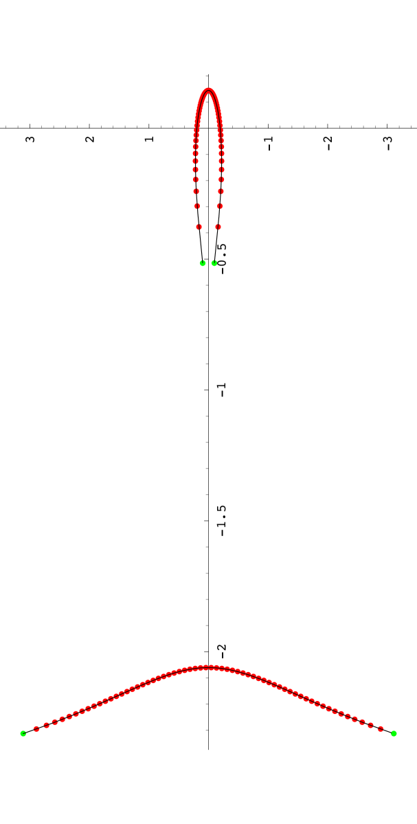
Figure 1: Red dots are the Bethe roots $\mu_{i}$ for the one spin system. Green dots are the branch points. The thin black curve is the solution of eq.(26). ($\hbar=1/30$, $s=1/\hbar$, $M=4/\hbar$, highest energy state).

We can say a word on how the Bethe equations were solved. We first determine $S(\epsilon)$ by solving the polynomial equation eq.(8) and then determine $\psi(z)$, eq.(11), by solving eq.(12). The Bethe roots are then obtained by solving the polynomial equation $\psi(z)=0$.

The idea that the Bethe roots condense in the semi classical limit to form the cuts of the spectral curve goes back to [12]. It plays a very important role in the recent studies on the AdS/CFT correspondence in which it was greatly developed [13, 14]. Eq.(26) however seems to be new.

7 Appendix: The XXX spin chain

In the Gaudin model, the Bethe equations were shown to be equivalent to a Riccati equation eq.(6). Moreover this equation itself determines the parameters $S(\epsilon_{j})$, i.e. the eigenvalues of the commuting Hamiltonians. We show that this construction can be extended to the XXX spin chain.

In the case of the XXX spin chain the Bethe equations take the form (see e.g. [15])

$$\left({\mu_{j}+{i\hbar\over 2}\over\mu_{j}-{i\hbar\over 2}}\right)^{N}=\prod_{k\neq j}{\mu_{j}-\mu_{k}+i\hbar\over\mu_{j}-\mu_{k}-i\hbar}$$ (27)

and the corresponding generating function for the eigenvalues of the commuting Hamiltonians is

$$t(\lambda;\{\mu_{j}\})=\left(\lambda+{i\hbar\over 2}\right)^{N}\prod_{k}{\lambda-\mu_{k}-i\hbar\over\lambda-\mu_{k}}+\left(\lambda-{i\hbar\over 2}\right)^{N}\prod_{k}{\lambda-\mu_{k}+i\hbar\over\lambda-\mu_{k}}$$ (28)

Let us introduce the polynomial

$$Q(\lambda)=\prod_{m=1}^{M}(\lambda-\mu_{m})$$

Then the Bethe equations eq.(27) can be rewritten as

$$\left(\mu_{k}+{i\hbar\over 2}\right)^{N}Q(\mu_{k}-i\hbar)+\left(\mu_{k}-{i\hbar\over 2}\right)^{N}Q(\mu_{k}+i\hbar)=0$$

This means that the polynomial of degree $N+M$

$$\left(\lambda+{i\hbar\over 2}\right)^{N}Q(\lambda-i\hbar)+\left(\lambda-{i\hbar\over 2}\right)^{N}Q(\lambda+i\hbar)$$

is divisible by $Q(\lambda)$. Hence there exists a polynomial $t(\lambda)$ of degree $N$ such that

$$\left(\lambda+{i\hbar\over 2}\right)^{N}Q(\lambda-i\hbar)+\left(\lambda-{i\hbar\over 2}\right)^{N}Q(\lambda+i\hbar)=t(\lambda)Q(\lambda)$$ (29)

This is Baxter’s equation. The polynomial $t(\lambda)$ is the same as in eq.(28) because that equation can be rewritten as

$$t(\lambda;\{\mu_{j}\})=\left(\lambda+{i\hbar\over 2}\right)^{N}{Q(\lambda-i\hbar)\over Q(\lambda)}+\left(\lambda-{i\hbar\over 2}\right)^{N}{Q(\lambda+i\hbar)\over Q(\lambda)}$$

hence the coefficients of this polynomial are the eigenvalues of the set of commuting Hamiltonians.

Just as in the Gaudin model, it is interesting to introduce the Riccati version of eq.(29). We set

$$S(\lambda)={Q(\lambda-i\hbar)\over Q(\lambda)}$$

Then Baxter’s equation becomes

$$\left(\lambda+{i\hbar\over 2}\right)^{N}S(\lambda)+\left(\lambda-{i\hbar\over 2}\right)^{N}S^{-1}(\lambda+i\hbar)=t(\lambda)$$

This equation determines both $S(\lambda)$ and $t(\lambda)$. To find the equation for $t(\lambda)$, we expand around $\lambda=-i\hbar/2$ getting

$$(\epsilon-i\hbar)^{N}S^{-1}(\epsilon+i\hbar/2)=t(\epsilon-i\hbar/2)-\epsilon^{N}S(\epsilon-i\hbar/2)$$

Similarly, expanding around $\lambda=i\hbar/2$ we get

$$(\epsilon+i\hbar)^{N}S(\epsilon+i\hbar/2)=t(\epsilon+i\hbar/2)-\epsilon^{N}S^{-1}(\epsilon+3i\hbar/2)$$

Multiplying the two, we find

$$t\left(\epsilon+{i\hbar\over 2}\right)t\left(\epsilon-{i\hbar\over 2}\right)=(\hbar^{2}+\epsilon^{2})^{N}+O(\epsilon^{N})$$ (30)

This is a system of $N$ equations for the $N+1$ coefficients of $t(\lambda)$ which determines it completely if we remember that $t(\lambda)=2\lambda^{N}+O(\lambda^{N-1})$. Eq.(30) is the characteristic equation of the commuting Hamiltonians of the XXX spin chain.

This construction can be generalized to the case of a spin-s chain. Baxter’s equation reads

$$\left(\lambda+{i\hbar s}\right)^{N}Q(\lambda-i\hbar)+\left(\lambda-{i\hbar s}\right)^{N}Q(\lambda+i\hbar)=t(\lambda)Q(\lambda)$$ (31)

and the Riccati equation becomes

$$\left(\lambda+{i\hbar s}\right)^{N}S(\lambda)+\left(\lambda-{i\hbar s}\right)^{N}S^{-1}(\lambda+i\hbar)=t(\lambda)$$ (32)

Taking $s=1$ for instance, we expand around $\lambda=i\hbar$, $\lambda=0$, $\lambda=-i\hbar$ getting

$$(\epsilon+2i\hbar)^{N}S(\epsilon+i\hbar) = t(\epsilon+i\hbar)+O(\epsilon^{N})$$

$$(\epsilon+i\hbar)^{N}S(\epsilon)+(\epsilon-i\hbar)^{N}S^{-1}(\epsilon+i\hbar) = t(\epsilon)$$

$$(\epsilon-2i\hbar)^{N}S^{-1}(\epsilon) = t(\epsilon-i\hbar)+O(\epsilon^{N})$$

from which we deduce

$$t(\epsilon+i\hbar)t(\epsilon)t(\epsilon-i\hbar)=(\epsilon-i\hbar)^{N}(\epsilon+2i\hbar)^{N}t(\epsilon-i\hbar)+(\epsilon+i\hbar)^{N}(\epsilon-2i\hbar)^{N}t(\epsilon+i\hbar)+O(\epsilon^{N})$$

Clearly for a spin-$s$, $s\geq 0$, the degree of the equation is $2s+1$. If however $s<0$ the equations generically do not lead to a finite degree equation as expected.

In the semi classical limit $\hbar\to 0$, $\hbar s\to s_{cl}$, eq.(32) tends to

$$\left(\lambda+{is_{cl}}\right)^{N}S(\lambda)+\left(\lambda-{is_{cl}}\right)^{N}S^{-1}(\lambda)=t(\lambda)$$

which is nothing but the spectral curve of the classical spin chain.

Acknowledgements. O.B. would like to thank B. Douçot and T. Paul for discussions. The paper was written during the stay of one of the authors (D.T.) at LPTHE in autumn 2006. D.T. would like to thank the French Ambassy in Moscow for organization of this visit. The work of D.T. was supported by the Federal Nuclear Energy Agency of Russia, the RFBR grant 07-02-00645, and the grant of Support for the Scientific Schools 8004.2006.2. The work of O.B. was partially supported by the European Network ENIGMA, MRTN-CT-2004-5652 and the ANR Program GIMP, ANR-05-BLAN-0029-01.

References

- [1] E. Jaynes, F. Cummings, Proc. IEEE vol. 51 (1963) p. 89.
- [2] J. Ackerhalt, K. Rzazewski, Heisenberg-picture operator perturbation theory. Phys. Rev. A, vol. 12, (1975) 2549.
- [3] N. Narozhny, J. Sanchez-Mondragon, J. Eberly, Coherence versus incoherence: Collapse and revival in a simple quantum model. Phys. Rev. A Vol. 23, (1981) p. 236.
- [4] E. Yuzbashyan, V. Kuznetsov, B. Altshuler, Integrable dynamics of coupled Fermi-Bose condensates. cond-mat/0506782
- [5] M. Gaudin, La Fonction d’Onde de Bethe. Masson, (1983).
- [6] E. Mukhin, V. Tarasov, A. Varchenko, The B. and M. Shapiro conjecture in real algebraic geometry and the Bethe ansatz, math.AG/0512299
- [7] E. Sklyanin, Separation of variables in the Gaudin model. J. Soviet Math., Vol. 47, (1979) pp. 2473-2488.
- [8] F. V. Atkinson, Multiparameter spectral theory. Bull. Amer. Math. Soc. 74:1-27 (1968). Multiparameter Eigenvalue Problems. Academic, 1972.
- [9] B. Enriquez, V. Rubtsov, Commuting families in skew fields and quantization of Beauville’s fibration. math.AG/0112276.
- [10] O. Babelon, M. Talon, Riemann surfaces, separation of variables and classical and quantum integrability. hep-th/0209071. Phys. Lett. A. 312 (2003) 71-77.
- [11] D. Talalaev, Quantization of the Gaudin system, hep-th/0404153 Functional Analysis and Its application Vol. 40 No. 1 pp.86-91 (2006)
- [12] N. Reshetikhin and F. Smirnov, Quantum Floquet functions., Zapiski nauchnikh seminarov LOMI (Notes of scientific seminars of Leningrad Branch of Steklov Institute) v.131 (1983) 128 (in russian).
- [13] V. A. Kazakov, A. Marshakov, J. A. Minahan and K. Zarembo, Classical/quantum integrability in AdS/CFT. JHEP 0405 (2004) 024, hep-th/0402207.
- [14] N. Gromov, V. Kazakov, K. Sakai, P. Vieira Strings as Multi-Particle States of Quantum Sigma-Models. Nucl.Phys. B764 (2007) 15-61. hep-th/0603043.
- [15] L.D. Faddeev, How Bethe Ansatz works for integrable models. Les Houches Lectures 1996. hep-th/9605187