ITEP–TH–02/07

hep-th/0703123

February, 2007

Wilson Loops in 2D Noncommutative
Euclidean Gauge Theory:
2. $1/\theta$ Expansion
Jan Ambjørn${}^{a),\;c)}$, Andrei Dubin^b) and Yuri Makeenko${}^{a),\;b)}$

^a)The Niels Bohr Institute,

Blegdamsvej 17, 2100 Copenhagen Ø, Denmark
^b)Institute of Theoretical and Experimental Physics,

B. Cheremushkinskaya 25, 117259 Moscow, Russia
^c)Institute for Theoretical Physics, Utrecht University,

Leuvenlaan 4, NL-3584 CE Utrecht, The Netherlands.

We analyze the $1/\theta$ and $1/N$ expansions of the Wilson loop averages $<W(C)>_{U_{\theta}(N)}$ in the two-dimensional noncommutative $U_{\theta}(N)$ gauge theory with the parameter of noncommutativity $\theta$. For a generic rectangular contour $C$, a concise integral representation is derived (non-perturbatively both in the coupling constant $g^{2}$ and in $\theta$) for the next-to-leading term of the $1/\theta$ expansion. In turn, in the limit when ${\theta}$ is much larger than the area $A(C)$ of the surface bounded by $C$, the large $\theta$ asymptote of this representation is argued to yield the next-to-leading term of the $1/\theta$ series. For both of the expansions, the next-to-leading contribution exhibits only a power-like decay for areas $A(C)>>\sigma^{-1}$ (but $A(C)<<{\theta}$) much larger than the inverse of the string tension $\sigma$ defining the range of the exponential decay of the leading term. Consequently, for large $\theta$, it hinders a direct stringy interpretation of the subleading terms of the $1/N$ expansion in the spirit of Gross-Taylor proposal for the $\theta=0$ commutative $D=2$ gauge theory.

1 Introduction

In short, given a commutative field theory defined in the Euclidean space ${\bf R}^{D}$ by the action $S=\int d^{D}x~{}{\cal L}(\phi(x))$, the corresponding noncommutative theory is implemented replacing the products of the fields $\phi({\bf x})$ by the so-called star-products introduced according to the rule

$$\left(f_{1}\star{f_{2}}\right)({\bf x})\equiv exp\left(-\frac{i}{2}\theta_{\mu\nu}\partial^{y}_{\mu}\partial^{z}_{\nu}\right)~{}f_{1}({\bf y})~{}f_{2}({\bf z})\Bigg{|}_{y=z=x}~{},$$ (1.1)

where the parameter of noncommutativity $\theta_{\mu\nu}$, entering the commutation relation $[x_{\mu},x_{\nu}]=-i\theta_{\mu\nu}$ satisfied by $D$ noncommuting coordinates, is real and antisymmetric. In particular, the action of the standard $D-$dimensional $U(N)$ Yang-Mills theory is superseded by

$$S=\frac{1}{4g^{2}}\int d^{D}x~{}tr\left({\mathcal{F}}^{2}_{\mu\nu}({\bf x})\right)~{}~{}~{}~{};~{}~{}~{}~{}~{}{\mathcal{F}}_{\mu\nu}=\partial_{\mu}{\mathcal{A}}_{\nu}+\partial_{\nu}{\mathcal{A}}_{\mu}-i({\mathcal{A}}_{\mu}\star{\mathcal{A}}_{\nu}-{\mathcal{A}}_{\nu}\star{\mathcal{A}}_{\mu})~{},$$ (1.2)

where ${\mathcal{A}}_{\mu}\equiv{{\mathcal{A}}^{a}_{\mu}t^{a}}$ with $tr(t^{a}t^{b})=\delta^{ab}$, and $\theta_{21}=-\theta_{12}=\theta$ in the $D=2$ case in question.

The noncommutative two-dimensional $U_{\theta}(N)$ system (1.2) provides the simplest example of the noncommutative gauge theory. As well as in the $\theta=0$ case, investigation of non-perturbative effects in a low-dimensional model is expected to prepare us for the analysis of a more complicated four-dimensional quantum dynamics. An incomplete list of papers, devoted to this direction of research, is presented in references [3]-[23].

The aim of the present work is to extend the perturbative analysis of our previous publication [14] and examine, non-perturbatively in the coupling constant $g^{2}$, the two alternative expansions of the Wilson loop-average $<W(C)>_{U_{\theta}(N)}$ in the $D=2$ $U_{\theta}(N)$ theory on a plain. The first one is the $1/\theta$ series

$$<W(C)>_{U_{\theta}(N)}=\sum_{k=0}^{\infty}~{}\theta^{-k}<{\cal W}(C)>^{(k)}_{N}$$ (1.3)

that is to be compared with the more familiar ’t Hooft $1/N$ topological expansion

$$<W(C)>_{U_{\theta}(N)}=\sum_{G=0}^{\infty}~{}N^{-2G}<W(C)>^{(G)}_{U_{\theta}(1)}~{},$$ (1.4)

where $G$ can be identified with the genus of the auxiliary surface canonically associated to any given diagram of the weak-coupling series of the $N-$independent quantity $<W(C)>^{(G)}_{U_{\theta}(N)}$. Also, the contour $C$ is always restricted to be closed.

The $\theta\rightarrow{\infty}$ limit of the $U_{\theta}(N)$ theory is known [24] to retain the same set of the planar diagrams (described by the same amplitudes) as the $N\rightarrow{\infty}$ limit does so that the leading terms of both of the above expansions coincide,

$$<W(C)>^{(0)}_{U_{\theta}(N)}=<{\cal W}(C)>^{(0)}_{N}~{},$$ (1.5)

provided the appropriate identification of the coupling constants. As the $G=0$ term of Eq. (1.4) is $\theta-$independent, it therefore reduces to the corresponding average in the commutative variant of the gauge theory. In consequence, the leading term of the series (1.3) reduces,

$$<{\cal W}(C)>^{(0)}_{N}=<W(C)>^{(0)}_{U(N)}~{}~{}~{}~{}~{},~{}~{}~{}~{}~{}<{\cal W}(\Box)>^{(0)}_{N}=exp[-\sigma A(\Box)]~{},$$ (1.6)

to $G=0$ term of the $\theta=0$ expansion (1.4) of the average $<W(C)>_{U(N)}$ in the ordinary commutative $U(N)$ gauge theory. In particular, it fits in the simple Nambu-Goto pattern for an arbitrary non-self-intersecting contour $C$.

In this paper, for an arbitrary rectangular contour $C=\Box$, we evaluate the next-to-leading term $<W(\Box)>^{(1)}_{U_{\theta}(1)}$ of the topological expansion (1.4) and argue that its large $\theta$ asymptote exactly reproduces,

$$<{\cal W}(C)>_{N}^{(2)}=\frac{1}{N^{2}}~{}\lim_{\theta\rightarrow{\infty}}~{}\theta^{2}<W(C)>_{U_{\theta}(1)}^{(1)}~{},$$ (1.7)

the $k=2$ term $<{\cal W}(\Box)>^{(2)}_{N}$ of the $1/\theta$ series (1.3) (while $<{\cal W}(C)>^{(1)}_{N}=0$). The proof of the relation (1.7) will be presented in a separate publication [25]. As for the computation of $<{\cal W}(C)>_{N}^{(2)}$, for this purpose we perform a resummation of the genus-one diagrams for a generic $C=\Box$, that is facilitated by the choice of the axial gauge where, at the level of the $D=2$ action (1.2), only tree-graphs (without self-interaction vertices) are left. Nevertheless, the problem remains to be nontrivial: due to the noncommutative implementation [26]-[35] of the Wilson loop, an infinite number of different connected $G=1$ diagrams contributes to the average $<W(C)>_{U_{\theta}(N)}$ even in the case of a non-self-intersecting contour $C$ that is in contradistinction with the commutative case, where $<W(\Box)>_{U(N)}=<W(\Box)>^{(0)}_{U(N)}$. To deal with this problem, we propose a specific method of resummation.

Application of the method allows to unambiguously split the whole set of the relevant perturbative $G=1$ diagrams into the three subsets. Being parameterized by the two integer numbers $r$ and $v$ with $0\leq r\leq v\leq 1$, each subset can be obtained starting with the corresponding protograph (with $2+r-v$ lines) and then dressing it through the addition of extra lines in compliance with certain algorithm. For a rectangle $C=\Box$, it yields an integral representation of the $G=1$ term of the $1/N$ expansion in the form

$$<W(\Box)>_{U_{\theta}(1)}^{(1)}~{}=~{}\frac{1}{(2\pi\sigma\theta)^{2}}\sum_{0\leq r\leq v\leq 1}h_{rv}{\cal Z}_{rv}(\bar{A},\bar{\theta}^{-1})~{},$$ (1.8)

where ${\cal Z}_{rv}(\bar{A},\bar{\theta}^{-1})$ denotes the effective amplitude which, after multiplication by the factor $h_{rv}=2+r-v$ separated for a later convenience, accumulates the entire $rv-$subset of the perturbative amplitudes. Besides a dependence on $\bar{\theta}=\sigma\theta$, ${\cal Z}_{rv}(\cdot)$ depends only on the dimensionless area $\bar{A}=\sigma RT$ of $C=\Box$ rather than separately on the lengths $T$ and $R$ of the temporal and spatial sides of $\Box$.

Correspondingly, in the large $\theta$ limit,

$$\theta>>A(C)~{},$$ (1.9)

the $N=1$ relation (1.7) can be rewritten as

$$<{\cal W}(\Box)>_{1}^{(2)}=\frac{1}{(2\pi\sigma)^{2}}\sum_{0\leq r\leq v\leq 1}h_{rv}{\cal Z}_{rv}(\bar{A},0)~{},$$ (1.10)

where ${\cal Z}_{rv}(\bar{A},0)$ is obtained from ${\cal Z}_{rv}(\bar{A},\bar{\theta}^{-1})$ (which is continuous in $\bar{\theta}^{-1}$ in a vicinity of $\bar{\theta}^{-1}=0$) simply replacing $\bar{\theta}^{-1}$ by zero. Then, performing the Laplace transformation with respect to $\bar{A}$, the image $\tilde{\cal Z}_{rv}(\beta,0)$ of the large $\theta$ asymptote ${\cal Z}_{rv}(\bar{A},0)$ assumes the concise form

$$\tilde{\cal Z}_{rv}(\beta,0)=\frac{1}{(\beta+1)^{2}}\int\limits_{-\infty}^{+\infty}d\bar{\zeta}d\bar{\eta}~{}\frac{{\cal K}_{rv}(\bar{\zeta},\bar{\eta})}{(\beta+|1-\bar{\zeta}|)^{h_{rv}-1}~{}(\beta+|1+\bar{\eta}|)~{}(\beta+|1+\bar{\eta}-\bar{\zeta}|)}~{},$$ (1.11)

where

$${\cal K}_{rv}(\bar{\zeta},\bar{\eta})=\sum_{{e}_{3}=-r}^{0}\sum_{{e}_{1}=-1}^{v-r}\sum_{{e}_{2}=v}^{1}(-1)^{v+\sum_{k=1}^{3}{e}_{k}}~{}2^{(v-r)(1-|{e}_{1}|)}|{e}_{1}+\bar{\zeta}|~{}|{e}_{2}+\bar{\eta}|^{1-v}~{}|{e}_{3}+\bar{\zeta}|^{r}~{}.$$ (1.12)

The integral representation (1.11) is the main result of the paper.

Building on the latter representation, one concludes that the pattern of the $\theta\neq{0}$ expansion (1.4) shows, especially in the limit (1.9), a number of features which are in sharp contrast with the $1/N$ expansion of the average in the $\theta=0$ case. Indeed, in the latter case, the Nambu-Goto pattern (1.6) provides the exact result $<W(\Box)>_{U(N)}=<W(\Box)>^{(0)}_{U(N)}$ for an arbitrary non-self-intersecting loop $C$, and the corresponding subleading terms are vanishing: $<W(C)>_{U(N)}^{(G)}=0$ for $G\geq{1}$. Furthermore, for self-intersecting contours $C$, nonvanishing subleading $G\geq{1}$ terms $<W(C)>_{U(N)}^{(G)}$ all possess [36] the area-law asymptote like in Eq. (1.6) in the limit $\bar{A}\rightarrow{\infty}$.

When $\theta\neq{0}$, even for a rectangular loop $C$, the pattern of $<W(C)>_{U_{\theta}(N)}$ is characterized by an infinite $1/N-$series, each $G\geq{1}$ term of which nontrivially depends both on $\bar{\theta}$ and on $\bar{A}(C)$. In addition, we present simple arguments that, in contradistinction with Eq. (1.6), the asymptote (1.10) of the next-to-leading term exhibits a power-like (rather than exponential) decay for areas $\sigma^{-1}<<A(\Box)<<{\theta}$ much larger than the string tension $\sigma$. This asymptote is evaluated in [25] with the result

$$\frac{1}{N^{2}}<W(\Box)>_{U_{\theta}(1)}^{(1)}~{}\longrightarrow~{}\frac{4}{\pi^{2}\left(\sigma\theta N\right)^{2}}~{}\frac{ln(\sigma{A})}{\sigma{A}}~{}~{}~{}~{}~{},~{}~{}~{}~{}~{}\sigma\theta,~{}\sigma{A}~{}\longrightarrow{~{}\infty}~{},$$ (1.13)

that can be traced back to the (infinite, in the limit $\theta\rightarrow{\infty}$) nonlocality of the star-product (1.1) emphasized in the discussion [37] of the $UV/IR$ mixing. Due to the generality of the reasoning, all the subleading $G\geq{1}$ coefficients $<W(C)>_{U_{\theta}(1)}^{(G)}$ are as well expected to show, irrespectively of the form of $C$, a power-like decay for $\sigma^{-1}<<A(C)<<{\theta}$. In particular, it precludes a straightforward stringy interpretation of the subleading terms of the expansion (1.4) in the spirit of Gross-Taylor proposal [38] for the $\theta=0$ commutative $D=2$ gauge theory.

In Section 2, we put forward a concise form (2.10) of the perturbative $2n-$point functions, the loop-average $<W(C)>_{U_{\theta}(1)}$ is composed of in the $D=2$ $U(1)$ theory (1.2). In Section 3, it is sketched how these functions are modified under the two auxiliary (genus-preserving) deformations of a given diagram to be used for the derivation of the decomposition (1.8). To put the deformations into action, in Section 4, we introduce a finite number of the judiciously selected elementary genus-one graphs and propose their $\gamma jrv-$parameterization.

Then, any remaining nonelementary $G=1$ perturbative diagram can be obtained through the appropriate multiple application of the latter deformations to one of thus selected elementary graphs. When a particular elementary diagram with a given $\gamma jrv-$assignment is dressed by all its admissible deformations, the corresponding perturbative $2n-$point function is replaced by the effective one, as it is shown in Section 5. The replacement is implemented in such a way that certain $n-v$ propagators of the are superseded by their effective counterparts (5.7). The integral representation of the effective $2n-$point functions, is completed in Section 6.

In Section 7, we express the $G=1$ term $<W(\Box)>_{U_{\theta}(1)}^{(1)}$ of the expansion (1.4) as a superposition of the effective amplitudes (7.1) that are obtained when the arguments of the above $2n-$point functions are integrated over the rectangle $C=\Box$. The effective amplitudes can be collected into the three $rv-$superpositions ${\cal Z}_{rv}(\bar{A},\bar{\theta}^{-1})$ associated to the corresponding protographs parameterizing the decomposition (1.8). The explicit expression (7.7) for ${\cal Z}_{rv}(\cdot)$ is then derived. It is observed that, for a fixed $rv-$specification, this expression can be deduced directly through the appropriate dressing of the $rv-$protograph. The derivation of the large $\theta$ representation (1.11) is sketched in Section 8. Conclusions, a brief discussion of the perspectives, and implications for $D=3,4$ gauge theory (1.2) are sketched in Section 9. Finally, the Appendices contain technical details used in the main text.

2 Generalities of the perturbative expansion

Building on the integral representation of the $U_{\theta}(1)$ average, we begin with a sketch of the derivation of the relevant perturbative $2n-$point functions.

2.1 Average of the noncommutative Wilson loop

To this aim, consider the perturbative expansion of the average of the noncommutative Wilson loop [26]

$$W(C)={\mathcal{P}}e_{\star}^{i\oint_{C}dx_{\mu}(s){\mathcal{A}}_{\mu}({\bf x}(s))}~{}.$$ (2.1)

in the $U_{\theta}(N)$ noncommutative gauge theory on the 2D plane ${\mathbb{R}^{2}}$. For this purpose, it is sufficient to use the path-integral representation [14] of the $U_{\theta}(1)$ average

$$<W(C)>_{U_{\theta}(1)}=\Bigg{<}exp\left(-\frac{1}{2}\oint\limits_{C}dx_{\mu}(s)\oint\limits_{C}dx_{\nu}(s^{\prime})D_{\mu\nu}({\bf x}(s)-{\bf x}(s^{\prime})+{\bf\xi}(s)-{\bf\xi}(s^{\prime}))\right)\Bigg{>}_{\xi(\tilde{s})}~{},$$ (2.2)

as it follows from the $N-$independence of the quantities $<W(C)>^{(G)}_{U_{\theta}(N)}$ which are, therefore, replaced by $<W(C)>^{(G)}_{U_{\theta}(1)}$ in Eq. (1.4). In Eq. (2.2), $D_{\mu\nu}({\bf z})$ is the standard $D=2$ photon’s propagator in the axial gauge ${\mathcal{A}}_{1}=0$,

$$D_{\mu\nu}({\bf z})=<{\mathcal{A}}_{\mu}({\bf z}){\mathcal{A}}_{\nu}({\bf 0})>_{U(1)}=-\frac{g^{2}}{2}~{}\delta_{\mu 2}\delta_{\nu 2}~{}|z_{1}|~{}\delta(z_{2})~{},$$ (2.3)

and the functional averaging over the auxiliary $\xi_{\mu}(s)$ field (parameterized by the proper time $s\in[0,1]$ chosen to run clockwise starting with the left lower corner of $C=\Box$) is to be performed according to the prescription

$$\Bigg{<}{\mathcal{B}}[{\bf\xi}(s)]\Bigg{>}_{\xi(\tilde{s})}=\int{\mathcal{D}}\xi_{\mu}(s)~{}e^{\frac{i}{2}(\theta^{-1})_{\mu\nu}\int dsds^{\prime}\xi^{\mu}(s)G^{-1}(s,s^{\prime})\xi^{\nu}(s^{\prime})}~{}{\mathcal{B}}[{\bf\xi}(s)]~{}.$$ (2.4)

Here, ${\mathcal{D}}\xi_{\mu}(s)$ denotes the standard flat measure so that $<\xi^{\mu}(s)\xi^{\nu}(s^{\prime})>=i\theta^{\mu\nu}{\rm sign}\,(s-s^{\prime})/2$, where, prior to the regularization, we are to identify $G^{-1}(s,s^{\prime})=\dot{\delta}(s-s^{\prime})$.

Let us also note that Eq. (2.4) is based on the integral representation

$$exp\left(-\frac{i}{2}~{}{\theta}_{\mu\nu}{\partial^{{\bf x}}_{\mu}}{\partial^{{\bf y}}_{\nu}}\right)f_{1}({\bf x})~{}f_{2}({\bf y})=\int e^{2i({\theta}^{-1})_{\mu\nu}\xi_{1}^{\mu}\xi_{2}^{\nu}}f_{1}({\bf x}+{\bf\xi}_{1})f_{2}({\bf y}+{\bf\xi}_{2})~{}\prod_{j=1}^{2}\frac{d^{2}\xi^{\mu}_{j}}{w(\theta)}$$ (2.5)

of the star-product (1.1), where $w(\theta)=(\pi^{2}|\det{\theta}|)^{1/2}$. In consequence, the noncommutative Wilson loop (2.1) itself can be represented as [27],

$$W(C)=\Bigg{<}exp\left(i\oint\limits_{C}dx_{\mu}(s){\mathcal{A}}_{\mu}({\bf x}(s)+{\bf\xi}(s))\right)\Bigg{>}_{\xi(\tilde{s})}~{}.$$ (2.6)

Finally, the coupling $g^{2}$ of the $U_{\theta}(N)$ noncommutative gauge theory is related with the string tension $\sigma$, entering Eq. (1.6), by the formula

$$\sigma=g_{U_{\theta}(N)}^{2}N/2~{}.$$ (2.7)

2.2 Perturbative $\theta$-dependent $2n-$point functions

Take any given $n$th order diagram of the weak-coupling expansion of the average (2.2) that, being applied to the $1/N$ series (1.4) can be rewritten in the form

$$<W(C)>_{U_{\theta}(N)}^{(G)}=\sum_{n=0}^{\infty}\lambda^{2n}~{}<W(C)>_{U_{\theta}(N)}^{(G,n)}$$ (2.8)

with $\lambda=g^{2}N$. For a particular $n\geq 2G$, $<W(C)>_{U_{\theta}(N)}^{(G,n)}$ is given by the multiple contour integral of the $\xi$-average applied to the corresponding product of $n$ $\xi$-dependent propagators $D_{\mu\nu}({\bf y}_{l}+\xi(s_{l})-\xi(s^{\prime}_{l}))$, where

$${\bf y}_{l}={\bf x}(s_{l})-{\bf x}(s^{\prime}_{l})~{},$$ (2.9)

with $l=1,2,...,n$. Then, any diagram can be topologically visualized as the collection of the oriented (according to the proper-time parameterization) lines so that the $q$th propagator-line starts at a given point ${\bf x}(s^{\prime}_{q})\in C$ and terminates at the corresponding ${\bf x}(s_{q})\in C$. When the $\xi$-averaging of the product is performed, the perturbative $2n-$point function can be rewritten [14] in the form

$$V^{(n)}_{U_{\theta}(1)}({\bf y}_{1},...,{\bf y}_{n})=o_{n}~{}\prod_{1\leq l<j}^{n}exp\left(\frac{i}{2}~{}{\cal C}_{lj}\breve{\theta}_{\mu\nu}{\partial^{{\bf z}_{l}}_{\mu}}{\partial^{{\bf z}_{j}}_{\nu}}\right){D}_{22}({\bf z}_{1})~{}{D}_{22}({\bf z}_{2})~{}...~{}{D}_{22}({\bf z}_{n})\Big{|}_{\{{\bf z}_{k}={\bf y}_{k}\}}~{},$$ (2.10)

where $o_{n}=(-1/2)^{n}/n!$, and the intersection matrix ${\mathcal{C}}_{lj}=-{\mathcal{C}}_{ji}$, being defined algebraically as

$${\mathcal{C}}_{lj}=\frac{1}{2}\left(sign(s_{l}-s_{j})+sign(s^{\prime}_{l}-s^{\prime}_{j})-sign(s_{l}-s^{\prime}_{j})-sign(s^{\prime}_{l}-s_{j})\right)~{},$$ (2.11)

counts the number of times the $l$th oriented line crosses over the $j$th oriented line (and, without loss of generality, we presume that $s_{l}\geq s^{\prime}_{l}$ for $\forall{l}$). As for the relevant noncommutative parameter $\breve{\theta}_{\mu\nu}$, it is twice larger

$$\breve{\theta}_{\mu\nu}=2{\theta}_{\mu\nu}~{},$$ (2.12)

compared to the parameter ${\theta}_{\mu\nu}$ defining the original star-product (1.1). Being rewritten in the momentum space, Eq. (2.10) implies that, compared to the commutative case, a given $\theta\neq 0$ perturbative $2n-$point function is assigned with the extra $\theta-$dependent factor

$$\Bigg{<}\prod_{k=1}^{n}e^{i{\bf p}_{k}\cdot({\bf\xi}(s_{k})-{\bf\xi}(s^{\prime}_{k}))}\Bigg{>}_{\xi(\tilde{s})}=exp\left(-i\sum_{l<j}{\mathcal{C}}_{lj}~{}\theta_{\mu\nu}~{}p_{l}^{\mu}~{}p_{j}^{\nu}\right)~{}.$$ (2.13)

where the momentum ${\bf p}_{l}$ is canonically conjugated to the $l$th coordinate (2.9). In turn, the r.h. side of Eq. (2.13) reproduces the existing formula [24, 37] obtained in the analysis of the partition function in the noncommutative field-theories.

Finally, the pattern of Eqs. (2.13) and (2.11) suggests the natural definition of (dis)connected diagrams. Algebraically, a particular $n$th order graph is to be viewed as disconnected in the case when the associated $n\times n$ matrix ${\mathcal{C}}_{lj}$ assumes a block-diagonal form ${\mathcal{C}}_{lj}=\otimes_{k}{\mathcal{C}}^{(k)}_{l_{k}j_{k}}$, with $\sum_{k}n_{k}=n$, so that the nonvanishing entries of ${\mathcal{C}}_{lj}$ are reproduced exclusively by smaller $n_{k}\times n_{k}$ matrices ${\mathcal{C}}^{(k)}_{l_{k}j_{k}}$, where $n_{k}<n$ for $\forall{k}$. Conversely, when a nontrivial implementation of this decomposition of a particular ${\mathcal{C}}_{lj}$ is impossible, the corresponding diagram is called connected. As the rank $r[{\cal C}]=2G(\{{\bf y}_{l}\})$ of the matrix ${\cal C}_{ij}$ is known to be equal to the doubled genus $G(\{{\bf y}_{l}\})$ of the diagram, one expects that the order $n$ of a connected genus $G$ graph complies with the inequality $n(\{{\bf y}_{l}\})\geq{2G(\{{\bf y}_{l}\})}$.

3 The two deformations and the irreducible diagrams

The aim of this Section is to present the central elements of the exact resummation of the weak-coupling series applied to the noncommutative Wilson loop average that, in turn, leads to the decomposition (1.8) introducing the parameters $r$ and $v$. For this purpose, observe first that the complexity of the perturbative expansion of the considered average roots in the complexity of the perturbative $2n-$point functions (2.10) associated to the connected graphs (of an arbitrary large order) discussed in the end of the previous Section. In consequence, for a connected graph of order $m\geq 2G$, the $2m-$point function (2.10) can be expressed in the simplest cases as a multiple irreducible star-product $f_{1}\star{f_{2}}\star...\star{f_{m}}$, where the quantities $f_{k}(\cdot)$ are composed of the propagators (2.3). (In general, the pattern of the connected $2n-$point function can be deduced according to the prescription discussed in the beginning of subsection 3.2.1.) In particular, it can be shown that $2\leq m\leq{3}$ for $G=1$, while Eq. (2.10) for a generic $G=1$ diagram can be represented in the form of an ordinary product of a single $m$th order star-product and a number of the propagators (2.3).

To put this representation into use, we introduce the two genus-preserving deformations to be called ${\cal R}_{a}^{-1}-$ and $\bar{\cal R}_{b}^{-1}-$deformations. Increasing the order $n$ of a $G\geq{1}$ graph by one, they relate the corresponding pairs of functions (2.10) in a way that does not change the multiplicities of all the irreducible star-products involved. Correspondingly, with respect to the inverse ${\cal R}_{a}-$ and $\bar{\cal R}_{b}-$deformations, one introduces ${\cal R}_{a}\otimes\bar{\cal R}_{b}-$irreducible Feynman diagrams.

The advantage of the construction is that nonvanishing amplitudes (2.10) are associated only to the finite number of the irreducible diagrams depicted in figs. 1, 2, 7a, and 7e (which are postulated to fix the topology of the attachment of the lines’ end-points to the upper and lower horizontal sides of $C=\Box$). Then, the complete set of the connected genus-one diagrams can be generated applying all possible $\bar{\cal R}_{b}^{-1}-$deformations to all $m$ lines of these irreducible diagrams. In the end of the Section, we discuss a reason for a further refinement of the resummation algorithm. Being implemented via certain dressing of the lines of the so-called elementary (rather than irreducible) diagrams, the algorithm prescribes that, for any of the dressed lines of the latter diagram, (in the relevant amplitude) one replaces the perturbative propagator by a concise effective propagator (5.7).

3.1 The ${\cal R}_{a}^{-1}-$deformations

The first one is what we call ${\cal R}_{a}^{-1}-$deformation when a given elementary graph is modified by the addition of an extra $i$th propagator-line that does not intersect any line in the original $\{k\}$-set of the elementary diagram:

$${\cal C}_{ik}=0~{}~{}~{}~{}~{}~{}~{}~{},~{}~{}~{}~{}~{}~{}~{}~{}\forall{k\neq{i}}~{}.$$ (3.1)

Starting with a given $2n-$point function $V^{(n)}_{U_{\theta}(1)}(\cdot)$ and identifying $i=n+1$, one readily obtains that, modulo the numerical constant, the considered deformation of $V^{(n)}_{U_{\theta}(1)}(\cdot)$ merely multiplies it by the extra propagator,

$$V^{(n+1)}_{U_{\theta}(1)}({\bf y}_{1},...,{\bf y}_{n},{\bf y}_{n+1})=-\frac{1}{2(n+1)}~{}V^{(n)}_{U_{\theta}(1)}({\bf y}_{1},...,{\bf y}_{n})~{}{D}_{22}({\bf y}_{n+1})~{}.$$ (3.2)

Correspondingly, one defines the inverse of the ${\cal R}_{a}^{-1}-$deformation as the ${\cal R}_{a}-$deformation which eliminates such an $i$th line of a (${\cal R}_{a}-$reducible) diagram that complies with Eq. (3.1) for some $k$. In the absence of such a line (for any $k$), the graph is called ${\cal R}_{a}-$irreducible.

Concerning an $m-$fold application of the ${\cal R}_{a}^{-1}-$deformation, the corresponding generalization of Eq. (3.2) is routine: the single factor $-{D}_{22}({\bf y}_{n+1})/2(n+1)$ is replaced by the product $\prod_{k=1}^{m}(-1){D}_{22}({\bf y}_{n+k})/2(n+k)$. I.e. all of thus generated extra lines are assigned (as well as in the $\theta=0$ commutative gauge theory) with the ordinary perturbative propagator (2.3). For example, a generic non-elementary ${\cal R}_{a}^{-1}-$deformation of the graph in fig. 1a is described by the diagram in fig. 3a. In the latter figure the additional lines are depicted by dotted lines which are vertical (i.e. characterized by vanishing relative time) owing to the pattern of the latter propagator. More generally, the vertical lines in figs. 5, 6, 8, and 9 are also generated by the admissible multiple ${\cal R}_{a}^{-1}-$deformations of the corresponding elementary graphs.

Finally, by the same token as in the $\theta=0$ case, it is straightforward to obtain that the ${\cal R}_{a}^{-1}-$dressing of a given connected graph results in the multiplication of the amplitude, associated to this graph, by a factor to be fixed by Eq. (5.6) below.

3.2 The $\bar{\cal R}_{b}^{-1}-$deformations

The second one is what we denote as the $\bar{\cal R}_{b}^{-1}-$deformation of a given $k$th line of the elementary graph (when the remaining lines of this graph are defined as the $\{q\}_{k}-$set) that introduces an extra line, labeled by $i$, so that the following twofold condition is fulfilled. To begin with, one requires that the $k$th and the $i$th lines, being mutually non-intersecting, intersect the $\{q\}_{k}-$set in the topologically equivalent way (modulo possible reversion of the orientation). E.g. the $\bar{\cal R}_{b}^{-1}-$copies of the right and left solid horizontal lines in fig. 1a are depicted by parallel (owing to the condition (3.7) below) dotted lines in figs. 4b and 4c respectively. In general, it can be formalized by the condition

$${\cal C}_{ik}=0~{}~{}~{}~{}~{},~{}~{}~{}~{}~{}{\cal C}_{iq}=\alpha_{ik}~{}{\cal C}_{kq}~{}~{}~{}~{}~{}~{}~{}~{},~{}~{}~{}~{}~{}~{}~{}~{}\forall{q}\neq{k,i}~{},$$ (3.3)

where, depending on the choice of the relative orientation of the $i$th line, the $q$-independent constant $\alpha_{ik}\equiv{\alpha_{i,k}}$ is equal to $1$ or $-1$ (with $\alpha^{(r)}_{11}=1$). Additionally, it is convenient to impose that thus introduced extra line should not be horizontal, i.e., both its end-points are not attached to the same horizontal side (along the second axis) of the rectangle $C$. As for the inverse transformation, the $\bar{\cal R}_{b}-$deformation deletes such an $i$th line of a diagram that Eq. (3.1) holds true. Correspondingly, any line of a $\bar{\cal R}_{b}-$irreducible graph has no $\bar{\cal R}_{b}^{-1}-$copies in the sense of the above twofold condition.

Next, identifying $\alpha_{n,n+1}=\alpha^{(n)}$, one obtains that the $\bar{\cal R}_{b}^{-1}-$deformation of (2.10) results in the $2(n+1)-$point function

$$V^{(n+1)}_{U_{\theta}(1)}({\bf y}_{1},...,{\bf y}_{n},{\bf y}_{n+1})=$$ (3.4)

$$=o_{n+1}~{}\prod_{1\leq l<j}^{n}e^{\frac{i}{2}~{}{\cal C}_{lj}\breve{\theta}_{\mu\nu}{\partial^{{\bf z}_{l}}_{\mu}}{\partial^{{\bf z}_{j}}_{\nu}}}{D}_{22}({\bf z}_{1})~{}...{D}_{22}({\bf z}_{n-1})\left[{D}_{22}({\bf z}_{n})~{}{D}_{22}(({\bf z}_{n}-{\bf y}_{n})\alpha^{(n)}+{\bf y}_{n+1})\right]\Big{|}_{\{{\bf z}_{k}={\bf y}_{k}\}}~{}.$$

which is expressed through the original $n\times n$ intersection matrix ${\cal C}_{lj}$. In view of the pattern (2.3) of the propagator, Eq. (3.4) implies that

$$\alpha^{(n)}y^{2}_{n}=y^{2}_{n+1}$$ (3.5)

In turn, it entails that the $\bar{\cal R}_{b}^{-1}-$copy of a given line spans the same time-interval (fixed by the second component $y^{2}_{l}$ of the relative distance (2.9)) as the latter line does. In full generality, this property is expressed by Eq. (3.6) that crucially simplifies the computations.

Next, the multiple application of the $\bar{\cal R}_{b}^{-1}-$deformations (3.3), introduces an extra $\{i_{a}\}-$set of the lines which, intersecting nether each other nor the $k$th line, fulfill the $i\rightarrow i_{a}$ option of Eq. (3.3). Then, to reproduce the replacement (5.7), one should take advantage of the following reduction. When applied to an elementary graph, the (multiple) $\bar{\cal R}_{b}^{-1}-$deformations result in diagrams described by vanishing amplitudes unless they are constrained by a particular $\{\alpha^{(r)}\}-$assignment. The amplitude (2.10) may be nonvanishing only when, for any given $r$th line of the elementary graph, all its $\bar{\cal R}_{b}^{-1}-$copies (if any) are assigned with one and the same value of the parameter

$$\alpha^{(r)}_{l1}=\alpha^{(r)}~{}~{}~{}~{}~{},~{}~{}~{}~{}~{}\forall{l}\geq{2}~{},~{}\forall{r}~{},$$ (3.6)

where $\alpha^{(r)}_{lk}=\pm 1$ enters the implementation of Eq. (3.3) corresponding to the $r$th line.

Let us also note that another useful property of the $\bar{\cal R}_{b}^{-1}-$deformations which generalizes the relation (3.5). The corresponding implementations of the $2n-$point function (2.10) enforce that

$$y^{2}_{k}=\alpha^{(k)}_{l1}y^{2}_{k,l}~{}~{}~{}~{}~{},~{}~{}~{}~{}~{}\forall{l=2,...,n_{k}}~{}~{}~{},~{}~{}~{}\forall{k}~{},$$ (3.7)

where ${\bf y}_{k,l}$ denotes the relative distance (2.9) corresponding to the $l$th $\bar{\cal R}_{b}^{-1}-$copy of the $k$th line (described by ${\bf y}_{k}\equiv{\bf y}_{k,1}$). That is why, for $C=\Box$, the latter copies are depicted by such straight dotted lines which are mutually parallel like dotted lines in figs. 4b and 4c.

3.2.1 The necessity for a further refinement

According to above, given a generic connected graph, the pattern of the corresponding $2n-$point function can be deduced from Eq. (2.10) via the replacement ${D}_{22}({\bf z}_{k})\rightarrow{f_{k}({\bf z}_{k},...)}$. Here, $f_{k}({\bf z}_{k},...)$ takes into account possible $\bar{\cal R}_{b}^{-1}-$dressing of the $k$th line of the irreducible diagram (described by the matrix ${\cal C}_{lj}$ of rank $n$) which is associated to the connected graph in question via a sequence of $\bar{\cal R}_{b}-$deformations. Conversely, once a line of an irreducible diagram may be dressed by conglomerates of $\bar{\cal R}_{b}^{-1}-$copies characterized only by an unambiguous value of the corresponding $\alpha^{(k)}$, (in the computation of the amplitude) the overall $\bar{\cal R}_{b}^{-1}-$dressing of this line results in the replacement of the associated perturbative propagator by its effective counterpart to be fixed by the $f_{k}=1$ option of Eq. (5.7).

Still, the shortage of the resummation algorithm, built on the irreducible diagrams, is that some of the time-ordered components of the latter diagrams possess a single line which may be assigned with different signs of $\alpha^{(r)}$. In consequence, the concise prescription of the modification (5.7) of the propagator can not be directly applied to such a line. To circumvent this problem, we use an alternative prescription to reproduce the complete set of the connected $G=1$ diagrams. The idea is to introduce the larger set of the elementary time-ordered graphs (belonging to the three $rv-$varieties in accordance with the decomposition (1.8)) and properly change the algorithm of their $\bar{\cal R}_{b}^{-1}-$dressing so that a single line of some elementary graphs is not dressed at all. As for the overall dressing of each of the remaining lines, being characterized by an unambiguous sign of the corresponding $\alpha^{(k)}$, it is as previously fixed by the $f_{k}=1$ option of the replacement (5.7).

In this way, the set of the genus-one diagrams (generated by the perturbative expansion of the average (2.2)) can be unambiguously decomposed into a finite number of subsets parameterized by the elementary graphs. Then, each subset is described by the associated effective $2n-$point function that, therefore, accumulates the overall ${\cal R}_{a}^{-1}\otimes\bar{\cal R}_{b}^{-1}-$dressing of the corresponding elementary connected $G=1$ graph.

4 The parameterization of the elementary graphs

Let us realize the program formulated in subsection 3.2.1 and introduce such parameterization of the elementary graphs that is as well applicable after the overall ${\cal R}_{a}^{-1}\otimes\bar{\cal R}_{b}^{-1}-$dressing of these graphs. To this aim, the set of the elementary time-ordered graphs is postulated to include not only all time-ordered components of the ${\cal R}_{a}\otimes\bar{\cal R}_{b}-$irreducible Feynman diagrams in figs. 1, 2, 7a, and 7e, but also a variety of a few connected $\bar{\cal R}_{b}-$reducible graphs associated to certain components of the diagrams in figs. 1c and 2e. The additional graphs are obtained from the (time-ordered components of the) diagrams in figs. 7a and 7e via the vertical reattachments applied to the leftmost or/and rightmost end-points of each of the latter diagrams. Preserving both the time-coordinates of the latter end-points and the intersection-matrix (modulo possible change of the sign of its entries), the reattachments replace the single end-point of one or both their horizontal lines from one horizontal side of $C$ to another. Modulo the reflection interchanging the horizontal sides of $C=\Box$, the additional diagrams are depicted in the remaining figs. 7. Note that all these extra diagrams possess exactly one pair of the lines which, being labeled by $i$ and $k$, comply with the condition (3.3). Also, the discussion below implicitly takes into account that both the elementary graphs in the figs. 2a and 2b and all their deformations, being assigned with vanishing amplitudes (2.10), can be therefore excluded from the analysis.

4.1 $S(4)-$symmetry and reflection-invariance

To properly enumerate the elementary graphs and introduce their $\gamma jrv-$parameterization, we should first discuss two types of the transformations which relate the elementary graphs in such a way that the structure of the overall ${\cal R}_{a}^{-1}\otimes\bar{\cal R}_{b}^{-1}-$dressing is kept intact. In turn, to facilitate the application of these transformations, we are to postulate the following convention. When the elementary graphs (or protographs, see subsection 4.2.1) are associated to one and the same time-ordered component of a given Feynman diagram, they are nevertheless considered to be different, provided the topology of the attachment of their lines’ end-points (to the upper and lower horizontal sides of $C=\Box$) is different. For example, the pairs of distinct graphs are depicted in figs. 1a, 1b and figs. 1c, 1d respectively.

Turning to the transformations of the elementary graphs, the first type is implemented through the vertical reattachments which can be combined to generate $S(4)-$multiplets of the latter graphs. Consisting of four graphs, each such multiplet implements the discrete space of the $S(4)-$group of permutations. Note that not only the elementary graphs but also their deformations, included into the subsets described by the corresponding effective amplitudes, are unambiguously splitted into a finite number of distinct (non-overlapping) $S(4)-$multiplets. An example is given by the diagrams in figs. 5c and 6a–6c, where the bold lines depict the associated elementary graph while the nonvertical dotted lines represent the $\bar{\cal R}_{b}^{-1}-$copies introduced by the $\bar{\cal R}_{b}^{-1}-$deformations. As it is illustrated by the latter four figures, the required symmetry of the dressing is maintained by the condition that the positions of the end-points of all the $\bar{\cal R}_{b}^{-1}-$copies are left intact.

As for the second type of the transformations, the $S(4)-$multiplets of the elementary graphs may be related via the $S(2)-$reflection that (mapping the contour $C=\Box$ onto itself) mutually interchanges the two horizontal (or, what is equivalent in the $v=1$ case, vertical) sides of $C$.

Finally, one can implement the $S(4)\otimes S(2)-$transformations to combine the dressed (by all admissible ${\cal R}_{a}^{-1}\otimes\bar{\cal R}_{b}^{-1}-$deformations) elementary graphs into the $S(4)\otimes S(2)-$multiplets. The prescription reads that both the vertical reattachments and the reflections are as previously applied only to the lines associated to the elementary graph, leaving intact the positions of the end-points of all ${\cal R}_{a}^{-1}-$ and $\bar{\cal R}_{b}^{-1}-$copies of these lines. (E.g., figs. 5c, 6a–6c represent the four members of the $S(4)-$multiplet of the dressed graphs to be assigned with $r=v=0$, see below.)

4.2 The $\gamma jrv-$parameterization of the multiplets

Both prior and after their dressing by all admissible ${\cal R}_{a}^{-1}\otimes\bar{\cal R}_{b}^{-1}-$deformations, the elementary graphs are convenient to collect into the $\gamma jrv-$varieties of the $S(4)-$multiplets which consist of $h_{rv}=2+r-v$ $S(4)-$multiplets related via one of the two types of $S(2)-$reflections discussed above. Then, the four integer numbers $\gamma,~{}j,~{}r$, and $v$ parameterize $S(4)\otimes S(2)-$multiplets of the diagrams so that the relevant geometry of the multiple deformations of the graphs in each such multiplet is specified in the reflection- and reattachment-invariant way.

As a result, the algorithm of the resummation can be decomposed into the two steps. At the first step, for given values of $\gamma$, $j$, $r$, and $v$, one constructs the $h_{rv}=2+r-v$ effective amplitudes parameterized by certain special elementary graphs related (when $h_{rv}=2$) via the $S(2)-$reflections. In turn, possessing the maximal number (equal to $h_{rv}$) of the horizontal lines attached to $1+r$ different horizontal sides of $C=\Box$, each of the latter $h_{rv}$ graphs enters the corresponding $S(4)-$multiplet in the $\gamma jrv-$variety. In turn, these are precisely the lines that constitute the associated protograph (relevant for the decomposition (1.8)) which, in the $rv-$variety of the $S(4)-$multiplets (with different $\gamma$ and $j$), has the maximal amount of the horizontal lines. This construction is sketched below (see also Appendix A).

At the second step, the remaining three elementary graphs of each $S(4)-$multiplet (as well as the rest of the protographs) can be then reproduced are obtained via the vertical reattachments of the leftmost or/and rightmost end-points of the above $2+r-v$ horizontal lines. Modulo possible change of the sign of its entries, the intersection-matrix is invariant under these $S(4)-$transformations since, by construction of the elementary graphs, the leftmost and rightmost points of the entire graph necessarily belong to the $h_{rv}$ lines defining the corresponding protograph.

4.2.1 The topological $jrv-$parameterization and the protographs

Consider first the integers $j,~{}r,$ and $v$ which can be interpreted directly in terms of the relevant topological properties common for all the graphs in a given $S(4)-$multiplet. To begin with, $r=0,1$ is equal to the number of the ${\cal R}_{b}^{-1}-$copies of the graph with the maximal number of a single line (to be identified below) available in a given elementary graph. Correspondingly, all the graphs associated to figs. 7 are assigned with $r=1$ (while $v=1$ since $1\geq v\geq{r}$), while the remaining diagrams in figs. 1 and 2, are parameterized by $r=0$.

Next, the number of the lines is equal to $n=1+j+r$. In turn, for a given $r$, $j+1=n-r=2,3$ yields the multiplicity of the irreducible star-product the form of which assumes both the corresponding perturbative $2n-$point function (2.10), and, owing to the replacement (5.7), its effective counterpart considered in subsection 6.1. Therefore, the graphs in figs. 1 and 7a–7d are assigned with $j=1$, while the remaining elementary diagrams are assigned with $j=2$.

As for $v=0,1$ (with $0\leq r\leq v\leq 1$ in compliance with Eq. (1.8)), the $n$th order elementary graph has $h_{rv}=2+r-v$ lines which may be involved into the vertical $S(4)-$reattachments without changing (the module of) the entries of the intersection-matrix. Furthermore, only $2+r-2v$ of these reattached lines are to be dressed, together with the remaining $n-h_{rv}$ lines, by the $\bar{\cal R}_{b}-$copies in compliance with the $f_{k}=1$ prescription (5.7). In particular, for $v=r=1$ graphs of figs. 7, it is the single line, devoid of the latter type of the dressing, that is considered to possess one ${\cal R}_{b}-$copy. (Alternatively, one may state that both the latter line and its copy share the same common $\bar{\cal R}_{b}-$dressing.)

For each of the reattached lines, $2-(v-r)$ of its end-points are $S(4)-$transformed. Therefore, for cases other than $r=1-v=0$, the reattachments can be faithfully represented by the parameters $a_{k}=0,1$ so that $y^{1}_{k}=a_{k}R$, with $k$ assuming $h_{rv}=2$ different values. In the $r=1-v=0$ case (when $h_{rv}=1$), in addition to $a_{1}$ we have to introduce the extra parameter $\tilde{a}_{1}$,

$$x^{1}(s^{\prime}_{1})=(1-a_{1})\tilde{a}_{1}R~{}~{}~{}~{}~{},~{}~{}~{}~{}~{}x^{1}(s_{1})=\tilde{a}_{1}R+(1-\tilde{a}_{1})a_{1}R~{},$$ (4.1)

which is equal to $1$ and $0$ depending on whether or not the reattachment involves the left(most) end-point of the horizontal line of fig. 2e (while $x^{1}(s_{1})-x^{1}(s^{\prime}_{1})=a_{1}R$). To simplify the notations, the pair of the parameters, used to represent the reattachments, is denoted as $\{a_{k}\}\equiv\{a_{k}\}_{rv}$ for all $0\leq r\leq v\leq 1$.

Next, the parameters $r$ and $v$ can be used to enumerate the protographs which are time-ordered as well. A particular protograph, can be reconstructed eliminating all the $n-h_{rv}$ lines of the corresponding elementary graph except for the $2+r-v$ lines affected by the $S(4)-$reattachments. Modulo the $S(4)-$reattachments, thus separated protographs are depicted by bold lines in figs. 3a–3e for those protographs which, for a given $rv-$assignment possess the maximal number $2+r-v$. The figs. 3a, 3b and 3d,3e are in one-to-one correspondence with the pairs of the $S(4)-$multiplets which, being related via the reflection (interchanging the horizontal sides of the contour $C$), are characterized by $r=v=0$ and $r=v=1$ respectively. It should be stressed that, to avoid double-counting, one is to consider only such reflections of the protographs which can not be alternatively reproduced by the vertical $S(4)-$reattachments. Correspondingly, fig. 3c refers to the single $r=v-1=0$ multiplet.

In sum, there are precisely $h_{rv}=2+r-v$ $S(4)-$multiplets of the protographs which, being parameterized by a particular $rv-$assignment, are related via the $S(4)-$reflections. In compliance with Appendix A, in each such multiplet the labels of the $\bar{\cal R}_{b}-$dressed lines assume $n-v=r+j-v+1$ different values in the set $\Omega_{jrv}$ obtained from the sequence $1+v,~{}2,~{}1+j,~{}2+2r$ via the identification of the $v+(2-j)+(1-r)=4+v-n$ coinciding entities (all being equal to 2) so that $n-v=\sum_{k\in{\Omega_{jrv}}}1$. Correspondingly, to parameterize the entire set of $n$ lines, we reliable these lines introducing the the set $\tilde{\Omega}_{jrv}$ obtained from the sequence $1,~{}2,~{}1+j,~{}2+2r$ via the identification of the $(2-j)+(1-r)=4-n$ coinciding entities so that $n=\sum_{k\in\tilde{\Omega}_{jrv}}1$. In turn, the labels of the $2+r-v$ lines, involved into the $S(4)-$reattachments, assume values in the set ${\cal S}_{rv}$ obtained from the sequence $1,~{}c_{rv}=2+3r-v$ (with $c_{rv}=1,2,4$) via the identification of the $v-r$ coinciding entities.

4.2.2 The residual $\gamma-$parameterization of the elementary graphs

The necessity to complete the $jrv-$parameterization and introduce one more parameter $\gamma$, additionally specifying the $S(4)\otimes S(2)-$multiplets, is motivated by the geometry of the pairs of the elementary graphs depicted by bold lines in figs. 8a, 8b (both characterized by $j=r+1=v=1$) and 9a, 9b (both characterized by $j=r=v=1$). In general, with the help of this parameter $\gamma=1,...,f_{jrv}$, one is to enumerate distinct $S(4)\otimes S(2)-$multiplets of the graphs which are separated when one fixes the parameters $j$, $r$, and $v$.

The previous discussion suggests that, to find the number $f_{jrv}$ of such multiplets, it is sufficient to consider only those elementary graphs which, representing the corresponding multiplet, possess the maximal number $h_{rv}$ of the horizontal lines for a particular $jrv-$specification. Then, $f_{jrv}$ is equal to the number of such graphs which, being different time-ordered components of the same Feynman diagram, are not related via the $S(4)\otimes S(2)-$transformations. In turn, the latter number can be found in the following way.

To begin with, for a particular $jrv-$assignment and the matrix ${\cal C}_{ik}$, one fixes generic positions both of the $2+r-v$ horizontal lines (involved into the $S(4)-$reattachments) and of the upper end-points of the remaining $n-(2+r-v)=j-1+v$ nonhorizontal lines. Actually, it is straightforward to infer from Eqs. (3.5) and (3.3) that $f_{jrv}$ is $r-$independent, $f_{jrv}\equiv f_{jv}$, which allows to deduce $f_{jv}$ restricting our analysis the $r=0$ cases. Next, we should take into account that both by the perturbative and the associated effective $2n-$point functions impose $n-2$ specific constraints (see Eq. (5.3) below) on admissible combinations of the temporal components $y^{2}_{l}$ of the relative distances (2.9). In consequence, among the $j-1+v$ lower end-points of the nonhorizontal lines, only $v$ points remain to be independent degrees of freedom (in addition to the $2h_{rv}|_{r=0}+(j-1+v)$ ones already fixed above).

When $v=0$, obviously $f_{j0}=1$ for $j=1,2$. As for $v=1$, when we vary the position of the lower end-point of $k$th nonhorizontal line representing the residual $v=1$ degree of freedom, the resulting time-ordered components of the transformed diagram are distinguished by the $\left[\otimes_{i=1}^{j}Sign(y^{2}_{i})\right]/S(j)-$assignment defined modulo possible $S(j-1+v)-$permutations of the labels $i$ of the $(j-1+v)|_{v=1}$ nonhorizontal lines. Therefore, $f_{j1}=(j-1)+2(2-j)$, where it is formalized that for $f_{11}=(v+1)|_{v=1}$, while $f_{21}=f_{11}-1=1$ (as it is clear from fig. 2e). Summarizing, one arrives at the formula

$$f_{jv}=(1-v)+(3-j)v~{}~{}~{}~{}~{};~{}~{}~{}~{}~{}f_{j0}=f_{2v}=1~{}~{},~{}~{}\forall{j,v}~{},$$ (4.2)

so that $1\leq f_{jv}\leq 2$, and $f_{jv}=2$ only when $j=v=1$.

Note that, although the construction of the parameter $f_{jv}$ is obviously reflection-invariant, the action of the reflections on the $S(4)-$multiplets of the elementary graphs is still nontrivial in the cases when $f_{jv}=2$. The reflections, introduced in subsection 4.2.1, in these cases relate those of the latter multiplets which, being endowed with the same $jrv-$assignment, are described by the two different values of $\gamma$. Summarizing, there are precisely $h_{rv}=2+r-v$ $S(4)-$multiplets of the elementary graphs which, being parameterized by a particular $\gamma jrv-$assignment, are related via the $S(4)-$reflections in the $j-$independent way.

5 Dressing of the elementary graphs and protographs

To derive the representation (1.8), the first step is to express $<W(\Box)>_{U_{\theta}(1)}^{(1)}$ in terms of the $S(4)-$multiplets of the effective $2n-$point functions. Each of these functions describes the corresponding elementary graph together with all its admissible ${\cal R}_{a}^{-1}-$ and $\bar{\cal R}_{b}^{-1}-$deformations according to the algorithm sketched in the previous Section.

In view of the factorization (3.2), for $C=\Box$ it is convenient to represent the effective functions as the product ${\cal I}^{(n)}(\{{\bf y}_{k}\})\tilde{V}_{U_{\theta}(1)}^{(n)}(\{{\bf y}_{k}\})$, where $\{{\bf y}_{k}\}$ denotes the set of the relative coordinates (2.9) characterizing the corresponding time-ordered elementary graph of a given order $2n$. In particular, the factor ${\cal I}^{(n)}(\cdot)$ (to be defined in Eq. (5.6)) accumulates the overall ${\cal R}_{a}^{-1}-$dressing of the latter graph. As for $\tilde{V}_{U_{\theta}(1)}^{(n)}(\cdot)$, it describes a given elementary graph together with the entire its $\bar{\cal R}_{b}^{-1}-$dressing in the way consistent with the $S(4)\otimes S(2)-$symmetry. In turn, the quantity $\tilde{V}_{U_{\theta}(1)}^{(n)}(\cdot)$ can be introduced as the concise modification of the corresponding elementary $2n-$point function (2.10). For this purpose, the perturbative propagators of certain $n-v$ lines should be replaced by the effective ones defined by the $f_{k}=1$ option of Eq. (5.7).

Parameterizing the effective functions, the elementary graphs can be viewed as the intermediate collective coordinates which are useful in the computation of the corresponding individual effective amplitudes

$$\frac{1}{(2\pi\bar{\theta})^{2}}~{}{\cal Z}^{(\gamma)}_{jrv}(\{a_{k}\},\bar{A},\bar{\theta}^{-1})=\oint\limits_{C}\prod_{l=1}^{n}dx^{2}(s_{l})dx^{2}(s^{\prime}_{l})~{}{\cal I}^{(n)}(\{{\bf y}_{k}\})\tilde{V}_{U_{\theta}(1)}^{(n)}(\{{\bf y}_{k}\})\Big{|}^{\gamma}_{jrv}$$ (5.1)

where the vertical $S(4)-$reattachments of the $h_{rv}=2+r-v$ lines are described by the set of the parameters $\{a_{k}\}\equiv\{a_{k}\}_{rv}$ introduced in subsection 4.2.1. By construction, the $G=1$ term $<W(\Box)>_{U_{\theta}(1)}^{(1)}$ of the expansion (1.4) can be represented as the superposition of the amplitudes (5.1) which, as we will see, should be combined into the $rv-$superposition ${\cal Z}_{rv}(\{a_{k}\},\cdot)$. These superpositions are obtained summing up the amplitudes (5.1) corresponding to all $\sum_{j=1}^{2}f_{jv}$ elementary graphs which are associated to a given $rv-$protograph according to the prescription discussed in subsection 4.2.1. Then, Eq. (1.8) is reproduced provided

$${\cal Z}_{rv}(\bar{A},\bar{\theta}^{-1})=\sum_{\{a_{l}\}_{rv}}{\cal Z}_{rv}(\{a_{k}\},\bar{A},\bar{\theta}^{-1})~{}~{}~{}~{}~{},~{}~{}~{}~{}~{}{\cal Z}_{rv}(\{a_{k}\},\bar{A},\bar{\theta}^{-1})=\sum_{j=1}^{2}\sum_{\gamma=1}^{f_{jv}}{\cal Z}^{(\gamma)}_{jrv}(\{a_{k}\},\bar{A},\bar{\theta}^{-1})~{},$$ (5.2)

where $f_{jv}$ is defined in Eq. (4.2), and the sum over $\{a_{l}\}_{rv}$ includes the contribution of the four terms related through the $S(4)-$reattachments applied to the end-points of those lines which, being associated to the corresponding protograph, are parameterized by the label $l\in{\cal S}_{rv}$ (where the set ${\cal S}_{rv}$ is introduced in the end of subsection 4.2.1). In this way, ${\cal Z}_{rv}(\bar{A},\bar{\theta}^{-1})$ yields the contribution of the $S(4)-$multiplet of the protographs endowed with the $rv-$assignment. (Eq. (5.2) takes into account that, when $h_{rv}=2$, the dressed elementary diagrams can be collected into the pairs related via the reflection which leaves the amplitudes ${\cal Z}_{rv}(\bar{A},\bar{\theta}^{-1})$ invariant, as it is verified in Appendix E.)

Then, building on the pattern of the perturbative functions (2.10), the amplitude ${\cal Z}_{rv}(\{a_{k}\},\cdot)$ can be reproduced in a way which reveals the important reduction resulting in the final set of the collective coordinates that, in turn, supports the relevance of the protographs. We postpone the discussion of this issue till subsection 5.3.1.

5.1 Introducing an explicit time-ordering

To proceed further, it is convenient to reformulate both ${\cal I}^{(n)}(\{{\bf y}_{i}\})$ and $\tilde{V}_{U_{\theta}(1)}^{(n)}(\{{\bf y}_{i}\})$ in terms of a minimal amount of independent variable arguments instead of the $n-$set $\{{\bf y}_{i}\}$ of the relative distances (2.9). Consider a rectangular contour $C=\Box$ such that $R$ and $T$ denote the lengths of its vertical and horizontal sides which, in the notations of Eq. (2.3), are parallel respectively to the first and the second axis. Then, the subset $\{y^{1}_{i}\}$ can be reduced to $\{a_{k}\}$, defined after Eq. (5.2). Concerning the reduction of the remaining subset $\{y^{2}_{i}\}$, it can be shown that, among the $\delta-$functional constraints imposed by the $G=1$ effective $2n-$point function $\tilde{V}_{U_{\theta}(1)}^{(n)}(\{{\bf y}_{k}\})$, there are $n-2$ constraints which are the same as in the case of the perturbative $2n-$point function of the associated elementary diagram,

$$\tilde{V}_{U_{\theta}(1)}^{(n)}(\cdot)\sim{V}_{U_{\theta}(1)}^{(n)}(\{{\bf y}_{l}\})\sim\prod_{p=1}^{n-2G}\delta\left(\sum_{l=1}^{n}\lambda^{(p)}_{l}~{}y^{2}_{l}\right)~{},$$ (5.3)

where the $n-2G$ $n$-vectors $\lambda^{(p)}_{l}$, depending only on the topology of the associated elementary graph, span the subspace of those eigenvectors of the intersection matrix ${\mathcal{C}}_{kl}$ which possess vanishing eigenvalue: $\sum_{l=1}^{n}{\mathcal{C}}_{kl}\lambda^{(p)}_{l}=0$ for $p=1,2,...,n-2G$.

In view of the latter constraints imposed on the temporal components $y^{2}_{l}$, there are only $m=n+2$ independent time-ordered parameters $\tau_{k}\geq{\tau_{k-1}}$ which can be chosen to replace the set of the $2n$ temporal coordinates $x^{2}(s_{l})$ and $x^{2}(s^{\prime}_{l})$ assigned to the line’s end-points of a given elementary graph.

Then, as it is shown in Appendix B, there is a simple geometrical prescription to introduce $\tau_{k}$ (with $\tau_{0}=0,~{}\tau_{m+1}=T$). In particular, there are $m-v$ parameters $\tau_{i}$ that are directly identified with the properly associated coordinates $x^{2}(\cdot)$ in the latter $2n-$set. E.g., in the simplest cases to figs. 1a and 2c, the $m$ parameters $\tau_{i}$ simply relabel, according to the relative time-ordering (see Eq. (B.1)), the set of the $m$ end-points attached in these two figures to the upper side of $C=\Box$. Then, combining the $S(4)-$reattachments and the reflection, this prescription can be generalized to deal with the two reflection-pairs of the $r=v=0$ $S(4)-$multiplets of the graphs endowed with $j=1$ and $j=2$. Correspondingly, for $v=1$ in Appendix B we propose, besides $m-1$ such reidentifications associated to certain side of $\Box$, a simple geometrical operation to represent the remaining quantity $\tau_{i_{0}}$ as a superposition of three temporal coordinates $x^{2}(\cdot)$. Furthermore, the proposed $v=1$ prescription can be formulated in the way invariant both under the $S(4)-$reattachments and under the reflection.

Next, on the upper (or, alternatively, lower) horizontal side of the rectangle $C$, $\tau_{q}$ and $\tau_{q-1}$ can be viewed as the bordering points of the $n+3$ connected nonoverlapping intervals

$$\Delta\tau_{k-1}=\tau_{k}-\tau_{k-1}~{}\geq{~{}0}~{}~{}~{}~{}~{},~{}~{}~{}~{}~{}\sum_{k=0}^{m}\Delta\tau_{k}=T~{}~{}~{}~{}~{},~{}~{}~{}~{}~{}m=n+2=j+r+3~{},$$ (5.4)

the overall time $T$ is splitted into. Consequently, the previously introduced relative times

$${t}^{(\gamma)}_{p}\equiv y^{2}_{p}\Big{|}^{\gamma}_{jrv}=(-1)^{s_{p}(\{a_{k}\})}\sum_{l=0}^{m}d^{(\gamma)}_{jrv}(p,l)~{}\Delta{\tau}_{l}~{}~{}~{}~{}~{},~{}~{}~{}~{}~{}d^{(\gamma)}_{jrv}(p,0)=d^{(\gamma)}_{jrv}(p,m)=0~{},$$ (5.5)

can be represented as the superpositions of $\Delta{\tau}_{k}$, and for simplicity we omit the superscript $jrv$ in the notation ${t}^{(\gamma)}_{p}$. In Eq. (5.5), $d^{(\gamma)}_{jrv}(p,l)=0,\pm 1$, while $s(\{a_{k}\})$ denotes an integer-valued $p-$dependent function (fixed by Eq. (E.5) in Appendix E) which additionally depends on the set $\{a_{k}\}$ of the variables introduced after Eq. (4.1).

It is noteworthy that, provided $f_{jv}=2$, the $\gamma-$dependence of ${t}^{(\gamma)}_{p}$ (together with the implicit $\gamma-$dependence of the auxiliary parameter $\omega^{(\gamma)}_{k}$ introduced in Eq. (5.8)) is the only source of the $\gamma-$dependence of the effective amplitude ${\cal Z}^{(\gamma)}_{jrv}(\cdot)$, see Eqs. (6.2) and (6.1) below, associated to the elementary graphs in a $S(4)-$multiplet with a given $\gamma jrv-$assignment. (E.g., the geometry of figs. 8a and 8b implies that $t_{2}^{(1)}<0$ and $t_{2}^{(2)}>0$ respectively.) In turn, the $S(4)-$symmetry of the dressing of the elementary graphs guarantees that the pattern of $t_{p}^{(\gamma)}$ (as well as that of $\omega^{(\gamma)}_{k}$ in Eq. (5.8)) is the same for all members of each $S(4)-$multiplet.

5.2 Accumulating the ${\cal R}_{a}^{-1}-$deformations

Given a particular effective amplitude, the associated ${\cal R}_{a}^{-1}-$deformations a given elementary graph are generated via all possible inclusions of such extra lines that, in accordance with Eq. (3.1), intersect neither each other nor the original lines of the graph. In figs. 3–9 the latter extra lines are depicted as vertical (due to the $\delta-$function in the perturbative propagator (2.3)) and dotted. In view of Eq. (3.2), the inclusion of the deformations of this type merely multiplies the amplitude, describing the original elementary graph, by a factor ${\cal I}^{(n)}(\{{\bf y}_{k}\})$. To deduce this factor, we note that the temporal coordinates of the upper end-points of the ${\cal R}_{a}^{-1}-$copies may span only the first and the last intervals $\Delta\tau_{0}$ and $\Delta\tau_{n+2}$ respectively. Then, akin to the commutative case, it is straightforward to obtain that, when the superposition of all the admissible ${\cal R}_{a}^{-1}-$copies is included, it result in

$${\cal I}^{(n)}(\{{\bf y}_{k}\})=exp\left(-\sigma|R|\left[\Delta\tau_{0}+\Delta\tau_{n+2}\right]\right)~{},$$ (5.6)

the $\tau_{j}-$dependence of which matches the pair of the conditions (5.5) imposed on $d^{(\gamma)}_{jrv}(p,l)$.

5.3 The $\bar{\cal R}_{b}^{-1}-$deformations and the effective propagators

Next, consider the block $\tilde{V}_{U_{\theta}(1)}^{(n)}(\cdot)$ that results after the $\bar{\cal R}_{b}^{-1}-$dressing of a given elementary graph with $n$ lines. The short-cut way to reconstruct this block is to specify those $n-v$ (with $v=0,1$) lines of the latter graph where the corresponding propagator (2.3) is replaced, in the relevant implementation of Eq. (2.10), by its effective counterpart so that the $S(4)-$symmetry of the overall dressing is maintained. When the $k$th line is dressed by all admissible $\bar{\cal R}_{b}^{-1}-$deformations, the replacement is fixed by the $f_{k}=1$ option of the substitution

$${D}_{22}({\bf z}_{k})~{}\longrightarrow~{}\left(-\sigma|z^{1}_{k}|\right)^{f_{k}}\delta\left(z^{2}_{k}\right)~{}exp\left(-\sigma|R+(z^{1}_{k}-y^{1}_{k})\alpha^{(k)}|\Delta T^{b}_{k}(f_{k},\gamma)\right)~{}~{}~{}~{},~{}~{}~{}~{}k\in{\Omega_{2rv}}~{},$$ (5.7)

that reduces to the ordinary multiplication of the propagator ${D}_{22}(\cdot)$ by the $k-$dependent exponential factor (with the set $\Omega_{jrv}$ of the $n-v$ different labels being defined in the end of subsection 4.2.1). In this factor, the parameter $\alpha^{(k)}=\pm 1$ is traced back to Eq. (3.4), and each elementary graph may be endowed only with a single $\{\alpha^{(i)}\}-$assignment (with $i\in{\Omega_{jrv}}$) which renders the global topological characteristic (3.6) of the dressing (5.7) unambiguous. Also,

$$\Delta T^{b}_{k}(f_{k},\gamma)=\Delta\tau_{q(k)}+[1-f_{k}]\Delta\tau_{q(k)+2\omega^{(\gamma)}_{k}-1}~{}~{}~{}~{}~{}~{}~{},~{}~{}~{}~{}~{}~{}~{}~{}\Delta T^{a}_{q}=\Delta\tau_{q}~{}~{},~{}~{}q=0,n+2~{},$$ (5.8)

(i.e., $f_{0}=f_{n+2}=1$), while the extra subscripts $a$ and $b$ are introduced to indicate the type of the associated deformations. In turn, in the $f_{k}=1$ case the interval $\Delta T^{b}_{k}(1,\gamma)=\Delta\tau_{q(k)}$ is spanned by the end-points of the $\bar{\cal R}_{b}^{-1}-$copies of the $k$th line (see Appendix A for particular examples). As for the function $q(k)$ defining the label of the corresponding interval (5.4), it formally determines an embedding of an element of the $S(n-v)$ group of permutations into the $S(n+1)$ group: $0<q(k)<n+2$ for all different $n-v$ values of $k\in{\Omega_{jrv}}$. In Appendix B, we sketch a simple rule which allows to reconstruct $q(k)$ so that this function is common for any given $S(4)-$multiplet of elementary graphs.

5.3.1 The completeness of the $\bar{\cal R}_{b}^{-1}-$dressing of the protographs

To explain the relevance for a certain $f_{k}\neq{1}$ option of the replacement (5.7), we should take into account that, in the evaluation of the amplitude ${\cal Z}_{rv}(\{a_{k}\},\cdot)$ defined by Eq. (5.2), there are important cancellations between the contributions of the individual effective amplitudes (5.1). To obtain ${\cal Z}_{rv}(\{a_{k}\},\cdot)$ for a particular $rv-$assignment, it is sufficient to take the single $j=2$ elementary graph (unambiguously associated to the corresponding protograph) and apply, according to a judicious $\{f_{k}\}-$assignment, the replacement (5.7) to the same $n-v$ lines of this graph as previously. But, contrary to the computation of the amplitudes (5.1), the $f_{k}=1$ variant of the replacement (5.7) remains to be applied only to the $2+r-2v$ lines involved into the $S(4)-$reattachments. The point is that $f_{k}=0$ for all the $(v+j-1)|_{j=2}$ lines which, being not affected by the reattachments (while labeled by $k\in\Omega_{2rv}/{\cal S}_{rv}$, i.e., $k=3$ and, when $v=1$, $k=3-v$), therefore do not belong to the protograph. Furthermore, it is accompanied by such reduction of the measure that, implying the a specific fine-tuning (5.9), retains relevant variable arguments which, at least in the simpler $r=v=0$ case, are associated only to the corresponding protograph. It is further discussed in subsection 7.3, where a more subtle situation for other values of $r$ and $v$ is also sketched.

An explicit ($rv-$dependent) construction of the auxiliary parameters $\omega^{(1)}_{k}=0,1$ with $k=3-v,~{}3$ (and $\gamma=1$ owing to the $j=2$ option of Eq. (4.2)) is presented in subappendix C.1 so that $0<q(k)+2\omega^{(1)}_{k}-1<n+2$, i.e., $\Delta T^{b}_{k}(f_{k},1)\cap\Delta T^{a}_{0}=\Delta T^{b}_{k}(f_{k},1)\cap\Delta T^{a}_{2+n}=0$, $\forall{k\in{\Omega_{2rv}}}$. Then, the emphasized above cancellations result, for any admissible $\{f_{k}\}-$assignment, in the important completeness condition (to be verified in subappendix C.1) fulfilled by the $n-v=\sum_{k\in{\Omega_{2rv}}}1$ intervals $\Delta T^{b}_{k}(f_{k},1)$:

$$\sum_{k\in{\Omega_{2rv}}}\Delta T^{b}_{k}(f_{k},1)=T-\Delta T^{a}_{0}-\Delta T^{a}_{n+2}~{}~{}~{}~{}~{}~{}~{},~{}~{}~{}~{}~{}~{}~{}\sum_{k\in{\Omega_{2rv}}}f_{k}=2+r-2v~{},$$ (5.9)

where each $\Delta T^{b}_{k}(f_{k},1)$ is spanned by the end-points of the $\bar{\cal R}_{b}^{-1}-$copies which, in a given $rv-$protograph, are associated to the $k$th line of the corresponding $j=2$ elementary diagram according to Eq. (7.6). To interpret Eq. (5.9), we first note that the residual time-interval $T-\Delta T^{a}_{0}-\Delta T^{a}_{n+2}$ results from the overall temporal domain $T$ after the exclusion of its left- and rightmost segments $\Delta T^{a}_{0}$ and $\Delta T^{a}_{n+2}$ which (entering the factor (5.6)) are spanned by the end-points of the ${\cal R}_{a}^{-1}-$copies. Also, the $n-v$ open intervals $\Delta T^{b}_{k}(f_{k},1)$ are mutually nonoverlapping, $\Delta T^{b}_{k}(f_{k},1)\cap\Delta T^{b}_{q}(f_{q},1)=0$ for $\forall{k\neq{q}}$, which means that $q(p)\neq q(k)+2\omega^{(1)}_{k}-1$ $\forall{k}\in\Omega_{2rv}/{\cal S}_{rv},~{}\forall{p}\in\Omega_{2rv}$. Then, the completeness condition (5.9) geometrically implies therefore that, once a particular $rv-$protograph is fully dressed, the entire residual time-interval is covered by the $n-v=3+r-v$ mutually nonoverlapping intervals $\Delta T^{b}_{k}(f_{k},1)$. Examples are described by figs. 5c (with $r=v=0$), 8f (with $r=v-1=0$), and 9f (with $r=v=1$).

On the other hand, in the evaluation of the individual effective amplitudes (5.1), the sum in the l.h. side of Eq. (5.9) is replaced by the sum $\sum_{k\in{\Omega_{jrv}}}\Delta\tau_{q(k)}<T-\Delta T^{a}_{0}-\Delta T^{a}_{n+2}$ which generically is less than the residual time-interval. In turn, this inequality follows from the fact that the number $n+1$ of the relevant elementary intervals $\Delta\tau_{k}$ (the residual interval is decomposed into so that $\sum_{i=1}^{n+1}\Delta\tau_{i}=T-\Delta T^{a}_{0}-\Delta T^{a}_{n+2}$) is always less than the number $n-v=\sum_{k\in{\Omega_{2rv}}}1$ of the lines involved into the $f_{k}=1$ dressing (5.7). Examples are presented in the $j=2$ case by figs. 5b, 8c, and 9c.

Finally, in order to introduce and properly utilize the basic formula (6.1) below, in the $v=1$ cases it is convenient to define both $\omega^{(\gamma)}_{k}$ and $\Delta T^{b}_{k}(f_{k},\gamma)$ not only for $j=2$ but for $j=1$ as well. As it is verified in subappendix C.1, the extension is fixed by the prescription: $\omega^{(\gamma)}_{2}|_{j=1}=\omega^{(1)}_{4-\gamma}|_{j=2}$ with $\gamma=1,2$, while $\Delta T^{b}_{k}(f_{k},\gamma)$ is to be defined by the same Eq. (5.8).

6 The structure of the effective amplitude $\tilde{V}_{U_{\theta}(1)}^{(n)}(\{{\bf y}_{k}\})$

The convenient representation (6.1) of the factor $\tilde{V}_{U_{\theta}(1)}^{(n)}(\cdot)$, describing a given $2n$th order elementary graph together with the entire its $\bar{\cal R}_{b}^{-1}-$dressing, can be deduced from the integral representation of the elementary $2n-$point function (2.10) through the simple prescription. For this purpose, the product of the concise exponential factors (6.4) is to be included under the integrand of such representation of the function (2.10) that generalizes Eq. (2.5). In subsection 6.2, we present a brief verification that this prescription matches the result of the appropriate application of the $n-v$ replacements (5.7) with $f_{k}=1$.

6.1 The $\bar{\cal R}_{b}^{-1}-$deformations of the elementary $2n-$point functions

Let us introduce the effective functions $\tilde{V}_{U_{\theta}(1)}^{(n)}(\{{\bf y}_{k}\})$ in a way that makes manifest the relations between those functions which are parameterized by the elementary graphs with a given $rv-$assignment. For this purpose, we first get rid of the $n-2=r+j-1$ $\delta(\cdot)-$functions (defined by the $G=1$ Eq. (5.3)), starting with the $(r+j-1)-$fold integral

$$\int\limits_{-T}^{T}d^{j-1}t^{(\gamma)}_{3}~{}d^{r}t^{(\gamma)}_{4}~{}\tilde{V}_{U_{\theta}(1)}^{(n)}(\{{\bf y}_{k}\})\Big{|}^{\gamma}_{jrv}=J_{jrv}\left[\frac{(-1)^{\omega^{(\gamma)}_{3}-1}\partial}{\partial\tau_{q(3)+\omega^{(\gamma)}_{3}}}\right]^{j-1}\left[\frac{(-1)^{\omega^{(\gamma)}_{2}-1}\partial}{\partial\tau_{q(2)+\omega^{(\gamma)}_{2}}}\right]^{v}\tilde{\cal V}^{(\gamma)}_{jrv}(\{a_{i}\},\{\Delta\tau_{q(k)}\}),$$ (6.1)

where $J_{jrv}=(-1)^{v+j-1}{\sigma^{2+r-v}}/{(2\pi\theta)^{2}}$, $\omega^{(\gamma)}_{k}=0,1$ is introduced in subsection 5.3.1 on the basis of Eq. (5.8), and (for the sake of generality) we temporarily formulate the integration in terms of the relative times (5.5) (rather than $x^{2}(\cdot)$), postulating that $\int d^{0}x\tilde{V}(y)=\tilde{V}(y)$. Then,

$$\tilde{\cal V}^{(\gamma)}_{jrv}(\{a_{i}\},\{\Delta\tau_{q(k)}\})=\int d\zeta d\eta~{}e^{i\left(\eta t^{(\gamma)}_{1}-\zeta t^{(\gamma)}_{2}\right){\cal C}_{21}/\theta}~{}{\cal K}_{rv}(\zeta,\eta,\{a_{i}\})~{}\times$$

$$\times\left[{\cal F}(\alpha^{(1)}\zeta,\Delta\tau_{q(1)})\right]^{1-v}{\cal F}(\alpha^{(2)}\eta,\Delta\tau_{q(2)})~{}\left[{\cal F}(\alpha^{(3)}T_{{\cal C}_{ij}}(\eta,\zeta),\Delta\tau_{q(3)})\right]^{j-1}\left[{\cal F}(\alpha^{(1)}\zeta,\Delta\tau_{q(4)})\right]^{r}~{},$$ (6.2)

with $\alpha^{(k)}$, ${\bf y}_{k}$, ${\cal C}_{ij}$, and $t^{(\gamma)}_{p}$ being given by Eqs. (3.6), (2.9), (2.11), and (5.5) respectively, while

$$\tilde{\cal K}_{rv}(\zeta,\eta,\{a_{i}\})=|a_{1}R+\zeta|~{}|a_{2}R+\eta|^{1-v}|a_{4}R+\alpha^{(1)}\zeta|^{r}~{}~{}~{}~{},~{}~{}~{}~{}y^{1}_{k}=a_{k}R~{},$$ (6.3)

$${\cal F}(\eta,\Delta\tau_{q(k)})=exp\left(-\sigma|R+\eta|\Delta\tau_{q(k)}\right)~{},$$ (6.4)

where $\Delta\tau_{q(k)}$ is the same $k\rightarrow q(k)$ option of the time-interval (5.4) as in the $f_{k}=1$ variant of Eq. (5.7), and

$$T_{{\cal C}_{ij}}(\eta,\zeta)=({\cal C}_{31}/{\cal C}_{21})\eta-({\cal C}_{32}/{\cal C}_{21})\zeta~{},$$ (6.5)

with $|{\cal C}_{21}|=1$.

Finally, Eq. (6.1) is to be augmented by the $r+j-1$ constraints (imposed by thus resolved $\delta-$functions of Eq. (5.3)) that results in the relations

$$(j-1)\left(t^{(\gamma)}_{3}-T_{{\cal C}_{ij}}(t^{(\gamma)}_{2},t^{(\gamma)}_{1})\right)=0~{}~{}~{}~{}~{},~{}~{}~{}~{}~{}r\left(t^{(\gamma)}_{1}-\alpha^{(1)}t^{(\gamma)}_{4}\right)=0~{},$$ (6.6)

where, the second condition yields (when $r=1$) the implementation of the general constraint (3.7), while the first one will be interpreted geometrically in Appendix C. It also noteworthy that the r.h. side of Eq. (6.1) depends on $\gamma$ only through the $\gamma-$dependent quantities $\omega^{(\gamma)}_{p}$ together with the $\gamma-$dependent decomposition (5.5) of the parameters $t^{(\gamma)}_{1}$ and $t^{(\gamma)}_{2}$ entering Eq. (6.2).

6.2 Relation to the elementary $2n-$point functions

Before we discuss how to reinterpret the partial integrand of the effective function (6.1) in compliance with the replacement (5.7), the intermediate step is to establish the relation between the latter function and its counterpart associated to the corresponding elementary graph. Also, we point out a preliminary indication of the relevance of the parameterization in terms of the protographs.

For this purpose, we first take into account that, as it will be proved in Appendix C, in the r.h. side of Eq. (6.1) the partial derivative $\partial/\partial\tau_{q(p)+\omega^{(\gamma)}_{p}}$ acts only on the $p$th factor (6.4) (with $p=3-v,3$) of the expression (6.2). In consequence, these derivatives merely insert, under the integrand, the $r+j-1$ factors $-\sigma|R+{\cal G}_{k}(\zeta,\eta)|$ entering the exponent of Eq. (6.4):

$$\left[\frac{(-1)^{\omega^{(\gamma)}_{3}-1}\partial}{\partial\tau_{q(3)+\omega^{(\gamma)}_{3}}}\right]^{j-1}\left[\frac{(-1)^{\omega^{(\gamma)}_{2}-1}\partial}{\partial\tau_{q(2)+\omega^{(\gamma)}_{2}}}\right]^{v}~{}~{}~{}\longrightarrow~{}~{}~{}(-\sigma)^{j-1+v}|R+T_{{\cal C}_{ij}}(\eta,\zeta)|^{j-1}|R+\eta|^{v}~{},$$ (6.7)

where we have used that $\alpha^{(2)}=1$ when $v=1$, while $\alpha^{(3)}=1$ when $j=2$. Once the replacement (6.7) is performed, the general rule states that, for any admissible $n=1+j+r$, the integral representations of a given elementary $2n-$point function ${V}_{U_{\theta}(1)}^{(n)}(\{{\bf y}_{k}\})$ can be deduced from the corresponding effective one $\tilde{V}_{U_{\theta}(1)}^{(n)}(\{{\bf y}_{k}\})$ through the replacement

$${\cal F}(\cdot,\Delta\tau_{q(k)})~{}\longrightarrow~{}1~{}~{},~{}~{}\forall{k}~{}~{}~{}~{}~{}~{}~{}\Longrightarrow~{}~{}~{}~{}~{}~{}~{}\tilde{V}_{U_{\theta}(1)}^{(n)}(\{{\bf y}_{k}\})~{}\longrightarrow~{}{V}_{U_{\theta}(1)}^{(n)}(\{{\bf y}_{k}\})~{},$$ (6.8)

with ${\cal F}(\cdot)$ being defined by Eq. (6.4). In particular, (provided ${\cal C}_{12}=-1$) the reduced option (6.8) of the $r=v=j-1=0$ implementation of the function (6.1), being associated to the diagrams of fig. 1, assumes the form of integral representation of the $f_{k}({\bf z})\rightarrow D_{22}({\bf z}),~{}k=1,2$ implementation of the star-product (2.5), where the propagator $D_{22}({\bf z})$ is introduced in Eq. (2.3). It is manifest after the identifications: $\zeta\rightarrow{\xi^{1}_{1}},~{}\eta\rightarrow{\xi^{1}_{2}}$. Correspondingly, the $k$th factor $({\cal F}(\cdot,\Delta\tau_{q(k)})-1)$ accumulates the contribution of all admissible $\bar{\cal R}_{b}^{-1}-$copies of the $k$th line so that the interval $\Delta\tau_{q(k)}$ is spanned by the temporal coordinates of the upper (or, equivalently, lower) end-points of the latter copies.

Altogether, in thus reduced Eq. (6.1) the integral representation ${V}_{U_{\theta}(1)}^{(n)}(\{{\bf y}_{k}\})$ of a given $2n$th order elementary graph includes, besides the exponential factor $e^{i\left(\eta t_{1}-\zeta t_{2}\right){\cal C}_{21}/\theta}$ (inherited from Eq. (2.5)) and the $G=1$ product (5.3) of $n-2$ different $\delta(\cdot)-$functions, the product

$$\tilde{\cal K}_{n+2}(\zeta,\eta,R)=\prod_{i=1}^{4}|a_{i}R+{\cal G}_{i}(\zeta,\eta)|^{w_{i}}~{}~{}~{}~{}~{},~{}~{}~{}~{}~{}{\cal G}_{k}(\zeta,\eta)=\tilde{b}_{k}\zeta+\tilde{c}_{k}\eta~{},$$ (6.9)

composed of $n=1+j+r$ factors $|a_{i}R+{\cal G}_{i}(\zeta,\eta)|$ each of which represents (when $w_{i}\neq{0}$, i.e., for $i\in\tilde{\Omega}_{jrv}$) the $i$th propagator of the latter graph so that $w_{1}=w_{2}=1,~{}w_{3}=j-1=0,1,~{}w_{4}=r=0,1$ with $\sum_{i=1}^{4}w_{i}=n$. Here, $a_{k}$ is defined in Eq. (6.3), $\tilde{b}_{q},\tilde{c}_{q}=0,\pm 1$, while $R$ is defined in the footnote prior to Eq. (4.1), and $2\leq n\leq 4$. In turn, it is the $\tilde{\cal K}_{rv}(\cdot)-$part (6.3) of $\tilde{\cal K}_{n+2}$ which, being associated to the $2+r-v$ lines involved into the $S(4)-$reattachments (when $a_{k}$ assumes both of the admissible values), refers to the protographs. The remaining $v+j-1$ lines, corresponding to the $f_{k}=0$ option of the replacement (5.7), are not affected by the reattachments so that the corresponding $a_{k}$ are equal to unity which matches the $a_{k}=1$ pattern of the exponents (6.4) necessarily associated to all these lines via the replacement (6.7).

In conclusion, it is routine to convert the inverse of the prescription (6.8) into the composition of the replacements (5.7). In view of Eq. (6.7), the general pattern (6.1) is such that any particular effective $2n-$point function $\tilde{V}_{U_{\theta}(1)}^{(n)}(\{{\bf y}_{k}\})$ can be deduced from the associated elementary one through the corresponding option of the replacement

$$\prod_{k=1}^{4}|a_{k}R+{\cal G}_{k}(\zeta,\eta)|^{w_{k}}~{}\longrightarrow~{}\prod_{k=1}^{4}|a_{k}R+{\cal G}_{k}(\zeta,\eta)|^{w_{k}}~{}e^{-\sigma v_{k}|R+{\cal G}_{k}(\zeta,\eta)\alpha^{(k)}|\Delta\tau_{q(k)}}~{},$$ (6.10)

where $v_{1}=1-v=0,1$, $v_{k}=w_{k}$, for $k=2,3,4$ (with $v_{k}\neq 0$ only when $k\in\Omega_{jrv}$, $\sum_{k=1}^{4}v_{i}=n-v$) that matches the pattern of Eq. (6.2). Then, it takes a straightforward argument to verify that the substitution (6.10) is indeed equivalent to the $f_{k}=1$ prescription (5.7) applied, with the identification $\alpha^{(4)}=\alpha^{(1)}$, to the corresponding $\Omega_{jrv}-$subset of the $n-v$ perturbative propagators.

7 Integral representation of the effective amplitudes

At this step, we are ready to obtain the explicit form of the amplitude ${\cal Z}_{rv}(\bar{A},\bar{\theta}^{-1})$ which, being introduced in Eq. (5.2), defines the decomposition (1.8) of the $G=1$ term $<W(\Box)>_{U_{\theta}(1)}^{(1)}$ of the $1/N$ expansion (1.4). For this purpose, we first put forward the general representation (7.1) of the individual effective amplitudes (5.1) which, being parameterized by the corresponding elementary graphs, are evaluated non-perturbatively both in $g^{2}$ and in $\theta$. The latter amplitudes arise when the $2n-$point function $\tilde{V}_{U_{\theta}(1)}^{(n)}(\{{\bf y}_{k}\})$, being multiplied by the factor (5.6), is integrated over the $n$ pairs of the relative coordinates (2.9) (defining the set $\{{\bf y}_{k}\}$), all restricted to the contour $C=\Box$.

Then, building on this representation, the superposition (5.2) of ${\cal Z}^{(\gamma)}_{jrv}(\cdot)$ is evaluated collecting together the contributions associated to all the elementary graphs with the same $rv-$assignment. In turn, the specific cancellations, taking place between the different terms of the superposition, support the pattern of the relevant collective coordinates. In particular, it verifies the representation of $\tilde{V}_{U_{\theta}(1)}^{(n)}(\cdot)$ (discussed in subsection 5.3.1) formulated in terms of the properly dressed protographs. We also clarify the relation between the latter dressing and the structure of the collective coordinates.

7.1 General pattern of the individual effective amplitudes

Synthesizing the factors (5.6) and (6.1), one concludes that the individual effective amplitudes (5.1) assume the form

$$(-1)^{\sum_{l\in{\cal S}_{rv}}a_{l}}~{}{\cal Z}^{(\gamma)}_{jrv}(\{a_{k}\},\bar{A},\bar{\theta}^{-1})=$$

$$=\bar{A}^{2+h_{rv}}\int d^{n+2}\bar{\tau}e^{-\bar{A}\left(\Delta\bar{\tau}_{0}+\Delta\bar{\tau}_{n+2}\right)}\left[\frac{(-1)^{\omega^{(\gamma)}_{3}-1}\partial}{\partial\tau_{q(3)+\omega^{(\gamma)}_{3}}}\right]^{j-1}\left[\frac{(-1)^{\omega^{(\gamma)}_{2}-1}\partial}{\partial\tau_{q(2)+\omega^{(\gamma)}_{2}}}\right]^{v}{\cal V}^{(\gamma)}_{jrv}(\{a_{i}\},\{\Delta\bar{\tau}_{q(k)}\}),$$ (7.1)

where the sum in the l.h. side runs over the labels $l$ of the $2+r-v$ lines involved into the $S(4)-$reattachments in the first relation of Eq. (5.2) (with the set ${\cal S}_{rv}$ being specified in the end of subsection 4.2.1), and we introduce the compact notation

$$\int\limits_{0\leq\bar{\tau}_{k}\leq\bar{\tau}_{k+1}}^{\bar{\tau}_{m}\leq 1}\prod_{l=1}^{m}d\bar{\tau}_{l}...\equiv\int d^{m}\bar{\tau}...~{},$$ (7.2)

for the integrations over the $m=n+2$ ordered times $\bar{\tau}_{j}$, and, for a rectangular contour $C=\Box$ of the size $R\times T$, it is convenient to utilize the change of the variables

$$\tau_{k}=T\bar{\tau}_{k}~{}~{}~{}~{}~{},~{}~{}~{}~{}~{}t_{k}=T\bar{t}_{k}~{}~{}~{}~{}~{},~{}~{}~{}~{}~{}\zeta=R\bar{\zeta}~{}~{},~{}~{}\eta=R\bar{\eta}~{},$$ (7.3)

which introduces the dimensionless quantities $\bar{\tau}_{k}$ (with $\Delta\bar{\tau}_{k-1}=\bar{\tau}_{k}-\bar{\tau}_{k-1}\geq{0}$), $\bar{\eta}$, $\bar{\zeta}$, and $\bar{t}_{k}$ so that $R^{4+r-v}{\cal V}_{jrv}(\{a_{i}\},\{\Delta\bar{\tau}_{q(k)}\})=\tilde{\cal V}_{jrv}(\{a_{i}\},\{T\Delta\bar{\tau}_{q(k)}\})$. In particular, this change makes it manifest that, besides the dependence on $\{a_{i}\}$ and $\bar{\theta}=\sigma\theta$, the considered effective amplitudes are certain functions of the dimensionless area of the rectangle $C$

$$\bar{A}=\sigma A(C)\Big{|}_{C=\Box}=\sigma RT$$ (7.4)

rather than of $R$ and $T$ separately.

Note also that in the r.h. side of Eq. (7.1) the $m=n+2$ species of the $d\bar{\tau}_{j}-$integrations reproduce, according to the discussion of subsection 5.1, the $2n-$fold contour-integral (5.1) which runs over the time-coordinates $dx^{2}(s_{l})$ and $dx^{2}(s^{\prime}_{l})$ constrained by the $G=1$ product (5.3) of the $\delta(\cdot)-$functions. Correspondingly, this transformation of the measure has the jacobian which is equal to $(-1)^{n_{jrv}^{-}}$, where $n_{jrv}^{-}$ and $n_{jrv}^{+}$ denote the numbers of the line’s end-points attached, for a given elementary graph, respectively to the lower and upper horizontal side of the rectangle $C=\Box$ so that

$$(-1)^{n_{jrv}^{-}}=\prod_{i\in\tilde{\Omega}_{jrv}}(-1)^{a_{i}}~{}~{}~{}~{}~{}~{}~{},~{}~{}~{}~{}~{}~{}~{}\frac{1}{2}(n_{jrv}^{+}+n_{jrv}^{-})=n_{jrv}\equiv n=\sum_{k\in\tilde{\Omega}_{jrv}}1~{},$$ (7.5)

where $a_{k}$ is defined in Eq. (6.3), while the set $\tilde{\Omega}_{jrv}$ is specified in the end of subsection 4.2.1. In turn, to justify the $\{a_{k}\}-$dependent sign-factor in the l.h. side of Eq. (7.1), it remains to notice that $\sum_{k\in\tilde{\Omega}_{jrv}}a_{k}=v+j-1+\sum_{l\in{\cal S}_{rv}}a_{l}$ since $a_{k}=1$ for $\forall{k}\in\tilde{\Omega}_{jrv}/{\cal S}_{rv}$.

7.2 Derivation of the combinations ${\cal Z}_{rv}(\bar{A},\bar{\theta}^{-1})$

The effective amplitudes (7.1), parameterized by the individual elementary graphs, are still intermediate quantities. To say the least, for generic $\bar{A}$, they are singular for $\bar{\theta}^{-1}\rightarrow{0}$. To arrive at amplitudes which are already continuous in $\bar{\theta}^{-1}$ in a vicinity of $\bar{\theta}^{-1}=0$, our aim is to evaluate the combinations (5.2) of the latter amplitudes entering the decomposition (1.8).

Then, to reveal the cancellations between different terms of the sum (5.2), in the r.h. side of Eq. (7.1) one is to perform $v+j-1$ integrations to get rid of the corresponding number of the partial derivatives (employing that $0<q(k)<n+2$ for $\forall{k}=1,..,n$). In Appendix C, it is shown that, matching the prescription (5.7) formulated in subsection 5.3.1, a straightforward computation yields

$${\cal Z}_{rv}(\bar{A},\bar{\theta}^{-1})=\bar{A}^{2+h_{rv}}\sum_{\{a_{l}\}_{rv}}(-1)^{\sum_{l\in{\cal S}_{rv}}a_{l}}\int d^{2+h_{rv}}\bar{\tau}~{}e^{-\bar{A}\left(\Delta\bar{\tau}_{0}+\Delta\bar{\tau}_{2+h_{rv}}\right)}~{}{\cal V}_{2rv}(\{a_{k}\},\{\Delta\bar{T}^{b}_{k}\})~{},$$ (7.6)

where the sum over $a_{l}$ is the same as in Eq. (5.2), $\tilde{\cal V}_{2rv}(\cdot)\equiv{\tilde{\cal V}^{(1)}_{2rv}(\cdot)}$ is defined in Eq. (6.2), and we have omitted the subscript $\gamma=1$ since, in view of Eq. (4.2), $\gamma$ assumes the single value for $j=2$ irrespectively of the values of $r$ and $v$. Note that, in the exponent, $\Delta\bar{\tau}_{n+2}$ is replaced by $\Delta\bar{\tau}_{2+h_{rv}}\equiv T^{-1}\Delta T^{a}_{2+h_{rv}}$ while, in the quantity ${\cal V}_{2rv}(\cdot,\cdot)$, the set $\{\Delta\bar{\tau}_{q(k)}\}$ is superseded by $\{\Delta\bar{T}^{b}_{k}\}\equiv\{\Delta\bar{T}^{b}_{k}(f_{k},1)\}$, where the intervals $\Delta\bar{T}^{b}_{k}(f_{k},1)=T^{-1}\Delta T^{b}_{k}(f_{k},1)$, being constrained by the condition (5.9), are introduced in Eq. (5.8). Altogether, omitting the subscripts $a$ and $b$, the relevant $3+h_{rv}$ intervals $\Delta\bar{T}_{i}=\bar{\tau}_{i+1}-\bar{\tau}_{i}\geq 0$ are expressed through $2+h_{rv}$ ordered quantities $\bar{\tau}_{i}$ characterized by the $m=2+h_{rv}$ option of the measure (7.2).

Finally, according to Appendices D and E, the r.h. side of Eq. (7.6) can be rewritten in the form

$${\cal Z}_{rv}(\bar{A},\bar{\theta}^{-1})=\bar{A}^{2+h_{rv}}\int d^{2+h_{rv}}\bar{\tau}\int\limits_{-\infty}^{+\infty}d\bar{\zeta}d\bar{\eta}~{}e^{i\left(\bar{\eta}\bar{t}_{1}-\bar{\zeta}\bar{t}_{2}\right)\bar{A}/\bar{\theta}}~{}{\cal K}_{rv}(\bar{\zeta},\bar{\eta})~{}{\cal Y}_{rv}(\bar{\zeta},\bar{\eta},\{\Delta\bar{\tau}_{k}\}),$$ (7.7)

where $\bar{t}_{p}\equiv\bar{t}^{(1)}_{p}$, $p=1,2$,

$${\cal Y}_{rv}(\cdot)=e^{-\bar{A}\left(\Delta\bar{\tau}_{0}+\Delta\bar{\tau}_{2+h_{rv}}\right)}~{}exp\left(-\bar{A}\left[(1+r-v)|1-\bar{\zeta}|\Delta\bar{\tau}_{3}+|1+\bar{\eta}|\Delta\bar{\tau}_{1+v}+|1-\bar{\zeta}+\bar{\eta}|\Delta\bar{\tau}_{2-v}\right]\right)~{},$$ (7.8)

${\cal K}_{rv}(\cdot)$ is given by Eq. (1.12), and the sum over $\{e_{k}\}$ supersedes the one over $\{a_{l}\}_{rv}$ (combining four different implementations ${\cal Z}_{rv}(\{a_{k}\},\cdot)$) so that the dressing-weight ${\cal Y}_{rv}(\cdot)$ is manifestly $S(4)-$invariant, i.e., $\{e_{k}\}-$independent. For the particular $\{a_{k}\}-$assignments, ${\cal Z}_{rv}(\{a_{k}\},\cdot)$ is diagrammatically depicted in figs. 5c ($a_{1}=a_{2}=0$), 8f ($a_{1}=0$), and 9f ($a_{1}=a_{4}=0$) which are associated to $r=v=0$, $r=v-1=0$, and $r=v=1$ respectively.

Let us also note that the representation (7.7) readily allows to demonstrate that, for $\forall{\bar{A}}>0$, ${\cal Z}_{rv}(\bar{A},\bar{\theta}^{-1})$ is indeed continuous in $\bar{\theta}^{-1}$ in a vicinity of $\bar{\theta}^{-1}=0$. This property, implied in the transformation of Eq. (1.8) into Eq. (1.10), will be explicitly derived in [25].

7.3 A closer look at the pattern of the collective coordinates

In conclusion, let us clarify the following subtlety concerning the pattern of the collective coordinates relevant for the dressing of the $rv-$protograph. The point is that, in the $v=1$ Eq. (7.7), both the measure $d^{2+h_{rv}}\bar{\tau}$ and the relative time $\bar{t}_{2}\equiv\bar{t}^{(\gamma)}_{2}$ can not be fully determined only on the basis of the configuration of the $rv-$protograph itself (postulated to be constrained, in the $r=1$ case, by the second of the conditions (6.6)). The general reason is traced back to the fact that the $v=1$ protographs are not of genus-one and, therefore, their dressing necessarily encodes certain structure inherited from the associted $j=2$ elementary diagrams.

In consequence, the above measure includes integration over one more parameter $\bar{\tau}_{2+r}$ in addition to the $2h_{rv}-r=2-v+h_{rv}$ parameters which are directly identified (see Appendices C and B for the details), with the independent temporal coordinates of the end-points of the protographs’ lines:

$$\int d^{2+h_{rv}}\bar{\tau}~{}...=\int d^{2-v+h_{rv}}\bar{\tau}\int d^{v}\bar{t}_{2}...~{},$$ (7.9)

where we have used that $\bar{t}_{2}=\bar{\tau}_{2+r}-\bar{\tau}_{1}$ (with $\tau_{1}=x^{2}(s^{\prime}_{1})$ as it is depicted in figs. 8f and 9f). Then, as it is discussed in Appendix B, the presence of $\tau_{2+r}$ is tightly related to the first of the constraints (6.6) fulfilled by the three parameters $t_{p},~{}p=1,2,3$. In turn, as it is sketched in Appendix C, the latter constraints underlie the completeness condition (5.9) for $\forall{r,v}$.

Note also the reduction $\int d^{2+n}\bar{\tau}~{}..\rightarrow\int d^{4+r-v}\bar{\tau}~{}..$ of the relevant measure, formalized by the transition from the combination of the individual amplitudes (7.1) to Eq. (7.6), entails the relevant $f_{k}=0$ replacements (5.7) applied to the $j=2$ Eq. (7.1). Indeed, the latter replacements result after such integration over $n-(2+r-v)|_{j=2}=v+1$ parameters $\tau_{q(p)+\omega^{(\gamma)}_{p}}$ (with $p=3-v,3$), in the process of which the corresponding intervals $\Delta\tau_{q(k)}$ vary in the domains $[0,\Delta T^{b}_{k}(0,\gamma)]$ (see Appendix C for more details).

8 The large $\theta$ limit

At this step we are ready to put forward the prescription (8.1) to implement the large $\theta$ limit in Eq. (7.7). By virtue of the $1/\theta^{2}$ factor in front of the sum in the r.h. side of eq. (1.10), the asserted large $\theta$ scaling $<W(\Box)>_{U_{\theta}(1)}^{(1)}\sim\theta^{-2}$ is a consequence of the important property of the combinations ${\cal Z}_{rv}(\bar{A},\bar{\theta}^{-1})$. For any finite $\bar{A}\neq 0$, the relevant large $\theta$ limit (1.9) can implemented directly through the substitution

$$e^{i\left(\bar{\eta}\bar{t}_{1}-\bar{\zeta}\bar{t}_{2}\right)\bar{A}/\bar{\theta}}~{}\longrightarrow~{}1~{}~{}~{}\Longrightarrow~{}~{}~{}{\cal Z}_{rv}(\bar{A},\bar{\theta}^{-1})~{}\longrightarrow~{}{\cal Z}_{rv}(\bar{A},0)~{},$$ (8.1)

to be made in the integrand of the representation (7.7) of the quantity ${\cal Z}_{rv}(\bar{A},\bar{\theta}^{-1})$ that replaces the latter quantity by its reduction ${\cal Z}_{rv}(\bar{A},0)$. In turn, provided Eq. (1.7) is valid, the prescription (8.1) yields the integral represetation (1.10) for the next-to-leading term of the $1/\theta$ expansion (1.3) (with $<{\cal W}(\Box)>_{N}^{(1)}=0$).

The self-consistency of the deformation (8.1) is maintained provided ${\cal Z}_{rv}(\bar{A},\bar{\theta}^{-1})$ is continuous in $\bar{\theta}^{-1}$ in a vicinity of $\bar{\theta}^{-1}=0$. In turn, it can be shown that, for $\bar{A}\neq 0$, the latter property is valid provided this deformation does not violate the convergence of the $(m+2)-$dimensional integral over $\bar{\tau}_{k}$, $\bar{\zeta}$, and $\bar{\eta}$ defining the representation (7.7) of ${\cal Z}_{rv}(\bar{A},\bar{\theta}^{-1})$, where $m=2+h_{rv}$. To demonstrate the convergence, it is convenient first to get rid of the explicit $m-$dimentional ordered integration over $\bar{\tau}_{j}$. For this purpose, it is useful to perform the Laplace transformation of ${\cal Z}_{rv}(\bar{A},\bar{\theta}^{-1})$ with respect to the dimensionless area (7.4) that results in

$$\tilde{\cal Z}_{rv}(\beta,\bar{\theta}^{-1})=\int_{0}^{+\infty}d\bar{A}~{}{\cal Z}_{rv}(\bar{A},\bar{\theta}^{-1})~{}e^{-\beta\bar{A}}~{}.$$ (8.2)

The advantage of this trick is that, in the integral representation of the image $\tilde{\cal Z}_{rv}(\beta,\bar{\theta}^{-1})$, the $\bar{\tau}_{j}-$integrations can be easily performed using the general relation

$$\prod_{j=0}^{m}\frac{1}{\beta+B_{j}}=\int\limits_{0}^{+\infty}d\bar{A}~{}e^{-\beta\bar{A}}\int\limits_{0\leq\breve{\tau}_{k}\leq\breve{\tau}_{k+1}}^{\breve{\tau}_{m}\leq\bar{A}}\prod_{k=1}^{m}d\breve{\tau}_{k}\prod_{j=0}^{m}exp\left(-B_{j}\Delta\breve{\tau}_{j}\right)~{},$$ (8.3)

where $\breve{\tau}_{j}$ is to be identified with $\bar{A}\bar{\tau}_{j}$, while $\Delta\breve{\tau}_{j-1}=\breve{\tau}_{j}-\breve{\tau}_{j-1}$ with $\breve{\tau}_{0}\equiv{0}$ and $\breve{\tau}_{m+1}\equiv{\bar{A}}$. In particular, in this way one proves that the Laplace image $\tilde{\cal Z}_{rv}(\beta,0)$ of the large $\theta$ asymptote ${\cal Z}_{rv}(\bar{A},0)$ of the amplitude (7.7) assumes the form (1.11).

As for the self-consistency of the prescription (8.1), it can be verified provided the double integral (1.11) is convergent for $\forall{\beta}>0$ so that $\tilde{\cal Z}_{rv}(\beta,\bar{\theta}^{-1})$ is continuous in $\bar{\theta}^{-1}$ in a vicinity of $\bar{\theta}^{-1}=0$. A direct inspection verfies that the convergence indeed takes place.

Also, it should be stressed that, due to the infrared singularities of the propagators, the prescription (8.1) is not applicable directly to each individual perturbative diagram. This property may be inferred from the integral representations of the elementary amplitudes given by the reduction (6.8) of the effective amplitudes considered in subsection 6.1. Actually, even the individual effective amplitudes (7.1) still are not suitable for this purpose either that can be traced back to the violation of the completeness condition (5.9). It takes certain specific cancellations between the latter amplitudes that, resulting in the latter condition, makes the substitution (8.1) applicable to the combinations (7.7). We shall continue the discussion of this issue in [25].

9 Conclusions

In the present paper we obtain the exact integral representation (1.8) of the next-to-leading term $<W(\Box)>_{U_{\theta}(1)}^{(1)}$ of the $1/N$ expansion (1.4) of the average in the $D=2$ gauge theory (1.2). It provides the rigorous non-perturbative computation made, from the first principles, in the noncommutative gauge theory.

The Laplace image (8.2) of the large $\theta$ asymptote of $<W(\Box)>_{U_{\theta}(1)}^{(1)}$ assumes the particularly concise form (1.10). In turn, the latter asymptote is argued to be directly related (1.7) to the next-to-leading term of the $1/\theta$ expansion (1.3) of $<W(C)>_{U_{\theta}(1)}$. It is noteworthy that the considered asymptote reveals the power-like decay which is in sharp contrast with the exponential area-law asymptote (1.6) valid in the leading order of the $1/N-$ (or, equivalently, $1/\theta-$) expansion. Furthermore, as the origin of the power-like decay can be traced back to the (infinite, in the limit $\theta\rightarrow{\infty}$) nonlocality of the star-product, similar decay is supposed to persist for all $G\geq{1}$ subleading terms $<W(C)>_{U_{\theta}(1)}^{(G)}$ of the large $\theta$ $1/N$ expansion.

In consequence, it precludes an apparent extension of the stringy representation of the latter expansion in the spirit of the Gross-Taylor proposal [38] formulated for the commutative $D=2$ gauge theories. Another subtlety, concerning possible stringy reformulation of the noncommutative observables, is that the noncommutative gauge invariance is also maintained [26] for certain combinations of the Wilson lines associated to the open contours $C=C_{xy}$ with ${\bf x}\neq{\bf y}$. Nevertheless, the optimistic point of view could be that all these subtleties may suggest a hint for a considerable extension of the stringy paradigm conventionally utilized in the context of two-dimensional gauge (or, more generally, matrix) systems.

As the developed here methods are general enough, we hope that our analysis makes a step towards a derivation of an arbitrary two-dimensional average $<W(C)>_{U_{\theta}(1)}$. Most straightforwardly, they can be applied to consider the $G=1$ term of the average (2.2) for a generic rectangular contour $C=\Box$ with a nontrivial number $n\geq{2}$ of windings. E.g., it would be interesting to adapt the pattern (7.1) to the case when $n>>1$ and estimate its asymptotical dependence on $n$. Also, the $G\geq{2}$ terms $<W(\Box)>_{U_{\theta}(1)}^{(G)}$ could be in principle evaluated akin to the $G=1$ case that is expected to lead to a generalization of Eq. (7.1). In particular, we expect that there should be $2G$ parameters $\zeta_{q}$, $\eta_{q}$ with $q=1,...,G$, while the factor in front of the integral becomes $\bar{A}^{m}/(\sigma\theta)^{2G}$.

More subtle open question is to generalize our approach to a (non-self-intersecting) contour of a generic geometry. In the commutative $\theta=0$ case, the crucial simplification takes place by virtue of the invariance of the partition function under the group of (simplectic) area-preserving diffeomorphisms which guarantees that $<W(C)>_{U(1)}$ depends only on the area $A(C)$ irrespectively of the form of $C$. On the other hand, the representation (2.2) does not make manifest if there is a symmetry that relates the averages $<W(C)>_{U_{\theta}(1)}$ with different geometries of the contour $C$. Furthermore, the lowest order perturbative computation [14] indicates that the simplectic invariance may be lost in the non-commutative case. Nevertheless, the explicit $A(\Box)-$ (rather than twofold $R-$ and $T-$) dependence of the derived $G=1$ term $<W(C)>_{U_{\theta}(1)}^{(1)}$ looks like a promising sign. Also, it would be interesting to make contact with the noncommutative Loop equations [28, 33] which might be an alternative approach to the above problems.

Finally, among other new questions raised by the present analysis, we would like to mention the following one important in the context of the $D=4,3$ noncommutative Yang-Mills theory (1.2). We conjecture that in this case the minimal area-law asymptote, presumably valid for a generic closed fundamental Wilson loop in the $N\rightarrow\infty$ limit, fades away at the level of the subleading $G\geq{1}$ terms similarly to what happens in the $D=2$ case.

Acknowledgments

This work was supported in part by the grant INTAS–00–390. The work of J.A. and Y.M. was supported in part by by the Danish National Research Foundation. A.D. and Y.M. are partially supported by the Federal Program of the Russian Ministry of Industry, Science and Technology No 40.052.1.1.1112 and by the Federal Agency for Atomic Energy of Russia.

Appendices

Appendix A Elementary graphs and their deformations

To complete the discussion of subsections 4.2.1 and 4.2.2, let us first explicitly separate, for any given $jrv-$assignment, the elementary graphs with the maximal amount of the horizontal lines and sketch the pattern of their $\bar{\cal R}_{b}^{-1}-$deformations. Also, we note that the $S(4)\otimes S(2)-$transformations can be consistently applied to the latter graphs both prior and after the ${\cal R}_{a}^{-1}\otimes\bar{\cal R}_{b}^{-1}-$dressing.

In the $r=v=0$ case when $f_{jv}|_{v=0}=1$, the two $j=1$ and $j=2$ $S(4)-$multiplets can be generated from the graphs in figs. 1a, 1b and 2c, 2d respectively so that, for each $j$, the two corresponding figures may be related via the reflection mutually interchanging the horizontal sides of $C=\Box$. (When $j=2$, we take into account that both the elementary graphs in the figs. 2a, 2b and all their ${\cal R}_{a}^{-1}\otimes\bar{\cal R}_{b}^{-1}-$deformations are assigned with vanishing amplitudes (2.10).) As for the parameterization of the lines, the left and the right horizontal lines in figs. 1a and 2c are assigned with labels $1$ and $2$ respectively so that ${\cal C}_{21}=1$. The remaining nonhorizontal line in fig. 2c attains the label $3$. A for the $\bar{\cal R}_{b}^{-1}-$dressing, it applies to all $n=j+1$ lines of the considered $r=v=0$ elementary graphs. Being depicted by the corresponding bunch of (nonvertical) parallel dotted lines, these $\bar{\cal R}_{b}^{-1}-$dressed graphs are described by figs. 5a (with $j=1$) and 5b (with $j=2$).

In the $r=v-1=0$ case, the graphs with $2+r-v=1$ horizontal line are depicted by bold lines in figs. 8a–8c, where the horizontal line is assigned with labels $1$, with the nonhorizontal line(s) being parameterized by the label(s) $2,1+j$ so that ${\cal C}_{23}=1$ when $j=2$. The constraint, separating these $v=1$ components, is that the $j+1$ end-point at the lower side do belong to the time-interval bounded by the end-points of the remaining horizontal line attached to the upper side. In turn, to make the $\bar{\cal R}_{b}^{-1}-$dressing of the latter graphs unambiguous, in the $v=1$ case we should specify those of their lines which are accompanied by their $\bar{\cal R}_{b}^{-1}-$deformations. For $r=v-1=0$, all of the line possess their individual dressings except for the single line (assigned with the label 1), involved into the vertical reattachments, which is not dressed: see figs. 8a, 8b (with $j=1$) and 8c (with $j=2$). As previously, the $\bar{\cal R}_{b}^{-1}-$dressing of a given nonhorizontal (bold) line is depicted by the bunch of (nonvertical) dotted lines which, in the $1+r=v=1$ case at hand, are all parallel to the latter line.

In the remaining $r=v=1$ case, the graphs with $2+r-v=2$ horizontal lines are given by the entire decomposition of the Feynman diagrams in figs. 7a (with $j=1$) and 7e (with $j=2$) into the time-ordered components parameterized by $j=1,2$ and $\gamma=1,f_{jv}$. In turn, for a given $j$ and $\gamma$, these components can be collected into the pairs which are comprised of the two graphs related via the reflection mutually interchanging the horizontal (or, equivalently, vertical) sides of $C=\Box$. Correspondingly, the labels 1 and 4 are assigned to the left and right horizontal lines, while (in the case when the first line is attached to the upper side of $C$) the remaining two nonhorizontal lines are parameterized similar to the corresponding figs. 8a–8c. are assigned with vanishing amplitudes (2.10).) Concerning the pattern of the $\bar{\cal R}_{b}^{-1}-$dressing, all of the line possess their individual dressings except for the two horizontal lines (assigned with the labels 1 and 4 respectively). As it is clear from figs. 9a, 9b (with $j=1$) and 9c (with $j=2$), the latter two lines share the same $\bar{\cal R}_{b}^{-1}-$dressing which, in Eq. (6.2), is formally associated to the fourth line.

Note also that, given these rules, a direct inspection demonstrates that each graph (with $2+r-v$ horizontal lines) is unambiguously endowed with the unique $\{\alpha^{(k)}\}-$assignment which matches the aim formulated subsection 3.2.1.

Finally, it is straightforward to reproduce the remaining three members of each $S(4)-$multiplet of the elementary graphs, employing the $S(4)-$reattachments defined in subsection 4.1. Then, for $h_{rv}=2$ one readily combines the latter $jrv-$multiplets into the pairs related via the $S(2)-$reflections interchanging the horizontal (or, what is equivalent in the $v=1$ case, vertical) sides of the contour $C$.

Appendix B The $\{\Delta\tau_{q(k)}\}-$assignment

By virtue of the $S(4)\otimes S(2)-$symmetry implemented in Section 4 and Appendix A, there is the following short-cut way to introduce the prescription that fixes the $\{\Delta\tau_{q(k)}\}-$assignment (entering Eq. (5.7)) unambiguously for all the effective amplitudes collected into the $S(4)\otimes S(2)-$multiplets. For all inequivalent values of $j$, $r$, and $v$, we first fix the prescription for a single graph in a particular $S(4)\otimes S(2)-$multiplet with given $\gamma jrv-$assignment. Then, it is verified that the pattern of the prescription is not changed when adapted to the remaining graphs obtained employing the $S(4)-$reattachments combined with the $S(2)-$reflections.

In turn, given an elementary graph representing such a multiplet, there are two steps to implement the $\{\Delta\tau_{q(k)}\}-$assignment. The first step, discussed in the present Appendix, is to perform such a change of the variables that replaces $2n$ temporal coordinates $x^{2}(s_{l})$ and $x^{2}(s^{\prime}_{l})$, constrained by $G=1$ Eq. (5.3), by $n+2$ independent parameters $\tau_{i}$. At the second step, one is to determine the function $q(k):~{}k\rightarrow{q}$. The latter step is established in Appendix D.

B.1 The $r=v=0$ case

Both of the steps are most straightforward in the case of the $r=v=0$ multiplets when the realization of the two relevant symmetries of the assignment in question is routine as well. Presuming that $s_{k}\geq s^{\prime}_{k}$ for $\forall{k}$, the first step can be formalized by the prescription

$$x^{2}(s^{\prime}_{k})=\tau_{k}~{}~{}~{}~{}~{},~{}~{}~{}~{}~{}x^{2}(s_{k})=\tau_{k+j+1}~{}~{}~{},~{}~{}~{}k=1,2~{}~{}~{}~{}~{},~{}~{}~{}~{}~{}(j-1)\left(x^{2}(s^{\prime}_{3})-{\tau}_{3}\right)=0~{},$$ (B.1)

where $x^{\mu}(s^{\prime}_{k}),~{}x^{\mu}(s_{k})$ are the end-points of the left ($k=1$) and right ($k=2$) lines in fig. 1a ($j=1$) and 2c ($j=2$).

B.2 The $v=1$ cases

Concerning the $v=1$ cases, consider first the $j=1$ graphs which, being depicted by bold lines in figs. 8a, 8b and 9a, 9b, are associated to $r=0$ and $r=1$ respectively, where $\gamma=1$ and $\gamma=2$ are assigned to figs. 8a,9a and 8b, 9b correspondingly. In all figures, $\tau_{1}$ and $\tau_{4+r}$ should be identified respectively with the temporal coordinates of the leftmost and rightmost end-points of the elementary graph, belonging to $1+r$ bold lines (defining the associated protograph). Next, the remaining $1+r$ end-points of the latter lines can be as well directly identified with the corresponding parameters $\tau_{i}$ so that it can be summarized by equations

$$x^{2}(s^{\prime}_{1})=\tau_{1}~{}~{},~{}~{}x^{2}(s_{1})\delta_{1\gamma}+x^{2}(s^{\prime}_{4})\delta_{2\gamma}=\tau_{4+r}~{}~{},~{}~{}x^{2}(s_{2})=\tau_{1+r+\gamma}~{}~{}~{},~{}~{}~{}\delta_{2r}\cdot\left(x^{2}(s_{4})-\tau_{2}\right)=0~{},$$ (B.2)

where $\delta_{nm}$ denotes the standard Kronecker delta-function with $\delta_{nn}=1$ and $\delta_{nm}$ for $\forall n\neq m$.

For a given $n+2=3+j+r$, the direct reidentification (B.2) allows to define only $n+1$ parameters $\tau_{i}$. The remaining $(n+2)$th parameter $\tau_{4+r-\gamma}$ has to be introduced via the following procedure which is also used to determined the corresponding interval $\Delta\tau_{q(2)}$. The proposal is to identify $\tau_{4+r-\gamma}$ with the new position

$$\left(x^{2}(s_{1})\delta_{1\gamma}+x^{2}(s^{\prime}_{1})\delta_{2\gamma}\right)+(-1)^{\gamma}t_{2}=\tau_{4+r-\gamma}$$ (B.3)

of the lower end-point of the second bold line resulting after the judicious parallel transport of this line. Namely, the line is transported, until its upper end-point hits the corresponding end-point of the first bold line, to the right in the $\gamma=1$ case of figs. 8a, 9a and to the left in the $\gamma=2$ case of figs. 8b, 9b. Note also that $\bar{\tau}_{4+r-\gamma}$ describes the collective coordinates defining the measure (7.9).

Turning to the $j=2$ case of figs. 8c and 9c (both assigned with $\gamma=1$), we first note that the addition of the extra bold line (compared to figs. 8a, 8b and 9a, 9b) results in the one more delta-function in the $G=1$ factor (5.3). In consequence, compared to the associated $j=1$ cases, only a single additional parameter $\tau_{i}$ is introduced which can be directly identified with the the temporal coordinate $x^{2}(s_{3})$ of the lower end-point of this extra line (which, being nonhorizontal, is not involved into the reattachments). As for the remaining $n+1=4+r$ parameters $\tau_{k}$, they are defined in the way similar to the previous $j=1$ discussion.

Actually, it can be reformulated in the more geometrically clear way. For this purpose, in all figures, $\tau_{1}$ and $\tau_{5+r}$ should be identified correspondingly with the temporal coordinates of the leftmost and rightmost end-points of the elementary graph depicted by the bold lines. Additionally, the $2+r$ end-points (of the latter lines) can be as well directly identified with the corresponding parameters $\tau_{i}$ that can be summarized in the form

$$x^{2}(s^{\prime}_{1})=\tau_{1}~{},~{}x^{2}(s_{1})\delta_{1\gamma}+x^{2}(s^{\prime}_{4})\delta_{2\gamma}=\tau_{5+r}~{},~{}x^{2}(s_{2})=\tau_{4+r}~{},~{}x^{2}(s_{3})=\tau_{2+r}~{},~{}\delta_{1r}\left(x^{2}(s_{4})-\tau_{2}\right)=0.$$ (B.4)

In this way, we define the $n+1$ parameters while the so far missing $(n+2)$th parameter $\tau_{3+r}$ can be determined through the following procedure utilizing the double parallel transport which, geometrically, can be visualized the triangle-rule (most transparent in figs. 8f and 9f). The proposal is to identify $\tau_{3+r}$ with the position

$$\tau_{1}+t_{2}=\tau_{3+r}$$ (B.5)

where the two lower end-points of the second and the third bold lines coalesce when these two lines are transported until their upper end-points simultaneously hit the corresponding end-points of the first (horizontal) bold line. In turn, it implies the algebraical fine-tuning maintained by the first of the conditions (6.6) which, geometrically, means that (when properly transported and reoriented) the three vector ${\bf y}_{k},~{}k=1,2,3,$ can be combined into a triangle in the $a_{1}=0$ case of figs. 8c and 9c.

B.3 The $S(4)-$ and reflection-invariance

Evidently, the proposed algorithm to introduce the $\{\Delta\tau_{q(k)}\}-$assignment is not changed after a generic combination of the $S(4)-$reattachments. Indeed, it readily follows from the fact that, keeping the temporal coordinates of the end-points intact, they are applied only to the right- or/and leftmost end-points of elementary graphs.

Concerning the reflection-invariance, consider first the $r=v=0$ case. Then the reflection (interchanging the horizontal sides of the rectangle $C$) is applied to the two $S(4)-$multiplets corresponding to the figs. 1a (with $j=1$) and 2c (with $j=2$). In the reflection-partners represented by figs. 1b and 2d respectively, the time-intervals $\Delta\bar{\tau}_{k}$ be associated to the lower horizontal side of $C$. In the latter two figures, we parameterize the left and the right horizontal lines by label 1 and 2 correspondingly (so that, in fig. 2d, the remaining nonhorizontal line is assigned with the label 3). Introducing the parameters $\tau_{i}$ by the same token as previously, it guarantees that the function $q(k)$ is reflection-invariant. Also, compared to the case of fig. 1a and 2c, the figs. 1b and 2d can be characterized via the replacements $t_{p}\rightarrow{-t_{p}}$, ${\cal C}_{il}\rightarrow-{\cal C}_{il}$ with $p=1,2$ and $i,l=1,2,3$. In turn, the latter replacements follow from the definitions (2.9) and (2.11) which are augmented by the convention to implement the proper-time parameterization (implying, in particular, that $s_{l}\geq s^{\prime}_{l}$ for $\forall{l}$).

Finally, consider the remaining case of the three pairs of the $r=v=1$ $S(4)-$multiplets (assigned with $\gamma=1,2$ for $j=1$ and $\gamma=1$ for $j=2$) which, within a particular pair, are related through the reflection interchanging the vertical sides of $C=\Box$.

In each of the latter multiplets it is sufficient to consider the single elementary graph with the two horizontal lines. E.g., see figs. 9g and 9h which are the reflection-partners of figs. 9b and 9c respectively. For concreteness, we restrict the discussion to figs. 9c and 9h, associating the time-intervals $\Delta\bar{\tau}_{k}$ to the lower horizontal side of $C$. In the latter two figures, we parameterize the left and the right horizontal lines by label 1 and 4 correspondingly. Then, to maintain the reflection-covariance of the algorithm (introduced in the previous subappendix), in the case of fig. 9h one is to perform the additional change of the variables $\bar{\tau}_{k}\rightarrow\bar{\tau}_{n+3-k}$ with $k=1,...,n+2$ (possessing the jacobian equal to unity) that results in the reidentification $\Delta\bar{\tau}_{k}\rightarrow\Delta\bar{\tau}_{n+2-k}$ applied to $k=0,...,n+2$. (As previously, we require that $s_{l}\geq s^{\prime}_{l}$ for $\forall{l}$.) This reidentification evidently implies the transformation $q(k)\rightarrow q(n+2-k)$, provided the labels 2,3 are assigned to the remaining nonhorizontal lines so that ${\cal C}_{32}\rightarrow-{\cal C}_{32}$ (while ${\cal C}_{1p}\rightarrow-{\cal C}_{1p}$ for $p=2,3$). In turn, a direct inspection demonstrates that, after this transformation, the function $q(k)$ assumes the same form as in the case of fig. 9c which verifies its reflection-covariance. As for the splitting (5.5), the reflection-partners can be characterized through the replacements $t_{i}\rightarrow{-t_{i}}$ for $i=1,2,3,4$.

Appendix C Justifying Eq. (7.6)

To transform the superposition (5.2) into the form of Eq. (7.6), in the integral representation (7.1) of ${\cal Z}^{(\gamma)}_{jrv}(\cdot)$ one is to first perform (for each $v+j-1>0$ term) the change of the variables

$$\int d^{2+n}\bar{\tau}~{}...~{}~{}~{}\longrightarrow~{}~{}~{}\int d^{2+h_{rv}}\bar{\tau}~{}\int_{\bar{\tau}_{q_{\gamma}(3)-1}}^{\bar{\tau}_{q_{\gamma}(3)+1}}d^{j-1}\bar{\tau}_{q_{\gamma}(3)}\int_{\bar{\tau}_{q_{\gamma}(2)-1}}^{\bar{\tau}_{q_{\gamma}(2)+1}}d^{v}\bar{\tau}_{q_{\gamma}(2)}~{}...$$ (C.1)

that manifestly separates the $2+h_{rv}$ collective coordinates combined into the measure (7.9), provided $q_{\gamma}(p)=q(p)+\omega^{(\gamma)}_{p}$, where $\omega^{(\gamma)}_{p}=0,1$ is explicitly constructed in subappendix C.1 so that the prescription, formulated in the end of subsection 5.3.1, is valid. In turn, due to the presence of the corresponding number of the derivatives in the r.h.side of Eq. (7.1), the remaining $v+j-1$ integrations (with respect to $\bar{\tau}_{q_{\gamma}(p)}\in[\bar{\tau}_{q_{\gamma}(p)-1},\bar{\tau}_{q_{\gamma}(p)+1}]$) are readily performed. The computation is simplified by the fact that, by construction of $\omega^{(\gamma)}_{p}$, both $\bar{t}^{(\gamma)}_{1},~{}\bar{t}^{(\gamma)}_{2}$ and $\Delta\bar{\tau}_{q(i)}$ are independent of $\bar{\tau}_{q_{\gamma}(p)}$ for $\forall{i\neq{p}}$, $\forall{p}=3-v,3$, and $\forall{\gamma}=1,f_{jv}$, while $(-1)^{\omega^{(\gamma)}_{3}-1}\partial/\partial\bar{\tau}_{q_{\gamma}(p)}$ can be replaced by $\partial/\partial\Delta\bar{\tau}_{q(p)}$ when it acts on the $\Delta\bar{\tau}_{q(p)}-$dependent factor (6.4). In consequence, in the expression (6.2) for $\tilde{\cal V}^{(\gamma)}_{jrv}(\cdot)$, the dependence on $\tau_{q_{\gamma}(p)}$ is localized in the corresponding $k=p$ implementation of the factor (6.4). Furthermore, the interval $\Delta\bar{\tau}_{q(p)}$ varies in the domain $[0,\Delta\bar{T}^{b}_{p}(0,\gamma)]$ (where ${T}^{b}_{p}(0,\gamma)=\tau_{q_{\gamma}(p)+1}-\tau_{q_{\gamma}(p)-1}$ is defined in Eq. (5.8)) when $\bar{\tau}_{q_{\gamma}(p)}$ spans the domain $[\bar{\tau}_{q_{\gamma}(p)-1},\bar{\tau}_{q_{\gamma}(p)+1}]$.

Altogether, the amplitude (7.1) can be rewritten in the form which can be obtained from Eq. (7.6) through the replacement

$${\cal V}_{2rv}(\{a_{k}\},\{\Delta\bar{T}^{b}_{k}\})~{}~{}~{}\longrightarrow~{}~{}~{}\sum_{j=1}^{2}\sum_{\gamma=1}^{f_{jv}}\left[\sum_{\breve{\tau}_{3}=0}^{1}(-1)^{\breve{\tau}_{3}}\right]^{j-1}\left[\sum_{\breve{\tau}_{2}=0}^{1}(-1)^{\breve{\tau}_{2}}\right]^{v}{\cal V}^{(\gamma)}_{jrv}(\{a_{i}\},\{\Delta\bar{\tau}_{q(k)}\})\Big{|}_{\{\breve{\tau}_{p}\}}~{},$$ (C.2)

where sum over $\breve{\tau}_{p}=(\Delta\bar{T}^{b}_{p}(0,\gamma)-\Delta\bar{\tau}_{q(p)})/\Delta\bar{T}^{b}_{p}(0,\gamma)$ reproduces the sum over the boundary values of the relevant intervals $\Delta\bar{\tau}_{q(p)}$, while ${\cal V}_{2rv}(\cdot,\cdot)\equiv{\cal V}^{(1)}_{2rv}(\cdot,\cdot)$ as well as in Eq. (7.6).

Next, in the r.h. side of Eq. (C.2), there are mutual cancellations (see Eqs. (C.5) and (C.6) below) which, due to the $S(4)-$invariance of the $\bar{\cal R}^{-1}_{b}-$dressing, are maintained between the $j=1$ and $j=2$ terms considered separately for any admissible $\{a_{l}\}-$assignment. As a result, survives only the single $j=2$ term

$${\cal V}_{2rv}(\{a_{i}\},\{\Delta\bar{\tau}_{q(k)}\})\Big{|}_{\{\Delta\bar{\tau}_{q(p)}=\Delta\bar{T}^{b}_{p}(0)\}}={\cal V}_{2rv}(\{a_{k}\},\{\Delta\bar{T}^{b}_{k}\})$$ (C.3)

(with $\bar{T}^{b}_{p}(0)\equiv\bar{T}^{b}_{p}(0,\gamma)|_{\gamma=1}$) characterized by the condition

$$\Delta\bar{\tau}_{q_{\gamma}(p)-1}=0~{}~{}~{}~{}\Longrightarrow~{}~{}~{}~{}\Delta\bar{\tau}_{q(p)}=\Delta\bar{T}^{b}_{p}(0,1),~{}~{}~{}~{}~{}~{},~{}~{}~{}~{}~{}\forall{p}=3-v,3~{},$$ (C.4)

that reduces the number $2+n$ of the original variables $\bar{\tau}_{i}$, entering Eq. (7.1), to the smaller amount $2+h_{rv}$ associated to Eq. (7.7). In consequence, for fixed values of those $\bar{\tau}_{k}$ which define the collective coordinates entering the measure (7.9), it maintains the maximal value of $\sum_{p=3-v}^{3}\Delta\tau_{q(p)}$, where $p$ labels those $v+j-1$ lines of a given elementary graph which, being associated to $f_{k}=0$ replacement (5.7), are not involved into the $S(4)-$reattachments. In turn, by virtue of the $j=2$ constraints (6.6), it supports the completeness condition (5.9). Altogether, it verifies Eq. (7.6).

As for the asserted mutual cancellations, the simplest situation takes place in the $r=v=0$ case when the parameter $\gamma$, assuming the singe value (since $f_{j0}=1$ according to Eq. (4.2)), can be safely omitted. Therefore, for each admissible values of $a_{1}$ and $a_{2}$ (involved in the $v=0$ summation in Eq. (7.6)), the fine-tuning takes place between the pairs of effective amplitudes ${\cal Z}_{j00}(\{a_{k}\},\bar{A},\bar{\theta}^{-1})$ with $j=1,2$. In this case, due to the identity ${\cal F}(z,0)=1$ valid for $\forall{z}$ (as it is clear from the definition (6.4)), the very pattern (6.2) of ${\cal V}_{jrv}(\cdot)$ ensures the relation

$${\cal V}_{200}(\{a_{k}\},\{\Delta\bar{\tau}_{q(i)}\})\Big{|}_{\Delta\bar{\tau}_{q(3)}=0}={\cal V}_{100}(\{a_{k}\},\{\Delta\bar{\tau}_{q(i)}\}),$$ (C.5)

so that the reduction $\Delta\bar{\tau}_{q(k)}=0$ converts the $6-$set $\{\Delta\bar{\tau}_{k}\}$ (associated to the $j=2$ l.h. side of the identity) into its counterpart (in the $j=1$ l.h. side) consisting of the $5$ intervals $\Delta\bar{\tau}_{k}$. In turn, it proves the inverse of the $v=0$ replacement (C.2) and, in consequence, the $v=0$ option of the prescription (5.7) endowed with the $\{f_{k}\}-$specification in compliance with subsection 5.3.1. For the particular case of $a_{1}=a_{2}=0$, ${\cal Z}_{00}(\{a_{k}\},\cdot)$ (resulting from the cancellation between ${\cal Z}_{200}(\{a_{k}\},\cdot)$, fig. 5b, and ${\cal Z}_{100}(\{a_{k}\},\cdot)$, fig. 5a) is diagrammatically depicted by fig. 5c. The remaining options of ${\cal Z}_{00}(\{a_{k}\},\cdot)$ are represented by figs. 6a–6c.

Concerning the $v=1$ cases, the inverse of the $v=1$ replacements (C.2) follow from the pair of the relations

$${\cal V}_{2r1}(\cdot,\{\Delta\bar{\tau}_{q(i)}\})\Big{|}_{\Delta\bar{\tau}_{q(p)}=0}={\cal V}^{(p-1)}_{1r1}(\cdot,\{\Delta\bar{\tau}_{q(i)}\})\Big{|}_{\Delta\bar{\tau}_{q(2)}=\bar{T}^{b}_{2}(0,p-1)}~{}~{}~{}~{},~{}~{}~{}~{}p=2,3~{},$$ (C.6)

$${\cal V}_{2r1}(\cdot,\{\Delta\bar{\tau}_{q(i)}\})\Big{|}_{\Delta\bar{\tau}_{q(2)}=0}^{\Delta\bar{\tau}_{q(3)}=0}={\cal V}^{(\gamma)}_{1r1}(\cdot,\{\Delta\bar{\tau}_{q(i)}\})\Big{|}_{\Delta\bar{\tau}_{q(2)}=0}=0~{},$$ (C.7)

where Eq. (C.6) can be deduced essentially by the same token as Eq. (C.5) (while Eq. (C.7) is proved in [25]). The only new element is to take into account that, contrary to the $r=v=0$ case (C.5), there are two $p=2,3$ options to implement the $j=2\rightarrow j=1$ reduction (of the $(6+r)-$set $\{\Delta\bar{\tau}_{k}\}$ into the corresponding $(5+r)-$set) so that the $p$th option is associated to the $\gamma=p-1$ implementation of ${\cal V}^{(\gamma)}_{1r1}(\cdot)$. Geometrically, for the particular $\{a_{k}\}-$assignments, the latter identification is clear from the comparison of the $j=2$ figs. 8c and 9c with the $j=1$ pairs of the figs. 8a, 8b and 9a, 9b respectively. (In the derivation of this representation of ${\cal Z}^{(1)}_{1r1}(\cdot)$, we also utilize the change of the variables $\bar{\eta}\rightarrow{\bar{\eta}+\bar{\zeta}}$ $\bar{\zeta}\rightarrow{\bar{\zeta}}$ that, in the combination $\bar{\eta}\bar{t}^{(1)}_{1}-\bar{\zeta}\bar{t}^{(1)}_{2}$ entering the relevant option of Eq. (6.2), replaces $\bar{t}^{(1)}_{2}$ by $\bar{t}^{(2)}_{2}$.)

Finally, it is possible to diagrammatically visualize the $v=1$ replacement (C.2), in the form similar to the $r=v=0$ one. For simplicity, we as previously restrict the discussion to the case of the $\{a_{k}\}-$assignments with $a_{1}=0$ and, when $r=1$, $a_{4}=0$. Then, observe first that (in the $\gamma=1$ case) the relation (C.7) implies the equivalence of the effective amplitudes associated to figs. 8a, 9a and 8d, 9d correspondingly. Next, the $p=3$ variant of the relation (C.6) guarantees that the superposition ${\cal Z}^{(2)}_{1r1}(\{a_{k}\},\cdot)+{\cal Z}^{(1)}_{2r1}(\{a_{k}\},\cdot)$ is diagrammatically represented by figs. 8e and 9e when $r=0$ and $r=1$ respectively. As for ${\cal Z}_{r1}(\{a_{k}\},\cdot)$, being depicted in figs. 8f and 9f when $r=0$ and $r=1$ correspondingly, it results after the residual cancellation which takes place, by the same token as in the $r=v=0$ case, between effective amplitudes of figs. 8e (9e) and 8d (9d).

C.1 The choice of the $\{\omega^{(\gamma)}_{k}\}-$assignment

It remains to introduce the appropriate set of the parameters $\omega^{(\gamma)}_{k}$, where $k=3-v,3$ labels those $n-h_{rv}=v+j-1$ lines of the elementary graph which are not associated to the corresponding protograph, i.e., $k\in{\cal X}_{jrv}\equiv\tilde{\Omega}_{jrv}/{\cal S}_{rv}$ (where the sets $\tilde{\Omega}_{jrv}$ and ${\cal S}_{rv}$ are introduced in the end of subsection 4.2.1). For this purpose, we propose the following algorithm. First, we observe that the parameters $\bar{\tau}_{q_{\gamma}(k)}$ ($k=3-v,3,~{}q_{\gamma}(p)=q(p)+\omega^{(\gamma)}_{p}$) represent the temporal coordinates which remain dynamical when one fixes both the positions of the end-points of the corresponding protograph’s line and, in the $v=1$ case, an admissible value of $t^{(\gamma)}_{2}$. In compliance with Appendix B, for $v+j-1>0$ it leaves variable exactly $v+j-1$ independent temporal coordinates of either upper (when $v=0$) or lower end-points of the $v+j-1$ lines labeled by $k\in{\cal X}_{jrv}$. Correspondingly, each of thus introduced parameters $\bar{\tau}_{q_{\gamma}(k)}$ is associated to the two adjacent intervals $\Delta\bar{\tau}_{q_{\gamma}(k)-i}$ with $i=0,1$ so that $\sum_{0}^{1}\Delta\bar{\tau}_{q_{\gamma}(k)-i}=\Delta{T}^{b}_{p}(0,\gamma)$. Then, it is a matter of convention to choose one of the two possible values of $i=i_{\gamma}(k)$ in order to identify $q(k)=q_{\gamma}(k)-i_{\gamma}(k)$ for a given $\gamma$. Having fixed this freedom according to the prescription of Appendix D, one is led to the identification $\omega^{(\gamma)}_{k}=i_{\gamma}(k)$. Given this prescription, one obtains (in the $S(4)-$invariant and reflection-covariant way in the sense of subappendix B.3) that $\omega^{(1)}_{3}=0$ for $r=v=j-2=0$, $\omega^{(\gamma)}_{2}=\gamma-1$ for $v=j=1$ (and $\forall{r}=0,1$), while $\omega^{(1)}_{p}=3-p$ for $v=j-1=1$ (and $\forall{r}=0,1$). Also, it supports the prescription, formulated in the end of subsection 5.3.1.

Next, by construction, thus introduced $n-v$ intervals $\Delta{T}^{b}_{k}(f_{k},\gamma)$ meet the important constraint (justified by a direct inspection of the relevant elementary graphs): these intervals are mutually nonoverlapping. Furthermore, in the $j=2$ case, the very number $n-v$ of the intervals ensures that they comply with the completeness condition (5.9). (Among the $n+1$ intervals $\Delta\bar{\tau}_{i}$, comprising the residual temporal interval in the r.h. side of this condition, there are exactly $v+1$ pairs combined into the corresponding intervals $\Delta{T}^{b}_{p}(0,1),~{}p=3-v,3$.) Also, the latter constraint guarantees that $\Delta\bar{\tau}_{q(i)}$ is independent of $\bar{\tau}_{q_{\gamma}(p)}$ for $\forall{i\neq{p}}$, $\forall{p}=3-v,3$. Finally, it is straightforward to argue that the same independence of $\bar{\tau}_{q_{\gamma}(p)}$ holds true for $\bar{t}^{(\gamma)}_{1},~{}\bar{t}^{(\gamma)}_{2}$ as well. It is most transparent in the $r=v=0$ case where these relative times are fully determined by the positions of the end-points of the $2+r-v$ lines involved into the $S(4)-$reattachments. In the $v=1$ case, this argument still applies to $\bar{t}^{(\gamma)}_{1}$, while the independence of $\bar{t}^{(\gamma)}_{2}$ is verified by the relation (B.3).

Appendix D Explicit implementation of $\tilde{\cal V}_{2rv}(\{a_{i}\},\{\Delta\tau_{q(k)}\})$

The aim of this Appendix to explicitly determine the $\{a_{l}\}-$dependent parameters which define the relevant implementation of the pattern (6.2) of the quantity $\tilde{\cal V}_{2rv}(\cdot)$ entering Eq. (7.6). In compliance with the discussion of subsection A, our strategy is to introduce the required parameters for generic $\{a_{l}\}-$assignment as the $\{a_{l}\}-$dependent deformation of the parameters associated to a particular elementary graph in a given $rv-$variety of the elementary diagrams. In the next Appendix, we will verify that, after an appropriate change of the variables $\bar{\zeta}$ and $\bar{\eta}$, one can rewrite this quantity in the form matching Eq. (7.7).

D.1 The $r=v=0$ case

Consider first the $a_{1}=a_{2}=0$ contribution to the $r=v=0$ superposition (7.6) which is determined by such implementation of $\tilde{\cal V}_{200}(\{a_{i}\},\{\Delta\tau_{q(k)}\})$ that is parameterized by the $j=2$ graph 2c (when ${\cal C}_{12}={\cal C}_{13}={\cal C}_{23}=-1$), the deformations of which are described in fig. 5b. Defining $\bar{\tau}_{k}$ and $\Delta\bar{\tau}_{k}$ according to the $j=2$ Eq. (B.1), the $\{a_{l}\}-$independent parameters $\bar{t}_{p}$ are determined by the $z=0$ variant relations

$$(-1)^{a_{1}+z}\bar{t}_{1}=\bar{\tau}_{4}-\bar{\tau}_{1}=\Delta\bar{\tau}_{1}+\Delta\bar{\tau}_{2}+\Delta\bar{\tau}_{3}~{}~{}~{}~{}~{},~{}~{}~{}~{}~{}(-1)^{z}\bar{t}_{2}=\bar{\tau}_{5}-\bar{\tau}_{2}=\Delta\bar{\tau}_{2}+\Delta\bar{\tau}_{3}+\Delta\bar{\tau}_{4}~{}.$$ (D.1)

with $\bar{t}_{1}-\bar{t}_{2}+\bar{t}_{3}=0$, while the convention to fix the labels $k=1,2,3$ is fixed in Appendix A. Correspondingly, it leads to the $a_{1}=z=0$ option of the identification

$$q(2)=1~{},~{}q(1)=4~{},~{}q(3)=3~{}~{},~{}~{}\alpha^{(p)}=(-1)^{z}{\cal C}_{32}=1~{}~{},~{}~{}-\alpha^{(1)}=(-1)^{z}{\cal C}_{p1}=(-1)^{a_{1}}~{},~{}p=2,3~{},$$ (D.2)

where, as it should, the function $q(k)$ is $\{a_{l}\}-$independent. Also, the $\omega^{(1)}_{3}=0$ option of the $v=0$ Eq. (C.4) implies that the measure of the $r=v=0$ representation (7.7) is obtained through the reidentification: $\bar{\tau}_{i}\rightarrow\bar{\tau}_{i}$ for $i=1,2$, while $\bar{\tau}_{i}\rightarrow\bar{\tau}_{i-1}$ for $i=4,5$ so that $\bar{\tau}_{3}$ disappears.

As for the remaining three contributions to the $r=v=0$ superposition (7.6), they are associated to such implementation of the quantity $\tilde{\cal V}_{200}(\{a_{i}\},\{\Delta\tau_{q(k)}\})$ that are parameterized by the $v=0$ components of the diagrams 2e and 2g obtained through the vertical reattachments applied to fig. 2c. For this purpose, the leftmost or/and rightmost end-point of the pair of the lines in fig. 2c is/are replaced, keeping their time-coordinates $x^{2}(s^{\prime}_{1})$ and $x^{2}(s_{2})$ intact, from the upper to the lower horizontal side of the rectangle $C$. Taking into account that the vertical $1-$axis is directed from the upper to the lower horizontal side of the rectangle $\Box$, it is formalized by the relations

$$x^{1}(s^{\prime}_{1})=a_{1}R~{}~{}~{}~{}~{},~{}~{}~{}~{}~{}x^{1}(s_{2})=a_{2}R~{}~{}~{}~{}~{},~{}~{}~{}~{}~{}x^{1}(s^{\prime}_{2})=x^{1}(s_{1})=0~{}.$$ (D.3)

When $a_{1}+a_{2}\geq 1$, it parameterizes the three different implementations of $\tilde{\cal V}_{200}(\cdot)$ which, being associated to figs. 6a–6c, are described by the corresponding $\{a_{k}\}-$implementations of Eqs. (D.2) and (D.1), where one is to put $z=0$.

Finally, to compute the entire $r=v=0$ contribution to the decomposition (1.8), it remains to include the contribution of such $r=v=0$ superposition (7.6) that is associated to the $S(4)-$multiplet of the $j=2$ elementary graphs specified by the graph in fig. 2d. Alternatively, these graphs can be obtained from the previously constructed $j=2$ $S(4)-$multiplet (specified by the graph in fig. 2c) via the reflection interchanging the horizontal sides of the rectangle $C$. Then, introducing the $\{\Delta\bar{\tau}_{k}\}-$assignment according to the convention of subappendix B.3, one arrives at the $r=v=0$ implementation of Eq. (7.6) fixed by the $z=1$ option of Eqs. (D.1) and (D.2).

D.2 The $r=v-1=0$ case

Next, consider the $a_{1}=0$ contribution to the $r=v-1=0$ superposition (7.6) which is determined by such implementation of $\tilde{\cal V}_{201}(\{a_{i}\},\{\Delta\tau_{q(k)}\})$ that is parameterized by the $v=1$ component of the $j=2$ diagram 2e (when ${\cal C}_{12}={\cal C}_{13}={\cal C}_{23}=-1$), the deformations of which are described in fig. 8c. It is geometrically evident that there is the single $v=1$ component (assigned with $\gamma=1$) of the latter diagram which is constrained by the $p=2,3$ options of the condition

$$x^{2}(s_{p})\in[x^{2}(s^{\prime}_{1}),x^{2}(s_{1})]$$ (D.4)

applied to both of the nonhorizontal lines.

In this case, introducing $\bar{\tau}_{k}$ and $\Delta\bar{\tau}_{k}$ according to the $r=0$ prescription of Eqs. (B.4) and (B.5), the decomposition of the parameters $\bar{t}_{p}$ is determined by the $a_{1}=\tilde{a}_{1}=0$ variant of the relations

$$(-1)^{a_{1}+\tilde{a}_{1}}\bar{t}_{1}=\bar{\tau}_{5}-\bar{\tau}_{1}=\Delta\bar{\tau}_{1}+\Delta\bar{\tau}_{2}+\Delta\bar{\tau}_{3}+\Delta\bar{\tau}_{4}~{}~{}~{}~{}~{},~{}~{}~{}~{}~{}\bar{t}_{2}=\bar{\tau}_{3}-\bar{\tau}_{1}=\Delta\bar{\tau}_{1}+\Delta\bar{\tau}_{2}~{},$$ (D.5)

with $\bar{t}_{1}-\bar{t}_{2}+\bar{t}_{3}=0$, and the convention to fix the labels $k=1,2,3$ is sketched in subsection A. Correspondingly, it yields the $a_{1}=\tilde{a}_{1}=0$ option of the identification

$$q(2)=3~{},~{}q(3)=2~{}~{}~{},~{}~{}~{}\alpha^{(3)}=\alpha^{(2)}={\cal C}_{32}=1~{}~{}~{},~{}~{}~{}{\cal C}_{p1}=(-1)^{a_{1}+\tilde{a}_{1}}~{},~{}p=2,3~{}.$$ (D.6)

Also, the $\omega^{(1)}_{p}=3-p$ option of the $v=0$ Eq. (C.4) implies that the measure of the $r=v-1=0$ representation (7.7) is obtained through the reidentification: $\bar{\tau}_{1}\rightarrow\bar{\tau}_{1}$, $\bar{\tau}_{3}\rightarrow\bar{\tau}_{2}$, while $\bar{\tau}_{5}\rightarrow\bar{\tau}_{3}$ so that $\bar{\tau}_{2}$ and $\bar{\tau}_{4}$ disappear.

Then, the remaining three contributions to the $r=v-1=0$ superposition (7.6) are associated to such implementation of the quantity $\tilde{\cal V}_{201}(\{a_{i}\},\{\Delta\tau_{q(k)}\})$ that are parameterized by the $v=1$ components of the diagrams 2f and 2g. In turn, the latter elementary graphs can be obtained from the $v=1$ component of the diagram 2e through the vertical reattachments of the left or/and right end-point of its single horizontal line that is formalized by Eq. (4.1). Together with the already considered $w=a_{1}=0$ case, it generates the four different implementations of $\tilde{\cal V}_{201}(\cdot)$ which are described by the corresponding $\{a_{i}\}-$dependent implementations of Eqs. (D.5) and (D.6).

D.3 The $r=v=1$ case

Consider the $a_{1}=a_{4}=0$ contribution to the $r=v=1$ superposition (7.6) which is determined by such implementation of $\tilde{\cal V}_{211}(\{a_{i}\},\{\Delta\tau_{q(k)}\})$ that is parameterized by that component of the Feynman diagram 7e (when ${\cal C}_{12}={\cal C}_{13}={\cal C}_{23}=-1$), where the upper horizontal line is on the left compared to the lower one. This component, the deformations of which are described in fig. 9c, is constrained by the $p=2,3$ options of the condition

$$x^{2}(s_{p})\in[x^{2}(s^{\prime}_{4}),x^{2}(s_{4})]~{}~{}~{}~{}~{},~{}~{}~{}~{}~{}x^{2}(s_{1})\leq x^{2}(s^{\prime}_{4,j})\leq T~{},$$ (D.7)

where $x^{2}(s^{\prime}_{4,j})$ denotes the temporal coordinate of the end-point of the $j$th $\bar{\cal R}_{b}^{-1}-$copy that is common for both bold horizontal lines in fig. 9c.

Defining $\bar{\tau}_{k}$ and $\Delta\bar{\tau}_{k}$ according to the $r=0$ prescription of Eqs. (B.4) and (B.5), the decomposition of the parameters $\bar{t}_{p}$ is determined by the $a_{1}=z=0$ relations

$$(-1)^{a_{1}+z}\bar{t}_{1}=\bar{\tau}_{6}-\bar{\tau}_{2}=\Delta\bar{\tau}_{2}+\Delta\bar{\tau}_{3}+\Delta\bar{\tau}_{4}+\Delta\bar{\tau}_{5}~{}~{}~{}~{}~{},~{}~{}~{}~{}~{}(-1)^{z}\bar{t}_{2}=\bar{\tau}_{4}-\bar{\tau}_{1}=\Delta\bar{\tau}_{1}+\Delta\bar{\tau}_{2}+\Delta\bar{\tau}_{3}~{},$$ (D.8)

with $\bar{t}_{1}-\bar{t}_{2}+\bar{t}_{3}=0$. In turn, the deformations of fig. 7e, depicted in fig. 9c, are described by the $a_{1}=z=0$ option of the identification

$$q(2)=4~{},~{}q(3)=3~{},~{}q(4)=1~{}~{},~{}~{}\alpha^{(p)}=(-1)^{z}{\cal C}_{32}=1~{}~{},~{}~{}-\alpha^{(1)}=(-1)^{z}{\cal C}_{p1}=(-1)^{a_{1}}~{},~{}p=2,3.$$ (D.9)

Also, the $\omega^{(1)}_{p}=3-p$ option of the $v=1$ Eq. (C.4) implies that the measure of the $r=v=1$ representation (7.7) is obtained through the reidentification: $\bar{\tau}_{i}\rightarrow\bar{\tau}_{i}$ for $i=1,2$, $\bar{\tau}_{4}\rightarrow\bar{\tau}_{3}$, while $\bar{\tau}_{6}\rightarrow\bar{\tau}_{4}$ so that $\bar{\tau}_{3}$ and $\bar{\tau}_{5}$ disappear.

Concerning the remaining contributions to the $r=v=1$ superposition (7.6), they are associated to the implementation of the quantity $\tilde{\cal V}_{211}(\{a_{i}\},\{\Delta\tau_{q(k)}\})$ parameterized by the three elementary graphs. Being generated through the vertical reattachments applied to the leftmost or/and rightmost end-point of fig. 7e (constrained by the $p=2,3$ conditions (D.7)). These graphs are depicted in figs. 7g, 7h and the one obtained from fig. 7g via the reflection interchanging the horizontal sides of $C=\Box$. It is formalized by the relations

$$x^{1}(s^{\prime}_{1})=a_{1}R~{}~{}~{}~{}~{},~{}~{}~{}~{}~{}x^{1}(s^{\prime}_{4})=a_{4}R~{}~{}~{}~{}~{},~{}~{}~{}~{}~{}x^{1}(s_{1})=x^{1}(s_{4})-R=0~{}.$$ (D.10)

that, together with the above $a_{1}=a_{4}=0$ option, yields the four different implementations of $\tilde{\cal V}_{211}(\cdot)$ described by the corresponding $\{a_{k}\}-$implementations of Eqs. (D.8) and (D.9), where one is to put $z=0$.

Finally, to compute the entire $r=v=1$ contribution to the decomposition (1.8), it remains to include the contribution of such $r=v=1$ superposition (7.6) that is associated to the $S(4)-$multiplet of the $j=2$ elementary graphs specified by such component of fig. 7e when the upper horizontal line is on the right compared to the lower one. Alternatively, it can be reproduced from the $S(4)-$multiplet, specified by the so far considered component of fig. 7e, via the reflection interchanging the two vertical sides of $C=\Box$. Then, introducing the $\{\Delta\bar{\tau}_{q(k)}\}-$assignment according to the convention of subappendix B.3 and performing the auxiliary change of the variables $\bar{\tau}_{k}\rightarrow\bar{\tau}_{n+3-k}$ (with $k=1,...,n+2$), by the same token as previously we arrive at the $r=v=1$ implementation of Eq. (7.6) fixed by the $z=1$ option of Eqs. (D.8) and (D.9).

Appendix E Eq. (7.7): $S(4)-$ and reflection-symmetry

As for the ${\cal R}_{a}^{-1}-$deformations, the vertical nature of the reattachments evidently implies both $S(4)-$ and reflection-symmetries of the parameters which determine the factor (5.6) (representing the latter deformations in Eq. (7.7)). More generally, provided the prescription of subappendix B.3, these two symmetries hold true for the algorithm (presented in Appendix B) to introduce the entire set $\{\Delta\tau_{q(k)}\}$.

Concerning the $\bar{\cal R}_{b}^{-1}-$dressing, the situation is a little bit more tricky as it is clear from the results discussed in the latter Appendix. The relevant parameters, defining the implementation (6.2) of $\tilde{\cal V}_{2rv}(\{a_{i}\},\{\Delta\tau_{q(k)}\})$, may be changed by a particular reattachment or reflection. In consequence, the symmetries of the $\bar{\cal R}_{b}^{-1}-$dressing become manifest only after the appropriate change of the variables.

To explain this point, we first accept the convention that, for a given $rv-$specification, the $z-$ and $\tilde{a}_{1}-$dependent equations below are implemented according to the assignment fixed in the previous Appendix. Then, a direct inspection (presented below) verifies that the quantity $\tilde{\cal V}_{2rv}(\cdot)$ is $z-$independent. Furthermore, after the corresponding implementation of the $z-$independent change of the variables,

$$\bar{\zeta}~{}\longrightarrow~{}(-1)^{a_{1}+m_{rv}(\tilde{a}_{1})}\bar{\zeta}~{}~{}~{},~{}~{}~{}\bar{\eta}~{}\longrightarrow~{}\bar{\eta}~{}~{}~{}~{}~{}~{}~{},~{}~{}~{}~{}~{}~{}~{}m_{rv}(\tilde{a}_{1})=v(1-r)\tilde{a}_{1}~{},$$ (E.1)

the residual $\{a_{i}\}-$dependence (in the $r=v-1=0$ case including, by definition given after Eq. (4.1), the $\tilde{a}_{1}-$dependence) of $\tilde{\cal V}_{2rv}(\cdot)$ arises only due to the corresponding dependence of the parameters

$$e_{1}=(-1)^{a_{1}+m_{rv}(\tilde{a}_{1})}a_{1}~{}~{}~{}~{}~{},~{}~{}~{}~{}~{}e_{2}=a_{2}~{}~{}~{}~{}~{},~{}~{}~{}~{}~{}e_{3}=-a_{4}~{},$$ (E.2)

in terms of which one formulates the quantity

$${\cal K}_{rv}((-1)^{a_{1}+m_{rv}(\tilde{a}_{1})}\bar{\zeta},\bar{\eta},(-1)^{a_{1}+m_{rv}(\tilde{a}_{1})}\alpha^{(1)},\{a_{l}\})={\cal K}_{rv}(\bar{\zeta},\bar{\eta},\alpha^{(1)},\{e_{l}\})$$ (E.3)

where ${\cal K}_{rv}(\bar{\zeta},\bar{\eta},\alpha^{(1)},\{a_{l}\})=R^{v-2-r}\tilde{\cal K}_{rv}(R\bar{\zeta},R\bar{\eta},\{a_{l}\})$ is obtained, from the factor (6.3) (implicitly depending on $\alpha^{(1)}$ when $r=1$) via the change of the variables (7.3), and we take into account the transformation law

$$\alpha^{(1)}~{}\longrightarrow~{}(-1)^{a_{1}+m_{rv}(\tilde{a}_{1})}\alpha^{(1)}~{}~{}~{}~{}~{},~{}~{}~{}~{}~{}\alpha^{(k)}~{}\longrightarrow~{}\alpha^{(k)}~{},~{}\forall{k}\neq{1}~{},$$ (E.4)

that unifies the particular implementations of this transformation which, being given in the previous Appendix, directly follows from definition of $\alpha^{(k)}$ defined by Eqs. (3.3) and (3.6).

Justifying the representation (7.7) of ${\cal Z}_{rv}(\cdot)$, we obtain that both the building block (7.8) and the exponential $e^{i\left(\bar{\eta}\bar{t}_{1}-\bar{\zeta}\bar{t}_{2}\right)\bar{A}{\cal C}_{21}/\bar{\theta}}$ are manifestly $\{e_{i}\}-$independent (with $\bar{t}^{(1)}_{p}\equiv\bar{t}_{p}$ in the $j=2$ case at hand). In turn, the relation (E.3) implies Eq. (1.12). In particular, in the $v-1=r=0$ case, $e_{1}\equiv e_{1}(a_{1},\tilde{a}_{1})$ depends on the two independent parameters $\tilde{a}_{1}$ and $a_{1}$ which implies that the four members of the $j-2=v-1=r=0$ $S(4)-$multiplet are specified by the three values of $e_{1}$ so that $e_{1}=0$ appears twice (for $a_{1}=0$, $\tilde{a}_{1}=0,1$). In turn, it explains the origin of the factor $2^{(v-r)(1-|{e}_{1}|)}$ in Eq. (1.12) which, being equal to unity unless $v-1=r=0$, assumes the value 2 only when $e_{1}=0$.

To prove the asserted properties of $\tilde{\cal V}_{2rv}(\cdot)$, let us first verify the independence of the latter exponential. For this purpose, one is to utilize that, unifying Eqs. (D.1), (D.5), and (D.8), the $\{a_{i}\}-$dependence of the splitting (5.5) is defined by the replacement

$$t_{1}~{}\longrightarrow~{}(-1)^{a_{1}+k_{rv}(z)+m_{rv}(\tilde{a}_{1})}t_{1}~{}~{}~{}~{}~{},~{}~{}~{}~{}~{}t_{j}~{}\longrightarrow~{}(-1)^{k_{rv}(z)}t_{j}~{}~{}~{},~{}~{}~{}j=2,3,4~{},$$ (E.5)

where $k_{rv}(z)=((1-v)+vr)z$. Therefore, modulo the sign factors, the splitting is $S(4)-$ and reflection-invariant. (In particular, the factor $(-1)^{a_{1}+m_{rv}(\tilde{a}_{1})}$ arises due to the prescription formulated in the footnote after Eq. (6.4).) Also, the previous Appendix establishes variables, provided the transformation properties ${\mathcal{C}}_{kl}\rightarrow~{}(-1)^{H_{kl}}{\mathcal{C}}_{kl}$ of the entries of the intersection-matrix,

$${\mathcal{C}}_{p1}~{}\longrightarrow~{}(-1)^{a_{1}+k_{rv}(z)+m_{rv}(\tilde{a}_{1})}{\mathcal{C}}_{p1}~{},~{}\forall{p}\neq{1}~{}~{}~{}~{}~{},~{}~{}~{}~{}~{}{\mathcal{C}}_{il}~{}\longrightarrow~{}(-1)^{k_{rv}(z)}{\mathcal{C}}_{il}~{},~{}\forall{i,l}\neq{1}~{},$$ (E.6)

where we take into account the definition (2.11) of ${\mathcal{C}}_{il}$ combined with the pattern of the reattachments (formalized by Eqs. (D.3), (4.1), and (D.10)). Altogether, one concludes that (in the quantity (6.2)) the $\{a_{i}\}-$dependence of the factor $e^{i\left(\bar{\eta}\bar{t}_{1}-\bar{\zeta}\bar{t}_{2}\right)\bar{A}{\cal C}_{21}/\bar{\theta}}$ indeed disappears when Eq. (E.5) is combined with the change (E.1) of the variables, provided the transformation law (E.6).

Next, let us turn to the $\{a_{i}\}-$dependence of the dressing weight (considered prior to the change of the variables) composed of the $n-v$ factors (6.4) entering the definition (6.2) of $\tilde{\cal V}_{2rv}(\cdot)$. In view of Eq. (E.6), this dependence is determined by the transformation law (E.4) together with the replacement

$$T_{{\cal C}_{ij}}(\bar{\eta},\bar{\zeta})~{}\longrightarrow~{}T_{(-1)^{H_{ij}}{\cal C}_{ij}}(\bar{\eta},(-1)^{a_{1}+m_{rv}(\tilde{a}_{1})}\bar{\zeta})=\bar{\eta}-\bar{\zeta}$$ (E.7)

of the arguments of the combination (6.5). As a result, after the change (E.1) of the variables, the considered weight assumes the $\{a_{i}\}-$independent implementation (7.8).

Finally, to deduce the relation (E.3), all what one needs is to apply the replacements (E.6) and (E.4) together with the change (E.1) of the variables. In particular, in the $r=v=1$ case (characterized by $m_{11}(\cdot)=0$), by virtue of Eq. (E.4), the transformation yields $e_{4}=(-1)^{-2a_{1}}a_{4}/\alpha^{(1)}=-a_{4}$, where $\alpha^{(1)}=-1$ is associated to figs. 7a and 7e. Summarizing, it verifies that the decomposition (1.8), indeed assumes the form fixed by Eq. (7.7).

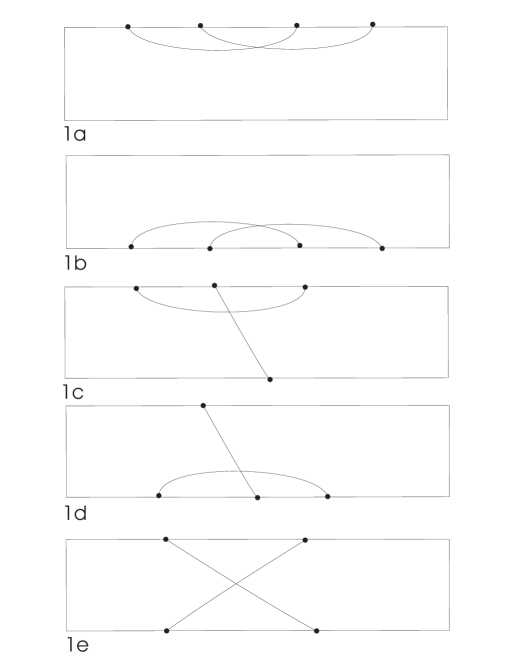
Figure 1:

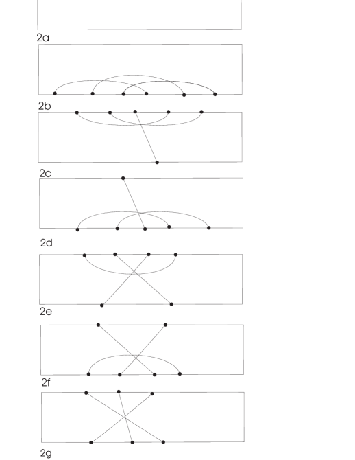
Figure 2:

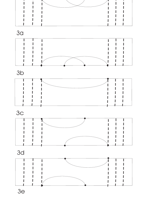
Figure 3:

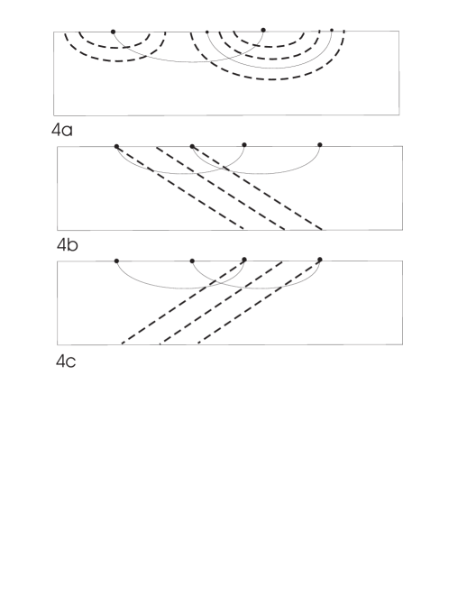
Figure 4:

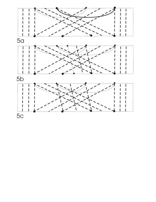
Figure 5:

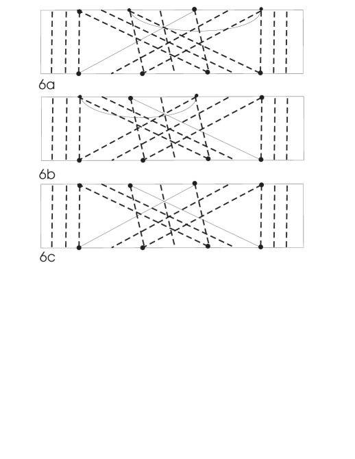
Figure 6:

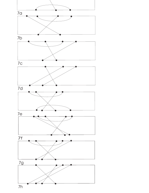
Figure 7:

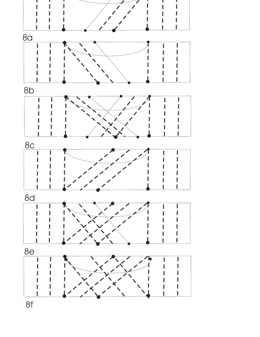
Figure 8:

Figure 9:

References

- [1] M.R. Douglas and N.A. Nekrasov, Noncommutative field theory, Rev. Mod. Phys. 73 (2002) 977 [hep-th/0106048].
- [2] R.J. Szabo, Quantum field theory on noncommutative spaces, Phys. Rept. 378 (2003) 207 [hep-th/0109162].
- [3] A. Bassetto, G. Nardelli and A. Torrielli, Perturbative Wilson loop in two-dimensional noncommutative Yang-Mills theory, Nucl. Phys. B617 (2001) 308 [hep-th/0107147].
- [4] L. Griguolo, D. Seminara and P. Valtancoli, Towards the solution of noncommutative : Morita equivalence and large limit, JHEP 0112 (2001) 024 [hep-th/0110293].
- [5] W. Bietenholz, F. Hofheinz and J. Nishimura, A non-perturbative study of gauge theory on a non-commutative plane, JHEP 0209 (2002) 009 [hep-th/0203151].
- [6] L.D. Paniak and R.J. Szabo, Instanton expansion of noncommutative gauge theory in two dimensions, Commun. Math. Phys. 243 (2003) 343 [hep-th/0203166].
- [7] A. Bassetto, G. Nardelli and A. Torrielli, Scaling properties of the perturbative Wilson loop in two-dimensional noncommutative Yang-Mills theory, Phys. Rev. D66 (2002) 085012 [hep-th/0205210].
- [8] A. Bassetto and F. Vian, Wilson line correlators in two-dimensional noncommutative Yang-Mills theory, JHEP 0210 (2002) 004 [hep-th/0207222].
- [9] L.D. Paniak and R.J. Szabo, Open Wilson lines and group theory of noncommutative Yang–Mills theory in two dimensions, JHEP 0305 (2003) 029 [hep-th/0302162].
- [10] A. Bassetto, G. De Pol and F. Vian, Two-dimensional noncommutative Yang-Mills theory: coherent effects in open Wilson line correlators, JHEP 0306 (2003) 051 [hep-th/0306017].
- [11] E. Langmann, R.J. Szabo and K. Zarembo, Exact solution of quantum field theory on noncommutative phase spaces, JHEP 0401 (2004) 017 [hep-th/0308043].
- [12] H. Dorn and A. Torrielli, Loop equation in two-dimensional noncommutative Yang-Mills theory, JHEP 0401 (2004) 026 [hep-th/0312047].
- [13] W. Bietenholz, F. Hofheinz and J. Nishimura, On the relation between non-commutative field theories at and large N matrix field theories, hep-th/0404179.
- [14] J. Ambjørn, A. Dubin and Y. Makeenko, Wilson loops in 2D noncommutative Euclidean gauge theory: 1. Perturbative expansion, JHEP 0407 (2004) 044 [hep-th/0406187].
- [15] A. Bassetto, G. De Pol, A. Torrielli, and F. Vian, On the invariance under area preserving diffeomorphisms of noncommutative Yang-Mills theory in two dimensions, JHEP 0505 (2005) 061 [hep-th/0503175].
- [16] M. Cirafici, L. Griguolo, D. Seminara, R.J. Szabo, Morita duality and noncommutative Wilson loops in two dimensions, JHEP 0510 (2005) 030 [hep-th/0506016].
- [17] A. Bassetto, G. De Pol, A. Torrielli, and F. Vian, Area preserving diffeomorphisms and Yang-Mills theory in two noncommutative dimensions, Nucl. Phys. Proc. Suppl. 161 (2006) 21 [tt hep-th/0509114].
- [18] J. Volkholz, W. Bietenholz, J. Nishimura, and Y. Susaki, The scaling of QED in a non-commutative space-time, hep-lat/0509146.
- [19] N. Caporaso and S. Pasquetti, Gauge-invariant resummation formalism and unitarity in non-commutative QED, JHEP 0604 (2006) 016 [hep-th/0511127].
- [20] W. Bietenholz, A. Bigarini, F. Hofheinz, J. Nishimura, Y. Susaki, and J. Volkholz, Numerical results for U(1) gauge theory on 2d and 4d non-commutative spaces, Fortsch. Phys. 53 (2005) 418 [hep-th/0501147].
- [21] H. Aoki, J. Nishimura and Y. Susaki, The Index theorem in gauge theory on a discretized 2-D non-commutative torus, hep-th/0602078.
- [22] H. Aoki, J. Nishimura and Y. Susaki, Suppression of topologically nontrivial sectors in gauge theory on 2-D non-commutative geometry, hep-th/0604093.
- [23] M. Riccardi and R.J. Szabo, Wilson loops and area-preserving diffeomorphisms in twisted noncommutative gauge theory, hep-th/0701273.
- [24] T. Filk, Divergences in a field theory on quantum space, Phys. Lett. B376 (1996) 53.
- [25] J. Ambjørn, A. Dubin and Y. Makeenko, Large area asymptote of Wilson loops in 2D noncommutative Euclidean gauge theory, in preparation.
- [26] N. Ishibashi, S. Iso, H. Kawai, and Y. Kitazawa, Wilson loops in noncommutative Yang–Mills, Nucl. Phys. B573 (2000) 573 [hep-th/9910004].
- [27] K. Okuyama, A path integral representation of the map between commutative and noncommutative gauge fields, JHEP 0003 (2000) 016 [hep-th/9910138].
- [28] J. Ambjørn, Y.M. Makeenko, J. Nishimura and R.J. Szabo, Finite- matrix models of noncommutative gauge theory, JHEP 9911 (1999) 029 [hep-th/9911041].
- [29] J. Ambjørn, Y.M. Makeenko, J. Nishimura and R.J. Szabo, Nonperturbative dynamics of noncommutative gauge theory, Phys. Lett. B480 (2000) 399 [hep-th/0002158].
- [30] S.-J. Rey and R. von Unge, S-Duality, noncritical open string and noncommutative gauge theory, Phys. Lett. B499 (2001) 215 [hep-th/0007089].
- [31] S. Das and S.-J. Rey, Open Wilson lines in noncommutative gauge theory and tomography of holographic dual supergravity, Nucl. Phys. B590 (2000) 453 [hep-th/0008042].
- [32] D.J. Gross, A. Hashimoto and N. Itzhaki, Observables of noncommutative gauge theories, Adv. Theor. Math. Phys. 4 (2000) 893 [hep-th/0008075].
- [33] M. Abou-Zeid and H. Dorn, Dynamics of Wilson observables in noncommutative gauge theory, Phys. Lett. B504 (2001) 165 [hep-th/0009231].
- [34] M. Rozali and M. van Raamsdonk, Gauge invariant correlators in noncommutative gauge theory, Nucl. Phys. B608 (2001) 103 [hep-th/0012065].
- [35] A. Dhar and Y. Kitazawa, High-energy behavior of Wilson lines, JHEP 0102 (2001) 004 [hep-th/0012170].
-
[36]
V.A. Kazakov and I.K. Kostov,
Nonlinear strings in two-dimensional theory,
Nucl. Phys. B176 (1980) 199;
N. Bralić, Exact computation of loop averages in two-dimensional Yang–Mills theory, Phys. Rev. D22 (1980) 3090;
V.A. Kazakov, Wilson loop average for an arbitrary contour in two-dimensional gauge theory, Nucl. Phys. B179 (1981) 283. - [37] S. Minwalla, M. van Raamsdonk and N. Seiberg, Noncommutative perturbative dynamics, JHEP 0002 (2000) 020 [hep-th/9912072].
-
[38]
D. Gross,
Two-dimensional QCD as a string theory,
Nucl. Phys. B400 (1993) 161;
D.J. Gross and W.I. Taylor, Two-dimensional QCD is a string theory, Nucl. Phys. B400 (1993) 181; Twists and Wilson loops in the string theory of two-dimensional QCD, Nucl. Phys. B403 (1993) 395.