Noncommutative Induced Gauge Theory

Abstract

We consider an external gauge potential minimally coupled to a renormalisable scalar theory on 4-dimensional Moyal space and compute in position space the one-loop Yang-Mills-type effective theory generated from the integration over the scalar field. We find that the gauge invariant effective action involves, beyond the expected noncommutative version of the pure Yang-Mills action, additional terms that may be interpreted as the gauge theory counterpart of the harmonic oscillator term, which for the noncommutative $\varphi^{4}$-theory on Moyal space ensures renormalisability. The expression of a possible candidate for a renormalisable action for a gauge theory defined on Moyal space is conjectured and discussed.

^aLaboratoire de Physique Théorique, Bât. 210
Université Paris XI, F-91405 Orsay Cedex, France
e-mail: axelmg@melix.net, jean-christophe.wallet@th.u-psud.fr
^bMathematisches Institut der Westfälischen Wilhelms-Universität
Einsteinstraße 62, D-48149 Münster, Germany
e-mail: raimar@math.uni-muenster.de

1 Introduction.

In the past few years, an intense activity has been devoted to the study of various classes of field theories defined on Moyal spaces (see e.g. [1, 2]). These prototypes of noncommutative field theories involve numerous features stemming from noncommutative geometry [3, 4, 5] and are thus interesting in themselves. This interest was further increased by the observation that similar noncommutative field theories seem to emerge rather naturally from limiting regimes of string theory and matrix theory in magnetic backgrounds [6, 7]. See also [8, 9] for connections between noncommutative geometry and string theory. Recall that in noncommutative geometry the commutative algebras of functions defined on differentiable manifolds (roughly speaking the coordinates spaces) are replaced by associative but noncommutative algebras further interpreted as algebras of functions on “noncommutative spaces”. Within this algebraic framework, natural noncommutative analogues of the main geometrical objects usually involved in field theories can be algebraically defined (such as connections, curvatures, vector bundles) so that the construction of various noncommutative analogues of field theories can be undertaken (see e.g. [10]). The starting relevant configuration spaces for the noncommutative field theories are modules over the associative algebras which are naturally viewed as noncommutative analogues for the set of sections of vector bundles. One example of associative algebra among many others is provided by the associative Moyal algebras [11, 12] therefore playing the role of “noncommutative Moyal spaces”.

The simplest generalisations of scalar theories to Moyal space were shown to suffer from the so called UV/IR-mixing [13, 14], a phenomenon that makes the renormalisability very unlikely. Basically, the UV/IR-mixing results from the existence of potentially dangerous non-planar diagrams which, albeit UV finite, become singular at exceptional (low) external momenta. This triggers the occurrence of UV divergences in higher order diagrams in which they are involved as subdiagrams. This signals that UV and IR scales are related in a non-trivial way which should in principle invalidate a Wilson-type renormalisation scheme [15, 16]. An appealing solution to the UV/IR-mixing has been recently proposed by Grosse and Wulkenhaar [17, 18] within the noncommutative $\varphi^{4}$ model on the 4-dimensional Moyal space where $\varphi$ is real-valued. They showed that the UV/IR-mixing can be suppressed by supplementing the initial action with a harmonic oscillator term leading to a renormalisable noncommutative quantum field theory. The initial proof [17] was performed within the matrix-base formalism, roughly speaking a basis for the (Schwarz class) functions for which the associative product of the Moyal algebra is a simple matrix product. This cumbersome proof was simplified through a reformulation into the (position) $x$-space formalism in [19] which exhibits some advantages compared to the matrix-base formulation. For instance, the propagator in $x$-space can be explicitly computed (as a Mehler kernel [20, 21]) and actually used in calculations. Besides, it makes easier the comparison of the renormalisation group for noncommutative theories and their commutative counterpart.

Other renormalisable noncommutative matter field theories on Moyal spaces have been obtained. One is the complex-valued scalar theory studied in [19] which can be viewed as a modified version of the LSZ model [22, 23] (the scalar theory in [24] is super-renormalisable). Note that interesting solvable noncommutative scalar field theories have also been considered in [25, 26, 27]. As far as fermionic theories are concerned, a Moyal space version of the Gross-Neveu model [28] (see also [29, 30]), called the orientable noncommutative Gross-Neveu model, has been recently shown to be renormalisable to all orders [31, 32] (see also [33]). It is worth mentioning that this noncommutative field theory still exhibits some UV/IR-mixing, even in the presence of the fermionic version of the harmonic oscillator quadratic term introduced in [17], which however does not prevent the theory from being renormalisable. Note that in [34] (see also [35]) the large-$N$ limit of the noncommutative Gross-Neveu model, however with a restricted interaction, has been studied; renormalisability is shown at this limit together with asymptotic freedom. One should keep in mind that the fact that the orientable Gross-Neveu model is renormalisable in spite of some remaining UV/IR-mixing [31, 32] indicates that further investigations are needed to actually clarify the role of various generalisations of the above-mentioned harmonic oscillator term, of the related covariance under the Langmann-Szabo duality [36] and of their impact in the control of the UV/IR-mixing and renormalisability.

So far, the construction of a renormalisable gauge theory on noncommutative Moyal spaces remains still unsolved. The naive noncommutative extension of the pure Yang-Mills action on the Moyal space exhibits UV/IR mixing [37, 38] which makes its renormalisability quite unlikely unless it is suitably modified. It can be easily realized that the initial solution proposed in [17] within the real-valued $\varphi^{4}$-model cannot be merely extended to gauge theories on Moyal spaces. In the absence of clear guideline, one reasonable way to follow is to assume that the Langmann-Szabo duality may appear as a necessary ingredient in the construction of a renormalisable gauge theory as it has been the case for the real-valued $\varphi^{4}$-model. Then, any attempt to adapt the solution given in [17] to gauge theories would presumably amount to reconcile within a modified action its invariance under gauge transformations with some covariance under the Langmann-Szabo duality. More technically, one has to determine whether or not the naive noncommutative Yang-Mills action can be supplemented by additional terms that preserve gauge invariance while making possible the appearance of covariance under the Langmann-Szabo duality. A convenient way to actually determine all the above-mentioned additional gauge invariant terms can be achieved by computing, at least at the one-loop order, the noncommutative effective gauge theory stemming from a matter field theory coupled to an external gauge potential in a gauge-invariant way. This is the main purpose of the present paper.

The paper is organised as follows. We start from a renormalisable scalar (Euclidean) field theory extending to complex-valued fields $\phi$ the renormalisable noncommutative $\varphi^{4}$-model with harmonic oscillator term studied in [17, 19]. This is presented in section 2 where we also collect the main technical tools. The above action is minimally coupled to an external gauge potential giving rise to a gauge-invariant action $S(\phi,A)$. The analysis is based consistently on the usual algebraic definition of noncommutative connections for which the modules of the Moyal algebra plays the role of the set of sections of vector bundles of the ordinary geometry, while the noncommutative analogue of gauge transformations are naturally associated with automorphism of (hermitian) modules. This is presented in detail in the second part of section 2. From $S(\phi,A)$, we compute the one-loop effective action $\Gamma(A)$ obtained as usual by formally integrating out the scalar field. The corresponding calculation of the various contributions relevant to the effective action is presented in section 3. All the computations are performed within the $x$-space formalism. The resulting action is further analysed and discussed in section 4. The implications of the non-vanishing of the one-point (tadpole) contribution are outlined. This non-vanishing triggers automatically the occurrence of gauge invariant terms supplementing the noncommutative version of the pure Yang-Mills term in the effective action. This suggests a possible expression of a candidate for a renormalisable action for a gauge theory defined on Moyal spaces in which these additional terms would be the gauge theory counterpart of the the harmonic term ensuring the renormalisability of the $\varphi^{4}$-theory.

2 External gauge potentials coupled to scalar models.

2.1 The 4-dimensional complex scalar model.

We first collect the mathematical tools entering the definition of the Moyal algebra that will be relevant for the ensuing analysis. A more mathematical presentation can be found in [11, 12]. In the following, the “$\star$” symbol denotes the associative Moyal-Groenenwald product. It can be first defined on ${\cal{S}}({\mathbb{R}}^{4})$ (denoted in short by ${\cal{S}}$ in the following), the space of complex-valued Schwartz functions on ${\mathbb{R}}^{4}$ with fast decay at infinity, by

$$(f\star h)(x)={{1}\over{(2\pi)^{4}}}\int d^{4}y\,d^{4}k\ f(x+{{1}\over{2}}\Theta.k)\,h(x+y)e^{ik.y},\quad\forall f,h\in{\cal{S}},$$ (2.1)

such that $(f\star h)\in{\cal{S}}$, where $\Theta.k\equiv\Theta_{\mu\nu}k^{\nu}$. Moreover, $\Theta_{\mu\nu}$ is an invertible constant skew-symmetric matrix which in 4D can be chosen as $\Theta=\theta{{\Sigma}}$ with

$${{\Sigma}}=\begin{pmatrix}J&0\\ 0&J\end{pmatrix},$$ (2.2)

where the $2\times 2$ matrix $J$ is given by $J=\begin{pmatrix}0&-1\\ 1&0\end{pmatrix}$ and the parameter $\theta$ has mass dimension $-2$. Let ${\cal{S}}^{\prime}$ denotes the space of tempered distributions. Then, the $\star$-product is further extended to ${\cal{S}}^{\prime}\times{\cal{S}}$ upon using duality of linear spaces: $\langle T\star f,h\rangle=\langle T,f\star h\rangle$, $\forall T\in{\cal{S}}^{\prime}$, $\forall f,h\in{\cal{S}}$, In a similar way, (2.1) can be extended to ${\cal{S}}\times{\cal{S}}^{\prime}$. Owing to the smoothening properties of (2.1) together with

$$\int d^{4}x\ (f\star h)(x)=\int d^{4}x\ f(x).h(x),$$ (2.3)

where the symbol “.” denotes the (commutative) usual pointwise product, one can show that $T\star f$ and $f\star T$ are smooth functions [11, 12]. Now, let ${\cal{L}}$ (resp. ${\cal{R}}$) denote the subspace of ${\cal{S}}^{\prime}$ whose multiplication from right (resp. left) by any Schwartz functions is a subspace of ${\cal{S}}$, namely

$${\cal{L}}=\big{\{}T\in{\cal{S}}^{\prime}\leavevmode\nobreak\ :\leavevmode\nobreak\ \leavevmode\nobreak\ T\star f\in{\cal{S}},\leavevmode\nobreak\ \forall f\in{\cal{S}}\big{\}},\quad{\cal{R}}=\big{\{}T\in{\cal{S}}^{\prime}\leavevmode\nobreak\ :\leavevmode\nobreak\ \leavevmode\nobreak\ f\star T\in{\cal{S}},\leavevmode\nobreak\ \forall f\in{\cal{S}}\big{\}}.$$ (2.4)

The Moyal algebra, hereafter denoted by ${\cal{M}}$, is then defined as

$${\cal{M}}={\cal{L}}\cap{\cal{R}}.$$ (2.5)

The Moyal algebra is a unital algebra which involves, in particular, the “coordinate” functions $x_{\mu}$ satisfying $[x_{\mu},x_{\nu}]_{\star}=i\Theta_{\mu\nu}$, where this last relation is well defined on ${\cal{M}}$ ($[a,b]_{\star}\equiv a\star b-b\star a$). Other relevant properties of the $\star$-product that hold on ${\cal{M}}$ are

$$\partial_{\mu}(f\star h)=\partial_{\mu}f\star h+f\star\partial_{\mu}h,\qquad(f\star h)^{\dagger}=h^{\dagger}\star f^{\dagger},\qquad[x_{\mu},f]_{\star}=i\Theta_{\mu\nu}\partial_{\nu}f,$$ (2.6a)

$$x_{\mu}\star f=(x_{\mu}.f)+{{i}\over{2}}\Theta_{\mu\nu}\partial_{\nu}f,\qquad x_{\mu}(f\star h)=(x_{\mu}.f)\star h-{{i}\over{2}}\Theta_{\mu\nu}f\star\partial_{\nu}h,$$ (2.6b)

for any $f,h\in{\cal{M}}$, where in (2.6a) the symbol ^† denotes the complex conjugation that permits one to turn ${\cal{M}}$ into an involutive algebra.

The action for the (Euclidean) scalar model defined on ${\cal{M}}$ that will be considered in this paper is given by

$$S(\phi)=\int d^{4}x\big{(}\partial_{\mu}\phi^{\dagger}\star\partial_{\mu}\phi+\Omega^{2}(\widetilde{x}_{\mu}\phi)^{\dagger}\star(\widetilde{x}_{\mu}\phi)+m^{2}\phi^{\dagger}\star\phi\big{)}(x)+S_{int},$$ (2.7)

where $\phi$ is a complex scalar field with mass $m$, $S_{int}$ denotes the interaction terms to be discussed below and we have set ${\widetilde{x}}_{\mu}=2\Theta^{-1}x$. The parameters $\Omega$ and $\lambda$ are dimensionless. At this point, some comments are in order. This model cannot be viewed as related to some LSZ-type model [22, 23] since in that latter case the corresponding action would have been of the form

$$S_{LSZ}(\phi)=\int d^{4}x\big{(}(\partial_{\mu}\phi+i\Omega{\widetilde{x}}_{\mu}\phi)^{\dagger}\star(\partial_{\mu}\phi+i\Omega{\widetilde{x}}_{\mu}\phi)+m^{2}\phi^{\dagger}\star\phi\big{)}(x)+S_{int}.$$ (2.8)

It can easily be realised that the quadratic terms in (2.8) do not coincide with those involved in (2.7), giving rise therefore to different propagators for these actions (as well as, anticipating with the discussion of the next subsection, different minimal coupling prescriptions). Notice however that both actions are covariant under the Langmann-Szabo duality [36]. It turns out, as it will be shown in a while, that the operator $\partial_{\mu}+i\Omega{\widetilde{x}}_{\mu}$ can actually be related to a connection $\nabla^{\zeta}_{\mu}$ with $\zeta=-{{\Omega}\over{1+\Omega}}{\widetilde{x}}_{\mu}$. In (2.7), the term involving $\Omega$ can be viewed as the (complex-valued) scalar counterpart of the harmonic oscillator term first introduced in [17] leading to the construction of a renormalisable noncommutative (real-valued) $\varphi^{4}_{4}$-model.

Although our one-loop computation of effective actions will not depend on the explicit form of the interaction, it is instructive to discuss it more closely in view of the corresponding consequences on the renormalisability of the models. The most general interaction can be written as

$$S_{int}=S_{int}^{0}+S_{int}^{NO}=\int\lambda(\phi^{\dagger}\star\phi\star\phi^{\dagger}\star\phi)(x)+\kappa(\phi^{\dagger}\star\phi^{\dagger}\star\phi\star\phi)(x).$$ (2.9)

We point out that the only diagrams that can be orientated are those occurring in the loopwise expansion obtained from $S_{int}^{O}$ while $S_{int}^{NO}$ yields diagrams in the loopwise expansion that cannot be oriented. Recall now that the proof of the renormalisability of the noncommutative version of the Gross-Neveu model studied in [31] (whose interaction term is the fermionic counterpart of $S_{int}^{O}$) relies heavily on the orientability of the diagrams. It turns out [19] that (2.7) restricted to $S_{int}^{O}$ is renormalisable for any value of $\Omega$. Besides, a similar conclusion applies for the LSZ-type model (2.8) restricted to $S_{int}^{O}$. The proof, as sketched in [19], is somehow similar to the one given in [31] for the noncommutative Gross-Neveu model. At the present time, the actual impact of interaction terms as given by $S_{int}^{NO}$ on the renormalisability of the above models is not known.

The Feynman graphs can be computed from the propagator and interaction vertex derived from (2.7). In the following, we will work within the $x$-space formalism [19] which proves particularly convenient as it simplifies the calculations. The scalar propagator $C(x,y)\equiv\langle\phi(x)\phi^{\dagger}(y)\rangle$ in $x$-space obtained by solving $(\Delta_{x}+{\widetilde{\Omega}}^{2}x^{2}+m^{2})C(x,y)=\delta(x-y)$ is given by

$$C(x,y)={{\Omega^{2}}\over{\pi^{2}\theta^{2}}}\int_{0}^{\infty}\!\!{{dt}\over{\sinh^{2}(2{\widetilde{\Omega}}t)}}\exp\Big{(}-{{{\widetilde{\Omega}}}\over{4}}\coth({\widetilde{\Omega}}t)(x{-}y)^{2}-{{{\widetilde{\Omega}}}\over{4}}\tanh({\widetilde{\Omega}}t)(x{+}y)^{2}-m^{2}t\Big{)},$$ (2.10)

where we have defined ${\widetilde{\Omega}}\equiv 2{{\Omega}\over{\theta}}$. The interaction vertices can be read off from the RHS of

$$\int d^{4}x(\phi^{\dagger}\star\phi\star\phi^{\dagger}\star\phi)(x) =\frac{1}{\pi^{4}\theta^{4}}\int\prod_{i=1}^{4}d^{4}x_{i}\,\phi^{\dagger}(x_{1})\phi(x_{2})\phi^{\dagger}(x_{3})\phi(x_{4})$$ (2.11a)

$$\times\delta(x_{1}-x_{2}+x_{3}-x_{4})e^{-i\sum_{i<j}(-1)^{i+j+1}x_{i}\wedge x_{j}}.$$

We will denote the vertex kernel as

$$V(x_{1},x_{2},x_{3},x_{4}) =\delta(x_{1}-x_{2}+x_{3}-x_{4})e^{-i\sum_{i<j}(-1)^{i+j+1}x_{i}\wedge x_{j}}$$ (2.11b)

in which $x\wedge y\equiv 2x_{\mu}\Theta^{-1}_{\mu\nu}y_{\nu}$. The generic graphical representation of the vertex is depicted on the figure 1. The non-locality of the interaction is conveniently represented by the rhombus appearing on fig. 1 whose vertices correspond to the $x_{i}$’s occurring in (2.11). It is useful to represent the alternate signs in the delta function of (2.11) by plus- and minus-signs, as depicted on the figure. By convention, a plus-sign (resp. minus-sign) corresponds to an incoming field $\phi^{\dagger}$ (resp. outgoing field $\phi$). This permits one to define an orientation on the diagrams obtained from the loop expansion.

Figure 1: Graphical representation for the vertex in the $x$-space, obtained from (2.11). The plus-sign (resp. minus-sign) appearing in the rhombus corresponds to incoming (resp. outgoing) external line associated with ${\phi^{\dagger}}$ (resp. $\phi$).

2.2 Gauge connexions on Moyal Space.

It is necessary to define clearly the mathematical status [4, 5] (see also [39, 10]) of the various objects that will be involved in the minimal coupling prescription. Recall that ${\cal{M}}$ is a unital involutive algebra. Let ${\cal{H}}$ be a right ${\cal{M}}$-module with hermitian structure $h$, that is, a sesquilinear map $h:{\cal{H}}\times{\cal{H}}\to{\cal{M}}$ such that $h(m_{1}\star f_{1},m_{2}\star f_{2})=f_{1}^{\dagger}\star h(m_{1},m_{2})\star f_{2}$, for any $f_{1},f_{2}\in{\cal{M}}$, and $m_{1},m_{2}\in{\cal{H}}$. The algebra ${\cal{M}}$ is assumed to be endowed with a differential calculus based on the derivations $\partial_{\mu}$. The usual concept of connections defined on vector bundles in ordinary geometry can be consistently generalised in noncommutative geometry to connections on projective modules (over an associative algebra). Namely, a connection can be defined (algebraically) by a linear map $\nabla_{\mu}:{\cal{H}}\to{\cal{H}}$ verifying the Leibnitz rule:

$$\nabla_{\mu}(m\star f)=\nabla_{\mu}(m)\star f+m\star\partial_{\mu}f,\ \forall m\in{\cal{H}},\quad\forall f\in{\cal{M}}$$ (2.12)

and preserving the hermitian structure, that is

$$\partial_{\mu}h(m_{1},m_{2})=h(\nabla_{\mu}m_{1},m_{2})+h(m_{1},\nabla_{\mu}m_{2}),\quad\forall m_{1},m_{2}\in{\mathcal{H}}.$$ (2.13)

When ${\cal{H}}={\cal{M}}$, that we assume from now on, it follows from (2.12) that the connection is entirely determined by its action $\nabla_{\mu}(\mathbb{I})$ on the unit $\mathbb{I}\in\mathcal{M}$, denoted by

$$\nabla_{\mu}^{A}(\mathbb{I})\equiv-iA_{\mu},$$ (2.14)

since one has obviously $\nabla^{A}_{\mu}(\mathbb{I}\star f)=\nabla^{A}_{\mu}(\mathbb{I})\star f+\partial_{\mu}f\equiv\partial_{\mu}f-iA_{\mu}\star f$. This therefore represents the gauge potential $A_{\mu}$ in ${\cal{M}}$. Observe that for ${\cal{H}}={\cal{M}}$, a hermitian structure is provided by $h(f_{1},f_{2})=f_{1}^{\dagger}\star f_{2}$, ensuring that the above connections are hermitian.

Gauge transformations hereafter denoted by $\gamma$ are determined by automorphisms of the module ${\cal{M}}$ (keeping in mind that ${\cal{M}}={\cal{H}}$ is considered as a hermitian module over itself) preserving the hermitian structure $h$, $\gamma\in Aut_{h}({\cal{M}})$. One has

$$\gamma(f) =\gamma(\mathbb{I}\star f)=\gamma(\mathbb{I})\star f\ ,\quad\forall f\in{\mathcal{M}},$$

$$h\big{(}\gamma(f_{1}),\gamma(f_{2})\big{)} =h(f_{1},f_{2})\quad\forall f_{1},f_{2}\in\mathcal{M}\qquad\Rightarrow\quad\gamma(\mathbb{I})^{\dagger}\star\gamma(\mathbb{I})=\mathbb{I},$$ (2.15)

so that gauge transformations are entirely determined by $\gamma(\mathbb{I})\in{\cal{U}}(\cal{M})$, where ${\cal{U}}(\cal{M})$ is the group of unitary elements of $\cal{M}$. From now on, we set $\gamma(\mathbb{I})\equiv g$. Then, according to (2.15), the action of the gauge group on any matter field $\phi\in{\cal{M}}$ can be defined by

$$\phi^{g}=g\star\phi$$ (2.16)

for any $g\in{\cal{U}}(\cal{M})$, which may be viewed, in more physical words, as the noncommutative analogue of the transformation of the matter fields under the “fundamental representation of the gauge group”. Note that one has $g^{\dagger}\star g=g\star g^{\dagger}=\mathbb{I}$.

The action of ${\cal{U}}({\cal{M}})$ on the connection $\nabla^{A}_{\mu}$ is given by

$$(\nabla^{A}_{\mu})^{\gamma}(\phi)=\gamma(\nabla^{A}_{\mu}(\gamma^{-1}\phi)),\quad\forall\phi\in{\cal{M}}.$$ (2.17)

By further using $\gamma(\phi)=\gamma(\mathbb{I}\star\phi)=g\star\phi$ together with the expression of the covariant derivative

$$\nabla_{\mu}^{A}(\phi)=\partial_{\mu}\phi-iA_{\mu}\star\phi$$ (2.18)

and the fact that $(\nabla_{\mu}^{A})^{g}\equiv\partial_{\mu}-iA^{g}_{\mu}$, one obtains the following gauge transformation for the gauge potential $A_{\mu}$

$$A_{\mu}^{g}=g\star A_{\mu}\star g^{\dagger}+ig\star\partial_{\mu}g^{\dagger}.$$ (2.19)

In the present noncommutative (algebraic) framework, the space of gauge potentials $A_{\mu}\in\cal{M}$ is a linear space (this comes basically from the fact that ${\cal{M}}$, as a module, is a linear space). Note that any one-form can be used to define a connection so that if some $A_{\mu}$ defines a connection, then $\lambda A_{\mu}$, $\forall\lambda\in{\mathbb{R}}$, defines another connection. There is a subtlety here that must be pointed out. The gauge transformations do not preserve the structure of linear space of gauge potentials since

$$(\lambda A_{\mu})^{g}-\lambda(A_{\mu}^{g})=i(1-\lambda)g\star\partial_{\mu}g^{{\dagger}}.$$ (2.20)

This is easily obtained by comparing how the gauge transformations as given by (2.17) operate on $\nabla_{\mu}^{\lambda A}$ and $\nabla_{\mu}^{A}$ according to (2.18) and expresses the fact that multiplication of a gauge potential by a scalar and gauge transformation are two noncommuting operations. The same discussion applies to the sum of two gauge potentials $A_{1}+A_{2}$.

It is useful to exhibit a special reference connection that will play a salient role in the following. It turns out that

$$\xi_{\mu}\equiv-{{1}\over{2}}\widetilde{x}_{\mu}$$ (2.21)

defines a connection invariant under gauge transformations. Note that the occurrence of gauge-invariant connections is not new in noncommutative geometry and has been already mentioned in earlier studies focused in particular on matrix-valued field theories [39, 40, 41, 42]. Indeed, according to (2.18), the connection $\nabla_{\mu}^{\xi}$ associated to $\xi_{\mu}$ verifies

$$\nabla^{\xi}_{\mu}\phi=\partial_{\mu}\phi-i\xi_{\mu}\star\phi=-i\phi\star\xi_{\mu},$$ (2.22)

where the second equality stems from the following relation

$$\partial_{\mu}\phi=[i\xi_{\mu},\phi]_{\star}$$ (2.23)

which simply expresses the fact that the derivative $\partial_{\mu}$ in $\cal{M}$ is an inner derivative. Then, as $\nabla_{\mu}^{\xi}$ given by right multiplication commutes with the gauge transformation (2.17) given by left multiplication, it is easy to realise that

$$(\nabla_{\mu}^{\xi})^{g}(\phi)=g\star(\nabla_{\mu}^{\xi}(g^{\dagger}\star\phi))=-i\phi\star\xi_{\mu}=\nabla_{\mu}^{\xi}\phi.$$ (2.24)

The second equality stems from (2.22), which shows that the connection $\nabla_{\mu}^{\xi}$ is invariant under the gauge transformations, from which follows that

$$\xi_{\mu}^{g}=\xi_{\mu},$$ (2.25)

as it could have been checked directly by combining the actual expression for $\xi_{\mu}$ with (2.19) and (2.23). In the present Moyal framework, the existence of the above invariant connection seems to be an unavoidable consequence of the existence of inner derivations as defined by (2.23) (it turns out that all derivations on the Moyal algebra are inner derivations).

Let us introduce now

$$\nabla^{A}_{\mu}-\nabla^{\xi}_{\mu}=-i(A_{\mu}-\xi_{\mu})\equiv-i\mathcal{A}_{\mu}$$ (2.26)

which, as the difference of two connections, defines obviously a tensorial form ${\cal{A}}_{\mu}$ whose gauge transformations are given by

$$\mathcal{A}_{\mu}^{g}=g\star\mathcal{A}_{\mu}\star g^{\dagger}.$$ (2.27)

This tensorial form has been sometimes called in the String Theory literature the covariant coordinates (see e.g. [1] and references therein). Given a connection $\nabla_{\mu}^{A}$ (or equivalently a gauge potential $A_{\mu}$), the corresponding curvature is given by

$$F_{\mu\nu}^{A}=i[\nabla^{A}_{\mu},\nabla^{A}_{\nu}]_{\star}=\partial_{\mu}A_{\nu}-\partial_{\nu}A_{\mu}-i[A_{\mu},A_{\nu}]_{\star},$$ (2.28)

with gauge transformations taking the usual form

$$(F_{\mu\nu}^{A})^{g}=g\star F_{\mu\nu}^{A}\star g^{\dagger}.$$ (2.29)

By further combining (2.28) with (2.23) and (2.26), the curvature can be reexpressed as

$$F_{\mu\nu}^{A}=\Theta_{\mu\nu}^{-1}-i[\mathcal{A}_{\mu},\mathcal{A}_{\nu}]_{\star}.$$ (2.30)

Note that the invariant connection defined by $\xi_{\mu}$ is a constant curvature connection since $F_{\mu\nu}^{\xi}=\Theta_{\mu\nu}^{-1}$.

Another type of transformations given by $\phi^{U}=U\star\phi\star U^{\dagger}$, which may be viewed as the noncommutative analogue of transformations of matter fields in the adjoint representation, has been also considered in the literature. These transformations will be more closely analysed in the next subsection.

2.3 The minimal coupling prescription.

Let us assume that the action of the gauge group on the matter fields $\phi$ is given by (2.16). Then, owing to the special role played by the coordinate functions $x_{\mu}$ through the invariant “gauge potential” (2.21) involved in $\nabla^{\xi}_{\mu}$ and the expression for the inner derivatives (2.23), it follows that a natural choice for the minimal coupling of the action (2.7) to an external gauge field $A_{\mu}$ is obtained by performing the usual substitution

$$\partial_{\mu}\to\nabla_{\mu}^{A}$$ (2.31)

on the action (2.7) provided this latter is reexpressed in terms of $\partial_{\mu}$ and $\nabla_{\mu}^{\xi}$, using in particular the following identity:

$$\widetilde{x}_{\mu}\phi=\widetilde{x}_{\mu}\star\phi-i\partial_{\mu}\phi=-i(\partial_{\mu}\phi-2i\xi_{\mu}\star\phi)=-2i\nabla_{\mu}^{\xi}\phi+i\partial_{\mu}\phi.$$ (2.32)

By using (2.32), one easily infers that the minimal coupling prescription can be conveniently written as

$$\partial_{\mu}\phi \mapsto\nabla_{\mu}^{A}\phi=\partial_{\mu}\phi-iA_{\mu}\star\phi,$$ (2.33)

$$\widetilde{x}_{\mu}\phi \mapsto-2i\nabla_{\mu}^{\xi}\phi+i\nabla_{\mu}^{A}\phi=\widetilde{x}_{\mu}\phi+A_{\mu}\star\phi.$$ (2.34)

Note that gauge invariance of the resulting action functional is obviously obtained thanks to the relation $(\nabla^{A,\xi}_{\mu}(\phi))^{g}=g\star(\nabla^{A,\xi}_{\mu}(\phi))$.

By applying the above minimal coupling prescription to (2.7), we obtain the following gauge-invariant action

$$S(\phi,A)= S(\phi)+\int d^{4}x\ \big{(}(1+\Omega^{2})\phi^{\dagger}\star(\widetilde{x}_{\mu}A_{\mu})\star\phi$$

$$-(1-\Omega^{2})\phi^{\dagger}\star A_{\mu}\star\phi\star\widetilde{x}_{\mu}+(1+\Omega^{2})\phi^{\dagger}\star A_{\mu}\star A_{\mu}\star\phi\big{)}(x),$$ (2.35)

where $S(\phi)$ is given by (2.7) with $S_{int}$ restricted to its gauge-invariant part $S_{int}^{O}$, see (2.9). At this level, it is instructive to interpret the action (2.8) in the light of the algebraic framework that has been developed above. As already mentioned in subsection 2.1, the operator $\partial_{\mu}+i\Omega{\widetilde{x}}_{\mu}$ is actually related to a connection $\nabla^{\zeta}_{\mu}$ with

$$\zeta_{\mu}=\frac{2\Omega}{1+\Omega}\xi_{\mu},$$ (2.36)

since the following relation

$$(\partial_{\mu}+i\Omega{\widetilde{x}}_{\mu})\phi=(1+\Omega)\Big{(}\partial_{\mu}\phi-i{{2\Omega}\over{1+\Omega}}\xi_{\mu}\star\phi\Big{)}=(1+\Omega)\nabla^{\zeta}_{\mu}(\phi)$$ (2.37)

holds in view of (2.18). The action (2.8) can then be rewritten as

$$S_{LSZ}(\phi)=\int d^{4}x\big{(}(1+\Omega)^{2}(\nabla^{\zeta}_{\mu}(\phi))^{\dagger}\star\nabla^{\zeta}_{\mu}(\phi)+m^{2}\phi^{\dagger}\star\phi\big{)}(x)+S_{int},$$ (2.38)

where $\zeta$ is given by (2.36) which, for $\Omega\neq 0$, makes explicit the invariance of the action under the gauge transformations $\phi^{g}=g\star\phi$ for any $g\in{\cal{U}}({\cal{M}})$. Notice that a similar comment applies to the noncommutative version of the (two-dimensional) Gross-Neveu model considered recently in [31]. It can be easily realised that the corresponding action quoted in [31] can be cast into the form

$$S_{GN}=\int d^{2}x\big{(}-i(1+\Omega){\bar{\psi}}\gamma^{\mu}\nabla_{\mu}^{\zeta}\psi+m{\bar{\psi}}\psi\big{)}(x)+...,$$ (2.39)

where the ellipses denote interaction terms, $\psi$ is a spinor and the antihermitian $\gamma$ matrices satisfy $\{\gamma_{\mu},\gamma_{\nu}\}=-2\delta_{\mu\nu}$. In physical words, it should be clear that these two latter actions can be interpreted as matter actions already coupled to an external (background) gauge potential $\zeta_{\mu}$ (while the action (2.7) does not obviously support this interpretation).

As announced in the last subsection, another type of transformations given by

$$\phi^{U}=U\star\phi\star U^{\dagger}\equiv\alpha(\phi),$$ (2.40)

for any $U\in{\cal{U}}({\cal{M}})$, has been also considered in the literature. It is instructive to confront the actual mathematical status of these transformations to the algebraic framework developed in subsection 2.2. In fact, it should be clear that (2.40) defines an automorphism $\alpha$ of algebra,

$$\alpha(\phi_{1}\star\phi_{2})=\alpha(\phi_{1})\star\alpha(\phi_{2}),$$ (2.41)

but not an automorphism of the module (which would satisfy $\alpha(\phi_{1}\star\phi_{2})=\alpha(\phi_{1})\star\phi_{2}$) except when $U$ is in the centre of ${\cal{M}}$ (which in the present case is equal to ${\mathbb{C}}$). Actually, the noncommutative analogue of the adjoint representation of the gauge group is constructed with the help of the real structure $J$ (see e.g. [5]). This requires to replace the algebra $\mathcal{M}$ by $\mathcal{M}\otimes\mathcal{M}^{o}$, where $\mathcal{M}^{o}$ is the opposite algebra. The only minimal coupling prescription which is compatible with modules over the algebra $\mathcal{M}$ is given by (2.33), (2.34).

Nonetheless, in order to prepare the discussion of section 4, we simply quote the action

$$S_{adj}(\phi,A)= S(\phi)+\int d^{4}x\ \big{(}(1+\Omega^{2})(\phi^{\dagger}\star(\widetilde{x}_{\mu}A_{\mu})\star\phi+\phi\star(\widetilde{x}_{\mu}A_{\mu})\star\phi^{\dagger})$$

$$-(1-\Omega^{2})(\phi^{\dagger}\star A_{\mu}\star\phi\star\widetilde{x}_{\mu}+\phi\star A_{\mu}\star\phi^{\dagger}\star\widetilde{x}_{\mu})-2(1-\Omega^{2})\phi^{\dagger}\star A_{\mu}\star\phi\star A_{\mu}$$

$$+(1+\Omega^{2})(\phi^{\dagger}\star A_{\mu}\star A_{\mu}\star\phi+\phi\star A_{\mu}\star A_{\mu}\star\phi^{\dagger})\big{)}(x),$$ (2.42)

which is invariant under the adjoint gauge transformation (2.40). This is obtained from (2.7) by the substitution

$$\partial_{\mu}\phi\mapsto\partial_{\mu}\phi-i[A_{\mu},\phi]_{\star}\,,\qquad\widetilde{x}_{\mu}\phi\mapsto\widetilde{x}_{\mu}\phi+\{A_{\mu},\phi\}_{\star}\,.$$ (2.43)

3 The one-loop effective action.

In this section we will calculate the one-loop effective action starting from the action $S(\phi,A)$ (2.35). Recall that the effective action is formally obtained from

$$e^{-\Gamma(A)}\equiv\int D\phi D\phi^{\dagger}e^{-S(\phi,A)}=\int D\phi D\phi^{\dagger}e^{-S(\phi)}e^{-S_{int}(\phi,A)},$$ (3.1)

where $S(\phi)$ is given by (2.7) and $S_{int}(\phi,A)$ can be read off from (2.35) and (2.7). At the one-loop order, (3.1) reduces to

$$e^{-\Gamma_{1loop}(A)}=\int D\phi D\phi^{\dagger}e^{-S_{free}(\phi)}e^{-S_{int}(\phi,A)},$$ (3.2)

where $S_{free}(\phi)$ is simply the quadratic part of (2.7). The corresponding diagrams are depicted on the figures 3-6.

The additional vertices involving $A_{\mu}$ and/or $\xi_{\mu}$ and generated by the minimal coupling can be obtained by combining (2.11) with (2.35) and the generic relation

$$\int d^{4}x(f_{1}\star f_{2}\star f_{3}\star f_{4})(x)=\frac{1}{\pi^{4}\theta^{4}}\int\prod_{i=1}^{4}d^{4}x_{i}\,f_{1}(x_{1})f_{2}(x_{2})f_{3}(x_{3})f_{4}(x_{4})$$

$$\times\delta(x_{1}-x_{2}+x_{3}-x_{4})e^{-i\sum_{i<j}(-1)^{i+j+1}x_{i}\wedge x_{j}}.$$ (3.3)

These vertices are depicted on the figure 2. Note that additional overall factors must be taken into account. These are indicated on the figure 2.

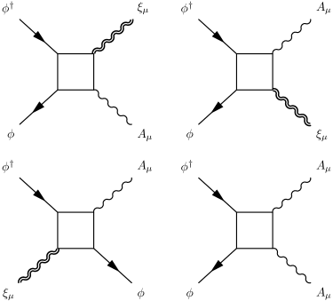
Figure 2: Graphical representation for the vertices carrying the external gauge potential $A_{\mu}$ involved in the action (2.35). The overall factor affecting the two uppermost vertices is $(1+\Omega^{2})$. From left to right, the overall factors affecting the lower vertices are respectively equal to $-2(1-\Omega^{2})$ and $-(1+\Omega^{2})$.

3.1 The tadpole for the scalar model.

Figure 3: The non vanishing tadpole diagram. To simplify the figure, we do not explicitly draw all the diagrams that would be obtained from the vertices given on the figure 2 but indicate only the overall topology of the corresponding diagrams. Notice that the background lines are not explicitly depicted.

Using the expression for the vertices and the minimal coupling, the amplitude corresponding to the tadpole on figure 3 is

$$\mathcal{T}_{1}=\frac{1}{\pi^{4}\theta^{4}}\int d^{4}x\ d^{4}u\ d^{4}z\ A_{\mu}(u)\ e^{-i(u-x)\wedge z}\ C(x+z,x)\ ((1-\Omega^{2})(2\widetilde{x}_{\mu}+\widetilde{z}_{\mu})-2\widetilde{u}_{\mu}).$$ (3.4)

Combining this with the explicit expression for the propagator (2.10), (3.4) can be expressed as

$$\mathcal{T}_{1}= \frac{\Omega^{2}}{4\pi^{6}\theta^{6}}\int d^{4}x\ d^{4}u\ d^{4}z\int_{0}^{\infty}\frac{dt\ e^{-tm^{2}}}{\sinh^{2}(\widetilde{\Omega}t)\cosh^{2}(\widetilde{\Omega}t)}\ A_{\mu}(u)\ e^{-i(u-x)\wedge z}$$

$$\times e^{-\frac{\widetilde{\Omega}}{4}(\coth(\widetilde{\Omega}t)z^{2}+\tanh(\widetilde{\Omega}t)(2x+z)^{2}}((1-\Omega^{2})(2\widetilde{x}_{\mu}+\widetilde{z}_{\mu})-2\widetilde{u}_{\mu}).$$ (3.5)

At this point, we find convenient to introduce the following 8-dimensional vectors $X$, $J$ and the $8\times 8$ matrix $K$ defined by

$$X=\begin{pmatrix}x\\ z\end{pmatrix},\quad K=\begin{pmatrix}4\tanh(\widetilde{\Omega}t)\mathbb{I}&2\tanh(\widetilde{\Omega}t)\mathbb{I}-2i\Theta^{-1}\\ 2\tanh(\widetilde{\Omega}t)\mathbb{I}+2i\Theta^{-1}&(\tanh(\widetilde{\Omega}t)+\coth(\widetilde{\Omega}t))\mathbb{I}\end{pmatrix},\quad\ J=\begin{pmatrix}0\\ i\tilde{u}\end{pmatrix}.$$ (3.6)

This permits one to reexpress (3.5) in a form such that some Gaussian integrals can be easily performed. Note that this latter procedure can be adapted to the calculation of the higher order Green functions (see subsection 3.2). The combination of (3.6) with (3.5) then yields

$$\mathcal{T}_{1}= \frac{\Omega^{2}}{4\pi^{6}\theta^{6}}\int d^{4}x\ d^{4}u\ d^{4}z\int_{0}^{\infty}\frac{dt\ e^{-tm^{2}}}{\sinh^{2}(\widetilde{\Omega}t)\cosh^{2}(\widetilde{\Omega}t)}\ A_{\mu}(u)$$

$$\times e^{-\frac{1}{2}X.K.X+J.X}((1-\Omega^{2})(2\widetilde{x}_{\mu}+\widetilde{z}_{\mu})-2\widetilde{u}_{\mu}).$$ (3.7)

By performing the Gaussian integrals on $X$, we find

$$\mathcal{T}_{1}=-\frac{\Omega^{4}}{\pi^{2}\theta^{2}(1+\Omega^{2})^{3}}\int d^{4}u\int_{0}^{\infty}\frac{dt\ e^{-tm^{2}}}{\sinh^{2}(\widetilde{\Omega}t)\cosh^{2}(\widetilde{\Omega}t)}\ A_{\mu}(u)\widetilde{u}_{\mu}\ e^{-\frac{2\Omega}{\theta(1+\Omega^{2})}\tanh(\widetilde{\Omega}t)u^{2}}.$$ (3.8)

Then, inspection of the behaviour of (3.8) for $t\to 0$ shows that this latter expression has a quadratic as well as a logarithmic UV divergence. Indeed, by performing a Taylor expansion of (3.8), one obtains

$$\mathcal{T}_{1}= -\frac{\Omega^{2}}{4\pi^{2}(1+\Omega^{2})^{3}}\left(\int d^{4}u\ \widetilde{u}_{\mu}A_{\mu}(u)\right)\ \frac{1}{\epsilon}\ -\frac{m^{2}\Omega^{2}}{4\pi^{2}(1+\Omega^{2})^{3}}\left(\int d^{4}u\ \widetilde{u}_{\mu}A_{\mu}(u)\right)\ \ln(\epsilon)$$

$$-\frac{\Omega^{4}}{\pi^{2}\theta^{2}(1+\Omega^{2})^{4}}\left(\int d^{4}u\ u^{2}\widetilde{u}_{\mu}A_{\mu}(u)\right)\ \ln(\epsilon)\ +\dots,$$ (3.9)

where $\epsilon\to 0$ is a cut-off and the ellipses denote finite contributions. The fact that the tadpole is (a priori) non-vanishing is a rather unusual feature for a Yang-Mills type theory. This will be discussed more closely in section 4.

3.2 The multi-point contributions.

The 2, 3 and 4-point functions can be computed in a way similar to the one used for the tadpole. The algebraic manipulations are standard but cumbersome so that we only give below the final expressions for the various contributions.

Figure 4: Relevant one-loop diagrams contributing to the two-point function. To simplify the figure, we do not explicitly draw all the diagrams that would be obtained from the vertices given in figure 2 but indicate only the overall topology of the corresponding diagrams. Notice that the background lines are not explicitly depicted. The leftmost (resp. rightmost) diagram corresponds to the contribution $\mathcal{T}_{2}^{\prime}$ (resp. $\mathcal{T}_{2}^{\prime\prime}$).

Let us start with the two-point function. The regularisation of the diverging amplitudes is performed in a way that preserves gauge invariance of the most diverging terms (which in four dimensions are UV quadratically diverging) so that the cut-off $\epsilon$ to be put on the various integrals over the Schwinger parameters, says $\int_{\epsilon}^{\infty}dt$, must be suitably chosen. In the present case, we find that this can be achieved with $\int_{\epsilon}^{\infty}dt$ for $\mathcal{T}_{2}^{\prime\prime}$ while for $\mathcal{T}_{2}^{\prime}$ the regularisation must be performed with $\int_{\epsilon/4}^{\infty}$. Such an adaptation by hand of the scheme is not surprising. The one-loop effective action can be expressed in terms of heat kernels [43],

$$\Gamma_{1loop}(\phi,A) =-\frac{1}{2}\int_{0}^{\infty}\frac{dt}{t}\,\mathrm{Tr}\big{(}e^{-tH(\phi,A)}-e^{-tH(0,0)}\big{)}$$ (3.10)

$$=-\frac{1}{2}\lim_{s\to 0}\Gamma(s)\,\mathrm{Tr}\big{(}H^{-s}(\phi,A)-H^{-s}(0,0)\big{)},$$

where $H(\phi,A)=\frac{\delta^{2}S(\phi,A)}{\delta\phi\,\delta\phi^{\dagger}}$. Expanding [44]

$$H^{-s}(\phi,A)=\big{(}1+a_{1}(\phi,A)s+a_{2}(\phi,A)s^{2}+\dots\Big{)}H^{-s}(0,0),$$ (3.11)

we obtain

$$\Gamma_{1loop}(\phi,A)=-\frac{1}{2}\lim_{s\to 0}\mathrm{Tr}\Big{(}\big{(}\Gamma(s{+}1)a_{1}(\phi,A)+s\Gamma(s{+}1)a_{2}(\phi,A)+\dots\big{)}H^{-s}(0,0)\Big{)}.$$

With $\Gamma(s+1)=1-s\gamma+\dots$ we have

$$\Gamma_{1loop}(\phi,A) =-\frac{1}{2}\lim_{s\to 0}\mathrm{Tr}\big{(}a_{1}(\phi,A)H^{-s}(0,0)\big{)}$$

$$-\frac{1}{2}\mathrm{Res}_{s=0}\,\mathrm{Tr}\Big{(}\big{(}a_{2}(\phi,A)-\gamma a_{1}(\phi,A)\big{)}H^{-s}(0,0)\Big{)}.$$ (3.12)

The second line is the Wodzicki residue [45], which is a trace and corresponds to the logarithmically divergent part of the one-loop effective action. But there is also the quadratically divergent part $-\frac{1}{2}\lim_{s\to 0}\mathrm{Tr}\big{(}a_{1}H^{-s}(0,0)\big{)}$ in the action which cannot be gauge-invariant. In field-theoretical language, gauge invariance is broken by the naive $\epsilon$-regularisation of the Schwinger integrals and must be restored by adjusting the regularisation scheme using methods from algebraic renormalisation [46]. In would be interesting to check that algebraic renormalisation methods leads indeed to the replacement $\epsilon\mapsto\frac{\epsilon}{4}$ in $\mathcal{T}_{2}^{\prime}$. Note that the logarithmically divergent part is insensitive to a finite scaling of the cut-off.

After some tedious calculations, we find the following final expressions for the diagrams on figure 4 are

$$\mathcal{T}_{2}^{\prime} =\frac{(1{-}\Omega^{2})^{2}}{16\pi^{2}(1{+}\Omega^{2})^{3}}\left(\int\!d^{4}u\ A_{\mu}(u)A_{\mu}(u)\right)\frac{1}{\epsilon}+\frac{m^{2}(1{-}\Omega^{2})^{2}}{16\pi^{2}(1{+}\Omega^{2})^{3}}\left(\int\!d^{4}u\ A_{\mu}(u)A_{\mu}(u)\right)\ln(\epsilon)$$

$$+\frac{\Omega^{2}(1{-}\Omega^{2})^{2}}{4\pi^{2}\theta^{2}(1{+}\Omega^{2})^{4}}\left(\int\!d^{4}u\ u^{2}A_{\mu}(u)A_{\mu}(u)\right)\ln(\epsilon)$$

$$-\frac{\Omega^{4}}{2\pi^{2}(1{+}\Omega^{2})^{4}}\left(\int\!d^{4}u\ (\widetilde{u}_{\mu}A_{\mu}(u))^{2}\right)\ln(\epsilon)$$

$$-\frac{(1{-}\Omega^{2})^{2}(1{+}4\Omega^{2}{+}\Omega^{4})}{96\pi^{2}(1{+}\Omega^{2})^{4}}\left(\int\!d^{4}u\ A_{\mu}(u)\partial^{2}A_{\mu}(u)\right)\ln(\epsilon)$$

$$-\frac{(1{-}\Omega^{2})^{4}}{96\pi^{2}(1{+}\Omega^{2})^{4}}\left(\int\!d^{4}u\ (\partial_{\mu}A_{\mu}(u))^{2}\right)\ln(\epsilon)+\dots$$ (3.13a)

$$\mathcal{T}_{2}^{\prime\prime} =-\frac{1}{16\pi^{2}(1{+}\Omega^{2})}\left(\int\!d^{4}u\ A_{\mu}(u)A_{\mu}(u)\right)\frac{1}{\epsilon}-\frac{m^{2}}{16\pi^{2}(1{+}\Omega^{2})}\left(\int\!d^{4}u\ A_{\mu}(u)A_{\mu}(u)\right)\ln(\epsilon)$$

$$-\frac{\Omega^{2}}{4\pi^{2}\theta^{2}(1{+}\Omega^{2})^{2}}\left(\int\!d^{4}u\ u^{2}A_{\mu}(u)A_{\mu}(u)\right)\ln(\epsilon)$$

$$+\frac{\Omega^{2}}{16\pi^{2}(1{+}\Omega^{2})^{2}}\left(\int d^{4}u\ A_{\mu}(u)\partial^{2}A_{\mu}(u)\right)\ln(\epsilon)+\dots$$ (3.13b)

The computation of the 3-point function contributions can be conveniently carried out by further using the following identity

$$\int\!d^{4}u\ \widetilde{u}_{\mu}A_{\mu}(u)(A_{\nu}\star A_{\nu})(u)=\frac{1}{2}\int\!d^{4}u\ \left(\widetilde{u}_{\mu}A_{\nu}(u)\{A_{\mu},A_{\nu}\}_{\star}(u)\;-i(\partial_{\mu}A_{\nu}(u))[A_{\mu},A_{\nu}]_{\star}(u)+\frac{4}{\theta^{2}}\right).$$ (3.14)

Figure 5: Relevant one-loop diagrams contributing to the 3-point function. Comments similar to those related to the figure 4 apply. The rightmost (resp. two leftmost) diagram(s) corresponds to the contribution $\mathcal{T}_{3}^{\prime\prime}$ (resp. $\mathcal{T}_{3}^{\prime}$).

The contributions corresponding to the diagrams of figure 5 can then be expressed as

$$\mathcal{T}_{3}^{\prime} =\frac{\Omega^{2}(1{-}\Omega^{2})^{2}}{8\pi^{2}(1{+}\Omega^{2})^{4}}\left(\int\!d^{4}u\ \widetilde{u}_{\mu}A_{\nu}(u)\{A_{\mu},A_{\nu}\}_{\star}(u)\right)\ln(\epsilon)$$

$$+\frac{(1{-}\Omega^{2})^{2}(1{+}4\Omega^{2}{+}\Omega^{4})}{48\pi^{2}(1{+}\Omega^{2})^{4}}\left(\int\!d^{4}u\ ((-i\partial_{\mu}A_{\nu}(u))[A_{\mu},A_{\nu}]_{\star}(u)+\frac{4}{\theta^{2}})\right)\ln(\epsilon)+\dots$$ (3.15a)

$$\mathcal{T}_{3}^{\prime\prime} =-\frac{\Omega^{2}}{8\pi^{2}(1{+}\Omega^{2})^{2}}\left(\int\!d^{4}u\ (\widetilde{u}_{\mu}A_{\nu}(u)\{A_{\mu},A_{\nu}\}_{\star}(u)+\frac{4}{\theta^{2}})\right)\ln(\epsilon)$$

$$+\frac{i\Omega^{2}}{8\pi^{2}(1{+}\Omega^{2})^{2}}\left(\int\!d^{4}u\ (\partial_{\mu}A_{\nu}(u))[A_{\mu},A_{\nu}]_{\star}(u)\right)\ln(\epsilon)+\dots$$ (3.15b)

Figure 6: Relevant one-loop diagrams contributing to the 4-point function. Comments similar to those related to the figure 4 apply. Among the upper figures, the rightmost figure (resp. the two leftmost) diagram(s) corresponds to the contribution $\mathcal{T}_{4}^{\prime\prime\prime}$ (resp. $\mathcal{T}_{4}^{\prime}$). The lower diagrams correspond to $\mathcal{T}_{4}^{\prime\prime}$.

In the same way, the 4-point contributions depicted on the figure 6 are given by

$$\mathcal{T}_{4}^{\prime} =-\frac{(1{-}\Omega^{2})^{4}}{96\pi^{2}(1{+}\Omega^{2})^{4}}\left(\int\!d^{4}u\ \left((A_{\mu}\star A_{\nu}(u))^{2}+2(A_{\mu}\star A_{\nu}(u))^{2}\right)\right)\ln(\epsilon)+\dots$$ (3.16a)

$$\mathcal{T}_{4}^{\prime\prime} =\frac{(1{-}\Omega^{2})^{2}}{16\pi^{2}(1{+}\Omega^{2})^{2}}\left(\int\!d^{4}u\ (A_{\mu}\star A_{\mu}(u))^{2}\right)\ln(\epsilon)+\dots$$ (3.16b)

$$\mathcal{T}_{4}^{\prime\prime\prime} =-\frac{1}{32\pi^{2}}\left(\int\!d^{4}u\ (A_{\mu}\star A_{\mu}(u))^{2}\right)\ln(\epsilon)+\dots$$ (3.16c)

Finally, by collecting the various contributions given above, we find that the effective action $\Gamma(A)$ can be written as

$$\Gamma(A) =\frac{\Omega^{2}}{4\pi^{2}(1{+}\Omega^{2})^{3}}\left(\int\!d^{4}u\ (\mathcal{A}_{\mu}\star\mathcal{A}_{\mu}-\frac{1}{4}\widetilde{u}^{2})\right)\left(\frac{1}{\epsilon}+m^{2}\ln(\epsilon)\right)$$

$$-\frac{(1{-}\Omega^{2})^{4}}{192\pi^{2}(1{+}\Omega^{2})^{4}}\left(\int\!d^{4}u\ F_{\mu\nu}\star F_{\mu\nu}\right)\ln(\epsilon)$$

$$+\frac{\Omega^{4}}{8\pi^{2}(1{+}\Omega^{2})^{4}}\left(\int\!d^{4}u\ (F_{\mu\nu}\star F_{\mu\nu}+\{\mathcal{A}_{\mu},\mathcal{A}_{\nu}\}_{\star}^{2}-\frac{1}{4}(\widetilde{u}^{2})^{2})\right)\ln(\epsilon)+\dots,$$ (3.17)

where $\mathcal{A}_{\mu}(u)=A_{\mu}(u)+{{1}\over{2}}\widetilde{u}_{\mu}$ and $F_{\mu\nu}=\partial_{\mu}A_{\nu}-\partial_{\nu}A_{\mu}-i[A_{\mu},A_{\nu}]_{\star}$. To put the effective action into the form (3.17), it is convenient to use the following formulae

$$\int\!d^{4}x\ {\cal{A}}_{\mu}\star{\cal{A}}_{\mu} =\int\!d^{4}x(\frac{1}{4}{\widetilde{x}}^{2}+{\widetilde{x}}_{\mu}A_{\mu}+A_{\mu}A_{\mu}),$$ (3.18a)

$$\int\!d^{4}x\ F_{\mu\nu}\star F_{\mu\nu} =\int d^{4}x\big{(}\frac{16}{\theta^{2}}-2(A_{\mu}\partial^{2}A_{\mu}+(\partial_{\mu}A_{\mu})^{2})-4i\partial_{\mu}A_{\nu}[A_{\mu},A_{\nu}]_{\star}-[A_{\mu},A_{\nu}]_{\star}^{2}\big{)},$$ (3.18b)

$$\int\!d^{4}x\;\{{\cal{A}}_{\mu},{\cal{A}}_{\nu}\}^{2}_{\star} =\int\!d^{4}x\;\big{(}\frac{1}{4}({\widetilde{x}}^{2})^{2}+2{\widetilde{x}}^{2}{\widetilde{x}}_{\mu}A_{\mu}+4({\widetilde{x}}_{\mu}A_{\mu})^{2}+2{\widetilde{x}}^{2}A_{\mu}A_{\mu}$$

$$+2(\partial_{\mu}A_{\mu})^{2}+4{\widetilde{x}}_{\mu}A_{\nu}\{A_{\mu},A_{\nu}\}_{\star}+\{A_{\mu},A_{\nu}\}^{2}_{\star}\big{)}.$$ (3.18c)

The effective action (3.17) is one of the main results of this paper. A somehow similar calculation can be performed when the transformations correspond to those given in (2.40) and the action (2.42). It turns out that the non-planar graphs are UV finite so that the corresponding effective action $\Gamma_{adj}(A)$ satisfies

$$\Gamma_{adj}(A)=2\,\Gamma(A).$$ (3.19)

4 Discussion.

Let us summarise and discuss the results we obtained. In this paper, we considered the involutive unital Moyal algebra ${\cal{M}}$ in 4 space dimensions, as described in section 2, and focused on noncommutative field theories defined on ${\cal{M}}$ viewed as a (hermitian) module over itself. We started from a renormalisable scalar field theory which can be viewed as the extension to complex valued fields $\phi$ of the renormalisable noncommutative $\varphi^{4}$ with harmonic term studied in [17, 19]. By further applying a minimal coupling prescription, that we discussed in section 2, this action is coupled to an external gauge potential and gives rise to a gauge-invariant action $S(\phi,A)$, the point of departure for the computation of the effective action $\Gamma(A)$. The whole analysis is based on the usual algebraic construction of connections relevant to a noncommutative framework. As presented in section 2, the modules of the algebra play the role of the set of sections of vector bundles of ordinary geometry while the noncommutative analogue of gauge transformations are naturally associated with the automorphisms of (hermitian) modules. The fact that ${\cal{M}}$ involves only inner derivations implies the existence of a gauge-invariant connection which is further used as a reference connection. It plays a special role in the minimal coupling prescription and permits one to relate the so-called covariant coordinates [1] to a tensorial form built from the difference of two connections. We also pointed out that scalar fields which transform under the adjoint representation of the gauge group do not fit into the above algebraic framework, because noncommutative gauge transformations are automorphisms of modules while “adjoint transformations” are automorphisms of the algebra.

We have computed at the one-loop order the effective action $\Gamma(A)$ given in (3.17), obtained by integrating over the scalar field $\phi$, for any value of the harmonic oscillator parameter $\Omega\in[0,1]$ in $S(\phi,A)$. Details of the calculation are collected in the section 3. We find that the effective action involves, beyond the usual expected Yang-Mills contribution $\sim\int d^{4}x\ F_{\mu\nu}\star F_{\mu\nu}$, additional terms of quadratic and quartic order in ${\cal{A}}_{\mu}$ (2.26), $\sim\int d^{4}x\ {\cal{A}}_{\mu}\star{\cal{A}}_{\mu}$ and $\sim\int d^{4}x\ \{{\cal{A}}_{\mu},{\cal{A}}_{\nu}\}_{\star}^{2}$. These additional terms are gauge invariant thanks to the gauge transformation of ${\cal{A}}_{\mu}$ (2.27). The quadratic term involves a mass term for the gauge potential $A_{\mu}$ (while such a bare mass term for a gauge potential is forbidden by gauge invariance in commutative Yang-Mills theories). We further notice that the presence of a quartic term $\sim\int d^{4}x\ \{{\cal{A}}_{\mu},{\cal{A}}_{\nu}\}_{\star}^{2}$ accompanying the standard Yang-Mills term is reminiscent to the occurrence of a (covariance under a) Langmann-Szabo duality [36]. Basically, Langmann-Szabo duality is generated through the exchange $i\partial_{\mu}\leftrightarrows{\widetilde{x}}_{\mu}$ which, upon using (2.23) and $\{{\widetilde{x}}_{\mu},f\}_{\star}=2{\widetilde{x}}_{\mu}f$, can be expressed as $[\xi_{\mu},.]_{\star}\leftrightarrows\{\xi_{\mu},.\}_{\star}$. This, combined with (2.30), therefore suggests that some covariance under Langmann-Szabo duality would show up whenever both commutators and anti-commutators are involved in the action. By the way, at the special value $\Omega=1$ where the scalar model considered in [36] is duality-invariant, the effective action (3.17) is fully symmetric under the exchange $[{\cal{A}}_{\mu},{\cal{A}}_{\nu}]_{\star}\leftrightarrows\{{\cal{A}}_{\mu},{\cal{A}}_{\nu}\}_{\star}$.

Recently, a calculation based on the machinery of Duhamel expansions of the (one-loop) action for the effective gauge theory stemming from a (real-valued) scalar theory with harmonic term has been carried in [47]. The scalar theory considered in [47] was somehow similar to the one described by the action (2.42) together with transformations as those given in (2.40). The analysis was performed within the matrix base so that, due to the complexity of the calculations, in four dimensions only the case $\Omega=1$ was considered. Our result for the effective action $\Gamma_{adj}(A)$ agrees globally with the one given in [47], up to unessential numerical factors. Notice that the calculations are easier within the $x$-space formalism even when $\Omega\neq 1$.

At this point, one important comment relative to (3.17) is in order. The fact that the tadpole is non-vanishing (see (3.9)) is a rather unusual feature for a Yang-Mills type theory. This non-vanishing implies automatically the occurrence of the mass-type term $\int d^{4}x\ {\cal{A}}_{\mu}\star{\cal{A}}_{\mu}$ as well as the quartic term $\int d^{4}x\ \{{\cal{A}}_{\mu},{\cal{A}}_{\nu}\}_{\star}^{2}$. Keeping this in mind together with the expected impact of the Langmann-Szabo duality on renormalisability, it is tempting to conjecture that the following class of actions

$$S=\int d^{4}x\Big{(}\frac{\alpha}{4g^{2}}F_{\mu\nu}\star F_{\mu\nu}+\frac{\Omega^{\prime}}{4g^{2}}\{{\cal{A}}_{\mu},{\cal{A}}_{\nu}\}^{2}_{\star}+\frac{\kappa}{2}{\cal{A}}_{\mu}\star{\cal{A}}_{\mu}\Big{)}$$ (4.1)

involves suitable candidates for renormalisable actions for gauge theory defined on Moyal spaces. Recall that the naive action for a Yang-Mills theory on the Moyal space, $\sim\int d^{4}x\ F_{\mu\nu}\star F_{\mu\nu}$, exhibits UV/IR mixing [37, 38], making its renormalisability quite problematic. In (4.1), the second term built from the anticommutator may be viewed as the “gauge counterpart” of the harmonic term ensuring the renormalisability of the $\varphi^{4}$ theory investigated in [17], while $\alpha$, $\Omega^{\prime}$ and $\kappa$ are real parameters and $g$ denotes some coupling constant. According to the above discussion, the presence of the quadratic and quartic terms in ${\cal{A}}_{\mu}$ in (4.1) will be reflected in a non-vanishing vacuum expectation value for $A_{\mu}$. The consequences of a possible occurrence of this non-trivial vacuum remain to be understood and properly controlled in view of a further gauge-fixing of a (classical) gauge action stemming from (4.1) combined with a convenient regularisation scheme (that could be obtained by some adaptation of [48]). We will come back to these points in a forthcoming publication.

Acknowledgements: We are grateful to M. Dubois-Violette, H. Grosse, R. Gurau, J. Magnen, T. Masson, V. Rivasseau and F. Vignes-Tourneret for valuable discussions at various stages of this work. This work has been supported by ANR grant NT05-3-43374 ”GenoPhy”.

References

- [1] M. R. Douglas and N. A. Nekrasov, “Noncommutative field theory,” Rev. Mod. Phys. 73 (2001) 977 [arXiv:hep-th/0106048].
- [2] R. Wulkenhaar, “Field Theories On Deformed Spaces,” J. Geom. Phys. 56 (2006) 108.
- [3] A. Grossmann, G. Loupias and E. M. Stein, “An algebra of pseudodifferential operators and quantum mechanics in phase space,” Ann Inst. Fourier 18 (1968) 343-368.
- [4] A. Connes, “Noncommutative Geometry,” Academic Press Inc., San Diego (1994), available at http://www.alainconnes.org/downloads.html.
- [5] A. Connes and M. Marcolli, “A walk in the noncommutative garden,” (2006), available at http://www.alainconnes.org/downloads.html.
- [6] N. Seiberg and E. Witten, “String theory and noncommutative geometry,” JHEP 9909 (1999) 032 [arXiv:hep-th/9908142].
- [7] V. Schomerus, “D-branes and deformation quantization,” JHEP 9906 (1999) 030 [arXiv:hep-th/9903205].
- [8] E. Witten, “Noncommutative Geometry And String Field Theory,” Nucl. Phys. B 268 (1986) 253.
- [9] A. Connes, M. R. Douglas and A. S. Schwarz, “Noncommutative geometry and matrix theory: Compactification on tori,” JHEP 9802 (1998) 003 [arXiv:hep-th/9711162].
- [10] V. Gayral, J. H. Jureit, T. Krajewski and R. Wulkenhaar, “Quantum field theory on projective modules,” [arXiv:hep-th/0612048].
- [11] J. M. Gracia-Bondía and J. C. Várilly, “Algebras of distributions suitable for phase space quantum mechanics. I,” J. Math. Phys. 29 (1988) 869.
- [12] J. C. Várilly and J. M. Gracia-Bondía, “Algebras of distributions suitable for phase-space quantum mechanics. II. Topologies on the Moyal algebra,” J. Math. Phys. 29 (1988) 880.
- [13] S. Minwalla, M. Van Raamsdonk and N. Seiberg, “Noncommutative perturbative dynamics,” JHEP 0002 (2000) 020 [arXiv:hep-th/9912072].
- [14] I. Chepelev and R. Roiban, “Renormalization of quantum field theories on noncommutative . I: Scalars,” JHEP 0005 (2000) 037 [arXiv:hep-th/9911098].
- [15] K. G. Wilson and J. B. Kogut, “The Renormalization group and the epsilon expansion,” Phys. Rept. 12 (1974) 75.
- [16] J. Polchinski, “Renormalization And Effective Lagrangians,” Nucl. Phys. B 231 (1984) 269.
- [17] H. Grosse and R. Wulkenhaar, “Renormalisation of -theory on noncommutative in the matrix base,” Commun. Math. Phys. 256 (2005) 305 [arXiv:hep-th/0401128].
- [18] H. Grosse and R. Wulkenhaar, “Power-counting theorem for non-local matrix models and renormalisation,” Commun. Math. Phys. 254 (2005) 91 [arXiv:hep-th/0305066].
- [19] R. Gurau, J. Magnen, V. Rivasseau and F. Vignes-Tourneret, “Renormalization of non-commutative field theory in space,” Commun. Math. Phys. 267 (2006) 515 [arXiv:hep-th/0512271].
- [20] B. Simon, “Functional Integration and Quantum Physics,” Academic Press, New York, San Francisco, London (1994).
- [21] R. Gurau, V. Rivasseau and F. Vignes-Tourneret, “Propagators for noncommutative field theories,” [arXiv:hep-th/0512071], to appear in Ann. H. Poincaré.
- [22] E. Langmann, R. J. Szabo and K. Zarembo, “Exact solution of quantum field theory on noncommutative phase spaces,” JHEP 0401 (2004) 017 [arXiv:hep-th/0308043].
- [23] E. Langmann, R. J. Szabo and K. Zarembo, “Exact solution of noncommutative field theory in background magnetic fields,” Phys. Lett. B 569 (2003) 95 [arXiv:hep-th/0303082].
- [24] H. Grosse and R. Wulkenhaar, “Renormalisation of -theory on noncommutative in the matrix base,” JHEP 0312 (2003) 019 [arXiv:hep-th/0307017].
- [25] H. Grosse and H. Steinacker, “Renormalization of the noncommutative model through the Kontsevich model,” Nucl. Phys. B 746 (2006) 202 [arXiv:hep-th/0512203].
- [26] H. Grosse and H. Steinacker, “A nontrivial solvable noncommutative model in 4 dimensions,” JHEP 0608 (2006) 008 [arXiv:hep-th/0603052].
- [27] H. Grosse and H. Steinacker, “Exact renormalization of a noncommutative model in 6 dimensions,” [arXiv:hep-th/0607235].
- [28] D. J. Gross and A. Neveu, “Dynamical Symmetry Breaking In Asymptotically Free Field Theories,” Phys. Rev. D 10 (1974) 3235.
- [29] P. K. Mitter and P. H. Weisz, “Asymptotic scale invariance in a massive Thirring model with U(n) symmetry,” Phys. Rev. D 8 (1973) 4410.
- [30] C. Kopper, J. Magnen and V. Rivasseau, “Mass generation in the large N Gross-Neveu model,” Commun. Math. Phys. 169 (1995) 121.
- [31] F. Vignes-Tourneret, “Renormalization of the orientable non-commutative Gross-Neveu model,” [arXiv:math-ph/0606069], to appear in Ann. H. Poincaré.
- [32] F. Vignes-Tourneret, “Renormalisation des théories de champs non commutatives,” [arXiv:math-ph/0612014], Ph.D. thesis, Université Paris 11.
- [33] A. Lakhoua, F. Vignes-Tourneret and J. C. Wallet, “One-loop beta functions for the orientable non-commutative Gross-Neveu model,” [arXiv:hep-th/0701170].
- [34] E. T. Akhmedov, P. DeBoer and G. W. Semenoff, “Non-commutative Gross-Neveu model at large N,” JHEP 0106 (2001) 009 [arXiv:hep-th/0103199].
- [35] E. T. Akhmedov, P. DeBoer and G. W. Semenoff, “Running couplings and triviality of field theories on non-commutative spaces,” Phys. Rev. D 64 (2001) 065005 [arXiv:hep-th/0010003].
- [36] E. Langmann and R. J. Szabo, “Duality in scalar field theory on noncommutative phase spaces,” Phys. Lett. B 533 (2002) 168 [arXiv:hep-th/0202039].
- [37] M. Hayakawa, “Perturbative analysis on infrared aspects of noncommutative QED on ,” Phys. Lett. B 478 (2000) 394 [arXiv:hep-th/9912094].
- [38] A. Matusis, L. Susskind and N. Toumbas, “The IR/UV connection in the non-commutative gauge theories,” JHEP 0012 (2000) 002 [arXiv:hep-th/0002075].
- [39] M. Dubois-Violette, R. Kerner and J. Madore, “Noncommutative Differential Geometry and New Models of Gauge Theory,” J. Math. Phys. 31 (1990) 323.
- [40] M. Dubois-Violette and T. Masson, “-connections and noncommutative differential geometry,” J. Geom. Phys. 25 (1998) 104.
- [41] T. Masson, “On the noncommutative geometry of the endomorphism algebra of a vector bundle,” J. Geom. Phys. 31 (1999) 142.
- [42] T. Masson and E. Sérié, “Invariant noncommutative connections,” J. Math. Phys. 46 (2005) 123503.
- [43] V. Gayral, “Heat-kernel approach to UV/IR mixing on isospectral deformation manifolds,” Annales Henri Poincaré 6 (2005) 991 [arXiv:hep-th/0412233].
- [44] A. Connes and A. H. Chamseddine, “Inner fluctuations of the spectral action,” J. Geom. Phys. 57 (2006) 1 [arXiv:hep-th/0605011].
- [45] M. Wodzicki, “Local invariants of spectral asymmetry,” Invent. math. 75 (1984) 143.
- [46] O. Piguet and S. P. Sorella, “Algebraic renormalization: Perturbative renormalization, symmetries and anomalies,” Lect. Notes Phys. M28 (1995) 1.
- [47] H. Grosse and M. Wohlgenannt, “Noncommutative QFT and renormalization,” J. Phys. Conf. Ser. 53 (2006) 764 [arXiv:hep-th/0607208].
- [48] V. Rivasseau and A. Tanasa, “Parametric representation of ‘critical’ noncommutative QFT models,” [arXiv:math-ph/0701034].