Gravitational instability of static spherically symmetric Einstein-Gauss-Bonnet black holes in five and six dimensions

Abstract

Five and six dimensional static, spherically symmetric, asymptotically Euclidean black holes, are unstable under gravitational perturbations if their mass is lower than a critical value set by the string tension. The instability is due to the Gauss-Bonnet correction to Einstein’s equations, and was found in a previous work on linear stability of Einstein-Gauss-Bonnet black holes with constant curvature horizons in arbitrary dimensions. We study the unstable cases and calculate the values of the critical masses. The results are relevant to the issue of black hole production in high energy collisions.

I Introduction

The most conservative approach to gravity in higher dimensions is the one due to Lovelock Lovelock , in which the LHS of Einstein’s equation $G_{ab}+\Lambda g_{ab}=8\pi G\;T_{ab}$ is replaced with ${\cal G}_{ab}$, the most general symmetric, divergency free rank $(0,2)$ tensor than can be constructed out of the metric and its first two derivatives. Lovelock’s tensor is

$${\cal G}_{ab}=\sum_{n=0}^{[(D-1)/2]}c_{n}G^{(n)}{}_{ab}$$ (1)

where $D$ is the spacetime dimension, $[z]$ the highest integer satisfying $[z]\leq z$, and $G^{(n)}{}_{ab}$ is obtained by making appropriate contractions on a tensor product of $n$ copies of the Riemman tensor, contractions that trivially vanish if $n>[(D-1)/2]$.

The first few $G^{(n)}{}_{ab}$’s are the spacetime metric ${G^{(0)}}_{ab}=g_{ab}$, Einstein’s tensor ${G^{(1)}}_{ab}=R_{ab}-\frac{1}{2}Rg_{ab}$, and the Gauss-Bonnet tensor

$${G^{(2)}}_{b}{}^{a}=R_{cb}{}^{de}R_{de}{}^{ca}-2R_{d}{}^{c}R_{cb}{}^{da}-2R_{b}{}^{c}R_{c}{}^{a}+RR_{b}{}^{a}-\frac{1}{4}g^{a}_{b}\left(R_{cd}{}^{ef}R_{ef}{}^{cd}-4R_{c}{}^{d}R_{d}{}^{c}+R^{2}\right),$$ (2)

If $D=4$, $G^{(n)}{}_{ab}$ vanishes for all $n>1$ and Lovelock theory reduces to Einstein theory with a cosmological constant $c_{0}$. Starting with $D=5$, we may add the ${G^{(2)}}_{b}{}^{a}$ term, and the resulting theory, usually referred to as Einstein-Gauss-Bonnet theory (EGB, for short), is the most general Lovelock theory in five and six dimensions:

$$\Lambda{G_{(0)}}_{b}{}^{a}+{G_{(1)}}_{b}{}^{a}+\alpha{G_{(2)}}_{b}{}^{a}=8\pi G\;T_{b}{}^{a},$$ (3)

As is well known, EGB theory arises in the low energy limit of heterotic string theories str1 ; bd , $\alpha>0$ being proportional to the inverse string tension, thus string related treatments of BHs in higher dimension should use the EGB equations. Spherically symmetric, asymptotically Euclidean vacuum black hole solutions of the EGB equations (3) with $\Lambda=0$ are well known since the eighties bd ; w1 ; w2 . They are given by

$$ds^{2}=-f(r)dt^{2}+f(r)^{-1}dr^{2}+r^{2}\bar{g}_{ij}dx^{i}dx^{j},$$ (4)

$\bar{g}_{ij}dx^{i}dx^{j}$ the line element of $S^{n}$, $n=D-2$, and

$$f(r)=1+\frac{r^{2}}{\alpha(n-1)(n-2)}\left(1-\sqrt{1+\frac{4\alpha\mu\left(n-1\right)\left(n-2\right)}{nr^{n+1}}}\;\right).$$ (5)

$\mu$ above is an integration constant, related to the mass $M$ of the black hole through m1 ; m2

$$M=\frac{\mu}{8\pi G}\left[\frac{2\pi^{\frac{n+1}{2}}}{\Gamma\left(\frac{n+1}{2}\right)}\right]=:\frac{\mu{\cal A}_{n}}{8\pi G},$$ (6)

${\cal A}_{n}$ being the area of the $n-$sphere. For positive $\mu$ and $\alpha$, the case we are interested in, there is a single horizon $r_{h}$ located at the only positive root of (note the missing factor of $1/4$ in dg1a )

$$\mu=\frac{nr^{(n-3)}}{4}\left[\alpha(n-1)(n-2)+2r^{2}\right],$$ (7)

then

$$M=\frac{nr_{h}{}^{(n-3)}{\cal A}_{n}}{32\pi G}\left[\alpha(n-1)(n-2)+2r_{h}{}^{2}\right].$$ (8)

The temperature and entropy of the black hole (4)-(5) are m1

$$T = \left[\frac{(n-1)}{8\pi r_{h}}\right]\left(\frac{2r_{h}{}^{2}+\alpha(n-2)(n-3)}{r_{h}{}^{2}+\alpha(n-1)(n-2)}\right),$$ (9)

$$S = \frac{r_{h}{}^{n}{\cal A}_{n}}{4G}\left[1+\frac{\alpha n(n-1)}{r_{h}{}^{2}}\right]$$ (10)

The specific heat can be obtained from (8) and (9) using

$$C=\frac{\partial M}{\partial T}=\left(\frac{\partial M}{\partial r_{h}}\right)\left(\frac{\partial T}{\partial r_{h}}\right)^{-1}.$$ (11)

Introducing ${\hat{r}_{h}}:=\frac{r_{h}}{\sqrt{\alpha}}$ we obtain

$$C=-\left(\frac{n{\cal A}_{n}\alpha^{n/2}}{4G}\right)\left[\frac{{\hat{r}_{h}}^{n-2}({\hat{r}_{h}}^{2}+(n-1)(n-2))^{2}(2{\hat{r}_{h}}^{2}+(n-2)(n-3))}{2{\hat{r}_{h}}^{4}+(n-2)(n-7){\hat{r}_{h}}^{2}+(n-1)(n-2)^{2}(n-3)}\right].$$ (12)

Note that (4)-(5) reduces to the $n+2$ dimensional Schwarzschild-Tangherlini st black hole of Einstein’s theory in the $\alpha\to 0$ limit, since

$$f(r)=1-\frac{2\mu}{nr^{n-1}}+{\cal O}(\alpha).$$ (13)

The thermodynamic functions (9)-(11) reduce to the Schwarzschild-Tangherlini (ST) ones in the $\alpha\to 0$ limit. Note, however, that some solutions to the EGB equations are found to diverge as $\alpha\to 0$, an example being the solution (4)-(5) with a plus sign in front of the square root in (5). Other crucial issues strongly depend on $\alpha$ being nonzero (we will restrict to $\alpha>0$, as in string theory). Consider first five dimensional ($n=3$) EGB black holes. From (7) follows that there is a minimum mass $\mu=\frac{3}{2}\alpha$ for black hole formation, otherwise, (4)-(5) has a naked singularity. This does not happen for five dimensional Schwarzschild-Tangherlini (ST) black holes. The temperature

$$T_{5D}=\frac{r_{h}}{2\pi(r_{h}^{2}+2\alpha)}$$

goes to infinity as $r_{h}\to 0^{+}$ ($\mu\to 0^{+}$) for ST holes, whereas it tends to zero as $r_{h}\to 0^{+}$ ($\mu\to\frac{3\alpha}{2}^{+}$) in the EGB case. The specific heat is always negative in the ST case, whereas it has a pole in the EGB case at $r_{h}{}=\sqrt{2\alpha}$, with $C>0$ for $r_{h}<\sqrt{2\alpha}$, and $C<0$ for $r_{h}>\sqrt{2\alpha}$, i.e, small five dimensional EGB black holes can be in equilibrium with a heat bath, contrary to what happens for ST holes. Six dimensional EGB black holes behave more like ST black holes, their temperature decreasing monotonically from infinity in the interval $0<r_{h}<\infty$, and their specific heat being always negative. However, both five and six dimensional low mass EGB black holes were found to be unstable under (linear) gravitational perturbations dg1a ; dg1b ; dg2 , whereas all $D>4$ ST black holes are well known to be stable under linear gravitational perturbations gh .
The purpose of this work is to find the values for the critical mass below which five and six dimensional EGB black holes become unstable under linear gravitational perturbations. The perturbation treatment in dg1a ; dg1b ; dg2 is based in the decomposition in tensor, vector and scalar modes given in koda , which is a higher dimensional generalization of the axial an polar modes found in the Regge-Wheeler treatment of Schwarzschild perturbations rw . The metric perturbation in the tensor modes are made from symmetric, divergency free tensor fields $T_{ij}$ on $S^{n}$ satisfying $D_{k}D^{k}T_{ij}=-k_{T}{}^{2}T_{ij}$, $D_{j}$ the covariant derivative on $S^{n}$. Similarly, vector (scalar) mode perturbations are made from vector (scalar) fields satisfying $D_{k}D^{k}T_{i}=-k_{V}{}^{2}T_{i}$ ($D_{k}D^{k}T=-k_{S}{}^{2}T$). A detailed exposition of the construction of these modes can be found in koda . The spectrum of the Laplacian acting on divergency free, rank $p$ symmetric tensors on $S^{n}$ is higu

$$k_{p}{}^{2}=\ell(\ell+n-1)-p,\;\;\ell=0,1,2,...$$ (14)

$k_{S},k_{V}$ and $k_{T}$ correspond to $p=0,1$ and $2$ respectively.

II Scalar mode instability of five dimensional black holes

In five dimensions there is a single horizon located at (see (5)-(7))

$$r_{h}=\sqrt{\frac{2}{3}\mu-\alpha},$$ (15)

as long as $\mu$ is greater than $3\alpha/2$, the minimum value required for black hole formation. It is convenient to adopt the dimensionless variables from Section 4a of reference dg2

$$x:=r\alpha^{-1/2},\;\;\;m:=\frac{\mu}{\alpha},$$ (16)

then $x_{h}=\sqrt{\frac{2}{3}m-1}$ and the dimensionless tortoise coordinate

$$x^{*}(x):=\int_{2\,x_{h}}^{x}\frac{dx^{\prime}}{f(x^{\prime})},\hskip 14.22636ptf(x)=1+\frac{x^{2}}{2}\left[1-\sqrt{1+\frac{8m}{3x}}\right]$$ (17)

extends from minus to plus infinity.
Scalar perturbations in five dimensions ($n=3$) of harmonic number $k_{S}{}^{2}=\ell(\ell+2),\ell=2,3,...,$ (the modes $\ell=0,1$ are trivial koda ) are entirely described by a single function $\hat{\phi}(t,x)$ governed by an equation $\left({\cal H}_{k_{S}}+\alpha\partial^{2}/\partial t^{2}\right)\hat{\phi}=0$, which admits separation of variables $\hat{\phi}(t,x)=\phi(x)e^{\omega t}$, giving ${\cal H}_{k_{S}}\phi=-\alpha\omega^{2}\phi\equiv\alpha E\phi$, with $\phi$ satisfying appropriate boundary conditions (reference dg2 , eqs. (61)-(66)). The “Hamiltonian”

$${\cal H}_{k_{S}}=-\frac{\partial^{2}}{\partial x^{*}{}^{2}}+\alpha V_{k_{S}}$$ (18)

can be constructed following Section V in dg2 . A negative eigenvalue of ${\cal H}_{k_{S}}$ -real $\omega$- implies that this mode grows exponentially with time, i.e., is unstable. Generic perturbations have projections on each harmonic (tensor, vector or scalar) mode. Since 5D BHs were found to be stable under tensor and vector perturbations dg1a ; dg1b ; dg2 , they will be unstable if and only if a $k_{S}$ is found such that the spectrum of ${\cal H}_{k_{S}}$ is not positive. The boundary conditions defining the space of functions on which ${\cal H}_{k_{S}}$ acts determine its spectrum, $L^{2}(x^{*},dx^{*})$ being an appropriate function space for black hole spacetimes (see however, the discussion in dgns regarding nakedly singular spacetimes). The problem of stability is then entirely equivalent to the quantum mechanical problem of determining the sign of the lowest eigenvalue for each member of the family of Hamiltonians ${\cal H}_{k_{S}},k_{S}=\sqrt{\ell(\ell+2)},\ell=2,3,...$ Our strategy to prove instability consists in showing that, if $\mu/\alpha$ is small enough, then for sufficiently high $k_{S}$, there exists a wave function with a negative expectation value of ${\cal H}_{k_{S}}$ (numerical evidence of this fact was given in Section IVa of ref dg2 ). This implies that the ground state of ${\cal H}_{k_{S}}$ has negative energy, from where the instability follows.
From the results in Section IV of dg2 , we find, after a long calculation, that, after introducing

$$x_{o}:=\sqrt{{x_{h}}^{2}+1},\;\;\;y:=\sqrt{x^{4}+4x_{o}{}^{2}},$$ (19)

the potential can be conveniently split as

$$U_{k_{S}}:=\frac{\alpha V_{k_{S}}}{f}={k_{S}}^{2}\;q_{\infty}+q_{0}+\frac{{k_{S}}^{2}q_{1}+q_{2}}{{\cal{D}}}$$ (20)

where ${\cal D}$ is a quartic polynomial in ${k_{S}}$:

$${\cal D}=2\;x^{2}\;y^{4}\;\left[({k_{S}}^{2}-3)y+6x_{o}{}^{2})\right]^{2},$$ (21)

and the $q^{\prime}$s do not depend on $k_{S}$:

$$q_{\infty} = \frac{(x^{4}-4x_{o}{}^{2})}{x^{2}y^{2}}$$ (22)

$$q_{0} = \frac{(x^{8}+120x^{4}{x_{o}}^{2}-240{x_{o}}^{4})}{8x^{2}y^{3}}$$ (23)

$$-\left[\frac{x^{10}-6x^{8}+200{x_{o}}^{2}x^{6}+528{x_{o}}^{2}x^{4}-560{x_{o}}^{4}x^{2}-480{x_{o}}^{4}}{8x^{2}y^{4}}\right]$$

$$q_{1} = 24x^{2}{x_{o}}^{2}\left[\left(24{x_{o}}^{2}+20{x_{o}}^{2}x^{2}-6x^{4}-x^{6}\right)y-48{x_{o}}^{4}-8{x_{o}}^{2}x^{4}+x^{8}\right]$$ (24)

$$q_{2} = 72x_{o}^{2}x^{4}\left[\left(x^{6}-(2x_{o}^{2}-6)x^{4}-20x_{o}^{2}x^{2}-24x_{o}^{4}-24x_{o}^{2}\right)y\right.$$ (25)

$$\left.-x^{8}+2x_{o}^{2}x^{6}+4x_{o}^{2}x^{4}+40x_{o}^{4}x^{2}+96x_{o}^{4}\right]$$

Note that $q_{\infty}$ is negative in the range $|x|<x_{c}:=\sqrt{2}\;(1+{x_{h}}^{2})^{1/4}$, and that $0<{x_{h}}<x_{c}$ if and only if $3/2<m<9/2+3\sqrt{2}$. Suppose this is the case and let $\psi(x)$ be a real ${\mathbb{C}}^{\infty}$ function vanishing outside $({x_{h}},x_{c})$, normalized such that

$$1=\int_{-\infty}^{\infty}\bar{\psi}\psi\;dx^{*}=\int_{{x_{h}}}^{x_{c}}\frac{\psi^{2}}{f}dx$$

Using $\psi$ as a test function, the expectation value of the kinetic piece of (18) is

$$<-\partial^{2}/\partial x^{*}{}^{2}>=-\int_{-\infty}^{\infty}\bar{\psi}\frac{\partial^{2}\psi}{\partial x^{*}{}^{2}}\;dx^{*}=\int_{{x_{h}}}^{x_{c}}f\left[\frac{\partial}{\partial x}\left(f\frac{\partial\psi}{\partial x}\right)\right]^{2}dx$$ (26)

and that of the scalar potential is

$$<\alpha V_{k_{S}}>=\alpha\int_{-\infty}^{\infty}\bar{\psi}V_{k_{S}}\psi dx^{*}=\int_{{x_{h}}}^{x_{c}}\psi^{2}\;U_{k_{S}}dx={k_{S}}^{2}Q_{\infty}+Q_{0}+Q({k_{S}})$$ (27)

where

$$Q_{\infty}\equiv\int_{{x_{h}}}^{x_{c}}\psi^{2}q_{\infty}dx<0$$ (28)

and

$$Q_{0}\equiv\int_{{x_{h}}}^{x_{c}}\psi^{2}q_{0}dx$$ (29)

do not depend on $k_{S}$, and

$$Q({k_{S}})=\int_{{x_{h}}}^{x_{c}}\psi^{2}\left(\frac{{k_{S}}^{2}q_{1}+q_{2}}{{\cal{D}}}\right)dx$$ (30)

Note that the integrand in (30) converges uniformly to zero in the interval $x\in[{x_{h}},x_{c}]$ as $k_{S}\to\infty$. This follows from the fact that ${\cal{D}}$ is strictly positive in $[{x_{h}},x_{c}]$ (see (21)) and is a quartic polynomial in $k_{S}$. As a consequence, $\lim_{k_{S}\to\infty}Q(k_{S})=0$ and thus $<{\cal H}_{k_{S}}>$ is negative for the given test function and large values of $k_{S}$. Since the above construction is possible if

$$3/2<m<m_{c(5D)}=9/2+3\sqrt{2}\simeq 8.743,$$ (31)

we conclude that, in this mass range, all (static, spherically symmetric, asymptotically Euclidean) 5D black holes have a high harmonic scalar instability.
Although solving the quantum mechanical problem (18) analytically is out of consideration, in some cases we were able to spot the fundamental energy using a shooting algorithm to numerically integrate (18). This was done in the standard coordinate $x$ (instead of $x^{*}$), for which (18) reduces to an equation of the form $\phi^{\prime\prime}+P\phi^{\prime}+Q\phi=0$ with a regular singular point at the horizon. The first few terms of the Frobenius series around the horizon were used to generate appropriate initial conditions for the shooting algorithm. As an example, we exhibit in fig.1 the scalar potential vs. $x$, together with the ground state wave function corresponding to $m=1.7$, $\ell=2$. We also remark that no bound state was found for $m>m_{c(5D)}$.

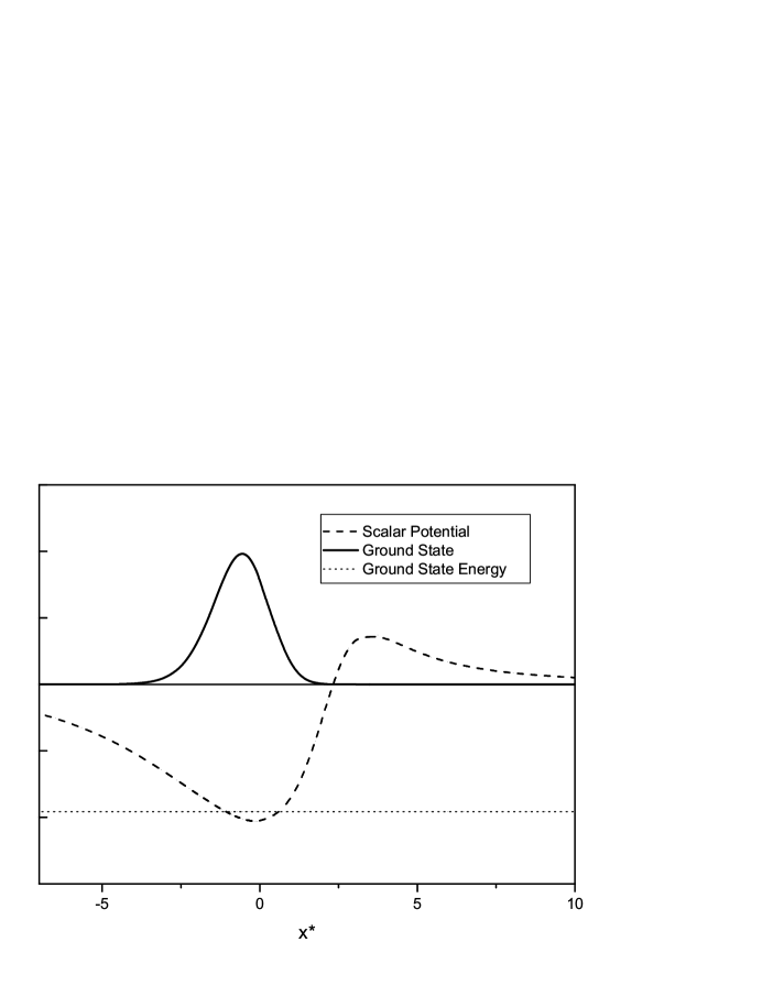
Figure 1: The scalar potential (arbitrary scale) in five dimensions for $\ell=2$ and $\mu/\alpha=1.69$ is shown together with the ground state wave function and energy, found numerically using a shooting algorithm. The origin of $x^{*}$ was chosen as in (17), $x^{*}=0$ for $x=2x_{h}$.

III Tensor mode instability of six dimensional black holes

As in dg1a , we find it convenient to introduce dimensionless variables

$$m:=\mu\alpha^{-3/2},\;\;\;x:=r/(\mu\alpha)^{1/5}=r\alpha^{-1/2}m^{-1/5},\;\;\;dx^{*}/dx:=1/f$$ (32)

The spectrum of the Laplacian on symmetric divergency free tensors on $S^{4}$ is $k_{T}{}^{2}=\ell(\ell+3)-2,\ell\in{\mathbb{Z}}$, only $\ell>1$ tensors being required to construct non trivial tensor perturbations of 6D black holes. These perturbations are entirely described by a single function $\hat{\phi}(t,x)$ governed by an equation that, after separation of variables $\hat{\phi}(t,x)=\phi(x)e^{\omega t}$, assumes the form ${\cal H}_{k_{T}}\psi=-\alpha m^{2/5}\omega^{2}\phi\equiv\alpha m^{2/5}E\phi$ (dg1a , equation (16)), with “Hamiltonian”

$${\cal H}_{k_{T}}=-\frac{\partial^{2}}{\partial x^{*}{}^{2}}+\alpha m^{\frac{2}{5}}V_{k_{T}},$$ (33)

$V_{k_{T}}$ being the RHS of eq. (18) in dg1a . From dg1a we can readily construct the potential, the result is

$$U:=\frac{\alpha V_{k_{T}}}{f}=(k_{T}{}^{2}+2)m^{-\frac{2}{5}}\;U_{o}+m^{-\frac{2}{5}}\;U_{1}+U_{2}-U_{3}$$ (34)

where the $U_{j}$’s depend only on $x$:

$$U_{0} = \frac{2(x^{5}+6)^{2}-75}{2x^{2}(x^{5}+1)(x^{5}+6)}$$ (35)

$$U_{1} = \frac{8\;x^{20}+72\;x^{15}+1218\;x^{10}+1752\;x^{5}-27}{4x^{2}(x^{5}+1)^{2}(x^{5}+6)^{2}}$$ (36)

$$U_{2} = \frac{24\;x^{20}+336\;x^{15}+2414\;x^{10}+2916\;x^{5}+189}{24(x^{5}+1)^{2}(x^{5}+6)^{2}}$$ (37)

$$U_{3} = \frac{24\;x^{20}+216\;x^{15}+1154\;x^{10}+1506x^{5}-81}{24x^{5}(x^{5}+1)^{2}(x^{5}+6)\sqrt{1+6/x^{5}}}$$ (38)

Let $x_{c}=(\sqrt{75/2}-6)^{1/5}\simeq 0.658$ be the only positive root of $U_{o}$, note that $U_{0}<0$ for $0<x<x_{c}$. The $x$ coordinate of the horizon is

$$x_{h}=\frac{z^{2}-4}{2m^{\frac{1}{5}}\;z},\;\;z=\left(2m+2\sqrt{16+m^{2}}\right)^{1/3}.$$ (39)

$x_{h}$ is a monotone increasing function of $m$, and $x_{h}=x_{c}$ at $m=m_{c(6D)}$ given by

$$m_{c(6D)}=\frac{72\sqrt{6}\left(5\sqrt{6}-12\right)^{3/2}}{\left(12-5\sqrt{6}+6^{1/4}\;\sqrt{5}\sqrt{5\sqrt{6}-12}\right)^{5/2}}\simeq 7.965$$ (40)

If $m<m_{c(6D)}$, then $x_{h}<x_{c}$ and we can take a test function supported in $(x_{h},x_{c})$, so that the expectation value of the $U_{0}$ piece of the potential is negative. Note from (34) that this term is proportional to the harmonic $\ell(\ell+3)$, and no other term of ${\cal H}_{k_{T}}$ depends on $\ell$, thus the expectation value of ${\cal H}_{k_{T}}$ for such a test function will be negative for sufficiently high harmonic number. We conclude that 6D BHs are unstable if $m<m_{c}$ above.
Now we prove stability for $m>m_{c(6D)}$: $U_{o},U_{1}$ (and $U_{2}$) are positive if $x>x_{c}$, whereas $U_{2}-U_{3}>0$ if $x>x_{c}^{\prime}\simeq 1.176$. Since $x_{h}=x_{c}^{\prime}$ for $m=m^{\prime}\simeq 48.927$, stability will follow if we prove that $U>0$ for $\ell=2,3...$, $m_{c(6D)}<m<m^{\prime}$ and $x>x_{h}$ given in (39). A lower bound for $U$ in this region of parameter space is given by the minimum of the single variable function $U_{L}:=(10U_{0}+U_{1})50^{-2/5}+U_{2}-U_{3}$ in the interval $x\in(x_{c},\infty)$. After some work $U_{L}$ can be seen to be positive in this interval, thus proving stability. We conclude that 6D BHs are linearly unstable if and only if $\mu/\alpha^{3/2}=m<m_{c(6D)}$.

Fig.2 exhibits the potential and fundamental state (found numerically) corresponding to $\ell=2$, $\mu\alpha^{-3/2}=1.85$.

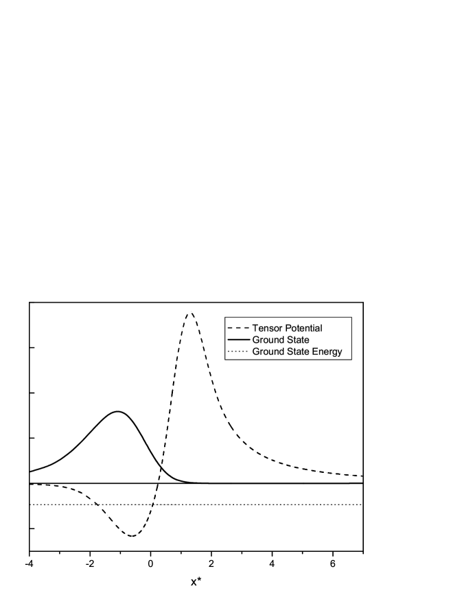
Figure 2: The tensor potential (arbitrary scale) in six dimensions for $\ell=2$ and $\mu\alpha^{-3/2}=1.85$ is shown together with the ground state wave function and energy, found numerically using a shooting algorithm. The origin $x^{*}=0$ corresponds to $x=2x_{h}$.

IV Conclusions

Gauss-Bonnet corrections to Einstein’s equations in higher dimensions have been considered in many different models, and naturally arise in the low energy effective action of certain string theories. However, their effects on black hole formation has long been disregarded. The instability found in dg1a ; dg1b ; dg2 and this paper implies that the simplest EGB black holes (asymptotically Euclidean, static, spherically symmetric), which are the closest analogue of Schwarzschild black holes, cannot actually be formed in five space time dimensions if their mass parameter $\mu$ (see (5)-(6)) is less than $\sim 8.743\alpha$. The Gauss-Bonnet term also prevents the formation of these black holes in six dimensions unless $\mu$ is greater than $\sim 7.965\alpha^{3/2}$. The implications of these figures depend on the context where (4)-(5) is used. As an example, the $n$-dimensional EGB black hole (4)-(5) is an approximate EGB solution if we periodically identify one of the asymptotically Euclidean coordinates with a period much larger than the horizon radius, and our perturbative analysis should be valid in this setting. The large extra dimensions scenario (suitable only for $D\geq 6$, alexeyev ) is of interest because it allows $\alpha$ to be in the TeV scale alexeyev ; otros , and so mini black holes could be produced in high energy collisions and be eventually detected at LHC. In view of our results, the probability of these events may be severely limited due to low mass black hole instabilities. As far as we know, this fact has not been taken into account in previous calculations on black hole production rates in high energy collisions. In theories where the EGB equations simply arise as a low energy effective theory of some quantum gravity model, $\alpha$ is of the order of the Planck scale and the bounds we obtained for small black hole masses are much more stringent.

References

• (1) D. Lovelock, Jour. Math. Phys. 12 (1971) 498.
• (2) M. J. Duff, B. E. W. Nilsson and C. N. Pope, Phys. Lett.  B 173, 69 (1986); D. J. Gross and E. Witten, Nucl. Phys. B277, 1 (1986); B. Zumino, Phys. Rep. 137, 109 (1985); B. Zwiebach, Phys. Lett. 156B, 315 (1985); D. Friedan, Phys. Rev. Lett. 45 (1980) 1057; I. Jack, D.Jones and N. Mohammedi, Nucl. Phys. B322, 431 (1989); C. Callan, D. Friedan, E. Martinec and M. Perry, Nucl. Phys. B262, 593 (1985).
• (3) D. G. Boulware and S. Deser, Phys. Rev. Lett.  55, 2656 (1985).
• (4) J. T. Wheeler, Nuc. Phys. B268 (1986) 737
• (5) J. T. Wheeler, Nuc. Phys. B273 (1986) 732.
• (6) R. C. Myers and J. Z. Simon, Phys. Rev.  D 38 (1988) 2434.
• (7) R. C. Myers and M. J. Perry, Annals Phys.  172, 304 (1986).
• (8) G. Dotti and R. J. Gleiser, Class. Quant. Grav.  22 (2005) L1 [arXiv:gr-qc/0409005].
• (9) F.R. Tangherlini, Nuovo Cimento 27, 365 (1963).
• (10) G. Dotti and R. J. Gleiser, Phys. Rev. D 72 (2005) 044018 [arXiv:gr-qc/0503117].
• (11) R. J. Gleiser and G. Dotti, Phys. Rev. D 72 (2005) 124002 [arXiv:gr-qc/0510069].
• (12) G. Gibbons and S. A. Hartnoll, Phys. Rev.  D 66 (2002) 064024 [arXiv:hep-th/0206202].
• (13) H. Kodama, A. Ishibashi and O. Seto, Phys. Rev. D62 (2000) 064022.
H. Kodama and A. Ishibashi Prog.Theor.Phys. 111 (2004) 29, hep-th/0308128; H. Kodama and A. Ishibashi, gr-qc/0312012.
• (14) T. Regge and J. A. Wheeler, Phys. Rev. 108 (1957) 1063.
• (15) A. Higuchi, J. Math. Phys. 28 (1987) 1553; J. Math. Phys. 43 (2002) 6385 (erratum); M. A. Rubin and C. R. Ordoñez, J. Math. Phys.  26 (1985) 65.
• (16) R. J. Gleiser and G. Dotti, Class. Quant. Grav.  23, 5063 (2006) [arXiv:gr-qc/0604021].
• (17) S. Alexeyev, A. Barrau and J. Grain, Proceedings of Quarks-2004, 13th International Seminar on High Energy Physics, Pushkinskie Gory, Russia, May 24-30, 2004; S.Alexeyev, N.Popov, A.Barrau and J.Grain, Journal of Physics: Conference Series 33 (2006) 343 348.
• (18) N. Arkani-Hamed, S. Dimopoulos and G.R. Dvali, Phys. Lett. B 429 (1998) 257 I. Antoniadis et al., Phys. Lett. B 436 (1998) 257 N. Arkani-Hamed, S. Dimopoulos and G.R. Dvali, Phys. Rev. D 59 (1999) 086004.