We explain how to construct a large class of new quiver gauge theories from branes at singularities by orientifolding and Higgsing old examples. The new models include the MSSM, decoupled from gravity, as well as some classic models of dynamical SUSY breaking. We also discuss topological criteria for unification.

1. Introduction

1.1. Overview: merits of local constructions

String theory grew out of a desire to provide a framework for particle physics beyond the Standard Model and all the way up to the Planck scale. In order to make progress, one needs to find an embedding of the SM, or some realistic extension such as the MSSM, in ten-dimensional string theory. A beautiful aspect of such a picture is that the details of the matter content and the interactions are governed by the geometry of field configurations in the six additional dimensions.

The main approaches that have been considered are

• Heterotic strings;

• Global D-brane constructions;

• Local D-brane constructions.

Here we have distinguished two kinds of D-brane constructions. By a local construction we mean a construction which satisfies a correspondence principle: we require that there is a decoupling limit in which the 4D Planck scale goes to infinity, but the SM couplings at some fixed energy scale remain finite. This requirement is motivated by the existence of a large hierarchy between the TeV scale and the Planck scale. The natural set-up which satisfies this principle is fractional branes at a singularity.

Figure 1: Caricature of a global D-brane model. If the size of the $T^{2}$ goes to infinity, as typically happens in the $M_{\rm pl,4}\to\infty$ limit, the volumes of the branes and the distance between their intersections goes to infinity as well, shutting of the Standard Model couplings.

Our use of the words ‘local construction’ differs from some of the literature. In global constructions the SM fields are often also localized in ten dimensions, but in the $M_{\rm Pl,4}\to\infty$ limit most of the Standard Model interactions are turned off. This is because either the cycle on which a brane is wrapped becomes large, turning off the gauge coupling, or because fermion and scalar wave functions are supported on regions which get infinitely separated in this limit, turning off Yukawa couplings. Similarly in the heterotic string, the perturbative gauge interactions are shut off if we take the volume of the Calabi-Yau to infinity. We will require that all these interactions remain finite in the decoupling limit.

We cannot guarantee that the correspondence principle is satisfied in nature. However we believe that insisting on it is an important model building ingredient, if only to disentangle field theoretic model building issues from quantum gravity. In addition, insisting on such a scenario has a number of practical advantages:

• Holography: Higher energy scales in the gauge theory correspond to probing distances farther away from the brane. This property allows one to take a bottom-up perspective to model building [1]. In order to reproduce the SM we only need to know a local neighbourhood of the brane of radius $r$, where $U=r/\alpha^{\prime}\sim 1\,{\rm TeV}$.

• Adjustability: The couplings of the gauge theory translate to boundary values of closed string fields on the boundary of this local neighbourhood, and we may adjust them at will. Their values are set by some high energy physics which we have not yet included.

• Uniqueness: It is expected that the closed string theory can be recovered from the open string theory. So up to some natural ambiguities like T-dualities, the local neighbourhood should be completely determined by the ensemble of gauge theories obtained by varying the ranks of the gauge groups. Thus finding the local geometry for a gauge theory is a relatively well-posed problem which should have a unique solution. The apparent non-uniqueness seen in other approaches is reflected here in the fact that there might be many different extensions of the same local geometry.

In [2] Herman Verlinde and the author gave a construction of a local model resembling the MSSM. This construction had some drawbacks which could be traced back to the fact that we were working with oriented quivers. In this paper we address the problem of giving a local construction of the MSSM itself.

We have frequently seen the sentiment expressed that gauge theories obtained from branes at singularities are somehow rather special. The main message of this paper is not so much that we can construct some specific models. Rather it is that with the present set of ideas we can get pretty much any quiver gauge theory from branes at singularities. To illustrate this point, we also engineer some classic models of dynamical SUSY breaking.

While we touch on some more abstract topics like exceptional collections, the strategy is really very simple. We look for an embedding of the MSSM into a quiver gauge theory for which the geometric description is known, and then turn on various VEVs and mass terms. In order to keep maximum control we require the deformations to preserve supersymmetry. Below the scale of the masses, we can effectively integrate out and forget the extra massive modes. On the geometric side, this corresponds to turning on certain moduli of the fractional brane or changing the complex structure of the singularity, and cutting off the geometry below the scale of the superfluous massive modes. Hence we can speak of the geometry of the MSSM.

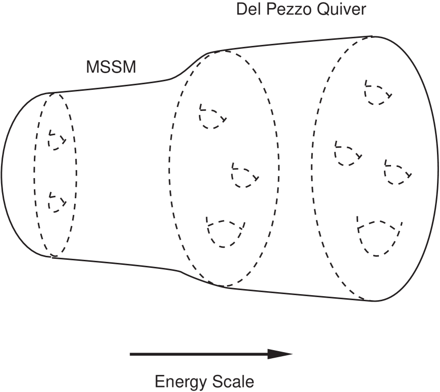
Figure 2: The radial direction away from the fractional brane is interpreted as an energy scale. After Higgsing the Del Pezzo quiver theory, a sufficiently small neighbourhood of the singularity describes the MSSM.

The Del Pezzo quiver and other intermediate quivers are purely auxiliary theories which are possible UV extensions of the MSSM. Our construction appears to be highly non-unique. This is a reflection of the bottom-up perspective, in which the theory can be extended in many ways beyond the TeV scale.

While we don’t believe it is an issue, we should mention a possible caveat in our construction. As we will review we can vary superpotential terms in the original Del Pezzo quiver independently, and it is expected but not completely obvious that the same is true in the Higgsed superpotential. One would like to prove that one can vary mass terms independently so that we can keep some non-chiral Higgs fields light and the remainder arbitrarily heavy. We checked on the computer in a number of simple examples that it works as expected. However in our realistic examples some of the mass terms in the Higgsed quiver should be induced from superpotential terms in the original Del Pezzo quiver which are of 12th order in the fields. Unfortunately due to memory constraints we have only been able to handle 4th and 8th order terms on the computer, and so we have not explicitly shown in these examples that all excess non-chiral matter can be given a mass.

1.2. The MSSM as a quiver

Let us now describe what we mean by obtaining the MSSM. With D-branes, the best one can do is obtaining the MSSM together with an additional massive gauge boson. In addition, the right-handed neutrino sector is not set in stone. We first describe the quiver we would like to produce. In later sections, we describe how to engineer it.

Any weakly coupled D-brane construction of the MSSM will have at least one extra massive gauge boson, namely gauged baryon number, because the $SU(3)_{\rm colour}$ always gets enhanced to $U(3)$. In addition, we have to choose how to realize the right-handed neutrino sector. The most likely sources for right-handed neutrinos are:

• open strings charged with respect to a gauge symmetry that is not part of the SM;

• uncharged open strings;

• superpartners of closed string moduli.

Since all such modes are singlets under the observed low energy gauge groups, they will probably mix and there may not be an invariant distinction between them.

One of the closest quivers we could try to construct is shown in figure 3A.

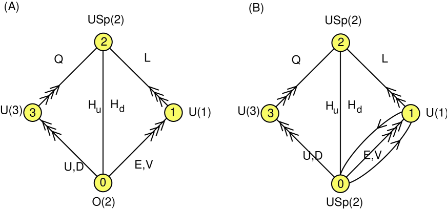
Figure 3: (A): An MSSM quiver, with an additional massless $U(1)_{B-L}$. (B): Model I, a left-right unified model which can be Higgsed to the MSSM.

This is essentially the ‘four-stack’ quiver first discussed in [5]. It consists of the MSSM plus $U(1)_{B}$ and $U(1)_{L}$ vector bosons, and a right-handed neutrino sector from charged open strings. Many groups have searched for this model and closely related ones in specific compactifications, see for instance [6, 7] and the review [8].

The combination $U(1)_{B+L}$ is anomalous, and as usual gets a mass by coupling to a closed string axion (the Stückelberg mechanism). Note this is not the PQ axion, which may or may not exist, depending on the UV extension of the local geometry. The combination $U(1)_{B-L}$ is not anomalous, but could still get a mass by coupling to a closed string axion, also depending on the UV completion. However if we take the gauge group on the bottom node to be literally $O(2)$, i.e. obtained from an orientifold projection of $U(2)$, then this $O(2)$ can not have a Stückelberg coupling to an axion. Since we would like to keep a massless $U(1)_{Y}$, and since $U(1)_{Y}$ is a linear combination of the $SO(2)$ and $U(1)_{B-L}$, this means that $U(1)_{B-L}$ cannot get a mass through the Stückelberg mechanism.

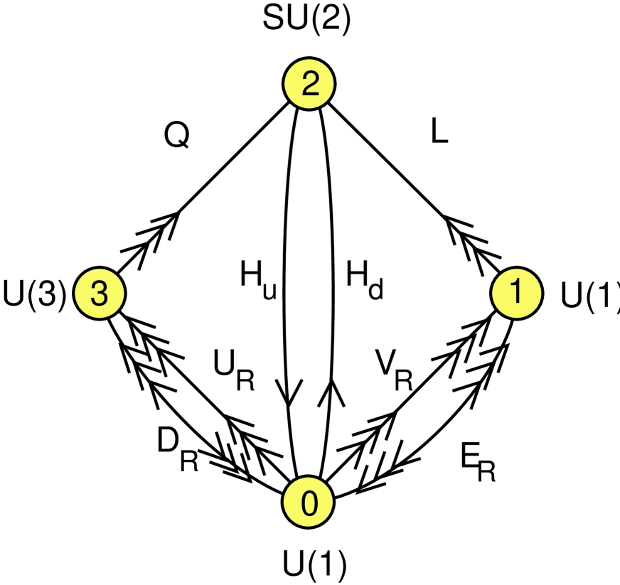
Figure 4: Model II: a quiver consisting of the MSSM, $U(1)_{B-L}$ plus a massive $U(1)_{B+L}$. The $U(1)_{B-L}$ can be coupled to a Stückelberg field.

Thus we have two options. Either we instead construct the orientifold model in figure 4, where the $U(1)$ on the bottom node comes from identifying two different nodes on the covering quiver. Then we have recourse to the Stückelberg mechanism to get rid of $U(1)_{B-L}$. We will call this quiver model II. A construction of this model is given in section 4.3.

Alternatively we can make the extra $U(1)$ massive by conventional Higgsing. This requires adding some non-chiral matter and condensing it, or turning on a VEV for a right handed s-neutrino. In this case, we would finally end up with the quiver in figure 5. This quiver consists of the MSSM, together with a massive $U(1)_{B}$ gauge boson, and a right-handed neutrino sector from uncharged open strings (adjoints).

If in fact we use the second option, adding non-chiral matter and Higgsing, then for our purposes here we might as well replace the $O(2)$ with a $USp(2)$, since both break to the same model up to some massive particles. In the local set-up, the masses of the extra particles may be taken arbitrarily large. Moreover up to the massive $U(1)_{B}$ this is actually a well known unified model, the minimal left-right symmetric model (an intermediate step to $SO(10)$ unification), so it has some independent interest. Thus we might as well construct the quiver in figure 3B, which we will call model I. This is the simpler of the constructions in this paper, and will be explained in section 4.1.

We should point out that $R$-parity is not quite automatic in either of our models, although both models appear to have a global $U(1)_{B-L}$. In our first model we must preserve $R$-parity in our final Higgsing to the MSSM. In both models we might need to worry about $D$-instanton effects which break this symmetry after coupling to 4D gravity, though such effects are presumably small. This is not really surprising: the MSSM does not explain $R$-parity, it merely assumes it. To explain it, we must know more about the UV extension of our models.

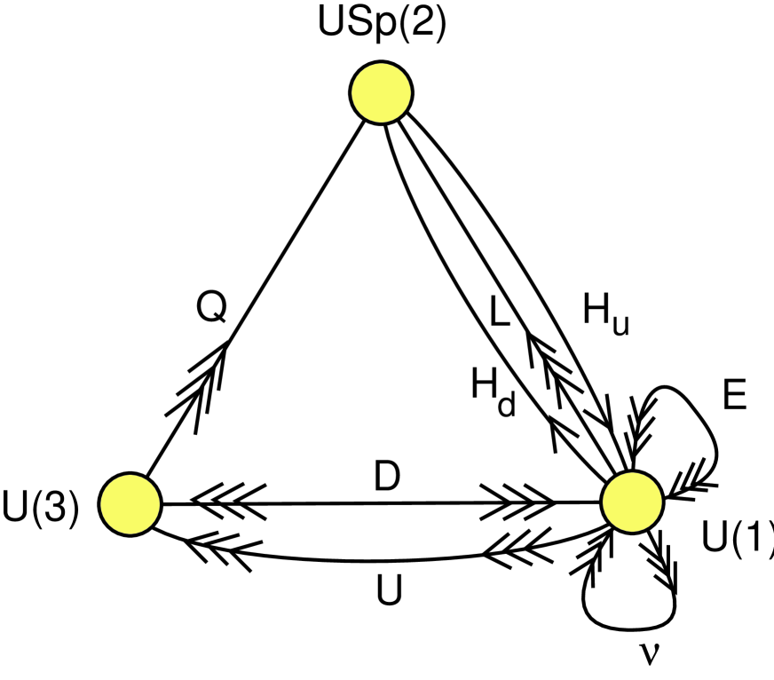
Figure 5: The Standard model plus $U(1)_{B}$. Note we still need R-parity to forbid undesirable couplings.

Now to get a hint for finding these quivers, we first draw the oriented covering quivers. The covering quiver for the quivers in figure 3 is drawn in figure 6A, and the covering quiver for figure 4 is given in figure 6B.

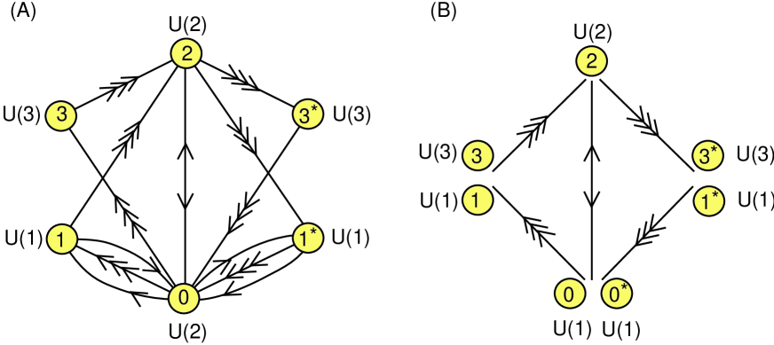
Figure 6: (A): Covering quiver of model I. (B): Covering quiver of model II. In (B) we have grouped nodes together if they have the same intersection numbers with all other nodes, to make the diagram less cluttered.

These quivers have to our knowledge not yet been encountered in the literature on D-branes at singularities. Although the number of generations doesn’t match, these quivers still bear a close resemblance to the characteristic structure of Del Pezzo quivers, and especially to Del Pezzo 5. Recall that a Del Pezzo singularity is a Calabi-Yau singularity with a single Del Pezzo surface collapsing to zero size. The Del Pezzo surfaces are ${\bf P}^{1}\times{\bf P}^{1}$ or ${\bf P}^{2}$ blown up at up to eight points. We will give a discussion of orientifolds of Del Pezzo 5 (i.e. five blow-ups of ${\bf P}^{2}$) in section 3.

1.3. Why Del Pezzo surfaces?

The fact that the Del Pezzo quivers are seen to be relevant is not surprising. It is practically guaranteed when we ask for chiral gauge theories which are not too complicated. Let us explain this point.

Any $CY_{3}$ singularity has a collection of 2- and 4-cycles collapsing to zero size. Now chiral matter comes from intersection of 2-cycles with 4-cycles. This is easy to see: for instance if we have only branes wrapping 2-cycles, we can always deform the branes (at some cost in energy) so that they don’t intersect. Then all open string modes are massive, and thus the net number of chiral fermions must be zero. So requiring chiral fermions implies that we have to have some collapsing 4-cycles in the geometry. The Del Pezzo singularities, which have precisely a single collapsing 4-cycle, are then the simplest examples.

Moreover, a minimal D-brane realization of the SM has one local $U(1)$ which is anomalous, namely $U(1)_{B}$, and this lifts to two anomalous $U(1)$’s on the oriented covering quiver. Now the the number of anomalous $U(1)$’s is interpreted geometrically as the rank of the intersection matrix of vanishing cycles. Hence the Del Pezzo quivers and their orientifolds are natural candidates because they are chiral quivers with the minimum number of anomalous $U(1)$’s, namely two.

Although the models we are looking for are not among the known Del Pezzo quivers, these arguments convinced us that we should derive them from the quivers that were already known, rather than look for new singularities.

2. Lightning review of branes at singularities

Consider a Calabi-Yau singularity in IIb string theory, characterized by a collection of vanishing 2- and 4-cycles. Since the curvature is very large, it is in general not clear how to define the notion of a D-brane at a singularity. An notable exception is the case of orbifold singularities, where we can use free field theory. From this special case the following picture has emerged: given a singularity we expect the existence of a finite set of irreducible “fractional” branes. For the case of orbifolds these irreducible branes are in one-to-one correspondence with the irreducible representation of the orbifold group. To these irreducible branes we can associate the basic quiver diagram. For each irreducible fractional brane we draw a node, and for each massless open string which goes from brane $i$ to brane $j$ we draw an arrow or an edge between the corresponding nodes. All the remaining branes can be expressed as bound states of these irreducible branes, or equivalently as a Higgsing of the basic quiver.

Now how do we find the basic quiver for a general singularity? Let us assume our branes are half BPS and space-time filling, so that we get a 4D $N=1$ quiver gauge theory. Then we can use the following strategy: we make sure that the F-term equations are satisfied, but we temporarily ignore the D-term equations. Then we can blow up the vanishing 2- and 4-cycles and extrapolate to the large volume limit (figure 7). This limit is unphysical from the point of view of the quiver gauge theory, because the D-terms are not satisfied, but in this limit we understand how to compute the F-term equations. Moreover due to the shift symmetry of the $B$-field we can argue that the perturbative superpotential does not depend on complexified Kähler moduli and must be the same as in the small radius limit. When the cycles are large and the curvature is small, we can represent the D-branes by sheaves localized on the vanishing cycles. The irreducible fractional branes get mapped to an exceptional collection $\{F_{1},\ldots,F_{n}\}$, that is a collection of rigid bundles whose relative Euler characters $\chi(F_{i},F_{j})$ form an upper-triangular matrix.

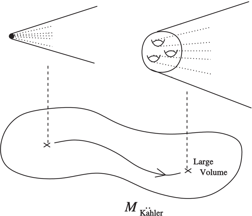
Figure 7: Ignoring the D-terms and extrapolating to the large volume limit.

The exceptional collections have been worked out for many interesting singularities. For the purpose of this paper all that we are going to need is the charge vector or Chern character ${\rm ch}(F_{i})$ of the branes in the exceptional collection. The Chern character of a sheaf tells us the rank, the fluxes, and the instanton number, in other words it tells us the effective (D7,D5,D3) wrapping numbers of the fractional brane.

Thus to an exceptional collection we can associate a quiver diagram. Each sheaf in the collection corresponds to an irreducible fractional brane, and thus to a node. The net number of chiral fields between two nodes is simply the net intersection number of the cycles that the fractional brane wraps. We can put this in the form of a matrix, the adjacency matrix of the quiver. In the case of collapsed 4-cycles this is just the anti-symmetrization $\chi_{-}(F_{i},F_{j})$ of the upper-triangular matrix of the collection. The non-chiral matter can be obtained by a slightly more refined cohomology computation.

As mentioned we can also reconstruct other F-term data such as the superpotential. The physicists method is to compute some correlation functions of the chiral fields. The mathematicians method is to first compute the dual exceptional collection, whose relative Euler characters are given by the inverse of the above mentioned upper-triangular matrix. The superpotential now follows from the relations in the path algebra of the dual collection.

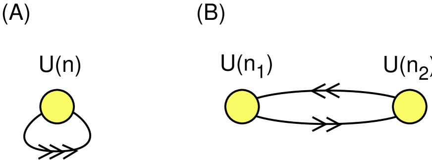
Figure 8: (A): Quiver for $N=4$ Yang-Mills theory. (B): Quiver for the conifold.

The superpotential encodes all of the complex geometry of the Calabi-Yau singularity. This complex geometry is generically non-commutative. Let us consider for example pure $N=4$ Yang-Mills theory. Its quiver is a single node with 3 arrows back to itself. The superpotential is

$$W={1\over 6}\,\epsilon_{ijk}\,{\rm Tr}(Z^{i}Z^{j}Z^{k})\qquad i,j,k=1,2,3.$$ (2.1)

The $Z^{i}$’s are matrices after we assign gauge group ranks to the nodes, but let us temporarily treat them as formal non-commuting variables. The F-term equations then tell us that

$$\frac{1}{2}\epsilon_{ijk}\,Z^{i}Z^{j}=0$$ (2.2)

in other words the Calabi-Yau is a commutative ${\bf C}^{3}$. However we may perturb the superpotential, for instance by adding mass terms

$$W={1\over 6}\,\epsilon_{ijk}\,{\rm Tr}(Z^{i}Z^{j}Z^{k})+\frac{1}{2}m_{kl}\,{\rm Tr}(Z^{k}Z^{l}).$$ (2.3)

The new F-term equations tell us that

$$\frac{1}{2}\epsilon_{ijk}Z^{i}Z^{j}=m_{kl}Z^{l}$$ (2.4)

In other words, we may deform ${\bf C}^{3}$ to a generic 3-dimensional Lie algebra. This illustrates another important point that we also emphasized in the introduction. The quiver gauge theory itself is in fact the best definition of the local geometry.

As another example, let us consider the quiver for the conifold. It has a superpotential

$$W={\rm Tr}(A^{i}B^{k}A^{j}B^{l})\,\epsilon_{ij}\epsilon_{kl},\qquad i,j,k,l=1,2.$$ (2.5)

If we define

$$z_{1}=A^{1}B^{1},\quad z_{2}=A^{1}B^{2},\quad z_{3}=A^{2}B^{1},\quad z_{4}=A^{2}B^{2}$$ (2.6)

then the F-term equations tell us that

$$z_{i}z_{j}-z_{j}z_{i}=0,\quad z_{1}z_{4}-z_{2}z_{3}=0.$$ (2.7)

Superpotential deformations correspond to deformations of these equations. For instance we could turn on mass terms

$$W\to W+m_{ij}\,{\rm Tr}(A^{i}B^{j}).$$ (2.8)

This leads to the relations

$$\begin{array}[]{rclrcl}z_{1}z_{2}-z_{2}z_{1}&=&m_{21}z_{1}+m_{22}z_{2}&z_{2}z_{3}-z_{3}z_{2}&=&m_{22}z_{4}-m_{11}z_{1}\\ z_{3}z_{1}-z_{1}z_{3}&=&m_{12}z_{1}+m_{22}z_{3}&z_{2}z_{4}-z_{4}z_{2}&=&m_{11}z_{2}+m_{21}z_{4}\\ z_{1}z_{4}-z_{4}z_{1}&=&m_{12}z_{2}-m_{21}z_{3}&z_{4}z_{3}-z_{3}z_{4}&=&m_{11}z_{3}+m_{12}z_{4}\\ &&&z_{1}z_{4}-z_{2}z_{3}&=&-m_{11}z_{1}-m_{12}z_{2}\end{array}$$ (2.9)

This ‘massive conifold’ is the analogue of the $N=1^{*}$ deformation of $N=4$ Yang-Mills theory. Actually this is only part of the story, because the superpotential is modified quantum mechanically. In the IR both gauge groups will confine and lead to glueball condensates. Presumably this leads to a combination of a conifold transition and a Myers effect. This theory exhibits many further interesting effects like meta-stable vacua. Surprisingly it has received no attention in the literature and we are further investigating it [11].

More generally, we will be interested in adding irrelevant terms to the superpotential. These clearly correspond to subleading complex structure deformations of the singularity.

The physical intuition is that closed string modes are in one-to-one correspondence with general gauge invariant deformations of the quiver. For superpotential deformations this has been put on a firm footing by Kontsevich [12], who shows that infinitesimal deformations of the “derived category” (i.e. single trace superpotential deformations) correspond to observables in the closed string B-model. In the context of mirror symmetry, the significance of this statement is that together with a corresponding statement for the A-model, it provides evidence for the correspondence principle, i.e. the idea that classical mirror symmetry can be recovered from homological mirror symmetry.

As we explained, our main interest will be in the Del Pezzo quivers. The first five Del Pezzo quivers were found using orbifold and toric techniques [13, 14, 15, 16, 17]. Some of these were rederived using exceptional collections in [18, 19], and finally the remaining five non-toric Del Pezzo quivers, including Del Pezzo 5 which will play a central role in this paper, were found using exceptional collections [20]. We refer to [20, 21] for more detailed reviews and explicit computations. For other interesting works we refer to [22, 23, 24, 25, 26].

3. Orientifolding quivers

Discussions of orientifolds and derived categories have recently been given in the LG regime [27] and in the large volume regime [28]. Here we describe orientifolds in another regime, which is captured by quiver gauge theories. Traditionally orientifolds of branes at singularities have been derived by first specifying an orientifold action on the closed string modes, and then finding the induced action on open string modes. Here we start by specifying an orientifold action on the open string modes. This simplifies the task of finding a brane realization of a desired gauge theory, and at any rate the closed string geometry can be reconstructed from the gauge theory.

3.1. General discussion of orientifolding

Perturbative string theory on IIb backgrounds has a number of $Z_{2}$ symmetries. They include $(-1)^{F_{L}}$ and worldsheet parity $P$. In addition, on a given background the theory may have an additional $Z_{2}$ symmetry $\sigma$.

Given such a symmetry, we can construct a new perturbative string background by gauging it. An orientifold projection is an orbifold which involves $P$. In addition, we would like to preserve $N=1$ SUSY in four dimensions. Recall that in IIB string theory on a Calabi-Yau the supercharges with positive 4D chirality are derived from the currents

$$j^{1}_{\alpha}=e^{-\varphi_{L}/2}\,S_{L\alpha}\,e^{{1\over 2}\int J_{L}},\qquad j^{2}_{\alpha}=e^{-\varphi_{R}/2}\,S_{R\alpha}\,e^{{1\over 2}\int J_{R}},$$ (3.1)

where in the large volume limit

$$e^{\int J_{L}}=\Omega^{(3,0)}_{ijk}\psi_{L}^{i}\psi_{L}^{j}\psi_{L}^{k},\qquad e^{\int J_{R}}=\Omega^{(3,0)}_{ijk}\psi_{R}^{i}\psi_{R}^{j}\psi_{R}^{k}.$$ (3.2)

We have used the conventional notations for the bosonized superghost, 4D spin fields and wordsheet fermions. In type IIa, the second current would have been proportional to the square root of $\bar{\Omega}^{(0,3)}_{\bar{i}\bar{j}\bar{k}}\psi^{\bar{i}}_{R}\psi^{\bar{j}}_{R}\psi^{\bar{k}}_{R}$, because the second spinor must have negative 10D chirality. In order to preserve SUSY there must be a linear combination that is preserved. If we do not include $(-1)^{F_{L}}$, then

$$Q^{1}_{\alpha}+Q^{2}_{\alpha}$$ (3.3)

is preserved under orientifolding, provided $\sigma$ is a symmetry of the internal CFT that maps $\Omega^{(3,0)}\to\Omega^{(3,0)}$. If we instead include $(-1)^{F_{L}}$ in the orientifolding, then

$$Q^{1}_{\alpha}-iQ^{2}_{\alpha}$$ (3.4)

is preserved under orientifolding, provided $\sigma$ maps $\Omega^{(3,0)}\to-\Omega^{(3,0)}$.

Parity exchanges the Chan-Paton factors at the ends of an open string, and acts as $-1$ on massless open string modes, so it maps gauge fields and chiral fields to minus their transpose. We are interested in local orientifold models, so we will be looking for symmetries of the quiver of irreducible branes which map a gauge field at node $i$ to minus the transpose of the gauge field at some node $j$, and map any chiral field $X$ to the transpose $Y^{T}$ of some other chiral field, possibly up to an additional gauge transformation which we call $\gamma$. We denote this as $i\leftrightarrow j^{*}$. In our decoupling limit, finding such a symmetry is sufficient, because the irreducible branes generate all other branes and closed strings ought to be recovered from open strings. In particular we can read of the local geometry from the gauge invariant operators and their relations.

We will assume canonical kinetic terms for the chiral fields, so we can actually map $X\to e^{i\varphi}Y^{T}$ for some phase $\varphi$. If there are multiple arrows between two nodes, we can upgrade the map to a unitary matrix. In order to preserve SUSY, the orientifold action has to leave the superspace coordinate $\theta$ invariant, and hence it will also have to leave the superpotential invariant. This may lead to correlations between the $SO$ and $Sp$ projections on different nodes, and symmetric or anti-symmetric projections on chiral fields that are mapped to themselves.

One should keep in mind that a non-anomalous quiver theory may become anomalous after projection if the ranks of the gauge groups are not adjusted. The orientifold may project out more of the positive than of the negative contributions to an anomaly. This is generically the case if the projected theory contains symmetric and anti-symmetric tensor matter. From the geometric point of view, this is because an orientifold plane may give additional tadpole contributions, which need to be cancelled by adding additional branes, i.e. adjusting the ranks of the gauge groups.

We can also understand how the orientifold acts on closed string modes. The modes that are kept are simply the closed string modes on the cover that can be used to deform the orientifolded theory. To preserve SUSY, the orientifold action maps $\tau_{i}\to\tau_{j^{*}}$ and $L_{i}\to-L_{j^{*}}$, where $\tau$ denotes the complexified gauge coupling and $L$ denotes the linear multiplet containing the FI parameter and the Stückelberg 2-form field.

3.2. Examples

Orientifold of ${\bf P}^{2}$

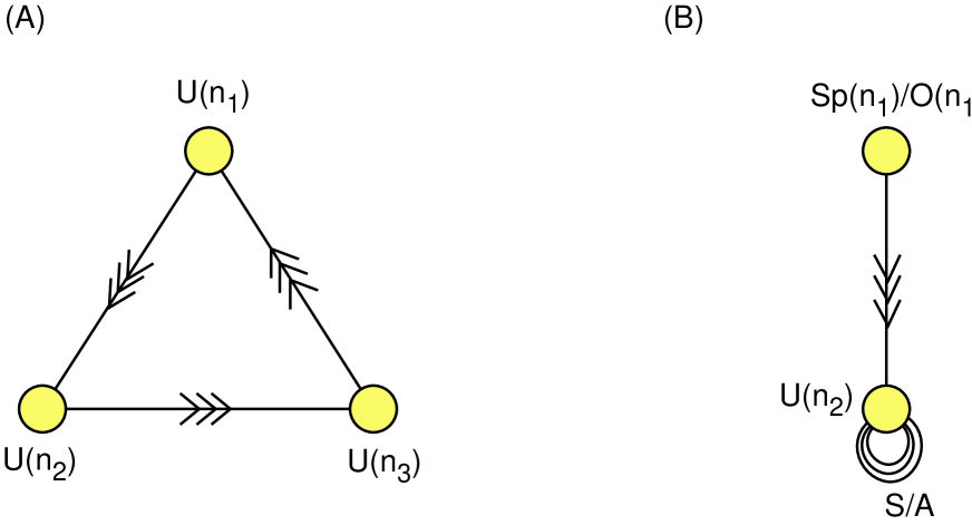
Figure 9: (A) Quiver for ${\bf P}^{2}$. (B) Orientifold.

The simplest case to understand is the Calabi-Yau cone over ${\bf P}^{2}$, which is identical to the orbifold singularity ${\bf C}^{3}/Z_{3}$. This orientifold is already known in the literature [29], but we will use a slightly more geometric perspective. We denote the hyperplane class by $H$. The quiver is given in figure 9A and may be obtained from a set of fractional branes with the following (D7,D5,D3) wrapping numbers:

$$1.\ (1,0,0)\quad 2.\ -(2,H,-\frac{1}{2})\quad 3.\ (1,H,\frac{1}{2}).$$ (3.5)

We consider the following symmetry:

$$1\leftrightarrow 1^{*},\quad 2\leftrightarrow 3^{*}.$$ (3.6)

We may take an $Sp$- or $SO$-projection. Assuming the usual orbifold superpotential, the matter between nodes 2 and 3 projects to a conjugate symmetric tensor (for $Sp$) or a conjugate anti-symmetric tensor (for $SO$). The orientifolded quiver is given in figure 9B.

We expect an orientifold plane which coincides with the fractional brane on node 1, i.e. it is an O7-plane wrapped on the vanishing Del Pezzo. Anomaly cancellation implies that $n_{1}=n_{2}+4$ for symmetric tensor matter, and $n_{1}=n_{2}-4$ for anti-symmetric tensor matter. In order to cancel the flux through the hyperplane class, we take the charge vector of the O7-plane to be $(\mp 4,0,0)$. We don’t guarantee however that there are no further O3-plane charges.

In the geometric regime the net number of symmetric and anti-symmetric matter is given by [30]

$$\#\ {\rm sym} \!\!=\!\! \frac{1}{2}I_{nn^{*}}+{1\over 8}I_{nO}$$

$$\#\ {\rm asym} \!\!=\!\! \frac{1}{2}I_{nn^{*}}-{1\over 8}I_{nO}$$ (3.7)

where $I_{ij}$ is the intersection form of the Calabi-Yau. We expect this formula also for small volume, and indeed it agrees with the spectrum above. However it is not always clear what charges we should assign to an orientifold plane. The guiding principle is that we get a sensible gauge theory in which all anomalies are cancelled, and from that we may try to reconstruct the orientifold plane.

The proposed O7-plane is not the fixed locus of any $Z_{2}$ after blowing up, so we believe that the large volume limit is projected out. There are other ways to see this. The definition of the orientifold which produces this quiver involves a symmetry which interchanges oppositely twisted sectors, which is not available after blowing up. There is no symmetry that maps a rank 2 bundle to a rank 1 bundle in the geometric regime. And the orientifold imposes relations on the gauge couplings of nodes $2$ and $3$, which in turn freezes the Kähler modulus.

The case of the $SO$ projection with $n_{2}=5$ gives us a simple 3-generation $SU(5)$ GUT with a $\bar{5}$ and a $10$ from the anti-symmetric [29]. There are no Higgses, though they could presumably be generated by first increasing the ranks and then Higgsing. Of course there would be well-known problems with getting the ${5}\times 10\times 10$ Yukawa’s. This model also exhibits dynamical SUSY breaking [29], but with a runaway behaviour.

Orientifold of ${\bf P}^{1}\times{\bf P}^{1}$

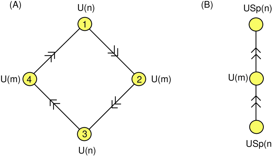
Figure 10: (A) Quiver for ${\bf P}^{1}\times{\bf P}^{1}$. (B) Orientifold.

The next interesting case is ${\bf P}^{1}\times{\bf P}^{1}$. This example is very similar to the ${\bf C}^{3}/Z_{4}$ orbifold singularity, to which it is related by turning on masses for the non-chiral fields and flowing to the IR. We denote the first ${\bf P}^{1}$ by $H_{1}$ and the second by $H_{2}$. Their intersection numbers, when restricted to ${\bf P}^{1}\times{\bf P}^{1}$, are

$$H_{1}\cdot H_{1}=H_{2}\cdot H_{2}=0,\quad H_{1}\cdot H_{2}=1.$$ (3.8)

The quiver is shown in figure 10 and can be obtained from an exceptional collection with the following $(D7,D5,D3)$ wrapping numbers:

$$1.\ (1,0,0)\qquad 2.\ -(1,H_{1},0)\qquad 3.\ -(1,H_{2}\!-\!H_{1},1)\qquad 4.\ (1,H_{2},0)$$ (3.9)

We are interested in the following orientifold action:

$$1\leftrightarrow 1^{*}\qquad 2\leftrightarrow 4^{*}\qquad 3\leftrightarrow 3^{*}$$ (3.10)

and

$$X_{12}^{T}\gamma_{1}=X_{41},\qquad Y_{12}^{T}\gamma_{1}=Y_{41},\qquad\gamma_{3}^{-1}X_{23}^{T}=X_{34},\qquad\gamma_{3}^{-1}Y_{23}^{T}=Y_{34}.$$ (3.11)

As usual we have

$$\gamma_{1}^{T}=s(1)\cdot\gamma_{1},\qquad\gamma_{3}^{T}=s(3)\cdot\gamma_{3}$$ (3.12)

with $s=\pm 1$, in order for the action on the gauge fields to be an involution. The superpotential of the commutative ${\bf P}^{1}\times{\bf P}^{1}$ quiver is

$$W=X_{12}X_{23}X_{34}X_{41}-X_{12}Y_{23}X_{34}Y_{41}+Y_{12}Y_{23}Y_{34}Y_{41}-Y_{12}X_{23}Y_{34}X_{41}.$$ (3.13)

In order for this particular superpotential to be invariant, we also need

$$s(1)\cdot s(3)=+1$$ (3.14)

so we can have an $SO/SO$ or an $Sp/Sp$ projection. More generally we could work the other way around. We first decide on the projections that we would like to have, and then we write down the most general superpotential compatible with those projections.

The orientifold locus appears to consist of the union of two O7-planes, with wrapping numbers $4(1,0,0)$ and $-4(1,H_{2}\!-\!H_{1},1)$. This is not the fixed locus of any $Z_{2}$ symmetry after blowing up, so the large volume limit is projected out.

Orientifold of Del Pezzo 5

Now we come to the main case of interest, the Del Pezzo 5 singularity. The Del Pezzo 5 surface is a ${\bf P}^{2}$ blown up at five generic points. As a basis for the 2-cycles we use the hyperplane class $H$ and the exceptional curves created by the blow-ups, $E_{i},\ i=1\ldots 5$, with the intersections

$$H\cdot H=1,\quad H\cdot E_{i}=0,\quad E_{i}\cdot E_{j}=-\delta_{ij}.$$ (3.15)

We can construct the DP5 quiver from a collection of line bundles with the following charge vectors:

$$\begin{array}[]{ll}1.\ (1,H\!-\!E_{1},0)&3.-\!(1,2H\!-\!E_{1}\!-\!E_{2}\!-\!E_{4},\frac{1}{2})\\ 2.\ (1,H\!-\!E_{2},0)&4.-\!(1,2H\!-\!E_{1}\!-\!E_{2}\!-\!E_{5},\frac{1}{2})\\ &\\ 5.-\!(1,H\!-\!E_{3},0)&7.\ (1,H,\frac{1}{2})\\ 6.-\!(1,E_{4}\!+\!E_{5},-1)&8.\ (1,2H\!-\!E_{1}\!-\!E_{2}\!-\!E_{3},\frac{1}{2})\end{array}$$ (3.16)

This singularity has a well-known toric limit which is the $Z_{2}\times Z_{2}$ orbifold of the conifold. This limit will not have any special significance for us, but we point it out because it is perhaps more familiar to the reader. In the toric limit the superpotential can be graphically represented through a dimer diagram (we refer to [31] for dimer rules). Since orientifolding leaves the superpotential invariant, it must correspond to a reflection or $180^{0}$ degree rotation of the dimer. The toric superpotential is read off to be:

$$W \!\!=\!\! X_{13}X_{35}X_{58}X_{81}-X_{14}X_{46}X_{68}X_{81}+X_{14}X_{45}X_{57}X_{71}-X_{13}X_{36}X_{67}X_{71}$$ (3.17)

$$+X_{24}X_{46}X_{67}X_{72}-X_{23}X_{35}X_{57}X_{72}+X_{23}X_{36}X_{68}X_{82}-X_{24}X_{45}X_{58}X_{82}.$$

and it is invariant under the reflection in the axis indicated in figure 11.

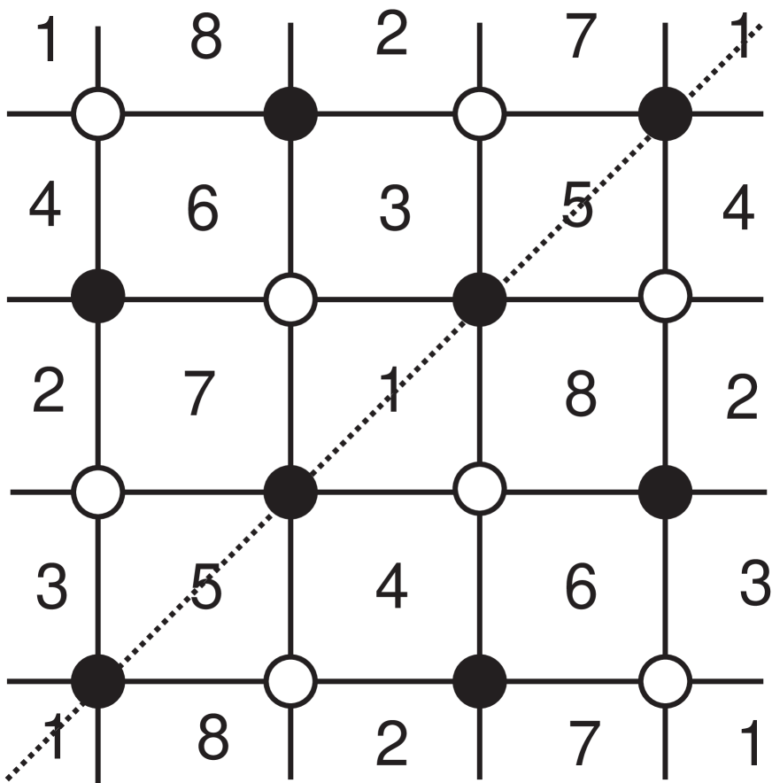
Figure 11: Dimer graph/brane box picture for a toric degeneration of Del Pezzo 5.

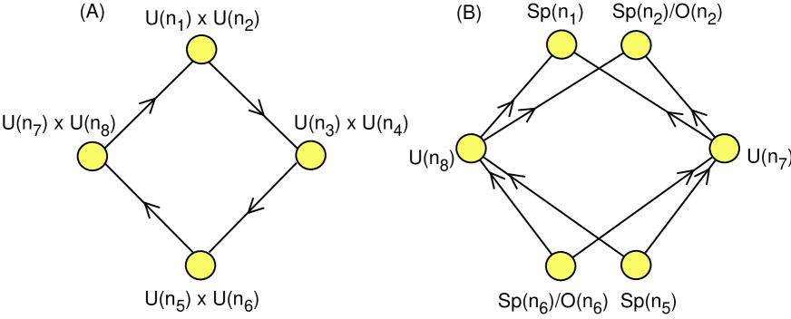
Figure 12: (A): The Del Pezzo 5 quiver. (B): Orientifold associated to the toric $Z_{2}$ symmetry.

We are interested in the following orientifold action:

$$1\leftrightarrow 1^{*},\quad 2\leftrightarrow 2^{*},\quad 3\leftrightarrow 8^{*},\quad 4\leftrightarrow 7^{*},\quad 5\leftrightarrow 5^{*},\quad 6\leftrightarrow 6^{*}.$$ (3.18)

The action on the fields is

$$\begin{array}[]{cccc}X_{13}^{T}\gamma_{1}=X_{81}&X_{14}^{T}\gamma_{1}=a\,X_{71}&X_{23}^{T}\gamma_{2}=bX_{82}&X_{24}^{T}\gamma_{2}=X_{72}\\ \gamma_{5}^{-1}X_{35}^{T}=X_{58}&\gamma_{5}^{-1}X_{45}^{T}=X_{57}&\gamma_{6}^{-1}X_{36}^{T}=X_{68}&\gamma_{6}^{-1}X_{46}^{T}=X_{67}\end{array}$$ (3.19)

where $a$ and $b$ are phases. If we insist on taking the toric superpotential, then invariance of the superpotential implies

$$s(1)s(5)=s(1)s(6)a=s(1)s(6)a^{-1}=s(2)s(5)b^{-1}=s(2)s(5)b=s(2)s(6)=1$$ (3.20)

Hence with this superpotential, the projections on nodes 1 and 5, and the projections on nodes 2 and 6 are always the same, but other than that it is free to be chosen. In particular the all $Sp$ projection that we will use for our first construction is actually realized in the toric limit, and can be seen for instance in the dimer description. However we will consider generic superpotentials compatible with the projection.

The orientifold locus should consist of the union of four O7-planes, coinciding with the fractional branes of nodes $1,2,5$ and $6$.

Another orientifold of Del Pezzo 5

We consider the same Del Pezzo 5 quiver, but with an alternative orientifold action

$$1\to 1^{*},\qquad 2\to 2^{*},\qquad 3\to 8^{*},\qquad 4\to 7^{*},\qquad 5\to 6^{*}.$$ (3.21)

The conditions on the fields are

$$X_{13}^{T}\gamma_{1}=X_{81},X_{14}^{T}\gamma_{2}=X_{71},X_{23}^{T}\gamma_{2}=X_{82},X_{24}^{T}\gamma_{2}=X_{72},$$ (3.22)

$$X_{35}^{T}=X_{68},X_{36}^{T}=X_{58},X_{45}^{T}=X_{67},X_{46}^{T}=X_{57}.$$ (3.23)

We take the $Sp/Sp$ projection on nodes 1 and 2. Presumably there are two O7-planes, coinciding with the fractional branes on nodes $1$ and $2$.

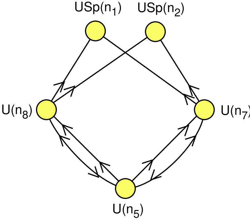
Figure 13: Another interesting orientifold of Del Pezzo 5.

Del Pezzo 7

Several other Del Pezzo quivers could be used for MSSM constructions. We briefly mention a quiver for Del Pezzo 7. The vanishing homology classes again consist of the class of the 4-cycle, 0-cycle, the hyperplane class $H$, and the exceptional curves $E_{i},i=1,\ldots,7$, with the intersection numbers

$$H\cdot H=1,\quad H\cdot E_{i}=0,\quad E_{i}\cdot E_{j}=-\delta_{ij}.$$ (3.24)

An exceptional collection is given by

$$\begin{array}[]{llll}1.\ \ (2,H,-\frac{1}{2})&2.\ -(1,H\!-\!E_{5},0)\\ &3.\ -(1,H\!-\!E_{6},0)\\ &4.\ -(1,H\!-\!E_{7},0)\\ &5.\ -(1,3H\!-\!\sum_{i}E_{i},1)\\ &\\ 6.\ -(2,E_{5}\!+\!E_{6}\!+\!E_{7},-{3\over 2})&7.\ \ (1,H\!-\!E_{1},0)\\ &8.\ \ (1,H\!-\!E_{2},0)\\ &9.\ \ (1,H\!-\!E_{3},0)\\ &10.\,(1,H\!-\!E_{4},0)\\ \end{array}$$ (3.25)

One way to orientifold this quiver is by reflecting in the axis through nodes $1$ and $6$.

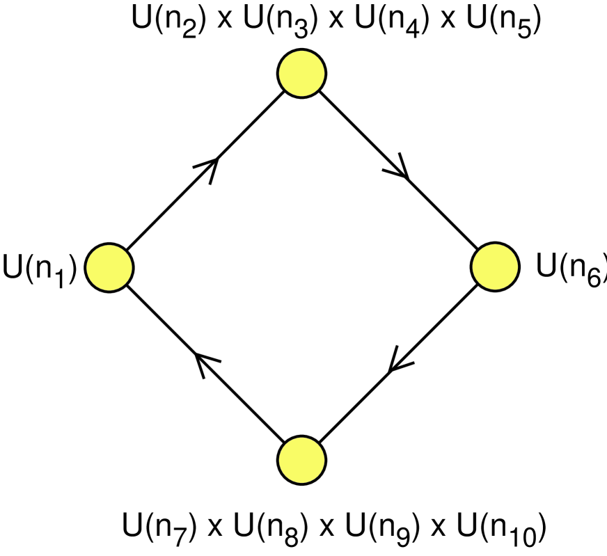
Figure 14: Quiver for Del Pezzo 7.

4. The Higgsing procedure

4.1. Model I

Now we would like to engineer the MSSM quivers we have discussed. We take the quiver in figure 12 with an $Sp/Sp/Sp/Sp$ projection. As far as the chiral field content goes, this contains the MSSM with one generation of quarks and leptons. In order to increase the number of generations, we have to create some non-trivial bound states of fractional branes.

Let us try to give a rather imprecise but intuitive geometric picture of our procedure (which we will then promptly abandon in favour of more precise statements). Each fractional brane corresponds to a line bundle on the Del Pezzo surface, i.e. a non-trivial $U(1)$ gauge field configuration. Roughly we want to take three identical fractional branes (which corresponds to a $U(1)^{3}$ field configuration with $U(1)$ holonomy) and add some instantons to get a field configuration with $U(3)$ holonomy on the Del Pezzo. Recall that the 4D gauge symmetry is the subgroup of the gauge group on the brane that commutes with the holonomy. This new fractional brane then has the same intersection numbers as the original brane, times a factor of three. Any moduli of the new fractional brane can be lifted by turning on suitable $B$-fields.

The more pedestrian and precise statements are that we first increase the ranks of the gauge groups and then turn on suitable VEVs in order to get to the quiver we want. We claim that there exists a bound state $F_{b}$ with the following charge vector:

$${\rm ch}(F_{b}) = \sum_{i}n_{i}\,{\rm ch}(F_{i})=-(3,2H\!-\!E_{2}\!-\!E_{3}\!+\!E_{4}\!+\!E_{5},-2),$$

$$\vec{n} = \{1,0,1,1,2,2,1,1\}.$$ (4.1)

To see this, let’s fix the gamma matrices to be

$$\gamma_{1}=i\sigma_{2}=\left(\begin{array}[]{cc}0&1\\ -1&0\\ \end{array}\right),\quad\gamma_{5}=\gamma_{6}=\left(\begin{array}[]{cc}i\sigma_{2}&0\\ 0&i\sigma_{2}\\ \end{array}\right),$$ (4.2)

and consider the following VEVs:

$$X_{13}=\left(\begin{array}[]{c}b_{1}\\ \end{array}\right)\!,\ X_{35}=\left(\begin{array}[]{cc}b_{2}&0\\ \end{array}\right)\!,\ X_{36}=\left(\begin{array}[]{cc}b_{3}&0\\ \end{array}\right)\!,$$ (4.3)

$$X_{14}=\left(\begin{array}[]{c}d_{1}\\ \end{array}\right)\!,\ X_{45}=\left(\begin{array}[]{cc}0&d_{2}\\ \end{array}\right)\!,\ X_{46}=\left(\begin{array}[]{cc}0&d_{3}\\ \end{array}\right)\!,$$ (4.4)

with the remaining fields determined by the orientifold conditions. The entries here are $2\times 2$ matrices. These VEVs break the gauge symmetry to $Sp(2)$, so the fractional brane $F_{b}$ will come with an $Sp$-projection. The D-term equations may be satisfied by taking

$${1\over 5}b_{1}={1\over 4}b_{2}={1\over 3}b_{3}=\left(\begin{array}[]{cc}\chi_{1}&0\\ 0&\chi_{1}\\ \end{array}\right),\qquad{1\over 5}d_{1}={1\over 4}d_{2}={1\over 3}d_{3}=\left(\begin{array}[]{cc}\chi_{2}&0\\ 0&\chi_{2}\\ \end{array}\right).$$ (4.5)

Clearly we need both quartic and octic terms in the superpotential, in order to get mass terms for the adjoints associated with a rescaling of the VEVs. With such a superpotential, tuned so that the F-term equations are satisfied and so that the orientifold symmetry is preserved, but otherwise generic, we find that our bound state is rigid, i.e. it has no massless adjoints.

We also claim that there exists a bound state $F_{a}$ with the following charge vector:

$${\rm ch}(F_{a}) = \sum_{i}n_{i}\,{\rm ch}(F_{i})=(3,2H\!-\!E_{1}\!-\!E_{2}\!+\!E_{4}\!+\!E_{5},0),$$

$$\vec{n} = \{2,2,1,1,1,0,1,1\}$$ (4.6)

This is very similar to $F_{b}$ so we do not need to repeat the analysis. The fractional brane $F_{a}$ also inherits an $Sp$ projection.

Next we compute the massless fields in the quiver for $\{2F_{a},3F_{3},F_{4},2F_{b},F_{7},3F_{8}\}$. For a generic superpotential (apart from the conditions mentioned above) we found that the spectrum is completely chiral, as shown in figure 15. This quiver is a Higgsed version of the original Del Pezzo quiver. It inherits the following orientifold projection:

$$X^{iT}_{a3}\gamma_{a}=X^{i}_{8a},\quad X_{a4}^{iT}\gamma_{a}=X_{7a}^{i},\quad\gamma_{b}^{-1}X_{3b}^{iT}=X^{i}_{b8},\quad\gamma_{b}^{-1}X_{4b}^{iT}=X^{i}_{b7},\quad i=1,2,3.$$ (4.7)

Moreover, we expect to be able to get a generic superpotential for this quiver provided we included sufficiently many higher order terms in the original Del Pezzo quiver. Checking we can get generic 4th and 8th order terms is computationally too intensive, so we will assume it from now on.

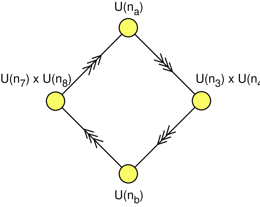
Figure 15: Intermediate quiver.

This is almost what we want. After orientifolding we get all the chiral fields of the MSSM. However, we also want some non-chiral matter: the conventional Higgses $H_{u},H_{d}$ and the additional Higgs fields which break $Sp(2)_{R}\times U(1)_{L}\to U(1)$. This cannot be obtained by tuning the original bound state/superpotential, because the candidate non-chiral fields are in fact eaten by gauge bosons. So we create a new quiver with the same chiral matter content, but with more candidate non-chiral fields. To do this we replace $F_{b}$ by the bound state $F_{d}$ with charge vector

$${\rm ch}(F_{d}) = {\rm ch}(F_{a})+{\rm ch}(F_{3})+2\,{\rm ch}(F_{b})+{\rm ch}(F_{8})$$ (4.8)

$$= -(3,2H+E_{1}-E_{2}-E_{3}+E_{5},-4)$$

This can be done for instance by turning on VEVs of the following form:

$$X_{a4}^{1}=\left(\begin{array}[]{c}s_{1}\\ \end{array}\right)\quad X_{4b}^{1}=\left(\begin{array}[]{cc}s_{2}&0\\ \end{array}\right)\quad X_{4b}^{2}=\left(\begin{array}[]{cc}0&s_{3}\\ \end{array}\right)$$ (4.9)

and the remaining non-zero VEVs fixed by the orientifold conditions. We can satisfy the D-terms by setting

$${1\over 5}s_{1}={1\over 4}s_{2}={1\over 3}s_{3}=\left(\begin{array}[]{cc}\phi&0\\ 0&\phi\\ \end{array}\right).$$ (4.10)

In order for this to satisfy the F-term equations, and to get the desired massless non-chiral matter, we have to impose some restrictions on the superpotential. If we use both quartic and octic terms, one can lift all the non-chiral matter and the quiver generated by $\{2F_{a},3F_{3},F_{4},2F_{d},F_{7},3F_{8}\}$ is the same as in figure 15 again. However now there are two non-chiral pairs between $F_{a}$ and $F_{d}$ and two non-chiral pairs between $F_{d}$ and $F_{4}/F_{7}$. We have checked that the superpotential can be tuned so that one of each of these pairs becomes light, and so we end up with the required quiver in figure 6A.

4.2. Pati-Salam

The quiver we have obtained above also gives a three generation SUSY Pati-Salam model, by changing the ranks of the gauge groups ($U(3)\to U(0)$, and $U(1)\to U(4)$).

Very similar tricks may also be applied to the ${\bf P}^{1}\times{\bf P}^{1}$ quiver to construct Pati-Salam models, though in that case the number of generations will be even. Let us show how we can obtain a four generation Pati-Salam model. We define the gamma matrices as

$$\gamma_{1}=\left(\begin{array}[]{cc}0&1\\ -1&0\\ \end{array}\right),\qquad\gamma_{3}=\left(\begin{array}[]{cc}0&{\bf 1}_{3\times 3}\\ -{\bf 1}_{3\times 3}&0\\ \end{array}\right),$$ (4.11)

Then we construct a bound state $F_{b}$ with charge vector

$${\rm ch}(F_{b})={\rm ch}(F_{1})+2{\rm ch}(F_{2})+3{\rm ch}(F_{3})+2{\rm ch}(F_{4})=-(2,H_{2}\!-\!H_{1},3)$$ (4.12)

by turning on the following VEVs:

$$X_{12}=\left(\begin{array}[]{cccc}a_{1}&0&0&0\\ 0&0&a_{1}&0\\ \end{array}\right),\quad Y_{12}=\left(\begin{array}[]{cccc}0&a_{1}&0&0\\ 0&0&0&a_{1}\\ \end{array}\right)\quad,$$ (4.13)

$$X_{23}=\left(\begin{array}[]{cccccc}a_{2}&0&0&0&0&0\\ 0&0&a_{3}&0&0&0\\ 0&0&0&a_{2}&0&0\\ 0&0&0&0&0&a_{3}\\ \end{array}\right),\quad Y_{23}=\left(\begin{array}[]{cccccc}0&0&0&0&0&0\\ 0&a_{4}&0&0&0&0\\ 0&0&0&0&0&0\\ 0&0&0&0&a_{4}&0\\ \end{array}\right)$$ (4.14)

with the remaining VEVs determined by the orientifold symmetry. The D-terms are satisfied if we pick

$$a_{1}=a_{2}=5\psi,\quad a_{3}=4\psi,\quad a_{4}=3\psi.$$ (4.15)

Similarly we construct a bound state $F_{a}$ with charge vector

$${\rm ch}(F_{a})=3{\rm ch}(F_{1})+2{\rm ch}(F_{2})+{\rm ch}(F_{3})+2{\rm ch}(F_{4})=(2,H_{2}\!-\!H_{1},-1).$$ (4.16)

Then by orientifolding the quiver generated by $\{2F_{a},4F_{2},2F_{b},4F_{4}\}$ we get the Pati-Salam quiver with four generations in figure 16. It’s expected all excess non-chiral matter can be lifted by an induced superpotential, but we did not try very hard to do it explicitly in this case. The total configuration has net wrapping number $(0,4H_{2}-4H_{1},-8)$.

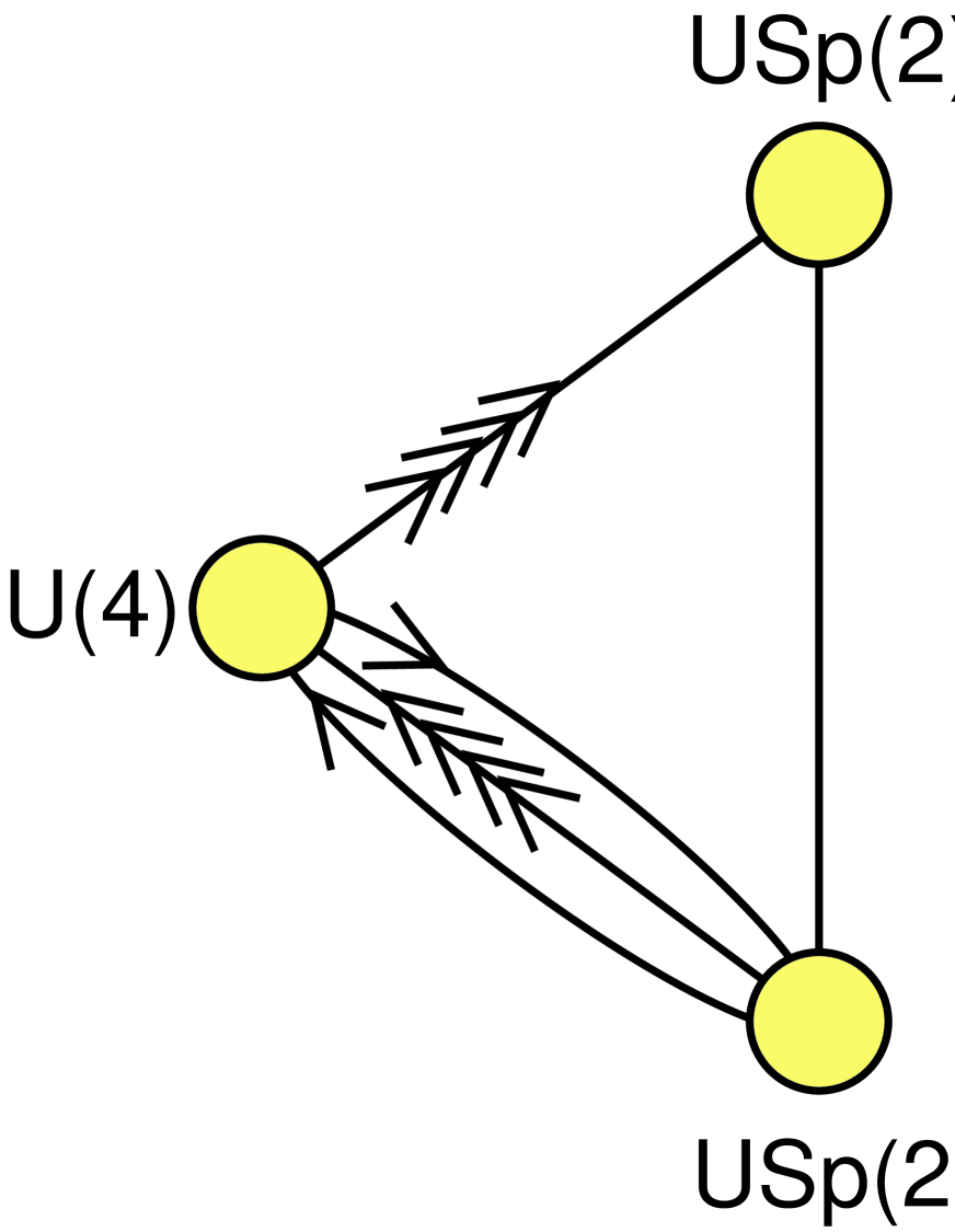
Figure 16: A four generation Pati-Salam model from ${\bf P}^{1}\times{\bf P}^{1}$.

4.3. Model II

We now consider an alternative construction, in which $U(1)_{B-L}$ can get a mass through the Stückelberg mechanism (depending on the UV completion [32]).

The orientifold projection is as in (3.21). We would like to form the following bound states:

$${\rm ch}(F_{a}) = \sum_{i}n_{i}\,{\rm ch}(F_{i})=(3,2H\!-\!2E_{1}\!+\!E_{2}\!-\!E_{3}\!+\!E_{4}\!+\!E_{5},1),$$

$$\vec{n}_{a} = \{4,1,2,2,1,1,2,2\}$$

$${\rm ch}(F_{b}) = \sum_{i}n_{i}\,{\rm ch}(F_{i})=-(3,\!-\!E_{1}\!-\!2E_{2}\!+\!3E_{3}\!+\!3E_{4}\!+\!3E_{5},6),$$

$$\vec{n}_{b} = \{2,1,3,3,0,6,3,3\}$$

$${\rm ch}(F_{b^{\prime}}) = \sum_{i}n_{i}\,{\rm ch}(F_{i})=-(3,6H\!-\!E_{1}\!-\!2E_{2}\!-\!3E_{3}\!-\!3E_{4}\!-\!3E_{5},0),$$

$$\vec{n}_{b^{\prime}} = \{2,1,3,3,6,0,3,3\}$$ (4.17)

For $2F_{a}$ we suggest the following VEVs:

$$X_{13}=\left(\begin{array}[]{cccc}a_{1}&0&0&0\\ 0&a_{2}&0&0\\ 0&0&0&0\\ 0&0&0&0\\ 0&0&a_{1}&0\\ 0&0&0&a_{2}\\ 0&0&0&0\\ 0&0&0&0\\ \end{array}\right),\quad X_{14}=\left(\begin{array}[]{cccc}0&0&0&0\\ 0&0&0&0\\ a_{2}&0&0&0\\ 0&a_{1}&0&0\\ 0&0&0&0\\ 0&0&0&0\\ 0&0&a_{2}&0\\ 0&0&0&a_{1}\\ \end{array}\right),$$ (4.18)

$$X_{23}=\left(\begin{array}[]{cccc}a_{3}&0&0&0\\ 0&0&a_{3}&0\\ \end{array}\right),\quad X_{24}=\left(\begin{array}[]{cccc}0&a_{3}&0&0\\ 0&0&0&a_{3}\\ \end{array}\right),$$ (4.19)

$$X_{35}=\left(\begin{array}[]{cc}a_{4}&0\\ 0&0\\ 0&a_{4}\\ 0&0\\ \end{array}\right),\quad X_{36}=\left(\begin{array}[]{cc}0&0\\ 0&a_{5}\\ 0&0\\ a_{5}&0\\ \end{array}\right),\quad X_{45}=\left(\begin{array}[]{cc}0&0\\ a_{5}&0\\ 0&0\\ 0&a_{5}\\ \end{array}\right),\quad X_{46}=\left(\begin{array}[]{cc}a_{4}&0\\ 0&0\\ 0&a_{4}\\ 0&0\\ \end{array}\right).$$ (4.20)

The remaining fields are determined by the orientifold conditions (3.22). We took the gamma matrices to be

$$\gamma_{1}=\left(\begin{array}[]{cc}0&{\bf 1}_{4\times 4}\\ -{\bf 1}_{4\times 4}&0\\ \end{array}\right),\qquad\gamma_{2}=\left(\begin{array}[]{cc}0&1\\ -1&0\\ \end{array}\right).$$ (4.21)

The D-term equations reduce to

$$|a_{1}|^{2}+|a_{3}|^{2}=|a_{4}|^{2},\quad|a_{2}|^{2}=|a_{5}|^{2}$$ (4.22)

which is easily satisfied. By computing the gauge generators that are preserved, one can check that this bound state indeed inherits an $Sp$-projection.

For $F_{b}+F_{b^{\prime}}$ we consider the following VEVs:

$$X_{13}=X_{14}=\left(\begin{array}[]{cccccc}e_{1}&0&0&0&0&0\\ 0&e_{1}&0&0&0&0\\ 0&0&0&e_{1}&0&0\\ 0&0&0&0&e_{1}&0\\ \end{array}\right),\quad X_{23}=X_{24}=\left(\begin{array}[]{cccccc}0&0&e_{1}&0&0&0\\ 0&0&0&0&0&e_{1}\\ \end{array}\right),$$ (4.23)

$$\quad X_{35}=\left(\begin{array}[]{cccccc}e_{1}&0&0&0&0&0\\ 0&e_{1}&0&0&0&0\\ 0&0&e_{1}&0&0&0\\ 0&0&0&0&0&0\\ 0&0&0&0&0&0\\ 0&0&0&0&0&0\\ \end{array}\right),\quad X_{45}=\left(\begin{array}[]{cccccc}0&0&0&e_{1}&0&0\\ 0&0&0&0&e_{1}&0\\ 0&0&0&0&0&e_{1}\\ 0&0&0&0&0&0\\ 0&0&0&0&0&0\\ 0&0&0&0&0&0\\ \end{array}\right),$$ (4.24)

$$\quad X_{36}=\left(\begin{array}[]{cccccc}0&0&0&0&0&0\\ 0&0&0&0&0&0\\ 0&0&0&0&0&0\\ 0&0&0&0&0&e_{1}\\ 0&0&0&e_{1}&0&0\\ 0&0&0&0&e_{1}&0\\ \end{array}\right),\quad X_{46}=\left(\begin{array}[]{cccccc}0&0&0&0&0&0\\ 0&0&0&0&0&0\\ 0&0&0&0&0&0\\ 0&0&e_{1}&0&0&0\\ e_{1}&0&0&0&0&0\\ 0&e_{1}&0&0&0&0\\ \end{array}\right),$$ (4.25)

with the remaining VEVs determined by (3.22). Here we took the gamma matrices to be

$$\gamma_{1}=\left(\begin{array}[]{cc}0&{\bf 1}_{2\times 2}\\ -{\bf 1}_{2\times 2}&0\\ \end{array}\right),\qquad\gamma_{2}=\left(\begin{array}[]{cc}0&1\\ -1&0\\ \end{array}\right).$$ (4.26)

The D-terms are satisfied. Note that we have used the notation $F_{b}+F_{b^{\prime}}$ to indicate that this representation has two unbroken $U(1)$’s. They get mapped into each other under the orientifolding.

After orientifolding the quiver generated by $\{2F_{a},3F_{3},F_{4},F_{b}+F_{b^{\prime}},F_{7},3F_{8}\}$ we get a quiver with the expected chiral matter content of the MSSM, with three generations, and Higgs fields. These are some of the most complicated bound states in this paper, and we have not been able to check that all excess non-chiral matter can be lifted by an induced superpotential.

We can also argue that all the remaining $U(1)$’s couple to an independent Stückelberg field. This is not automatically true but can be checked in this case. To see this, before Higgsing and orientifolding the Stückelberg couplings are of the form

$$\sum_{\rm{nodes}\ i}\int C^{(i)}\wedge{\rm Tr}(F_{(i)}),$$ (4.27)

where $C^{(i)},F_{(i)}$ are the Stückelberg 2-form field and gauge field for the $i$th node. After Higgsing we get

$$\sum_{i,j}n_{i}^{j}\ \int C^{(i)}\wedge{\rm Tr}({\tilde{F}}_{(j)})$$ (4.28)

where $n_{i}^{j}$ is the number of original fractional branes of type $i$ contained in the bound state $j$, $j\in\{a,3,4,b,b^{\prime},7,8\}$, and ${\tilde{F}}_{(j)}$ is the corresponding gauge field. Now it is easy to check that for our MSSM configuration the rank of $n_{i}^{j}$ is maximal, so that all the $U(1)$’s couple to an independent Stückelberg field. We conclude that the $U(1)_{B-L}$ gauge boson can be lifted through the Stückelberg mechanism.

5. Dynamical SUSY breaking

Since Del Pezzo quivers are chiral, one may expect to find examples of local models with dynamical supersymmetry breaking. However it was typically found in examples that if SUSY breaking occurred there was some runaway mode which invalidated the model [33, 34, 35, 36, 37]. Some effort has gone in to finding a way to stabilise such runaway modes [38, 39, 40].

We have seen that orientifolding eliminates Kähler moduli, so one may revisit this issue by looking for simple models where the runaway mode is projected out. In fact the new techniques allow us to engineer many familiar models which are known to break SUSY dynamically. Examples include:

5.1. A non-calculable model

Let us consider the ${\bf C}^{3}/Z_{3}\times Z_{3}$ orbifold. This is the Calabi-Yau three-fold defined by the equation

$$xyz=t^{3},$$ (5.1)

i.e. it is a cone over a DP6 surface which itself has three $A_{2}$ singularities. The quiver in shown in figure 17A. For completeness, let us also mention an exceptional collection:

$$\begin{array}[]{lll}1.\ (1,E_{4},-\frac{1}{2})&4.\ -(2,H,-\frac{1}{2})&7.\ (1,H\!-\!E_{1},0)\\ 2.\ (1,E_{5},-\frac{1}{2})&5.\ -(2,2H\!-\!E_{1}\!-\!E_{2}\!-\!E_{3},-\frac{1}{2})&8.\ (1,H\!-\!E_{2},0)\\ 3.\ (1,E_{6},-\frac{1}{2})&6.\ -(2,E_{4}\!+\!E_{5}\!+\!E_{6},-{3\over 2})&9.\ (1,H\!-\!E_{3},0)\\ \end{array}$$ (5.2)

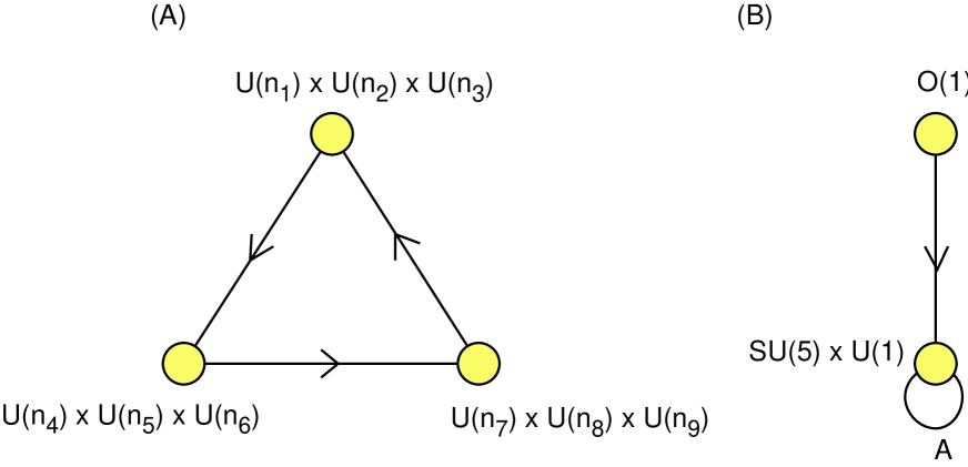
Figure 17: (A): The quiver for ${\bf C}^{3}/Z_{3}\times Z_{3}$, an orbifold limit of DP6. (B): Orientifold of a fractional brane of (A).

Now we are interested in the canonical orientifold action on the nodes, which exchanges oppositely twisted sectors :

$$1\to 1^{*},\quad 2\to 3^{*},\quad 4\to 9^{*},\quad 5\to 8^{*},\quad 6\to 7^{*}$$ (5.3)

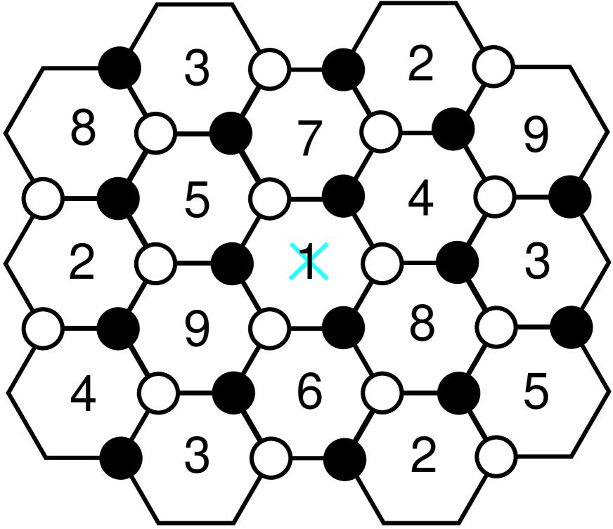
Figure 18: The dimer for the ${\bf C}^{3}/Z_{3}\times Z_{3}$ orbifold. The orientifold acts by a $180^{0}$ rotation centered at the cross.

This is a symmetry of the dimer diagram, as indicated in figure 18. Let’s take the fractional brane which only uses nodes $\{1,5,8\}$, as shown in figure 17. This is a model with two gauge groups, $U(5)$ and $O(1)=\{\pm 1\}$. The $U(1)\subset U(5)$ gets a mass through the Stückelberg mechanism, so we are left only with the $SU(5)$, with matter in the $10+\bar{5}$. Since there are no gauge invariant baryonic operators we can write down, integrating out the massive $U(1)$ leads to a D-term potential for the dynamical FI-term (a normalizable closed string mode), stabilizing it. Thus what we are left over with is precisely the model considered by [41]. This model has no classical flat directions and a non-anomalous R-symmetry that was argued to be broken, and therefore supersymmetry is broken dynamically.

An important property of this gauge theory is that it has very few parameters, so there is little room for a runaway of the parameters after coupling to 4D gravity. Moreover coming from such a simple singularity, the model should not be so hard to embed in a compact CY. For instance, we can easily embed the singularity in the quintic, by taking an equation of the form

$$0=s^{2}(xyz-t^{3})+x^{5}+x^{4}s+\ldots$$ (5.4)

or we could try to use $T^{6}/Z_{3}\times Z_{3}$. To complete the analysis we would need to check that the orientifold can be extended globally and tadpoles can be cancelled.

It would be nice to see the supersymmetry breaking from a dual gravity perspective. There is presumably an enhançon type of effect at work, similar to [43, 44].

5.2. The 3-2 Model

Our next model is a little harder to produce, so we start by drawing the quiver diagram in figure 19A, and its oriented cover in figure 19B.

Figure 19: (A): The 3-2 model, with an extra massive $U(1)$. (B): Oriented cover of the quiver in (A).

This is known as the 3-2 model [45]. The stringy version has an additional anomalous $U(1)$, which does not affect the low energy dynamics as in the previous example. There are various large $N$ generalizations which appear to have no classical flat directions and a spontaneously broken R-symmetry, and so should also break supersymmetry.

The covering quiver has a certain similarity with DP5. So we take the DP5 quiver with the projections (3.19) and $a=b=-1$, with $Sp$-projections on nodes 1 and 5, and $SO$-projections on nodes 2 and 6. We take

$$\gamma_{2}={\bf 1}_{3\times 3},\quad\gamma_{6}={\bf 1}_{5\times 5}$$ (5.5)

and consider a bound state $F_{a}$ with charge vector

$${\rm ch}(F_{a})=\sum_{i}n_{i}\,{\rm ch}(F_{i}),\qquad\vec{n}=\{0,3,2,3,0,5,3,2\}.$$ (5.6)

Concretely, the VEVs are given by

$$X_{23}=\left(\begin{array}[]{cc}a_{1}&0\\ 0&a_{2}\\ 0&0\\ \end{array}\right),\quad X_{24}=\left(\begin{array}[]{ccc}a_{1}&0&0\\ 0&a_{2}&0\\ 0&0&a_{2}\\ \end{array}\right),$$ (5.7)

$$X_{36}=\left(\begin{array}[]{ccccc}a_{3}&0&a_{4}&0&a_{5}\\ 0&a_{6}&0&a_{7}&0\\ \end{array}\right),\quad X_{46}=\left(\begin{array}[]{ccccc}0&a_{8}&0&0&0\\ 0&0&a_{9}&0&0\\ 0&0&0&0&a_{10}\\ \end{array}\right),$$ (5.8)

with the remaining VEVs either zero or determined by (3.19). The D-terms then imply

$$|a_{1}|^{2}=|a_{3}|^{2}+|a_{4}|^{2}+|a_{5}|^{2}=|a_{8}|^{2},\quad|a_{2}|^{2}=|a_{6}|^{2}+|a_{7}|^{2}=|a_{9}|^{2}=|a_{10}|^{2}$$ (5.9)

which is easily satisfied.

The quiver generated by $\{2\,F_{1},3\,F_{3},F_{a},3\,F_{8}\}$ is of the required form in figure 19, up to non-chiral matter. The lepton doublets can get masses only in pairs. Our orientifolded quiver has five lepton doublets, and in principle we may turn on mass terms for four of them, leaving one massless.

5.3. ISS meta-stable models

A number of realizations of ISS vacua [46] from quivers have already been considered [47, 48]. We would like to suggest an alternative realization, in which the quark masses are obtained in a more straightforward way.

As we discussed in section 2 we can take the conifold quiver and turn on mass terms:

$$W=m_{ij}\,{\rm Tr}(A^{i}B^{j})+\lambda\,{\rm Tr}(A^{1}B^{1}A^{2}B^{2}-A^{1}B^{2}A^{2}B^{1})$$ (5.10)

We introduce the dimensionless parameters $a=m/E,b=\lambda E$ and consider the regime $a>>b$ so that we can ignore the quartic term. The non-trivial $U(1)$ gauge group is taken to decouple from the low energy physics, either by working on the infinite cone or by coupling to a Stückelberg field in compactified settings. We also set the gauge coupling of $SU(n_{2})$ to be very weak. Finally we take $n_{1}/2<n_{2}<3n_{1}/4$. Then the $SU(n_{1})$ flows to strong coupling and we apply a Seiberg duality. The dual theory has gauge group $SU(2n_{2}-n_{1})\times SU(n_{2})$, with two pairs of bifundamentals of opposite charges, and four adjoints for $SU(n_{2})$. In particular both gauge groups are now IR free.

Thus now we are in the situation of ISS, except that we have gauged a slightly different subgroup of the global symmetry group when the gauge coupling for $SU(n_{2})$ is finite. In this theory SUSY is broken by the rank condition, and there are meta-stable vacua for zero adjoint VEVs with pseudomoduli lifted by a one-loop potential. Actually if we would have kept the quartic terms of the conifold quiver then we get mass terms for the mesons and we can solve the F-terms, but because we took $a>>b$ these SUSY vacua are very far out in meson field space and don’t affect the analysis near the origin.

In the meta-stable vacua, the gauge group $SU(2n_{2}-n_{1})\times SU(n_{2})$ is broken to $SU(2n_{2}-n_{1})\times SU(n_{1}-n_{2})$. If the $SU(n_{2})$ gauge coupling is small enough, then both the gauge couplings of the remaining $SU(2n_{2}-n_{1})\times SU(n_{1}-n_{2})$ are also very small. There are also some massless Goldstone bosons left from the broken global symmetries, and some light fermions. The Goldstone bosons parametrize a compact coset $G/H$ and are not charged under the remaining gauge groups. Thus the remaining gauge groups may eventually become strong in the deep IR and generate some vacuum energy. But since the strong coupling scale is arbitrarily small, this means there must still be long-lived meta-stable vacua close to those found by ISS.

6. Topological criteria for unification

From the bottom-up perspective, there is no a priori relation between the MSSM couplings. For instance the differences between the (inverse squared) gauge couplings depend on complexified Kähler moduli. If such moduli extend to the UV completion, we will have to find a suitable potential to stabilize them, and it seems there is no natural reason to expect any relation between them.

On the other hand we clearly do not live at a random point on the parameter space. There are many relations among the couplings that we believe to be a reflection of new physics. So one may ask if these relations have a special significance in our set-up.

Recently it has been argued that moduli corresponding to non-normalizable closed string modes may be trivializable, in the sense that they appear to exist locally but may not be extended to the UV completion [32]. (A similar scheme for the 6-volume was proposed in [49]). This is really a rephrasing of the obvious fact that the most interesting UV completions are those which are as rigid as possible, consistent with observed low energy physics, because they give a topological explanation of the tree level relations between certain couplings, as opposed to a dynamical one due to moduli stabilisation. It also reduces the number of global tadpoles to be cancelled.

Let us review some aspects of this trivialization for Kähler moduli. Suppose that two fractional branes wrap vanishing cycles $a$ and $b$, giving rise to a gauge group $U(n_{a})\times U(n_{b})$, embedded in some orientifold compactification. Locally the homology class $a-b$ has an even lift and an odd lift, where even and odd refer to the eigenvalue of the homology classes under the orientifold action. Let us further assume that $a-b$ is the class of a 2-cycle that does not intersect a vanishing 4-cycle. Then if the odd lift is trivializable, we have the tree level relation

$${4\pi\over g_{a}^{2}}-i{\vartheta_{a}\over 2\pi}={4\pi\over g_{b}^{2}}-i{\vartheta_{b}\over 2\pi}$$ (6.1)

and if the even lift is trivializable we have

$$\zeta_{a}+ic_{a}=\zeta_{b}+ic_{b}$$ (6.2)

where $\zeta$ couples as an FI-term and $c$ is its axion partner. A certain linear relation between the axions is needed to keep hypercharge massless.

Now suppose for ease of discussion that both lifts are trivializable, so that $a$ and $b$ are the same cycle homologically. We can model this by considering a single fractional brane with an adjoint scalar field whose superpotential has two critical points. Thus morally the vacuum where the two branes sit apart is a Higgsed vacuum of a unified theory with gauge group $U(n_{a}+n_{b})$, in particular the tree level gauge couplings of $U(n_{a})$ and $U(n_{b})$ are related as above. Integrating out the massive adjoint we generate certain higher order superpotential couplings suppressed by the mass of the adjoint field, which should correspond to the subleading complex structure deformations discussed in [32].

This also explains the origin of the monopoles discovered in [50]: they are D-branes stretched between the gauge branes, i.e. they are the monopoles in the Higgsed phase expected by a Pati-Salam like unification in the model of [2]. The unified model is actually one of the standard quivers for ${\bf P}^{2}$, with gauge group $U(4)\times U(2)\times U(2)$ and $(3,6,3)$ arrows between them.

Let us discuss how these ideas can be applied to the MSSM models that we have constructed from Del Pezzo 5. For the quivers and labelling of the nodes we refer to the figures in section 1.2. The moduli controlling the difference between the gauge couplings of $U(3)$ node and the $U(1)_{L}$ node are trivialisable, so we can give a topological explanation of the relation $g_{3}^{-2}=g_{1}^{-2}$. We can achieve this by making sure that $E_{4}-E_{5}$ or $H-E_{1}-E_{2}-E_{3}$ is globally trivial. If we assume that both are globally trivial, then we can morally think of the $U(3)$ and $U(1)$ as being unified in the Pati-Salam group $U(4)$ (i.e. we have baryon-lepton unification). In fact with only a small change in interpretation this situation was already proposed in [51, 52].

The further relations $g_{2}=g_{0}=g_{3}$ look quite natural because they corresponds to the branes having equal tension, and they also give precisely the standard tree level relations from $SU(5)$ unification for the strong, weak and hypercharge couplings [51]. But they cannot be imposed by topological means, because the intersection numbers of the corresponding cycles are different. However we can do the following. The tree level gauge coupling $g_{3}$ corresponds to

$${2\over g_{3}^{2}}={N\over g_{s}\ell_{s}^{2}}\int_{\alpha}B_{2},\qquad\alpha=E_{4}-E_{3}$$ (6.3)

which is a non-normalizable mode in the local geometry. Here $N$ is a numerical factor which depends on the periodicity of $B_{2}$. Similarly

$${1\over g_{2}^{2}}+{1\over g_{0}^{2}}={N\over g_{s}\ell_{s}^{2}}\int_{\beta}B_{2}$$ (6.4)

is a non-normalizable mode, where $\beta$ is some degree zero linear combination of the 2-cycles which depends on how we exactly constructed the bound states. So any linear combination of these quantities is the integral of the $B$-field over some degree zero homology class, and therefore potentially trivializable. Together with $g_{3}=g_{1}$ this then leads to a tree level relation between the observed gauge couplings

$${1\over g_{Y}^{2}}+{1\over g_{W}^{2}}=\left[{2n_{1}\over n_{2}}+{2\over 3}\right]{1\over g_{S}^{2}}$$ (6.5)

where we have assumed that $n_{1}\alpha-n_{2}\beta$ is trivialized. This is compatible with the relations from $SU(5)$ unification, $g_{S}^{-2}=g_{W}^{-2}={3\over 5}g_{Y}^{-2}$ if we take $\beta=\alpha$ in homology.

Since $\int_{\alpha}B_{2}-\int_{\beta}B_{2}=\int_{\gamma}H_{3}$, where $\partial\gamma=\alpha-\beta$, one might wonder if these tree level relations are not affected if we turn on background fluxes. This seems unlikely for the following reason. As long as no background fields are turned on we should expand the $B$-field in harmonic forms and the above criterion is sufficient to guarantee that the gauge couplings are related. When we turn on general closed string deformations it is not necessarily true that the $B$-field must be expanded in harmonic forms; however it is unlikely that we gain additional zero modes and so the relation between the couplings, which is due to a lack of zero modes, should not be affected.

7. Final thoughts

It should be clear by now that the set of quiver gauge theories that can be obtained from branes at singularities is rather large. It is our impression that virtually any quiver can be constructed locally, and we believe this is really the main message of this paper. It will probably not be possible to couple every such model to 4D gravity, but given a local model it will be very hard to argue that it cannot be consistently coupled to gravity.

One would like to understand if the local D-brane scenario has something to add to discussions of beyond the SM physics. On the one hand it seems premature. After many years of work, the field theory community has not been able to come up with a single model that adresses all concerns. String phenomenology is going to have to address the same issues, and barring a miraculous discovery of the correct UV completion it would be naive to expect that doing string phenomenology would magically improve on this situation. On the other hand, string phenomenology has traditionally been more a source of new ideas and intuition than a source of accurate models.

One way to proceed is to try and isolate desirable features and translate them into geometrical or even topological terms. We have already discussed a topological explanation for tree level relations between gauge couplings. Other important issues are flavour problems. For instance we would like to explain hierarchies among the Yukawa couplings, and we would like to explain why new physics doesn’t generate large FCNC’s. Can we translate these criteria into geometric terms, and perhaps guarantee them through topological mechanisms similar to section 6? Such rigidity requirements may eliminate the majority of UV completions in the string landscape.

Another important criterion will be stability. The apparent long-lived nature of our universe suggests we are in a vacuum which does not have too many vacua in its neighbourhood with a large cumulative probability to decay away to. This makes stability a very acute issue with possible predictive power, and we might expect string theory to have something to say about this.

The bottom-up perspective also allows us to take a step back and see if top-down approaches could benefit from new ingredients. It seems that non-commutative internal geometries play an important role. Thus perhaps we should be paying more attention to backgrounds of the type recently constructed in [54].

7.1. On soft SUSY breaking

In this paper we have repeatedly used the technique of deforming the gauge theory to get rid off undesirable particles. By the same logic we can proceed to turn on masses for all the superpartners of the Standard Model fields and recover the non-SUSY Standard Model itself. This must be possible, but it is not terribly helpful. Although the dictionary between the local geometry and the superpotential deformations used in this paper are fairly well understood and can in principle be solved exactly, unfortunately the dictionary for SUSY breaking deformations is more complicated. It requires understanding Kaehler deformations which can probably only be addressed numerically, and it requires further generalizing the notion of geometry in ways that are probably not yet quite understood. Even for simpler theories like $N=4$ Yang-Mills, little is known about the stringy description of non-supersymmetric deformations. Progress can perhaps be made if one can identify special points on the parameter space where the stringy description simplifies.

7.2. Composite Higgses?

A rather curious feature of the MSSM quiver is that, if we started without Higgs fields, we can automatically generate them through Seiberg duality on $U(3)_{c}$ or $U(1)_{L}$. For the $U(3)$ node, Seiberg duality has been considered by Matt Strassler [55], who was looking for a possible embedding into a duality cascade, and also in [56]. A problem in that case is that one needs to add extra massive matter in order to make the $SU(3)$ coupling grow strong towards the UV.

In the MSSM quivers we have an alternative: we may consider a “Seiberg duality” on the $U(1)_{L}$ node (node $1$ in the figures of section 1.2). The dual group is $U(5)$ or larger and we are automatically have $N_{f}=N_{c}+1$, so we don’t have to add additional matter to get a consistent picture. Since the $U(1)\subset U(5)$ and the $SU(5)\subset U(5)$ run independently, this may even be consistent with unification, but we haven’t done the calculation. As the $SU(5)$ flows to strong coupling towards the IR, the electric ‘quarks’ bind into mesons which have the same quantum numbers as the Higgses, although the large number we get is not so desirable. Their number may be reduced if we also have Higgs fields with appropriate couplings in the electric theory. Thus perhaps if the supersymmetry breaking scale is significantly lower than the scale at which we would have to apply a Seiberg duality, the Higgses may be interpreted as composite fields, and this might be the seed of an explanation why one pair ends up being relatively light.

7.3. The QCD string as a fundamental string

One may wonder if our set-up gives any insight into the stringy description of QCD. Let us turn on Higgs VEVs so that the quarks obtain small masses. Then in the IR we may focus on the $U(3)$ node which gives us pure $SU(3)$ SUSY QCD. Now note that the $U(3)$ brane (together with its orientifold image) has wrapping numbers $(0,E_{4}-E_{3},0)$. So as the theory flows to strong coupling what most likely happens is that the Del Pezzo undergoes a conifold transition, where a small 2-sphere in the class $E_{4}-E_{3}$ gets replaced by a 3-sphere. After the transition, the $U(3)$ brane has been replaced by flux, and thus the open strings ending on this brane are confined. The glueball condensate is described by a closed string mode, as envisaged in [57].

Thus in our picture the graviton and the QCD string can be described as different modes of the same fundamental string, the IIB string. As we discuss momentarily though, in some situations the graviton is better described as a mode of the heterotic string.

7.4. Weakly coupled Planck brane?

As we reach the Planck brane, we will start to see other ingredients of the compactification: D7’s and orientifold planes (which split up non-perturbatively as mutually non-local D7-branes). Generically the IIb string coupling cannot be kept small, and the IIB description may be less than useful. However there may exist a large class of UV completions where the Planck brane has a dual description in terms of weakly coupled heterotic strings.

The fractional brane configuration only has net D3 and D5 charge, so it should get mapped to a small (possibly constrained) instanton in the heterotic string. As the instanton shrinks to zero, it generates a throat and thus potentially a large hierarchy. This is the heterotic manifestation of the decoupling limit. The heterotic dilaton grows down the throat, so the MSSM is non-perturbative from this point of view.

In the perturbative heterotic description we can not see the enhanced gauge symmetry due to fractionation, since the individual fractional branes have D7-brane charges. Thus the fractional branes should have merged into a single NS5-brane when the heterotic coupling is small. This by itself does not mean that the gauge couplings should unify at the cross-over scale, although it seems like a natural boundary condition.

Acknowledgements:

It is a pleasure to thank Sebastian Franco, Sam Pinansky and Herman Verlinde for discussions. I would also like to thank CERN and the Max Planck Institute in Munich for hospitality and the opportunity to present some of these results.

References

- [1] G. Aldazabal, L. E. Ibanez, F. Quevedo and A. M. Uranga, “D-branes at singularities: A bottom-up approach to the string embedding of the standard model,” JHEP 0008, 002 (2000) [arXiv:hep-th/0005067].
- [2] H. Verlinde and M. Wijnholt, “Building the standard model on a D3-brane,” arXiv:hep-th/0508089.
- [3] D. Berenstein, V. Jejjala and R. G. Leigh, “The standard model on a D-brane,” Phys. Rev. Lett. 88, 071602 (2002) [arXiv:hep-ph/0105042].
-
[4]
J. Gray, Y. H. He, V. Jejjala and B. D. Nelson,
“The geometry of particle physics,”
Phys. Lett. B 638, 253 (2006)
[arXiv:hep-th/0511062].
J. Gray, Y. H. He, V. Jejjala and B. D. Nelson, “Exploring the vacuum geometry of N = 1 gauge theories,” Nucl. Phys. B 750, 1 (2006) [arXiv:hep-th/0604208]. - [5] L. E. Ibanez, F. Marchesano and R. Rabadan, “Getting just the standard model at intersecting branes,” JHEP 0111, 002 (2001) [arXiv:hep-th/0105155].
-
[6]
M. Cvetic, G. Shiu and A. M. Uranga,
“Chiral four-dimensional N = 1 supersymmetric type IIA orientifolds from
intersecting D6-branes,”
Nucl. Phys. B 615, 3 (2001)
[arXiv:hep-th/0107166].
C. Kokorelis, “New standard model vacua from intersecting branes,” JHEP 0209, 029 (2002) [arXiv:hep-th/0205147].
F. Gmeiner, R. Blumenhagen, G. Honecker, D. Lust and T. Weigand, “One in a billion: MSSM-like D-brane statistics,” JHEP 0601, 004 (2006) [arXiv:hep-th/0510170]. - [7] T. P. T. Dijkstra, L. R. Huiszoon and A. N. Schellekens, “Supersymmetric standard model spectra from RCFT orientifolds,” Nucl. Phys. B 710, 3 (2005) [arXiv:hep-th/0411129].
- [8] R. Blumenhagen, M. Cvetic, P. Langacker and G. Shiu, “Toward realistic intersecting D-brane models,” Ann. Rev. Nucl. Part. Sci. 55, 71 (2005) [arXiv:hep-th/0502005].
- [9] D. Berenstein and S. Pinansky, “The minimal quiver standard model,” arXiv:hep-th/0610104.
- [10] S. Kachru, J. Pearson and H. L. Verlinde, “Brane/flux annihilation and the string dual of a non-supersymmetric field theory,” JHEP 0206, 021 (2002) [arXiv:hep-th/0112197].
- [11] Work in progress.
- [12] M. Kontsevich, “Homological algebra of mirror symmetry,” [arxiv:alg-geom/9411018].
- [13] M. R. Douglas and G. W. Moore, “D-branes, Quivers, and ALE Instantons,” arXiv:hep-th/9603167.
- [14] D. R. Morrison and M. R. Plesser, “Non-spherical horizons. I,” Adv. Theor. Math. Phys. 3, 1 (1999) [arXiv:hep-th/9810201].
- [15] C.E. Beasley, “ Superconformal theories from branes at singularities,”, Duke University senior honors thesis, 1999.
- [16] C. Beasley, B. R. Greene, C. I. Lazaroiu and M. R. Plesser, “D3-branes on partial resolutions of abelian quotient singularities of Calabi-Yau threefolds,” Nucl. Phys. B 566, 599 (2000) [arXiv:hep-th/9907186].
- [17] B. Feng, A. Hanany and Y. H. He, “D-brane gauge theories from toric singularities and toric duality,” Nucl. Phys. B 595, 165 (2001) [arXiv:hep-th/0003085].
- [18] M. R. Douglas, B. Fiol and C. Romelsberger, “The spectrum of BPS branes on a noncompact Calabi-Yau,” JHEP 0509, 057 (2005) [arXiv:hep-th/0003263].
- [19] F. Cachazo, B. Fiol, K. A. Intriligator, S. Katz and C. Vafa, “A geometric unification of dualities,” Nucl. Phys. B 628, 3 (2002) [arXiv:hep-th/0110028].
- [20] M. Wijnholt, “Large volume perspective on branes at singularities,” Adv. Theor. Math. Phys. 7, 1117 (2004) [arXiv:hep-th/0212021].
- [21] M. Wijnholt, “Parameter space of quiver gauge theories,” arXiv:hep-th/0512122.
- [22] A. Bergman and N. J. Proudfoot, “Moduli spaces for D-branes at the tip of a cone,” JHEP 0603, 073 (2006) [arXiv:hep-th/0510158].
- [23] P. S. Aspinwall, “D-branes, II-stability and Theta-stability,” arXiv:hep-th/0407123.
- [24] T. Bridgeland, “Stability conditions on a non-compact Calabi-Yau threefold,” Commun. Math. Phys. 266 (2006) 715 [arXiv:math.ag/0509048].
- [25] C. P. Herzog and J. Walcher, “Dibaryons from exceptional collections,” JHEP 0309, 060 (2003) [arXiv:hep-th/0306298].
- [26] C. P. Herzog and R. L. Karp, “On the geometry of quiver gauge theories: Stacking exceptional collections,” arXiv:hep-th/0605177.
- [27] K. Hori and J. Walcher, “D-brane categories for orientifolds: The Landau-Ginzburg case,” arXiv:hep-th/0606179.
- [28] D. E. Diaconescu, A. Garcia-Raboso, R. L. Karp and K. Sinha, “D-brane superpotentials in Calabi-Yau orientifolds (projection),” arXiv:hep-th/0606180.
- [29] J. D. Lykken, E. Poppitz and S. P. Trivedi, “Branes with GUTs and supersymmetry breaking,” Nucl. Phys. B 543, 105 (1999) [arXiv:hep-th/9806080].
- [30] R. Blumenhagen, V. Braun, B. Kors and D. Lust, “Orientifolds of K3 and Calabi-Yau manifolds with intersecting D-branes,” JHEP 0207, 026 (2002) [arXiv:hep-th/0206038].
- [31] S. Franco, A. Hanany, K. D. Kennaway, D. Vegh and B. Wecht, “Brane dimers and quiver gauge theories,” JHEP 0601, 096 (2006) [arXiv:hep-th/0504110].
- [32] M. Buican, D. Malyshev, D. R. Morrison, M. Wijnholt and H. Verlinde, “D-branes at singularities, compactification, and hypercharge,” arXiv:hep-th/0610007.
- [33] D. Berenstein, C. P. Herzog, P. Ouyang and S. Pinansky, “Supersymmetry breaking from a Calabi-Yau singularity,” JHEP 0509, 084 (2005) [arXiv:hep-th/0505029].
- [34] S. Franco, A. Hanany, F. Saad and A. M. Uranga, “Fractional branes and dynamical supersymmetry breaking,” JHEP 0601, 011 (2006) [arXiv:hep-th/0505040].
- [35] M. Bertolini, F. Bigazzi and A. L. Cotrone, “Supersymmetry breaking at the end of a cascade of Seiberg dualities,” Phys. Rev. D 72, 061902 (2005) [arXiv:hep-th/0505055].
- [36] K. Intriligator and N. Seiberg, “The runaway quiver,” JHEP 0602, 031 (2006) [arXiv:hep-th/0512347].
- [37] A. Brini and D. Forcella, “Comments on the non-conformal gauge theories dual to Y(p,q) manifolds,” JHEP 0606, 050 (2006) [arXiv:hep-th/0603245].
- [38] S. Franco and A. M. .. Uranga, “Dynamical SUSY breaking at meta-stable minima from D-branes at obstructed geometries,” JHEP 0606, 031 (2006) [arXiv:hep-th/0604136].
- [39] B. Florea, S. Kachru, J. McGreevy and N. Saulina, “Stringy instantons and quiver gauge theories,” arXiv:hep-th/0610003.
- [40] D. E. Diaconescu, R. Donagi and B. Florea, “Metastable quivers in string compactifications,” arXiv:hep-th/0701104.
- [41] I. Affleck, M. Dine and N. Seiberg, “Dynamical Supersymmetry Breaking In Chiral Theories,” Phys. Lett. B 137, 187 (1984).
- [42] I. Affleck, M. Dine and N. Seiberg, “Dynamical Supersymmetry Breaking In Four-Dimensions And Its Phenomenological Implications,” Nucl. Phys. B 256, 557 (1985).
- [43] C. V. Johnson, A. W. Peet and J. Polchinski, “Gauge theory and the excision of repulson singularities,” Phys. Rev. D 61, 086001 (2000) [arXiv:hep-th/9911161].
- [44] M. Wijnholt and S. Zhukov, “Inside an enhancon: Monopoles and dual Yang-Mills theory,” Nucl. Phys. B 639, 343 (2002) [arXiv:hep-th/0110109].
- [45] I. Affleck, M. Dine and N. Seiberg, “Calculable Nonperturbative Supersymmetry Breaking,” Phys. Rev. Lett. 52, 1677 (1984).
- [46] K. Intriligator, N. Seiberg and D. Shih, “Dynamical SUSY breaking in meta-stable vacua,” JHEP 0604, 021 (2006) [arXiv:hep-th/0602239].
- [47] H. Ooguri and Y. Ookouchi, “Landscape of supersymmetry breaking vacua in geometrically realized gauge theories,” Nucl. Phys. B 755, 239 (2006) [arXiv:hep-th/0606061].
- [48] R. Argurio, M. Bertolini, S. Franco and S. Kachru, “Gauge / gravity duality and meta-stable dynamical supersymmetry breaking,” JHEP 0701, 083 (2007) [arXiv:hep-th/0610212].
- [49] K. Becker, M. Becker, C. Vafa and J. Walcher, “Moduli stabilization in non-geometric backgrounds,” arXiv:hep-th/0611001.
- [50] H. Verlinde, “On metastable branes and a new type of magnetic monopole,” arXiv:hep-th/0611069.
- [51] R. Blumenhagen, D. Lust and S. Stieberger, “Gauge unification in supersymmetric intersecting brane worlds,” JHEP 0307, 036 (2003) [arXiv:hep-th/0305146].
- [52] I. Antoniadis, E. Kiritsis and T. N. Tomaras, “A D-brane alternative to unification,” Phys. Lett. B 486, 186 (2000) [arXiv:hep-ph/0004214].
- [53] N. Arkani-Hamed, talk at LMU University in Munich, January 22.
- [54] M. Grana, R. Minasian, M. Petrini and A. Tomasiello, “A scan for new N = 1 vacua on twisted tori,” arXiv:hep-th/0609124.
- [55] M. Strassler, Prepared for International Workshop on Perspectives of Strong Coupling Gauge Theories (SCGT 96), Nagoya, Japan, 13-16 Nov 1996.
-
[56]
N. Maekawa,
“Dualiy of a Supersymmetric Standard Model,”
Prog. Theor. Phys. 95, 943 (1996)
[arXiv:hep-ph/9509407].
N. Maekawa and T. Takahashi, “Duality of a Supersymmetric Model with the Pati-Salam group,” Prog. Theor. Phys. 95, 1167 (1996) [arXiv:hep-ph/9510426]. -
[57]
I. R. Klebanov and M. J. Strassler,
“Supergravity and a confining gauge theory: Duality cascades and
chiSB-resolution of naked singularities,”
JHEP 0008, 052 (2000)
[arXiv:hep-th/0007191].
J. M. Maldacena and C. Nunez, “Towards the large N limit of pure N = 1 super Yang Mills,” Phys. Rev. Lett. 86, 588 (2001) [arXiv:hep-th/0008001].
C. Vafa, “Superstrings and topological strings at large N,” J. Math. Phys. 42, 2798 (2001) [arXiv:hep-th/0008142].