Black strings with negative cosmological constant:
inclusion of electric charge and rotation

Abstract

We generalize the vacuum static black string solutions of Einstein’s equations with negative cosmological constant recently discussed in literature, by including an electromagnetic field. These higher-dimensional configurations have no dependence on the ‘compact’ extra dimension, while their boundary topology is the product of time and $S^{d-3}\times S^{1}$ or $H^{d-3}\times S^{1}$. Rotating generalizations of the even dimensional black string configurations are considered as well. Different from the static, neutral case, no regular limit is found for a vanishing event horizon radius. We explore numerically the general properties of such classical solutions and, using a counterterm prescription, we compute their conserved charges and discuss their thermodynamics. We find that the thermodynamics of the black strings follows the pattern of the corresponding black hole solutions in AdS backgrounds.

1 Introduction

Over the past decade there has a been a considerable interest in the physics of black holes in anti-de Sitter (AdS) backgrounds. This interest is mainly motivated by the proposed correspondence between physical effects associated with gravitating fields propagating in an AdS arena and those of a conformal field theory (CFT) on its boundary [1, 2]. In light of this AdS/CFT correspondence, asymptotically AdS black hole solutions would offer the possibility of studying some aspects of the nonperturbative structure of certain quantum field theories. For example, the Schwarzschild-AdS₅ Hawking-Page phase transition [3] is interpreted as a thermal phase transition from a confining to a deconfining phase in the dual $D=4$, ${\cal N}=4$ super Yang-Mills theory [4], while the phase structure of Reissner-Nordström-AdS (RNAdS) black holes, which resembles that of a van der Waals-Maxwell liquid-gas system is related to the physics of a class of field theories coupled to a background current [5].

In view of this duality, it is of interest to find new solutions of Einstein equations with negative cosmological constant and study their physics, trying to relate it to the physics of the boundary CFT. Both Schwarzschild- and RNAdS black hole solutions in $d$ dimensions have an event horizon of topology $S^{d-2}$, which matches the $S^{d-2}$ topology of the spacelike infinity. In [6] there were presented both analytical and numerical arguments for the existence of a different type of $d=5$ configurations, with an event horizon topology $S^{2}\times S^{1}$. These configurations have no dependence on the ‘compact’ extra dimension, and their conformal boundary is the product of time and $S^{2}\times S^{1}$ (note that due to the non-linearity of the field equations, it was impossible to find the exact solutions with such properties). These solutions have been generalized to higher dimensions $d\geq 5$ in [7], configurations with an event horizon topology $H^{d-3}\times S^{1}$ being considered as well. Black objects with event horizon topology $S^{d-3}\times S^{1}$ matching that of the spacelike infinity are familiar from the $\Lambda=0$ physics and they are usually called black strings [8]. The solutions in [6, 7] present many similar properties with the $\Lambda=0$ case, and are naturally interpreted as the AdS counterparts of these configurations. However, different from the $\Lambda=0$ limit, it was found in [7] that the AdS black string solutions with an event horizon topology $S^{d-3}\times S^{1}$ have a nontrivial, globally regular limit with zero event horizon radius. As argued in [6, 7], these solutions provide the gravity dual of a field theory on a $S^{d-3}\times S^{1}\times S^{1}$ (or $H^{d-3}\times S^{1}\times S^{1}$) background.

In this paper we consider further generalizations of these black string solutions in two different directions. Our considerations will be at the classical level. First, we explore the black string counterparts of the RNAdS black holes by studying static black string solutions of the Einstein-Maxwell (EM) gravity with negative cosmological constant. As expected, all vacuum black strings admit electrically charged generalizations. However, this is not the case for the vortex-like structures described in [7], since no regular solution is found in the $r_{h}\to 0$ limit. Certain $\Lambda<0$ charged black string solutions have been known for some time in the literature: in five-dimensional AdS backgrounds there exists an exact solution describing magnetically charged black strings [10]. However, for these solutions the magnetic charge of the black strings depends non-trivially on the cosmological constant and their limit (if any) in which the magnetic charge is sent to zero in order to recover the uncharged black strings in AdS is still unknown. By contrast, the solutions discussed in this paper describe electrically charged black strings and, furthermore, for our solutions there exists a natural zero charge limit in which case we recover the previously known neutral black strings. Other interesting AdS solutions whose boundary topology is a fibre bundle $S^{1}\times S^{1}\hookrightarrow S^{2}$ have been found in [11] and later generalised to higher dimensions in [12] (see also the solutions in [13]). Their charged counterparts have been found in even dimensions only and their properties have been discussed in [15].

The AdS black strings have also rotating generalizations, which are discussed in the second part of our paper. Recall that the $\Lambda=0$ counterparts of these solutions can be found by taking the direct product of a $(d-1)$-dimensional Myers-Perry solutions [16] with a circle. Higher dimensional rotating black with AdS asymptotics have been found in [17, 18]. However, due to the presence of a cosmological constant, these AdS rotating solutions cannot be uplifted to become black string solutions of higher dimensional Einstein gravity with a cosmological constant and one has to find such solutions by the brute-force solving of Einstein’s equations. A general spinning black string solution in $d$ dimensions is characterized by $\lfloor(d-1)/2\rfloor$ angular momenta, corresponding to independent rotations in the $\lfloor(d-1)/2\rfloor$ orthogonal spatial 2-planes, by its mass/energy and its tension. The general solution will present a nontrivial dependence on the $(d-4)/2$ angular coordinates, which makes the problem difficult to treat numerically. However, in the even-dimensional case, the ansatz is greatly simplified by taking the ${\it apriori}$ independent $(d-2)/2$ angular momenta to be equal in order to factorize the angular dependence [19]. This reduces the problem to studying the solutions of five differential equations with dependence only on the radial variable $r$.

In this work we examine the general properties of both charged and rotating solutions and compute their global charges by using a counterterm prescription. We discuss the thermodynamics of the charged and rotating black string solutions in both the grand-canonical and the canonical ensemble. It turns out that the black string thermodynamics resembles closely that of the corresponding charged and rotating black holes with spherical horizons in AdS backgrounds [5, 17].

Our paper is structured as follows: in the next section we explain the model and derive the basic field equations. We also describe the computation of the physical quantities of the solutions such as their mass-energy, tension, angular momenta and action. The general properties of the static charged black string solutions are presented, using numerical methods, in Section $3$, while in Section $4$ we present the results obtained by numerical calculations in the case of the rotating black string solutions. The thermodynamical features of the obtained black string solutions are discussed in Section $5$. In Section $6$ we present a method to derive other solutions locally equivalent with the black string geometries and show how to obtain new rotating black hole solutions in the lower dimensional EM-Liouville theory obtained by Kaluza-Klein compactification. We give our conclusions and remarks in the final section.

2 The general formalism

We start with the following action principle in $d$-spacetime dimensions:

$$I_{0}=\frac{1}{16\pi G_{d}}\int_{\mathcal{M}}d^{d}x\sqrt{-g}(R-2\Lambda-F^{2})-\frac{1}{8\pi G_{d}}\int_{\partial\mathcal{M}}d^{d-1}x\sqrt{-\gamma}K,$$ (1)

where $G_{d}$ is the gravitational constant in $d$ dimensions, $\Lambda=-(d-1)(d-2)/(2\ell^{2})$ is the cosmological constant and $F=dA$ is the electromagnetic field strength. Here $\mathcal{M}$ is a $d$-dimensional manifold with metric $g_{\mu\nu}$, $K$ is the trace of the extrinsic curvature $K_{ab}=-\gamma_{a}^{c}\nabla_{c}n_{b}$ of the boundary $\partial M$ with unit normal $n^{a}$ and induced metric $\gamma_{ab}$.

As usual, the classical equations of motion are derived by setting the variations of the action (1) to zero. In our case, by varying the above action one obtains the EM system of field equations:

$$G_{\mu\nu}-\frac{(d-1)(d-2)}{2\ell^{2}}g_{\mu\nu}=8\pi G~{}T_{\mu\nu},~{}~{}~{}\nabla_{\mu}F^{\mu\nu}=0,$$ (2)

together with a Bianchi identity for the electromagnetic field $dF=0$. Here $G_{\mu\nu}$ is the Einstein tensor and $T_{\mu\nu}=\frac{1}{4\pi G}\left(F_{\mu\sigma}F^{\sigma}_{\nu}-\frac{1}{4}F_{\sigma\rho}F^{\sigma\rho}g_{\mu\nu}\right)$ is the stress tensor of the electromagnetic field. However, in deriving the above field equations we must pay particular attention to the boundary condition to be imposed on the electromagnetic potential $A$. If one keeps the value of the electromagnetic potential fixed on the boundary we obtain directly (2) and the action (1) will be appropriate for studying the thermodynamics of the charged black string using the grand-canonical ensemble. On the other hand, if one performs a study of the canonical ensemble with fixed charge on the boundary, one has to fix the value of $n^{a}F_{ab}$ on the boundary and the action (1) will have to be modified accordingly [20]:

$$I = I_{0}-\frac{1}{4\pi G_{d}}\int_{\partial\mathcal{M}}d^{d-1}x\sqrt{-\gamma}F^{ab}n_{a}A_{b}.$$ (3)

Note that the rotating solutions to be discussed in Section $4$ are found for a vanishing gauge field $A_{\mu}=0$.

When evaluated on non-compact solutions of the field equations, it turns out that the action (1) diverges. The general remedy for this situation is to add counterterms, i.e. coordinate invariant functionals of the intrinsic boundary geometry that are specifically designed to cancel out the divergences. To regularize the divergences in the gravitational action sector, the following boundary counterterm part is added to the action principle (1) [21, 22]:

$$I_{\mathrm{ct}}^{0} = \frac{1}{8\pi G_{d}}\int d^{d-1}x\sqrt{-\gamma}\left\{-\frac{d-2}{\ell}-\frac{\ell\mathsf{\Theta}\left(d-4\right)}{2(d-3)}\mathsf{R}-\frac{\ell^{3}\mathsf{\Theta}\left(d-6\right)}{2(d-3)^{2}(d-5)}\left(\mathsf{R}_{ab}\mathsf{R}^{ab}-\frac{d-1}{4(d-2)}\mathsf{R}^{2}\right)\right.$$ (4)

$$+\frac{\ell^{5}\mathsf{\Theta}\left(d-8\right)}{(d-3)^{3}(d-5)(d-7)}\left(\frac{3d-1}{4(d-2)}\mathsf{RR}^{ab}\mathsf{R}_{ab}-\frac{d^{2}-1}{16(d-2)^{2}}\mathsf{R}^{3}\right.$$

$$\left.-2\mathsf{R}^{ab}\mathsf{R}^{cd}\mathsf{R}_{acbd}\left.-\frac{d-1}{4(d-2)}\nabla_{a}\mathsf{R}\nabla^{a}\mathsf{R}+\nabla^{c}\mathsf{R}^{ab}\nabla_{c}\mathsf{R}_{ab}\right)+...\right\},$$

where $\mathsf{R}$ and $\mathsf{R}^{ab}$ are the curvature and the Ricci tensor associated with the induced metric $\gamma$. The series truncates for any fixed dimension, with new terms entering at every new even value of $d$, as denoted by the step-function ($\mathsf{\Theta}\left(x\right)=1$ provided $x\geq 0$, and vanishes otherwise).

However, as we shall find in the next two sections, given the presence for odd $d$ of $\log(r/\ell)$ terms in the asymptotic expansions of the metric functions (with $r$ the radial coordinate), the counterterms (4) regularise the action for even dimensions only. For odd values of $d$, we have to add the following extra terms to (1) [23]:

$$I_{\mathrm{ct}}^{s} = \frac{1}{8\pi G_{d}}\int d^{d-1}x\sqrt{-\gamma}\log(\frac{r}{\ell})\left\{\mathsf{\delta}_{d,5}\frac{\ell^{3}}{8}(\frac{1}{3}\mathsf{R}^{2}-\mathsf{R}_{ab}\mathsf{R}^{ab})\right.$$

$$-\frac{\ell^{5}}{128}\left(\mathsf{RR}^{ab}\mathsf{R}_{ab}-\frac{3}{25}\mathsf{R}^{3}-2\mathsf{R}^{ab}\mathsf{R}^{cd}\mathsf{R}_{acbd}\left.-\frac{1}{10}\mathsf{R}^{ab}\nabla_{a}\nabla_{b}\mathsf{R}+\mathsf{R}^{ab}\Box\mathsf{R}_{ab}-\frac{1}{10}\mathsf{R}\Box\mathsf{R}\right)\delta_{d,7}+\dots\right\}.$$

Using these counterterms in odd and even dimensions, one can construct a divergence-free boundary stress tensor from the total action $I=I_{0}+I_{\mathrm{ct}}^{0}+I_{\mathrm{ct}}^{s}$ by defining a boundary stress-tensor:

$$T_{ab}=\frac{2}{\sqrt{-\gamma}}\frac{\delta I}{\delta\gamma^{ab}}.$$

Consider now a standard ADM decomposition of the metric on the boundary:

$$\gamma_{ab}dx^{a}dx^{b}=-N^{2}dt^{2}+\sigma_{ij}(dy^{i}+N^{i}dt)(dy^{j}+N^{j}dt),$$ (5)

where $N$ and $N^{i}$ are the lapse function, respectively the shift vector, and $y^{i}$, $i=1,\dots,d-2$ are the intrinsic coordinates on a closed surface $\Sigma$ of constant time $t$ on the boundary. More generally, we can consider an ADM decomposition of the spacetime metric in $d$ dimensions, which will give rise to (5) on the boundary. Then a conserved charge

$${\mathfrak{Q}}_{\xi}=\oint_{\Sigma}d^{d-2}y\sqrt{\sigma}u^{a}\xi^{b}T_{ab},$$ (6)

can be associated with the closed surface $\Sigma$ (with normal $u^{a}$), provided the boundary geometry has an isometry generated by a Killing vector $\xi^{a}$. The conserved mass/energy $M$ is the charge associated with the time translation symmetry, with $\xi=\partial/\partial t$. Similarly to the $\Lambda=0$ case, there is also a second charge associated with the compact $z$ direction, corresponding to the black string’s tension ${\mathcal{T}}$. For the even-dimensional spinning solutions considered in Section $4$ there are also $(d-2)/2$ angular momenta $J_{i}$, representing the charges associated to the Killing vectors corresponding to angular directions.

For a charged solution, the electric field with respect to a constant $r$ hypersurface is given by $E^{\mu}=g^{\mu\rho}F_{\rho\nu}n^{\nu}$. The electric charge of the charged solutions is computed using Gauss’ law by evaluating the flux of the electric field at infinity:

$$Q_{e}=\frac{1}{4\pi G_{d}}\oint_{\Sigma}d^{d-2}y\sqrt{\sigma}u^{a}n^{b}F_{ab}.$$ (7)

If $A_{\mu}$ is the electromagnetic potential, then the electric potential $\Phi$, measured at infinity with respect to the horizon is defined as [24]:

$$\Phi=A_{\mu}\chi^{\mu}|_{r\rightarrow\infty}-A_{\mu}\chi^{\mu}|_{r=r_{h}}~{},$$ (8)

with $\chi^{\mu}$ a Killing vector orthogonal to and null on the horizon.

The thermodynamics of the black objects is usually studied on the Euclidean section [25, 26]. The static vacuum Lorentzian solutions discussed in [7] extremize also the Euclidean action as the analytic continuation in time has no effect at the level of the equations of motion. However, this is not the case of the solutions discussed in this paper since it is not possible to find directly real solutions on the Euclidean section by Wick rotating $t\rightarrow i\tau$ the Lorentzian configurations. Even if one could accompany the Wick rotation with various other analytical continuations of the parameters describing the solution, given the numerical nature of these solutions, there is no assurance that the modified metric functions will also be solutions of the field equations in Euclidean signature. In view of this difficulty one has to resort to an alternative, quasi-Euclidean approach as described in [27]. The idea is to regard the action $I$ used in the computation of the partition function as a functional over complex metrics that are obtained from the real, stationary, Lorentzian metrics by using a transformation that mimics the effect of the Wick rotation $t\rightarrow i\tau$. In this approach, the values of the extensive variables of the complex metric that extremize the path integral are the same as the values of these variables corresponding to the initial Lorentzian metric.

If there exists an horizon located at $r=r_{h}$, using the quasi-Euclidean metric we can compute as usual the Hawking temperature by identifying the $\tau$ coordinate with a certain period found by demanding regularity of the metric on the horizon. This fixes the temperature as the inverse of period $\beta$ of $\tau$. It is easy to check that, for the metric forms considered in this paper, we obtain the standard relation $T_{H}=\kappa_{H}/2\pi$, where:

$$\kappa_{H}^{2}=-\frac{1}{2}\nabla^{a}\chi^{b}\nabla_{a}\chi_{b}\big{|}_{r=r_{h}},$$ (9)

is the surface gravity, which is constant on the horizon.

3 Static charged solutions

3.1 The ansatz and equations

Similarly to the neutral black string metric ansatz in [7], we consider here the following parametrization of the $d$-dimensional line element (with $d\geq 5$):

$$ds^{2}=a(r)dz^{2}+\frac{dr^{2}}{f(r)}+r^{2}d\Sigma^{2}_{k,d-3}-b(r)dt^{2}~{},$$ (10)

where the $(d{-}3)$–dimensional metric $d\Sigma^{2}_{k,d-3}$ is

$$d\Sigma^{2}_{k,d-3}=\left\{\begin{array}[]{ll}\vphantom{\sum_{i=1}^{d-3}}d\Omega^{2}_{d-3}&{\rm for}\;k=+1\\ \sum_{i=1}^{d-3}dx_{i}^{2}&{\rm for}\;k=0\\ \vphantom{\sum_{i=1}^{d-3}}d\Xi^{2}_{d-3}&{\rm for}\;k=-1\ ,\end{array}\right.$$ (11)

where $d\Omega^{2}_{d-3}$ is the unit metric on $S^{d-3}$. By $H^{d-3}$ we will understand the $(d{-}3)$–dimensional hyperbolic space, whose unit metric $d\Xi^{2}_{d-3}$ can be obtained by analytic continuation of that on $S^{d-3}$. The direction $z$ is periodic with period $L$.

In the remainder of this paper we shall consider an electric ansatz for the electromagnetic field $A=V(r)dt$. We can then easily solve the Maxwell equations in (2) by taking:

$$F^{tr}=\frac{q}{r^{d-3}}\sqrt{\frac{f(r)}{a(r)b(r)}}~{},$$ (12)

where $q$ is an integration constant, to be related to the electric charge $Q$. We then find the electromagnetic potential $A=V(r)dt$ by a simple integration:

$$V(r) = \int^{r}\frac{q}{r^{d-3}}\sqrt{\frac{b(r)}{a(r)f(r)}}dr+\Phi.$$ (13)

Here $\Phi$ is a constant to be fixed later.

The Einstein-Maxwell equations with a negative cosmological constant imply then that the metric functions $a(r)$, $b(r)$ and $f(r)$ are solutions of the following equations:

$$f^{\prime}=\frac{2k(d-4)}{r}+\frac{2(d-1)r}{\ell^{2}}-\frac{2(d-4)f}{r}-f\left(\frac{a^{\prime}}{a}+\frac{b^{\prime}}{b}\right)-\frac{4q^{2}}{(d-2)r^{2d-7}a}~{},$$

$$b^{\prime\prime} = \frac{(d-3)(d-4)b}{r^{2}}-\frac{(d-3)(d-4)kb}{r^{2}f}-\frac{(d-1)(d-4)b}{\ell^{2}f}+\frac{(d-3)ba^{\prime}}{ra}$$

$$+\frac{(d-4)b^{\prime}}{r}-\frac{(d-4)kb^{\prime}}{rf}-\frac{(d-1)rb^{\prime}}{\ell^{2}f}+\frac{a^{\prime}b^{\prime}}{2a}+\frac{b^{\prime 2}}{b}+\frac{2q^{2}}{r^{2(d-3)}}\frac{(3d-8)b+rb^{\prime}}{(d-2)af}~{},$$

$$\frac{a^{\prime}}{a}=2\frac{b\big{[}\ell^{2}(d-3)(d-4)(k-f)+(d-1)(d-2)r^{2}\big{]}-(d-3)r\ell^{2}fb^{\prime}}{r\ell^{2}f\big{[}rb^{\prime}+2(d-3)b\big{]}}-\frac{4q^{2}}{r^{2d-7}}\frac{b}{fa\big{[}rb^{\prime}+2(d-3)b\big{]}}~{}.$$

For $k=0$, the EM equations admit the exact solution $a=r^{2}$, $f=1/b=-2m/r^{d-3}+r^{2}/\ell^{2}+2q^{2}/((d-2)(d-3)r^{2(d-3)})$, $V(r)=q/(r^{d-3}(3-d))+\Phi$, which was recovered by our numerical procedure. This $k=0$ solution appears to be unique, corresponding to the known planar EM topological black hole. Therefore in the remainder of this section we will concentrate on the $k=\pm 1$ cases only.

3.2 Asymptotics

We consider solutions of the above equations whose boundary topology is the product of time and $S^{d-3}\times S^{1}$ or $H^{d-3}\times S^{1}$. As in the case of the neutral black string, we find that, for even $d$, the metric functions admit at large $r$ a power series expansion of the form:

$$a(r) = \frac{r^{2}}{\ell^{2}}+\sum_{j=0}^{(d-4)/2}a_{j}(\frac{\ell}{r})^{2j}+c_{z}(\frac{\ell}{r})^{d-3}+O(1/r^{d-2}),$$

$$b(r) = \frac{r^{2}}{\ell^{2}}+\sum_{j=0}^{(d-4)/2}a_{j}(\frac{\ell}{r})^{2j}+c_{t}(\frac{\ell}{r})^{d-3}+O(1/r^{d-2}),$$ (15)

$$f(r) = \frac{r^{2}}{\ell^{2}}+\sum_{j=0}^{(d-4)/2}f_{j}(\frac{\ell}{r})^{2j}+(c_{z}+c_{t})(\frac{\ell}{r})^{d-3}+O(1/r^{d-2}),$$

where $a_{j},~{}f_{j}$ are constants depending on the index $k$ and the spacetime dimension only. Specifically, we find

$$a_{0}=(\frac{d-4}{d-3})k~{},~{}~{}a_{1}=\frac{(d-4)^{2}k^{2}}{(d-2)(d-3)^{2}(d-5)},~{}~{}a_{2}=-\frac{(d-4)^{3}(3d^{2}-23d+26)k^{3}}{3(d-2)^{2}(d-3)^{3}(d-5)(d-7)}~{},~{}~{}~{}$$ (16)

$$f_{0}=\frac{k(d-1)(d-4)}{(d-2)(d-3)},~{}~{}f_{1}=2a_{1},~{}~{}f_{2}=-\frac{2(d-4)^{3}(d^{2}-8d+11)k^{3}}{(d-2)^{2}(d-3)^{3}(d-5)(d-7)}~{},$$ (17)

their expression becoming more complicated for higher $j$, with no general pattern becoming apparent.

The corresponding expansion for odd values of the spacetime dimension is given by

$$a(r) = \frac{r^{2}}{\ell^{2}}+\sum_{j=0}^{(d-5)/2}a_{j}(\frac{\ell}{r})^{2j}+\zeta\log(\frac{r}{\ell})(\frac{\ell}{r})^{d-3}+c_{z}(\frac{\ell}{r})^{d-3}+O(\frac{\log r}{r^{d-1}}),$$

$$b(r) = \frac{r^{2}}{\ell^{2}}+\sum_{j=0}^{(d-5)/2}a_{j}(\frac{\ell}{r})^{2j}+\zeta\log(\frac{r}{\ell})(\frac{\ell}{r})^{d-3}+c_{t}(\frac{\ell}{r})^{d-3}+O(\frac{\log r}{r^{d-1}}),$$ (18)

$$f(r) = \frac{r^{2}}{\ell^{2}}+\sum_{j=0}^{(d-5)/2}f_{j}(\frac{\ell}{r})^{2j}+2\zeta\log(\frac{r}{\ell})(\frac{\ell}{r})^{d-3}+(c_{z}+c_{t}+c_{0})(\frac{\ell}{r})^{d-3}+O(\frac{\log r}{r^{d-1}}),$$

where we note $\zeta=a_{(d-3)/2}\sum_{k>0}(d-2k-1)\delta_{d,2k+1}$, while

$$c_{0}=0~{}~{}~{}{\rm for}~{}~{}d=5,~{}~{}c_{0}=\frac{9k^{3}\ell^{4}}{1600}~{}~{}~{}{\rm for}~{}~{}d=7,~{}~{}c_{0}=-\frac{90625k^{4}\ell^{6}}{21337344}~{}~{}~{}{\rm for}~{}~{}d=9.$$ (19)

For any value of $d$, terms of higher order in $\ell/r$ depend on the two constants $c_{t}$ and $c_{z}$ and also on the charge parameter $q$. The constants $(c_{t},~{}c_{z})$ are found numerically starting from the following expansion of the solutions near the event horizon (taken at constant $r=r_{h}$) and integrating the EM equations towards infinity:

$$a(r) = a_{h}+\frac{2a_{h}r_{h}\big{[}a_{h}(d-1)(d-2)r_{h}^{2d}-2q^{2}r_{h}^{6}\ell^{2}\big{]}}{a_{h}(d-2)r_{h}^{2}d\big{[}(d-1)r_{h}^{2}+k(d-4)\ell^{2}\big{]}-2q^{2}\ell^{2}r_{h}^{8}}(r-r_{h})+\bar{a}_{2}(r-r_{h})^{2}+O(r-r_{h})^{3},$$

$$b(r) = b_{1}(r-r_{h})+\bar{b}_{2}(r-r_{h})^{2}+O(r-r_{h})^{3},$$ (20)

$$f(r) = \frac{1}{r_{h}\ell^{2}}\bigg{[}(d-1)r_{h}^{2}+k(d-4)\ell^{2}-\frac{2q^{2}\ell^{2}}{a_{h}(d-2)r_{h}^{2(d-4)}}\bigg{]}(r-r_{h})+\bar{f}_{2}(r-r_{h})^{2}+O(r-r_{h})^{3},$$

in terms of two parameters $a_{h}$, $b_{1}$ (this expansion corresponds to a nonextremal solution). The quantities $\bar{a}_{2}$, $\bar{b}_{2}$ and $\bar{f}_{2}$ can easily be found out by expanding Einstein’s equations near horizon. We found that they are given by complicated expressions in terms of $a_{h}$, $b_{1}$ and $q$ and for simplicity we will not list them here. Let us also note that we considered the following expansion of the electromagnetic potential near horizon:

$$V(r) = V_{0}+\frac{q\ell}{r_{h}^{d-3}}\sqrt{\frac{b_{1}r_{h}}{a_{h}}}\bigg{(}{(d-1)r_{h}^{2}+k(d-4)\ell^{2}-\frac{2q^{2}\ell^{2}}{a_{h}(d-2)r_{h}^{2(d-4)}}\bigg{)}^{-1/2}}(r-r_{h})+O(r-r_{h})^{2},$$

where $V_{0}$ is a constant. Notice now that one can always set $V_{0}=0$ such that $A_{t}(r_{h})=0$. The physical significance of the quantity $\Phi$ in (13) is then that it plays the role of the electrostatic potential difference between the infinity and horizon.

The condition for a regular event horizon is $f^{\prime}(r_{h})>0$, with $b^{\prime}(r_{h})>0$ and we find that $r_{h}$ must satisfy the equation:

$$(d-1)r_{h}^{2d-6}+k(d-4)\ell^{2}r_{h}^{2d-8}\geq\frac{2q^{2}\ell^{2}}{a_{h}(d-2)}.$$ (21)

For the uncharged string with $k=-1$, this implies the existence of a minimal value of $r_{h}$, $i.e.$ for a given $\Lambda$, $r_{h}>\ell\sqrt{(d-4)/(d-1)}.$ One can see that this is also a lower bound in the charged case as well, since in (21) one has $a_{h}>0$ and therefore the left hand side should be positive. If the equality in (21) is saturated the black hole horizon is degenerate and it corresponds to an extremal electrically charged black string. For the usual RN black hole in AdS backgrounds, a similar inequality imposes a bound on the mass of the black hole, which is again saturated for the extremal solution [5]. Note also, using (13) and (20), that no reasonable charged solution can exist in the $r_{h}\to 0$ limit.

3.3 Properties of the charged solutions

The global charges of these solutions are computed by using the counterterm formalism presented in Section 2. The computation of the boundary stress-tensor $T_{ab}$ is straightforward and we find the following expressions for mass and tension:

$$M = M_{0}+M_{c}^{(k,d)}~{},~{}~{}M_{0}=\frac{\ell^{d-4}}{16\pi G}\big{[}c_{z}-(d-2)c_{t}\big{]}L{\cal V}_{k,d-3}~{},$$ (22)

$${\mathcal{T}} = {\mathcal{T}}_{0}+{\mathcal{T}}_{c}^{(k,d)}~{},~{}~{}{\mathcal{T}}_{0}=\frac{\ell^{d-4}}{16\pi G}\big{[}(d-2)c_{z}-c_{t}\big{]}{\cal V}_{k,d-3}~{},$$ (23)

where ${\cal V}_{k,d-3}$ is the total area of the angular sector. Here $M_{c}^{(k,d)}$ and ${\mathcal{T}}_{c}^{(k,d)}$ are Casimir-like terms which appear for an odd spacetime dimension only,

$$M_{c}^{(k,d)}=-L{\mathcal{T}}_{c}^{(k,d)}=\frac{\ell^{d-4}}{16\pi G}{\cal V}_{k,d-3}L\left(\frac{1}{12}\delta_{d,5}-\frac{63}{1600}\delta_{d,7}+\dots\right)~{}.$$ (24)

Using (7) the electric charge is found to be:

$$Q=-\frac{qL{\cal V}_{k,d-3}}{4\pi G_{d}}~{}.$$ (25)

The Hawking temperature $T_{H}=\kappa_{H}/2\pi$ as obtained from the standard relation (9) is:

$$T_{H} = \frac{1}{4\pi}\sqrt{\frac{b_{1}}{r_{h}\ell^{2}}\bigg{(}(d-1)r_{h}^{2}+k(d-4)\ell^{2}-\frac{2q^{2}\ell^{2}}{a_{h}(d-2)r_{h}^{2(d-4)}}\bigg{)}}~{}.$$ (26)

The area $A_{H}$ of the black string horizon is given by

$$A_{H}=r_{h}^{d-3}{\cal V}_{k,d-3}L\sqrt{a_{h}}~{}.$$ (27)

As usual, one identifies the entropy of black string solutions with one quarter of the even horizon area, $S=A_{H}/4G_{d}$.

It is also possible to write a simple Smarr-type formula, relating quantities defined at infinity to quantities defined at the event horizon.

Figure 1: The profiles of the metric functions $a(r)$, $b(r),~{}f(r)$ and the electric gauge potential $V(r)$ are shown for a typical $d=7,~{}k=1$ charged black string solution.

To this aim, we integrate the Killing identity $\nabla^{\mu}\nabla_{\nu}\zeta_{\mu}=R_{\nu\mu}\zeta^{\mu},$ for the Killing vector $\zeta^{\mu}=\delta^{\mu}_{t}$, together with the Einstein equation $R_{t}^{t}={(R-2\Lambda+F^{2})/2}$. Next step is to evaluate the tree level action (1) by isolating the bulk action contribution at infinity and at $r=r_{h}$. The divergent contributions given by the surface integral term at infinity are also canceled by $I_{\rm{surface}}+I_{ct}$. The same approach applied to the Killing vector $\zeta^{\mu}=\delta^{\mu}_{z}$ yields the result:

$$I=-\beta{\mathcal{T}}L.$$ (28)

which together with

$$T_{H}(S+I)=M-\Phi Q.$$ (29)

lead to the Smarr-type formula

$$M+{\mathcal{T}}L-\Phi Q=T_{H}S~{}.$$ (30)

3.4 Numerical results

Although an analytic or approximate solution of the equations (3.1)) appears to be intractable, here we present arguments for the existence of nontrivial solutions, which smoothly interpolate between the asymptotic expansions (20) and (18) or (15). The numerical techniques we used to find charged black string solutions are similar to those employed in the vacuum case.

Starting from the even horizon expansion (20) (with $V(r_{h})=0$) and using a standard ordinary differential equation solver, we integrated the EM equations adjusting for shooting parameters and integrating towards $r\to\infty$. The integration stops when the asymptotic limit (15), (18) is reached with a reasonable accuracy. Given $(k,~{}d,~{}\Lambda,~{}q,~{}r_{h})$, solutions with the right asymptotics exist for one set of the shooting parameters $(a_{h},~{}b_{1})$ only.

The results we present here are found for $\ell=1$. However, the solutions for any other values of the cosmological constant are easily found by using a suitable rescaling of the $\ell=1$ configurations.

Figure 2: The mass-parameter $M$, the tension ${\mathcal{T}}$, the Hawking temperature $T_{H}$ and the entropy $S$ as well as the value of the electric potential at infinity $\Phi$ are represented as functions of the event horizon radius for $d=5,k=1$, respectively $d=6,~{}k=-1$ black string solutions with fixed values of the electric charge. Note that here and in Figure 3 we have subtracted the Casimir terms for $d=5$ configurations.

Indeed, to understand the dependence of the solutions on the cosmological constant, we note that the EM equations (3.1)) are left invariant by the transformation:

$$r\to\bar{r}=\lambda r,~{}~{}\ell\to\bar{\ell}=\lambda\ell,~{}~{}q\to\bar{q}=\lambda^{d-4}q,$$ (31)

Therefore, starting from a solution corresponding to $\ell=1$ one may generate in this way a family of $\ell\neq 1$ solutions, which, similarly to the vacuum case, are termed “copies of solutions“ [30]. The new solutions have the same length in the extra-dimension. Their relevant properties, expressed in terms of the corresponding properties of the initial solution, are as follows:

$$\bar{r}_{h}=\lambda r_{h},~{}\bar{\Lambda}=\Lambda/\lambda^{2},~{}~{}\bar{T}_{H}=T_{H}/\lambda,~{}~{}\bar{M}=\lambda^{d-4}M,~{}~{}\bar{Q}=\lambda^{d-4}Q,~{}~{}{\rm and}~{}~{}\bar{{\mathcal{T}}}=\lambda^{d-4}{\mathcal{T}}.~{}~{}~{}{~{}~{}}$$ (32)

We have found numerically charged static black strings solutions with AdS asymptotics in all dimensions between five and ten. They are likely to exist for any $d\geq 5$. For all the solutions we studied, the metric functions $a(r)$, $b(r)$ , $f(r)$ and the electric gauge potential $V(r)$ interpolate monotonically between the corresponding values at $r=r_{h}$ and the asymptotic values at infinity, without presenting any local extrema. As a typical example, in Figure $1$ the metric functions $a(r)$, $b(r)$ and $f(r)$ as well as the electric gauge potential $V(r)$ are shown as functions of the radial coordinate $r$ for a $d=7,~{}k=1$ solution with $r_{h}=1.1,~{}Q=1.37$. One can see that the term $r^{2}/\ell^{2}$ starts dominating the profile of these functions very rapidly, which implies a small difference between the metric functions for large enough $r$, while the gauge potential $V(r)$ approaches very fast a constant value.

The dependence of various physical parameters on the event horizon radius is presented in Figure 2 for $d=5,~{}k=1$ and $d=6,~{}k=-1$ solutions with fixed values of $Q$. These plots retain the basic features of the solutions we found in other dimensions (note that in this paper we set $L={\cal V}_{k,d-3}/G_{d}=1$ in the numerical values for the mass, tension, angular momentum and entropy and $L{\cal V}_{k,d-3}/4\pi G_{d}=1$ for charge; also we subtracted the Casimir energy and tension in odd dimensions). For a given value of the electric charge, the mass, tension and entropy of charged solutions increase monotonically with $r_{h}$. Alternatively, one may keep fixed the value $\Phi$ of the electric potential at infinity.

Figure 3: The mass-parameter $M$, the tension ${\mathcal{T}}$, the Hawking temperature $T_{H}$, the entropy $S$ as well as the electric charge $Q$ are represented as functions of the event horizon radius for $d=5,k=1$, respectively $d=6,~{}k=-1$ black string solutions with fixed values of the electric potential at infinity.

The corresponding picture in this case is shown in Figure 3 for a set of $d=5$ solutions with an $S^{2}\times S^{1}$ topology of the event horizon.

As expected, for any value of $Q\neq 0$, we notice the presence of a minimal value $r_{h}^{(m)}$ of the event horizon radius. As $r_{h}\to r_{h}^{(m)}$ a critical solution is approached and the numerical solver fails to converge. The study of this critical solution seems to require a different parametrization of the metric ansatz and is beyond the purposes of this paper. Also, for both $k=\pm 1$ cases, we did not notice the existence of a maximal allowed value of the event horizon radius.

4 Rotating neutral solution with equal magnitude angular momenta

4.1 The equations and boundary conditions

To obtain stationary black string solutions, representing rotating generalizations of the $k=1$ static solutions discussed in [7], we consider even dimensional space-times with $N=(d-2)/2$ commuting Killing vectors $\eta_{k}=\partial_{\varphi_{k}}$.

We employ a parametrization for the metric, well suited for numerical work, corresponding to a generalization of the Ansatz previously used for static black strings

$$ds^{2}=-b(r)dt^{2}+a(r)dz^{2}+\frac{dr^{2}}{f(r)}+g(r)\sum_{i=1}^{N-1}\left(\prod_{j=0}^{i-1}\cos^{2}\theta_{j}\right)d\theta_{i}^{2}$$

$$+h(r)\sum_{k=1}^{N}\left(\prod_{l=0}^{k-1}\cos^{2}\theta_{l}\right)\sin^{2}\theta_{k}\left(d\varphi_{k}-w(r)dt\right)^{2}$$ (33)

$$+(g(r)-h(r))\left\{\sum_{k=1}^{N}\left(\prod_{l=0}^{k-1}\cos^{2}\theta_{l}\right)\sin^{2}\theta_{k}d\varphi_{k}^{2}\right.-\left.\left[\sum_{k=1}^{N}\left(\prod_{l=0}^{k-1}\cos^{2}\theta_{l}\right)\sin^{2}\theta_{k}d\varphi_{k}\right]^{2}\right\},$$

where $\theta_{0}\equiv 0$, $\theta_{i}\in[0,\pi/2]$ for $i=1,\dots,N-1$, $\theta_{N}\equiv\pi/2$, $\varphi_{k}\in[0,2\pi]$ for $k=1,\dots,N$. Note that the static black strings in even dimensions discussed in [7] are recovered for $w(r)=0$, $h(r)=g(r)=r^{2}$.

A convenient metric gauge choice in the numerical procedure is $h(r)=r^{2}$. Thus we find the following field equations:

$$\frac{a^{\prime}}{a}=-\bigg{[}2\ell^{2}fg\left(rgb^{\prime}+b(2g+(d-4)rg^{\prime})\right)\bigg{]}^{-1}\bigg{[}b\bigg{(}-4(d-1)(d-2)rg^{2}-4(d-4)\ell^{2}g\big{(}(d-2)r-fg^{\prime}\big{)}~{}~{}{~{}~{}~{}~{}}$$

$$+(d-4)r\ell^{2}(4r^{2}+(d-5)fg^{\prime 2})\bigg{)}+2\ell^{2}fg((d-4)rb^{\prime}g^{\prime}+g(2b^{\prime}+r^{3}w^{\prime 2}))\bigg{]}~{},~{}~{}~{}{~{}~{}~{}~{}~{}~{}}$$

$$f^{\prime}=\frac{1}{d-2}\bigg{(}\frac{(d-4)(2d-3)r^{3}}{g^{2}}-\frac{(d-4)(d-2)r}{g}+\frac{(d-1)(d-2)r}{\ell^{2}}+(\frac{a^{\prime}}{a}+\frac{b^{\prime}}{b})((d-4)\frac{rg^{\prime}}{2g}$$

$$-d+3)f+\frac{rfa^{\prime}b^{\prime}}{2ab}-\frac{(d-3)(d-4)fg^{\prime}}{g}+\frac{(5-2d)r^{3}f}{2b}w^{\prime 2}+\frac{(d-5)(d-4)rf}{4g^{2}}g^{\prime 2}\bigg{)}~{},~{}~{}~{}{~{}~{}~{}~{}~{}~{}}$$ (34)

$$b^{\prime\prime}=\frac{1}{d-2}\bigg{(}\frac{(d-4)(d-5)b}{4g^{2}}g^{\prime 2}+\frac{(2d-3)r^{2}}{2}w^{\prime 2}-\frac{(d-3)(d-4)}{2g}b^{\prime}g^{\prime}+\frac{(d-4)b}{2ag}a^{\prime}g^{\prime}-\frac{(d-2)}{2f}b^{\prime}f^{\prime}~{}~{}~{}~{}~{}~{}~{}~{}~{}{~{}~{}~{}~{}~{}~{}~{}}$$

$$+\frac{(d-2)b^{\prime 2}}{2b}-\frac{(d-3)}{2a}a^{\prime}b^{\prime}+\frac{ba^{\prime}}{ra}-\frac{(d-3)b^{\prime}}{r}+\frac{(d-4)bg^{\prime}}{rg}+\frac{(d-4)r^{2}b}{fg^{2}}-\frac{(d-2)(d-4)b}{fg}+\frac{(d-1)(d-2)b}{\ell^{2}f}\bigg{)}~{},~{}~{}~{}~{}~{}~{}~{}~{}{~{}~{}~{}~{}~{}~{}~{}~{}~{}~{}}$$

$$g^{\prime\prime}=\frac{1}{d-2}\bigg{(}\frac{r^{2}g}{2b}w^{\prime 2}-\frac{d^{2}-7d+4}{4g}g^{\prime 2}-(d-2)\frac{f^{\prime}g^{\prime}}{2f}+(\frac{a^{\prime}}{a}+\frac{b^{\prime}}{b})(\frac{g}{r}-g^{\prime})+\frac{ga^{\prime}b^{\prime}}{2ab}-\frac{2g^{\prime}}{r}$$

$$+\frac{(4-3d)r^{2}}{fg}+\frac{d(d-2)}{f}+\frac{(d-1)(d-2)g}{\ell^{2}f}\bigg{)},$$

$$(g^{\frac{d-4}{2}}r^{3}\sqrt{\frac{af}{b}}w^{\prime})^{\prime}=0~{}.$$

The last equation in the relations above implies the existence of the first integral

$$w^{\prime}=\alpha g^{-\frac{d-4}{2}}\frac{1}{r^{3}}\sqrt{\frac{b}{af}},$$ (35)

where $\alpha$ is a constant fixing the total angular momentum $J$ of the solutions.

4.2 Asymptotic expansion and physical quantities

We are interested in black string solutions, with an horizon located at a constant value of the radial coordinate $r=r_{h}$. Restricting again to nonextremal solutions, the following expansion holds near $r=r_{h}$:

$$f(r)=\bar{f}_{1}(r-r_{h})+\bar{f}_{2}(r-r_{h})^{2}+O(r-r_{h})^{3},~{}~{}g(r)=g_{h}+g_{1}(r-r_{h})+O(r-r_{h})^{2},$$

$$a(r)=a_{h}+\bar{a}_{1}(r-r_{h})+O(r-r_{h})^{2},~{}~{}b(r)=b_{1}(r-r_{h})+\bar{b}_{2}(r-r_{h})^{2}+O(r-r_{h})^{3},$$ (36)

$$w(r)=w_{h}+w_{1}(r-r_{h})+O(r-r_{h})^{2},$$

in terms of four essential parameters $a_{h}$, $\bar{b}_{1}$, $w_{h}$ and $g_{h}$. The remaining quantities $\bar{a}_{1}$, $\bar{b}_{2}$, $w_{1}$ and $\bar{f}_{2}$ that appear in the above near-horizon expansion can be found out by solving Einstein’s equations near horizon and are given by complicated expressions in terms of $a_{h}$, $\bar{b}_{1}$, $w_{h}$ and $g_{h}$. The metric functions have the following asymptotic behaviour in terms of four arbitrary constants $c_{t},~{}c_{z},~{}c_{g}$ and $c_{\varphi}$:

$$a(r)=\frac{r^{2}}{\ell^{2}}+\sum_{j=0}^{(d-4)/2}a_{j}(\frac{\ell}{r})^{2j}+c_{z}(\frac{\ell}{r})^{d-3}+O(1/r^{d-2}),$$

$$b(r)=\frac{r^{2}}{\ell^{2}}+\sum_{j=0}^{(d-4)/2}a_{j}(\frac{\ell}{r})^{2j}+c_{t}(\frac{\ell}{r})^{d-3}+O(1/r^{d-2}),$$

$$f(r)=\frac{r^{2}}{\ell^{2}}+\sum_{j=0}^{(d-4)/2}f_{j}(\frac{\ell}{r})^{2j}+(c_{z}+c_{t}+(d-4)c_{g})(\frac{\ell}{r})^{d-3}+O(1/r^{d-2}),$$ (37)

$$g(r)=r^{2}(1+c_{g}(\frac{\ell}{r})^{d-1})+O(1/r^{d-1}),~{}~{}w(r)=c_{\varphi}(\frac{\ell}{r})^{d-1}+O(1/r^{d}),$$

where $a_{j},~{}f_{j}$ are constants still given by (16), (17) (with $k=1$). For any even value of $d$, terms of higher order in ${\ell}/{r}$ depend on the three constants $c_{t},~{}c_{z}$ and $c_{g}$ and also on the parameter $c_{\varphi}$. The last relation in (35) together with the asymptotic behaviour (37) implies:

$$\alpha=-c_{\varphi}(d-5)\ell^{d-4}.$$ (38)

Also, one can easily see that no reasonable rotating solution may exist in the $r_{h}\to 0$ limit.

As in the $(3+1)$-dimensional Kerr black hole case, the rotating black strings have an ergosurface inside of which the observers cannot remain stationary, and will move in the direction of rotation. The ergoregion is the region bounded by the event horizon, located at $r=r_{h}$ and the stationary limit surface, or the ergosurface, which is determined by the condition that on it the Killing vector $\partial/\partial t$ becomes null, $i.e.$ the surface given by $g_{tt}=0$, where:

$$-g_{tt} = b(r)-r^{2}w(r)^{2}\sum_{k=1}^{N}\left(\prod_{l=0}^{k-1}\cos^{2}\theta_{l}\right)\sin^{2}\theta_{k}=b(r)-r^{2}w(r)^{2},$$ (39)

where in the last equality we have used the fact that in our ansatz $\theta_{N}=\pi/2$. To find out whether the ergosurface intersects the horizon, recall that from the near-horizon expansion (36) we have on the horizon $b(r_{h})=0$, while $w(r_{h})=w_{h}\neq 0$ and, therefore, there are no intersection points with the horizon.

The Killing vector $\chi=\partial/\partial_{t}+\sum_{k}\Omega_{k}\partial/\partial\varphi_{k}$ is orthogonal to and null on the horizon. For the solutions within the ansatz (33), the event horizon’s angular velocities are all equal, $\Omega_{k}=\Omega_{H}=w(r)|_{r=r_{h}}$. The Hawking temperature $T_{H}=\kappa_{H}/2\pi$ as obtained from (9) is:

$$T_{H}=\frac{\sqrt{b^{\prime}(r_{h})f^{\prime}(r_{h})}}{4\pi}.$$ (40)

The area $A_{H}$ of the rotating black string horizon is given by:

$$A_{H}=r_{h}g_{h}^{(d-4)/2}{\cal V}_{1,d-3}L\sqrt{a_{h}}.$$ (41)

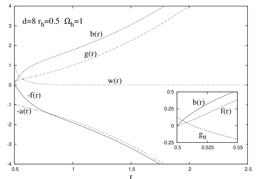
Figure 4: The profiles of the metric functions $a(r)$, $b(r),~{}f(r),~{}g(r)$ and $w(r)$ are shown for a typical $d=8$ rotating black string solution with $r_{h}=0.5$, $\Omega_{H}=1$.

Similarly to the static case, the conserved charged of the black strings are obtained by using the counterterms method in conjunction with the quasilocal formalism. Using the counterterms presented in Section $2$, the computation of $T_{ab}$ is straightforward and we find the following expressions for mass, tension and angular momentum:

$$M=\frac{\ell^{d-4}}{16\pi G_{d}}\big{[}c_{z}-(d-4)c_{t}+(d-4)c_{g}\big{]}L{\cal V}_{d-3}~{},$$ (42)

$${\mathcal{T}}=\frac{\ell^{d-4}}{16\pi G_{d}}\big{[}(d-4)c_{z}-c_{t}-(d-2)c_{g}\big{]}{\cal V}_{{d-3}}~{},~{}~{}~{}J_{(k)}=J=\frac{\ell^{d-4}}{16\pi G_{d}}\frac{(d-1)c_{\varphi}}{d}{\cal V}_{d-3}.$$

A computation similar to that presented in Section $3.3$ leads to the following Smarr-type relation:

$$M+{\mathcal{T}}L-\frac{(d-2)}{2}\Omega_{H}J=T_{H}S,$$ (43)

where as usual the entropy is $S=A_{H}/4G_{d}$.

4.3 Numerical results

The equations (4.1)-(4.1) have been solved for several even values of $d$, special attention being paid to the case $d=6$. This was done since the decay of the relevant parts of the metric functions is lower in the six dimensional case and this leads to better numerical accuracy; also, the properties of the $d=6$ case appear to be generic.

Figure 5: The mass-parameter $M$, the tension ${\mathcal{T}}$, the Hawking temperature $T_{H}$, the entropy $S$ as well as the angular momentum $J$ are represented as functions of the event horizon radius $r_{h}$ for $d=6$ rotating black string solutions with fixed angular momentum $J$ (Figure 5a) and fixed event horizon velocity $\Omega_{H}$ (Figure 5b).

The numerical methods employed here are different from those used to describe the static charged black strings, and we used the differential equation solver $COLSYS$, which involves a Newton-Raphson method [32]. Rotating solutions are found by starting with a static vacuum configuration with a given $r_{h}$ and increasing the value of $\Omega_{H}$ or $J$. The Einstein equations have been solved for a range of $r_{h}$ imposing the appropriate boundary conditions at the horizon and at infinity.

The set of boundary conditions is completely specified by fixing by hand either $\Omega_{H}$ or the angular momentum $J$ through fixing the quantity $c_{\varphi}$. We used both possibilities that, apart from leading to different physical issues for the solution, provide useful consistency cross-checks of the numerical method.

The complete classification of the solutions in the space of parameters is a considerable task that is not aimed in this paper. Instead, by taking $\ell=1$ we analyzed in detail a few particular classes of solutions, which hopefully would reflect all relevant properties of the general pattern. Indeed, as in the charged case discussed in the previous section, the solutions for any other value of the cosmological constant are easily found by using a suitable rescaling of the $\ell=1$ configurations. To this end, and to understand the dependence of the solutions on the cosmological constant, we note that the Einstein equations in the rotating case (4.1)-(35) are left invariant by the following transformation:

$$r\to\bar{r}=\lambda r,~{}~{}\ell\to\bar{\ell}=\lambda\ell,~{}~{}\alpha\to\bar{\alpha}=\lambda^{d-3}\alpha.$$ (44)

Therefore, starting from a solution corresponding to $\ell=1$ one may generate in this way a family of “copies of solutions” with $\ell\neq 1$, with the same length $L$ for the $z-$direction. Their relevant properties, expressed in terms of the corresponding properties of the initial solution, are as follows:

$$\bar{r}_{h}=\lambda r_{h},~{}\bar{\Lambda}=\Lambda/\lambda^{2},~{}\bar{T}_{H}=T_{H}/\lambda,~{}\bar{\Omega}_{H}=\Omega_{H}/\lambda,~{}\bar{M}=\lambda^{d-4}M,~{}\bar{J}=\lambda^{d-3}J,~{}{\rm and}~{}\bar{{\mathcal{T}}}=\lambda^{d-4}{\mathcal{T}}.$$

We first discuss the general features of solutions for a fixed angular velocity of the event horizon. In this case, we were able to construct branches of solutions for increasing $r_{h}$ for several values of $\Omega_{H}$. These branches can alternatively be constructed by keeping $r_{h}$ fixed and increasing the parameter $\Omega_{H}$. In this approach, we observe that the parameter $|w^{\prime}(r_{h})|$ becomes very large (likely infinite) for some maximal value of $\Omega_{H}$. The precise evaluation of this value is not easy because the numerical analysis becomes very involved in this region; for example we obtain solutions up to $\Omega_{H}\leq 1.22$ in the case $r_{h}=0.5$. The maximal value of $\Omega_{H}$ decreases slowly while $r_{h}$ increases.

Again, the metric functions are monotonical functions of $r$, approaching fast the asymptotics (see Figure 4 for a plot of a typical $d=8$ rotating configuration). Examining the component $g_{tt}$ of the metric (see (39)), we can determine the radius, say $r_{e}$, for which $g_{tt}(r_{e})=0$, determining the ergosurface. From the bounday conditions and (39) we can see indeed that $g_{tt}$ takes positive values for a some region $r_{h}<r<r_{e}$, as one can see in the inlet in Figure 4. For a given $r_{h}$, the value of $r_{e}$ increases slightly with $\Omega_{H}$. For example, in the case $d=6$, we find:

$$r_{e}\simeq 0.508\ ,\ 0.525\ ,\ 0.527\ \ {\rm for}\ \ \Omega_{H}=0.5\ ,1.0,\ 1.18\ \ {\rm and}\ \ r_{h}=0.5~{},\ \$$

$$r_{e}\simeq 1.028\ ,\ 1.037\ ,\ 1.042\ \ {\rm for}\ \ \Omega_{H}=0.5\ ,0.7,\ 0.85\ \ {\rm and}\ \ r_{h}=1.0~{}.$$

In the limit $r_{h}\to 0$, the rotating solution becomes singular, for any nonzero value of $\Omega_{H}$. This is indicated by the fact that some of the parameters, namely $b^{\prime}(r_{h}),w^{\prime}(r_{h})$, become infinite in this limit while $J$ tends to zero.

Studying the solutions in the plane $(r_{h},J)$ with $J$ fixed reveals that, for $J>0$, black string solutions exist only for an horizon radius larger than a minimal value, i.e. $r_{h}>r_{h}^{(m)}$ (depending on $J$). This observation is in full agreement with the property discussed above, which states that no regular solution exist for $w\neq 0$. For instance, for $J=0.025$ and $J=0.25$ we find $r_{h}^{(m)}\approx 0.48$ and $r_{h}^{(m)}\approx 0.82$, respectively.

Again, several quantities, namely $b(r_{h}),w(r_{h}),-w^{\prime}(r_{h})$, become very large in the limit $r_{h}\to r_{h}^{(m)}$.

In Figure 5 we present the dependence of various physical parameters on the event horizon radius for $d=6$ solutions with a fixed value of either $J$ or $\Omega_{H}$. These plots retain the basic features of the solutions we found in other dimensions.

5 Thermodynamics of the $k=1$ solutions

As we have mentioned in Section $2$, the thermodynamics of the black objects is usually studied on the Euclidean section. However, for the solutions discussed in this paper it is not possible to find directly real solutions on the Euclidean section by Wick rotating $t\rightarrow i\tau$ the Lorentzian configurations.

Figure 6: Left: The inverse temperature $\beta=1/T_{H}$ ${\it vs.}$ the horizon radius $r_{h}$ for various values of the electric potential $\Phi$. Right: The Gibbs free energy $G$ ${\it vs.}$ the Hawking temperature $T_{H}$ for charged static black strings in the grand-canonical ensemble.

In view of this difficulty one has to resort to an alternative quasi-Euclidean approach. Using this method we computed in Section $3$ the thermodynamic quantities for the electrically charged black string, such as its mass, temperature, entropy, charge and electric potential, while in Section $4$ we considered the similar thermodynamic quantities for the rotating black strings in even dimensions.

Let us consider first the thermodynamics of the charged string. As it is well-known, small Schwarzschild-AdS black holes have negative specific heat (they are unstable) but large size black holes have positive specific heat (and they are stable). It was also found that Schwarzschild-AdS black holes are subjected to the Hawking-Page phase transition [3]: at low temperatures a thermal gas is a globally stable configuration in the AdS background (since in this background, black holes can exist only for temperatures above a critical value) but when one increases the temperature above the critical value, the thermal bath becomes unstable and collapses to form a black hole. The results in [7] indicate that this is the case for $k=1$ AdS vacuum black strings as well. The temperature of these configurations is bounded from below. At low temperatures one has a single bulk solution, corresponding to the thermal globally regular solution.

At higher temperatures, above a critical value, there exist two bulk solutions that correspond to the so-called small (unstable) and large (stable) black string solutions. In [7] it has been suggested that there exists a similar Hawking-Page phase transition for the neutral black string. The entire unstable branch has positive free energy while the free energy of the stable branch goes rapidly negative for temperatures above a critical value. This critical value corresponds then to the temperature at which one observes a phase transition between the large black strings and the thermal globally regular background.

The discussion of the charged case is more involved [5]. One can describe the thermodynamics using two different thermodynamic ensembles. The grand-canonical ensemble is defined by coupling the system to energy and charge reservoirs at fixed temperature $T_{H}$ and fixed electric potential $\Phi$. As we have seen in Section $3$, a computation of the action using quasi-Euclidean methods leads to $I=\beta(M-\Phi Q)-S$, such that the Gibbs free energy is obtained as $G=I/\beta=M-T_{H}S-\Phi Q.$

One can plot the inverse temperature versus the horizon radius as in Figure $6$ (left). Similarly to the RNAdS case one finds that there are two types of behaviour, determined by a critical value, $\Phi_{c}$, of the electric potential $\Phi$. For $\Phi<\Phi_{c}$ one finds that the inverse temperature is bounded and goes smoothly to zero as $r_{h}\rightarrow 0$, while for $\Phi\geq\Phi_{c}$ one finds that $\beta$ diverges when the radius of the extremal black string is reached. A graph of the Gibbs free energy ${\it vs.}$ the Hawking temperature is presented in Figure $6$ for various values of the electric potential $\Phi$ (to simplify the picture, we consider only the $d=5,~{}k=1$ case). In the large potential regime one has only one branch of large black string solutions and one can see that they are stable. In the low potential regime one has two branches of allowed solutions and similarly to the RNAdS case the small black strings are unstable, while the large black strings are stable and dominate the thermodynamics for all temperatures.

Figure 7: Left: The inverse temperature $\beta=1/T_{H}$ ${\it vs.}$ the horizon radius $r_{h}$ for various values of the electric charge $Q$. Right: The free energy $F$ ${\it vs.}$ the Hawking temperature $T_{H}$ for charged static black strings in the canonical ensemble.

If one fixes the value of the charge on the boundary then one deals with the canonical thermodynamic ensemble. The corresponding thermodynamic potential, the Helmholtz potential can be obtained from the Gibbs free energy by means of a Legendre transformation (see also (3)) $F=G+\Phi Q=M-T_{H}S$. A plot in Figure $7$ of the inverse temperature $\beta$ $vs.$ the black string horizon radius $r_{h}$ reveals the very interesting phase structure found previously in the RNAdS case [5]: for small values of the charge, bellow a critical value $Q_{c}$, one finds that one can have three branches of black string solutions, while for large charges, greater than the critical value, one finds only one branch of large black strings, which are thermodynamically stable.

In Figure $7$ we present also a plot of $F$ ${\it vs.}$ temperature for several values of $Q$. The corresponding picture for RNAdS black holes was discussed in [5]. The black string picture here resembles again some of the features of the RNAdS case. Since there are three black string branches for small values of $Q<Q_{c}$ one can see that the free energy presents a part resembling the “swallowtail” shape of [5] as well.

In the small charge regime, for low temperatures, there exists only one branch of black strings (“branch $1$”). However, unlike the RNAdS case this branch is unstable. Increasing the temperature one notices the apparition of two other branches of solutions (“branch $2$” and “branch $3$”) and they separate from each other at higher temperatures. At some temperature the two branches (“branch $1$” and “branch $2$”) coalesce and then disappear, while “branch $3$” carries on till higher temperatures and at high enough temperatures the free energy of “branch $3$” goes rapidly negative and, therefore, this branch dominates the thermodynamics in this regime. If the charge is greater than the critical value, one has only one branch of black strings. At high enough temperatures this branch is thermodynamically stable.

The discussion of the thermodynamic properties of the rotating black string solutions in even dimensions proceeds on similar lines. One has again the choice of two distinct thermodynamic ensembles to describe their physics. The grand-canonical ensemble corresponds in this case to fixing the Hawking temperature $T_{H}$ and the angular velocity $\Omega_{H}$ on the boundary. In this case the thermodynamic Gibbs potential is given by $G=M-T_{H}S-(d-2)\Omega_{H}J/2$.

Figure 8: The entropy is plotted vs. the Hawking temperature for the $k=1$, $d=5$ charged static and the $k=1$, $d=6$ vacuum rotating black string solutions.

There exists again a critical value of $\Omega_{H}$: for values smaller than this critical value one has two branches (one stable and one unstable) of rotating black string solutions, while for values of $\Omega_{H}$ greater than the critical value one obtains only one branch (unstable) of black string solutions. The canonical ensemble corresponds to fixing the Hawking temperature $T_{H}$ and the angular momentum $J$ on the boundary. The thermodynamic potential, which in this case it is Helmholtz’ free energy, can be obtained from the Gibbs potential by means of a Legendre transform $F=G+(d-2)\Omega_{H}J/2=M-T_{H}S$. In this case our results indicate that the situation familiar from the static case remains valid for small values of $J$. For larger $J$, one finds however only one branch of solutions, which becomes stable at high enough temperatures.

One can also attempt a discussion of the local thermodynamic stability of the black string solutions based on the numerical results presented in the previous sections, which are valid for solutions with Lorentzian signature. Our results indicate that the presence of an electric charge or an angular momentum has a tendency to stabilize the black strings. Here we shall restrict to the case of a canonical ensemble, in which case the length of the extra-dimension $L$, the electric charge or the angular momentum are kept fixed. The response function whose sign determines the thermodynamic stability is the heat capacity $C=T\left(\frac{\partial S}{\partial T}\right)_{L,X},$ with $X=Q$ or $J$. As seen in Figure $8$, the picture familiar from the static vacuum case is recovered for small electric charge or a small angular momenta. However, our numerical results suggest that only one branch of stable solutions exist for large enough values of the new global charges. Along this branch the entropy is increasing with the Hawking temperature and, as a result, the solutions have a positive heat capacity and therefore these solutions are locally thermodynamically stable.

6 Einstein-Maxwell-Liouville black holes in lower dimensions

Consider a theory in $d$ dimensions described by the bosonic Lagrangian:

$${\cal L}_{d} = \sqrt{|\tilde{g}|}(\tilde{R}-2\Lambda-\frac{1}{4}\tilde{F}_{(2)}^{2})~{},$$ (45)

where $\tilde{F}_{(2)}=d\tilde{A}_{(1)}$. Assume that the fields are stationary and that the system admits two commuting Killing vectors (one of them is assumed to be timelike). We will perform a dimensional reduction from $d$-dimensions down to $(d-2)$-dimensions along two directions $z$ and $t$. Our metric ansatz is:

$$d\tilde{s}_{d}^{2} = e^{-\sqrt{\frac{2(d-3)}{d-2}}\phi}(dz+{\cal A}_{(1)}^{1}+{\cal A}_{(0)2}^{1}dt)^{2}$$ (46)

$$+e^{\sqrt{\frac{2}{(d-2)(d-3)}}\phi}\bigg{[}-e^{-\sqrt{\frac{2(d-4)}{d-3}}\phi_{1}}(dt+{\cal A}_{(1)}^{2})^{2}+e^{\sqrt{\frac{2}{(d-3)(d-4)}}\phi_{1}}ds_{d-2}^{2}\bigg{]},$$

while the Kaluza-Klein reduction ansatz for the electromagnetic potential field is:

$$\tilde{A}_{(1)}=A_{(1)}+A_{(0)2}dt+A_{(0)1}dz.$$ (47)

In these notations, the bosonic Lagrangean in $(d-2)$ dimensions, obtained by dimensional reduction of the $EM$ theory from $d$-dimensions is given by:

$${\cal L}_{d-2} = \sqrt{|g|}\bigg{[}R-2\Lambda e^{\sqrt{\frac{2}{(d-2)(d-3)}}\phi+\sqrt{\frac{2}{(d-3)(d-4)}}\phi_{1}}-\frac{1}{2}(\partial\phi)^{2}-\frac{1}{2}(\partial\phi_{1})^{2}$$ (48)

$$-\frac{1}{4}e^{-\sqrt{\frac{2}{(d-2)(d-3)}}\phi-\sqrt{\frac{2}{(d-3)(d-4)}}\phi_{1}}(F_{(2)})^{2}+\frac{1}{2}e^{\sqrt{\frac{2(d-4)}{(d-3)}}\phi_{1}-\sqrt{\frac{2(d-2)}{d-3}}\phi}({\cal F}_{(1)2}^{1})^{2}$$

$$-\frac{1}{4}e^{-\sqrt{\frac{2}{(d-3)(d-4)}}\phi_{1}-\sqrt{\frac{2(d-2)}{d-3}}\phi}({\cal F}_{(2)}^{1})^{2}+\frac{1}{4}e^{-\sqrt{\frac{2(d-3)}{d-4}}\phi_{1}}({\cal F}_{(2)}^{2})^{2}$$

$$-\frac{1}{2}e^{\sqrt{\frac{2(d-3)}{(d-2)}}\phi}(F_{(1)1})^{2}+\frac{1}{2}e^{-\sqrt{\frac{2}{(d-2)(d-3)}}\phi+\sqrt{\frac{2(d-4)}{(d-3)}}\phi_{1}}(F_{(1)2})^{2}~{}\bigg{]}.$$

Notice that the kinetic terms of the field strengths that carry an index $2$ (corresponding to the timelike direction $t$) have the opposite signs to the usual ones in a dimensional reduction along a spatial direction. In general, the field strengths that appear in the dimensionally reduced Lagrangian have Chern-Simons type modifications and can be expressed in the following form:

$${\cal F}_{(1)2}^{1} = d{\cal A}_{(0)2}^{1}\equiv d\chi,~{}~{}~{}~{}{\cal F}_{(2)}^{1}={\cal A}_{(1)}^{1}-d\chi\wedge{\cal A}_{(1)}^{2},~{}~{}~{}~{}{\cal F}_{(2)}^{2}=d{\cal A}_{(1)}^{2},~{}~{}~{}~{}F_{(1)1}=dA_{(0)1}$$

$$F_{(1)2} = dA_{(0)2}-\chi dA_{(0)1},~{}~{}~{}~{}F_{(2)}=dA_{(1)}-dA_{(0)1}\wedge({\cal A}_{(1)}^{1}-\chi{\cal A}_{(1)}^{2})-dA_{(0)2}\wedge{\cal A}_{(1)}^{2}~{}.{~{}~{}~{}~{}}$$ (49)

We shall prove now that the above Lagrangian has a global symmetry group $SL(2,R)/O(1,1)$.

First we perform the following field redefinitions:

$${\cal A}_{(1)}^{1} = \hat{{\cal A}}_{(1)}^{1}+\chi\hat{{\cal A}}_{(1)}^{2},~{}~{}~{}{\cal A}_{(1)}^{2}=\hat{{\cal A}}_{(1)}^{2},~{}~{}~{}A_{(1)}=\hat{A}_{(1)}+A_{(0)1}\wedge\hat{{\cal A}}_{(1)}^{1}+A_{(0)2}\wedge\hat{{\cal A}}_{(1)}^{2}$$ (50)

and in terms of the hatted potentials we obtain:

$${\cal F}_{(2)}^{1} = d\hat{{\cal A}}_{(1)}^{1}+\chi d\hat{{\cal A}}_{(1)}^{2},~{}~{}~{}~{}~{}~{}~{}{\cal F}_{(2)}^{2}=d\hat{{\cal A}}_{(1)}^{2},$$ (51)

respectively

$$F_{(2)} = d\hat{A}_{(1)}+A_{(0)1}\wedge d\hat{{\cal A}}_{(1)}^{1}+A_{(0)2}\wedge d\hat{{\cal A}}_{(1)}^{2}$$ (57)

$$= d\hat{A}_{(1)}+\left(\begin{array}[]{cc}A_{(0)2}&A_{(0)1}\end{array}\right)\left(\begin{array}[]{cc}0&1\\ 1&0\end{array}\right)\left(\begin{array}[]{c}\hat{{\cal F}}_{(2)}^{1}\\ \hat{{\cal F}}_{(2)}^{2}\end{array}\right),$$

where $\hat{{\cal F}}_{(2)}^{i}=d\hat{{\cal A}}_{(1)}^{i}$, with $i=1,2$. We make a further rotation of the scalar fields:

$$\left(\begin{array}[]{c}\hat{\phi}\\ \hat{\phi_{1}}\end{array}\right) = \left(\begin{array}[]{cc}\sqrt{\frac{d-4}{2(d-3)}}&\sqrt{\frac{d-2}{2(d-3)}}\\ \sqrt{\frac{d-2}{2(d-3)}}&-\sqrt{\frac{d-4}{2(d-3)}}\end{array}\right)\left(\begin{array}[]{c}\phi\\ \phi_{1}\end{array}\right),$$ (64)

and define the matrix ${\cal M}$ by:

$${\cal M} = \left(\begin{array}[]{cc}e^{-\hat{\phi}_{1}}&\chi e^{-\hat{\phi}_{1}}\\ \chi e^{-\hat{\phi}_{1}}&-e^{\hat{\phi}_{1}}+\chi^{2}e^{-\hat{\phi}_{1}}\end{array}\right).$$ (67)

Note that $\det{\cal M}=-1$ hence ${\cal M}$ is not an $SL(2,R)$ matrix. The $(d-2)$-dimensional Lagrangean can then be written in the following compact form:

$${\cal L}_{d-2} = \sqrt{|g|}(R-2\Lambda e^{\frac{2\hat{\phi}}{\sqrt{(d-2)(d-4)}}}-\frac{1}{2}(\partial\hat{\phi})^{2}+\frac{1}{4}\mbox{tr}[\partial{\cal M}^{-1}\partial{\cal M}]-\frac{1}{4}e^{-\frac{2\hat{\phi}}{\sqrt{(d-2)(d-4)}}}(F_{(2)})^{2}$$ (68)

$$-\frac{1}{4}e^{-\sqrt{\frac{d-2}{d-4}}\hat{\phi}}\hat{{\cal F}}_{(2)}^{T}{\cal M}\hat{{\cal F}}_{(2)}-\frac{1}{2}e^{\sqrt{\frac{d-4}{d-2}}\hat{\phi}}F_{(1)}^{T}({\cal M}^{-1})F_{(1)})~{},$$

where we have defined the column vectors:

$$F_{(1)}=\left(\begin{array}[]{c}dA_{(0)1}\\ dA_{(0)2}\end{array}\right),~{}~{}~{}~{}~{}~{}~{}~{}\hat{{\cal F}}_{(2)}=\left(\begin{array}[]{c}\hat{{\cal F}}_{(2)}^{1}\\ \hat{{\cal F}}_{(2)}^{2}\end{array}\right).$$ (72)

This Lagrangian is manifestly invariant under $SL(2,R)$ transformations if we consider the following transformation laws for the potentials:

$$g_{\mu\nu} \rightarrow g_{\mu\nu},~{}~{}~{}~{}~{}~{}~{}\Lambda\rightarrow\Lambda,~{}~{}~{}~{}~{}~{}~{}{\cal M}\rightarrow~{}\Omega^{T}{\cal M}\Omega,~{}~{}~{}~{}~{}~{}~{}\hat{\phi}\rightarrow\hat{\phi},~{}~{}~{}~{}~{}~{}~{}\hat{A}_{(1)}\rightarrow\hat{A}_{(1)}$$

$$\left(\begin{array}[]{c}\hat{{\cal A}}_{(1)}^{1}\\ \hat{{\cal A}}_{(1)}^{2}\end{array}\right) \rightarrow \Omega^{-1}\left(\begin{array}[]{c}\hat{{\cal A}}_{(1)}^{1}\\ \hat{{\cal A}}_{(1)}^{2}\end{array}\right),~{}~{}~{}~{}~{}\left(\begin{array}[]{c}A_{(0)1}\\ A_{(0)2}\end{array}\right)\rightarrow\Omega^{T}\left(\begin{array}[]{c}A_{(0)1}\\ A_{(0)2}\end{array}\right),$$ (77)

where $\Omega\in SL(2,R)$.

The ansatz (45)-(46) generalizes the transformation considered previously in [7] by the inclusion of an electromagnetic field in the initial Lagrangian in $d$ dimensions and, also, by considering a general stationary metric ansatz in $(d-1)$ dimensions (see also [34] for other work in this direction). Therefore, it is appropriate when treating the charged black string solutions as well as the neutral rotating solutions.

6.1 The electrically charged solutions

Let us apply now this technique to the new solutions presented in this paper. Consider first the case of the electrically charged black strings described in Section $3$. Starting with the $d$ dimensional metric (10) and electromagnetic field (13) and performing a double dimensional reduction along the coordinates $z$ and $t$ we obtain in $(d-2)$ dimensions the following fields:

$$ds_{d-2}^{2} = \left(ab\right)^{\frac{1}{d-4}}\left(\frac{dr^{2}}{f}+r^{2}d\Sigma^{2}_{k,d-3}\right),~{}~{}~{}~{}~{}~{}~{}e^{-\sqrt{\frac{2(d-3)}{d-2}}\phi}=a,~{}~{}~{}~{}~{}~{}~{}e^{-\sqrt{\frac{2(d-4)}{d-3}}\phi_{1}}=ba^{\frac{1}{d-3}},$$

$${\cal A}_{(1)}^{1} = 0,~{}~{}~{}{\cal A}_{(1)2}^{1}\equiv\chi=0,~{}~{}~{}{\cal A}_{(1)}^{2}=0,~{}~{}~{}A_{(1)}=0,~{}~{}~{}A_{(0)2}=2V(r),~{}~{}~{}A_{(0)1}=0.$$ (78)

Let us parameterize the matrix $\Omega$ in the form:

$$\Omega=\left(\begin{array}[]{cc}\alpha&\beta\\ \gamma&\delta\\ \end{array}\right),\qquad\alpha\delta-\beta\gamma=1.$$ (81)

Rotating the scalar fields in $(d-2)$ dimensions and acting with the $SL(2,R)$ transformation $\Omega$ on the corresponding matrix ${\cal M}$, the final scalar fields read:

$$e^{\phi} = (\alpha^{2}a-\gamma^{2}b)^{-\sqrt{\frac{d-2}{2(d-3)}}},~{}~{}~{}~{}~{}~{}~{}e^{\phi_{1}}=(ab)^{-\sqrt{\frac{d-3}{2(d-4)}}}(\alpha^{2}a-\gamma^{2}b)^{-\sqrt{\frac{d-4}{2(d-3)}}},$$ (82)

while the final electromagnetic potentials are given by:

$$A_{(0)1}=2\gamma V(r),~{}~{}~{}~{}~{}~{}~{}A_{(0)2}=2\delta V(r).$$ (83)

Gathering all these results, we obtain in $(d-1)$ dimensions the following fields:

$$ds_{d-1}^{2} = -ab(\alpha^{2}a-\gamma^{2}b)^{-\frac{d-4}{d-3}}dt^{2}+(\alpha^{2}a-\gamma^{2}b)^{\frac{1}{d-3}}\frac{dr^{2}}{f}+r^{2}(\alpha^{2}a-\gamma^{2}b)^{\frac{1}{d-3}}d\Sigma^{2}_{k,d-3},$$ (84)

$$e^{\phi} = (\alpha^{2}a-\gamma^{2}b)^{-\sqrt{\frac{d-2}{2(d-3)}}},~{}~{}~{}~{}~{}{\cal A}_{(1)}=\frac{\alpha\beta a-\gamma\delta b}{\alpha^{2}a-\gamma^{2}b}dt,~{}~{}~{}~{}~{}A_{(0)1}=2\gamma V(r),~{}~{}~{}~{}~{}A_{(0)2}=2\delta V(r).$$

For $F_{(1)1}=dA_{(0)1}$ and $F_{(2)}=dA_{(0)2}\wedge dt$ this gives us a solution of the equations of motion derived from the following Lagrangian:

$${\cal L}_{d-1} = \sqrt{|g|}(R-2\Lambda e^{\sqrt{\frac{2}{(d-2)(d-3)}}\phi}-\frac{1}{2}e(\partial\phi)^{2}-\frac{1}{2}e^{\sqrt{\frac{2(d-3)}{(d-2)}}\phi}(F_{(1)1})^{2}$$ (85)

$$-\frac{1}{4}e^{-\sqrt{\frac{2}{(d-2)(d-3)}}\phi}(F_{(2)})^{2}-\frac{1}{4}e^{-\sqrt{\frac{2(d-2)}{d-3}}\phi}({\cal F}_{(2)})^{2})~{},$$

which corresponds to an Einstein-Dilaton theory with a Liouville potential for the dilaton and coupled with two electromagnetic fields and one scalar field.

6.2 The rotating solutions

Take now the case of the rotating neutral black string solutions in even $d$ dimensions. One can set directly $A_{(1)}=A_{(0)1}=A_{(0)2}=0$ in the initial ansatz for the $d$ dimensional fields and by comparing the metric (33) with the Kaluza-Klein ansatz (46) one reads straightforwardly the following fields in $(d-2)$ dimensions:

$$ds_{d-2}^{2} = \left(a(b-r^{2}w^{2})\right)^{-\frac{1}{2}\sqrt{\frac{d-2}{d-4}}}\bigg{[}\frac{dr^{2}}{f}+g\sum_{i=1}^{N-1}\left(\prod_{j=0}^{i-1}\cos^{2}\theta_{j}\right)d\theta_{i}^{2}+g\sum_{k=1}^{N}\rho_{k}d\varphi_{k}^{2}$$ (87)

$$+\frac{r^{4}(1-w^{2})+r^{2}(b+gw^{2})-bg}{b-r^{2}w^{2}}\left(\sum_{k=1}^{N}\rho_{k}d\varphi_{k}\right)^{2}\bigg{]},$$

$$e^{-\sqrt{\frac{2(d-3)}{d-2}}\phi} = a,~{}~{}e^{-\sqrt{\frac{2(d-4)}{d-3}}\phi_{1}}=(b-r^{2}w^{2})a^{\frac{1}{d-3}},~{}~{}{\cal A}_{(1)}^{2}=\frac{r^{2}\sum_{k=1}^{N}\rho_{k}d\varphi_{k}}{b-r^{2}w^{2}},~{}~{}{\cal A}_{(1)}^{1}=0,~{}~{}{\cal A}_{(0)2}^{1}=0,$$

where we denoted:

$$\rho_{k} = \left(\prod_{l=0}^{k-1}\cos^{2}\theta_{l}\right)\sin^{2}\theta_{k}.$$ (88)

Rotating the scalar fields in $(d-2)$ dimensions and acting with the $SL(2,R)$ transformation $\Omega$ on the corresponding matrix ${\cal M}$, the final scalar fields read:

$$e^{\phi} = \left(\alpha^{2}a-\gamma^{2}(b-r^{2}w^{2})\right)^{-\sqrt{\frac{d-2}{2(d-3)}}},~{}e^{\phi_{1}}=\big{[}a(b-r^{2}w^{2})\big{]}^{-\sqrt{\frac{d-3}{2(d-4)}}}\left(\alpha^{2}a-\gamma^{2}(b-r^{2}w^{2})\right)^{-\sqrt{\frac{d-4}{2(d-3)}}},$$

while the final electromagnetic potentials are given by:

$${\cal A}_{(1)}^{1}=(\alpha\chi-\beta)\frac{r^{2}\sum_{k=1}^{N}\rho_{k}d\varphi_{k}}{b-r^{2}w^{2}},~{}~{}~{}{\cal A}_{(1)}^{2}=\alpha\frac{r^{2}\sum_{k=1}^{N}\rho_{k}d\varphi_{k}}{b-r^{2}w^{2}},$$ (89)

where

$$\chi\equiv{\cal A}_{(0)2}^{1}=\frac{\alpha\beta a-\gamma\delta(b-r^{2}w^{2})}{\alpha^{2}a-\gamma^{2}(b-r^{2}w^{2})}.$$ (90)

Gathering all these results, we obtain in $(d-1)$ dimensions the following fields:

$$ds_{d-1}^{2}=-a(b-r^{2}w^{2})\big{[}\alpha^{2}a-\gamma^{2}(b-r^{2}w^{2})\big{]}^{-\frac{d-4}{d-3}}(dt+{\cal A}_{(1)}^{2})^{2}+\big{[}\alpha^{2}a-\gamma^{2}(b-r^{2}w^{2})\big{]}^{\frac{1}{d-3}}ds_{d-2}^{2},~{}~{}~{}~{}~{}~{}{~{}~{}~{}}$$ (91)

$$e^{\phi}=\left(\alpha^{2}a-\gamma^{2}(b-r^{2}w^{2})\right)^{-\sqrt{\frac{d-2}{2(d-3)}}},~{}{\cal A}_{(1)}=\frac{\alpha\beta a-\gamma\delta(b-r^{2}w^{2})}{\alpha^{2}a-\gamma^{2}(b-r^{2}w^{2})}dt+(\alpha\chi-\beta)\frac{r^{2}\sum_{k=1}^{N}\rho_{k}d\varphi_{k}}{b-r^{2}w^{2}}.~{}~{}{~{}~{}~{}}$$

This gives us a solution of the equations of motion derived from the following Lagrangian:

$${\cal L}_{d-1} = \sqrt{|g|}(R-2\Lambda e^{\sqrt{\frac{2}{(d-2)(d-3)}}\phi}-\frac{1}{2}(\partial\phi)^{2}-\frac{1}{4}e^{-\sqrt{\frac{2(d-2)}{d-3}}\phi}({\cal F}_{(2)})^{2})~{},$$ (92)

which corresponds to an EM-Dilaton theory with a Liouville potential for the dilaton.

As a consistency check of our final solutions, one can see that if one takes $\Omega=I_{2}$ then one obtains the initial charged black string solution (10), respectively the neutral rotating black string solution (33) after oxidizing back to $d$ dimensions. Also, if $\alpha=\delta=\cosh p$ and $\beta=\gamma=\sinh p$ the effect of the $SL(2,R)$ transformation is equivalent to a boost of the initial black string solution in the $z$ direction.

Let us notice that the final solution (6.2) corresponds to a rotating charged black hole solution of the Einstein-Maxwell-Dilaton theory with a Liouville potential for the dilaton, generalizing the static charged black hole solution derived previously in [7], which is recovered from the above by setting $w=0$. For a generic Kaluza-Klein dimensional reduction, if the isometry generated by the Killing vector $\partial/\partial z$ has fixed points then the dilaton $\phi$ will diverge and the $(d-1)$-dimensional metric will be singular at those points. However, this is not the case for our initial black string solutions and therefore the $(d-1)$-dimensional fields are non-singular in the near-horizon limit $r\rightarrow r_{h}$. Indeed, in the near horizon limit $b(r)\rightarrow 0$ while $a(r)\rightarrow a_{0}$ and the $(d-1)$-dimensional fields are non-singular. As with the black hole solution discussed in [7], the situation changes when we look in the asymptotic region. Recall from (46) that

$$g_{zz}\equiv e^{-\sqrt{\frac{2(d-3)}{d-2)}}\phi}=\alpha^{2}a-\gamma^{2}(b-r^{2}w^{2})$$ (93)

gives the radius squared of the $z$-direction in $d$-dimensions and that it diverges in the large $r$ limit. Then for generic values of the parameters in $\Omega$ we find that $g_{zz}\sim r^{2}$ and the dilaton field in $(d-1)$-dimensions will diverge in the asymptotic region. Physically, this means that the spacetime decompactifies at infinity; the higher-dimensional theory should be used when describing such black holes in these regions. On the other hand one can choose the parameters in $\Omega$ such that $\alpha=\gamma$. In this case the asymptotic behaviour of the $(d-1)$-dimensional fields is quite different as $g_{zz}\sim\frac{c_{z}-c_{t}}{r^{d-3}}$ and the radius of the $z$-direction collapses to zero asymptotically. However the dilaton field still diverges at infinity. Also, one can prove that the relevant properties of these solutions can be derived from the corresponding $d-$dimensional seed configurations.

6.3 $T$-dual solutions in $10$ dimensions

Finally, let us make a few remarks about the embedding of our solutions into string/M-theory. Our neutral, rotating black string solutions were being considered in even dimensions only and, therefore, since they admit a negative cosmological constant, one cannot give them a natural interpretation as solutions of string/M-theory. However, the charged $5$-dimensional black string solution can be given such an interpretation. To see this, consider the oxidation back to $d=5$ dimensions of the solution given in (6.1):

$$ds_{5}^{2} = -\frac{ab}{\alpha^{2}a-\gamma^{2}b}dt^{2}+(\alpha^{2}a-\gamma^{2}b)(dz+\frac{\alpha\beta a-\gamma\delta b}{\alpha^{2}a-\gamma^{2}b}dt)^{2}+\frac{dr^{2}}{f}+r^{2}d\Omega^{2},$$ (94)

$$A_{(1)} = \delta V(r)dt+\gamma V(r)dz.$$ (95)

Notice that this solution can be obtained from that of the initial charged black string by making the following coordinate transformation:

$$\left(\begin{array}[]{c}z\\ t\end{array}\right)\rightarrow\Omega\left(\begin{array}[]{c}z\\ t\end{array}\right).$$ (98)

Now, even if the two metrics can be locally isometric by means of the above transformation, their global structure can be completely different since the coordonate transformation considered above mixes the time coordinate $t$ with a periodic spacelike coordinate $z$. This is also apparent from the above discussion in which we have seen that for special values of the parameters in $\Omega$ the asymptotic radius of the $z$-direction differs considerably: in some cases it can grow like $r^{2}$, while in others it can collapse to zero at large distances.

In [5] it was shown how to obtain the $5$-dimensional EM theory with a negative cosmological constant from a Kaluza-Klein reduction of Type IIB supergravity on a $5$-sphere $S^{5}$. The reduction ansatz is given by:

$$ds^{2} = ds_{5}^{2}+\ell^{2}\sum_{i=1}^{3}\bigg{[}d\mu_{i}^{2}+\mu_{i}^{2}\left(d\varphi_{i}+\frac{2}{\sqrt{3}\ell}A_{(1)}\right)^{2}\bigg{]},$$ (99)

where $ds_{5}^{2}$ is the $5$ dimensional metric, $\mu_{i}$ are direction cosines on the $S^{5}$ (with $\sum_{i=1}^{3}\mu_{i}^{2}=1$) and $\varphi_{i}$ are rotation angles on $S^{5}$. The ansatz for the Ramond-Ramond $5$-form was also presented in [5]. One can see that a non-vanishing electromagnetic field $A_{(1)}$ in $5$ dimensions corresponds to a rotation of the $S^{5}$ by equal amounts in each of its three independent rotation planes. Notice now that a point at fixed $\mu_{i}$ and $\varphi_{i}$ on the $S^{5}$ moves on an orbit of $\xi=\partial/\partial t$. For the electric black string solution discussed in Section $3$ the norm of this Killing vector is:

$$\xi^{\mu}\xi_{\mu}=-b(r)+\frac{4}{3}V(r)^{2}.$$ (100)

As explained in [33], the existence of regions where the norm of this vector becomes positive would signal potential instabilities of this metric since in those regions the internal sphere $S^{5}$ would rotate at speeds higher than the velocity of light. Similarly to the RNAdS case discussed in [33], we find that the norm of this Killing vector is always negative and, therefore, the internal sphere $S^{5}$ never rotates at speeds faster than light.

It is also instructive to note that since the black string horizon is translationally invariant along the $z$ direction, one can consider the effect of a $T$-duality along this spacelike direction. We shall focus here on the specific $T$-duality that interchanges the Type IIA with the Type IIB supergravity solutions. The action of $T$-duality on the supergravity fields is easy to write down in the $NS-NS$ sector. However in the $RR$ sector the situation is more complicated as the $RR$ fields transform in the spinorial representation of the $T$-duality group [35, 36]. For a single $T$-duality transformation, say along the spacelike coordinate $z$, in the $NS-NS$ sector we have the following transformation laws [37, 38]:

$$\tilde{G}_{zz} = \frac{1}{G_{zz}},~{}~{}~{}~{}\tilde{G}_{zi}=\frac{B_{zi}}{G_{zz}},~{}~{}~{}~{}\tilde{G}_{ij}=G_{ij}-\frac{G_{zi}G_{zj}-B_{zi}B_{zj}}{G_{zz}},$$

$$\tilde{B}_{zi} = \frac{G_{zi}}{G_{zz}},~{}~{}~{}~{}\tilde{B}_{ij}=B_{ij}-\frac{G_{zi}B_{jz}-G_{zj}B_{iz}}{G_{zz}},~{}~{}~{}~{}e^{2\tilde{\phi}}=\frac{e^{2\phi}}{G_{zz}},$$ (101)

while in the $RR$ sector we have the following transformations laws of the field strengths $F$ [35]:

$$\tilde{F}^{(n)}_{i_{1}\cdots i_{n-1}z} = F^{(n-1)}_{i_{1}\cdots i_{n-1}}-(n-1)G_{zz}^{-1}F^{(n-1)}_{[i_{1}\cdots i_{n-2}z}G_{i_{n}]z},$$

$$\tilde{F}^{(n)}_{i_{1}\cdots i_{n}} = F^{(n+1)}_{i_{1}\cdots i_{n}z}+nF^{(n-1)}_{[i_{1}\cdots i_{n-1}}B_{i_{n}]z}+n(n-1)G_{zz}^{-1}F^{(n-1)}_{[i_{1}\cdots i_{n-2}z}B_{i_{n-1}z}G_{i_{n}]z}~{},$$ (102)

where the indices $i$, $j$ run over all the coordinates except $z$, the anti-symmetrization does not involve the index $z$ and the upper index for the $RR$ field strengths $F^{(n)}$ indicates their rank, with $n=0,2,4,6,8,10$ for Type IIB theory, while $n=1,3,5,7,9$ for Type IIA theory. However, we notice that these field strengths are not independent and they are dual to each other. In consequence the effective action of the respective Type II theory contains only field strengths with $n\leq 4$.

For simplicity, we consider the $10$ dimensional oxidation of the ‘boosted’ neutral black string solution (95). The corresponding ten-dimensional solution of the Type IIB supergravity theory is given by:

$$ds_{10}^{2} = -\frac{ab}{\alpha^{2}a-\gamma^{2}b}dt^{2}+(\alpha^{2}a-\gamma^{2}b)(dz+\frac{\alpha\beta a-\gamma\delta b}{\alpha^{2}a-\gamma^{2}b}dt)^{2}+\frac{dr^{2}}{f}+r^{2}d\Omega^{2}+l^{2}d\Omega_{5}^{2},$$

where $d\Omega_{5}^{2}$ is the metric element of the unit $5$-sphere. This metric is a solution of the Type IIB supergravity equations of motion with the self-dual $5$-from given by [5]:

$$F^{(5)} = -\frac{4}{\ell}\epsilon_{(5)}-\frac{4}{\ell}\star\epsilon_{(5)}.$$ (103)

On components one has:

$$F_{\mu_{1}\mu_{2}\mu_{3}\mu_{4}\mu_{5}} = \frac{4}{\ell}\epsilon_{\mu_{1}\mu_{2}\mu_{3}\mu_{4}\mu_{5}},~{}~{}~{}~{}F_{m_{1}m_{2}m_{3}m_{4}m_{5}}=-\frac{4}{\ell}\epsilon_{m_{1}m_{2}m_{3}m_{4}m_{5}}.$$ (104)

Here the indices $\mu$ are indices on the $AdS_{5}$ sector, while the $m$’s correspond to the indices of the coordinates on the $5$-sphere. Our definition of the Hodge operator $\star$ is such that $\star^{2}F^{(n)}=(-1)^{n+1}F^{(n)}$. Using (101) and (102) one finds:

$$ds_{10}^{2} = -\frac{ab+\left(\alpha\beta a-\gamma\delta b\right)^{2}}{\alpha^{2}a-\gamma^{2}b}dt^{2}+\frac{dz^{2}}{\alpha^{2}a-\gamma^{2}b}+\frac{dr^{2}}{f}+r^{2}d\Omega^{2}+l^{2}d\Omega_{5}^{2},$$

$$B_{zt} = \frac{\alpha\beta a-\gamma\delta b}{\alpha^{2}a-\gamma^{2}b},~{}~{}~{}~{}e^{-2\phi}=\alpha^{2}a-\gamma^{2}b,$$ (105)

$$F^{(4)}_{\mu_{1}\cdots\mu_{4}} = \frac{4}{\ell}\sqrt{\alpha^{2}a-\gamma^{2}b}~{}\epsilon_{\mu_{1}\cdots\mu_{4}},~{}~{}~{}~{}F^{(6)}_{i_{1}\cdots i_{6}}=-\frac{4}{\ell}\sqrt{\alpha^{2}a-\gamma^{2}b}~{}\epsilon_{i_{1}\cdots\i_{6}}$$

where in the above formulae $\mu\neq z$ and $i\neq t,r,\theta,\varphi$, while $\epsilon$ denotes the volume element of the corresponding subspace. It is an easy matter to check that $\star F^{(4)}=F^{(6)}$ while $\star F^{(6)}=-F^{(4)}$ as expected.

Similarly to the case of the $T$-dual geometry of a toroidal black hole described in [39] one finds that the horizon location of the $T$-dual geometry is the same, given by the root $r=r_{h}$ of the equation $f(r)=0$. The asymptotic limit is non-trivial:

$$ds_{10}^{2} \sim \frac{r^{2}}{\ell^{2}}\big{[}-dt^{2}+\ell^{2}d\Omega_{2}^{2}\big{]}+\frac{\ell^{2}}{r^{2}}\big{[}dr^{2}+dz^{2}]+\ell^{2}d\Omega_{5}^{2},$$ (106)

for generic values of the parameters describing the $SL(2,R)$ transformation $\Omega$. Apart from the metric element of the $5$-sphere $S^{5}$ one notices that the topology at large $r$ is a warped product of a $3$-dimensional Einstein universe with a $2$-dimensional hyperbolic space (compactified along the $z$ direction). However, for the special values of the parameters in $\Omega$, such that $\alpha=\gamma$, one finds that asymptotically the radius of the $z$ direction grows like $r^{2}$ and therefore the topology of the $5$-dimensional part of the metric is very similar to the topology of the initial black string solution.

7 Summary and Discussion

In this paper we have presented arguments for the existence of static electrically charged as well as neutral rotating black string-type solutions of Einstein gravity with negative cosmological constant. These are the AdS natural counterparts of the $\Lambda=0$ uniform black string solutions. The first configuration, discussed in Section $3$, generalized the neutral black string configurations of Ref. [6, 7] by coupling them to an electromagnetic field. In Section $4$ we described a rotating generalization of the black strings in even dimensions only, with equal angular momenta. Different from the neutral case, no vortex-type solution was found in these cases. A discussion of the thermodynamical features of the black string solutions was presented in Section $5$. It is interesting to note that in all considered cases (inclusing the static neutral solutions in [7]), the thermodynamics of the black strings appears to follow the pattern of the corresponding black hole solutions with spherical horizons in AdS backgrounds.

On general grounds, one expects the black objects with a boundary topology $R\times S^{d-3}\times S^{1}$ to present a richer phase structure than in the usual $R\times S^{d-3}$ case (with $R$ corresponding to the time direction), as the radius of the circle introduces another macroscopic scale in the theory. For example, it is well-known that $\Lambda=0$ uniform black strings are affected by the Gregory-Laflamme (GL) instability [40]. That is, for a given circle size, the black objects with translational symmetry bellow a critical mass are linearly unstable. At the critical mass, the marginal mode is static, indicating a new branch of solutions with spontaneously broken translational invariance along the compact direction.

Gregory and Laflamme also noted that the entropy of a fully $d$-dimensional black hole is greater than that of the black string with same mass, when $L$ is large enough. This argument applies also to some of the $\Lambda<0$ vacuum black string solutions, which are likely to present a GL instability. This issue is currently under study as well as the issue of AdS nonuniform black strings, with a dependence on the $z-$coordinate.

However, charges could prevent the instability of the black object since they could contribute some repulsive forces as the horizon shrinks. Gubser and Mitra [41] have proposed an interesting conjecture about the relationship between the classical black string/brane instability and the local thermodynamic stability. This conjecture asserts that the GL instability of the black objects occur iff they are (locally) thermodynamically unstable. The solutions discussed in this paper provide a new laboratory to test this conjecture. Some of them are likely to be stable to linear perturbations.

Another class of $\Lambda<0$ solutions expected to exist for the same structure of the conformal infinity are black holes that do not wrap the circle direction. These solutions would present an $S^{d-2}$ event horizon topology, their approximate form in the near horizon zone being

$$ds^{2}=\frac{d\rho^{2}}{1-\rho_{0}^{d-3}/\rho^{d-3}}+\rho^{2}(d\chi^{2}+\sin^{2}\chi d\Omega_{d-3}^{2})-(1-\rho_{0}^{d-3}/\rho^{d-3})dt^{2}+f_{ij}dx^{i}dx^{j}~{},$$

(where $r=\rho\sin\chi$, $z=\rho\cos\chi$ while $f_{ij}$ are small corrections), the zeroth order corresponding to the $d-$dimensional Schwarzschild metric. Their leading order asymptotic expansion will be similar to that of the black string solutions as given in (15), (18). These would represent the AdS counterparts of the $\Lambda=0$ black hole solutions in Kaluza-Klein theory discussed $e.g.$ in [42].

We expect the solutions considered in this paper to be relevant in the context of AdS/CFT and more generally in the context of gauge/gravity dualities. Indeed, as it has been argued at length in [5], physical properties of the RNAdS black holes in $d$ dimensions can be related by means of the AdS/CFT correspondence to the physics of a class of $(d-1)$-dimensional field theories that are coupled to a global background $U(1)$ current. The $k=1$ solutions presented in this paper describe $\Lambda<0$ electrically charged and also rotating black strings that have horizons with topology $S^{1}\times S^{d-3}$ and conformal boundary $R\times S^{1}\times S^{d-3}$. According to the AdS/CFT correspondence, their properties should be similarly related to those of a dual field theory living on the AdS boundary. In particular, the background metric upon which the dual field theory resides is found by taking the rescaling $h_{ab}=\lim_{r\rightarrow\infty}\frac{\ell^{2}}{r^{2}}\gamma_{ab}$. For $k=1$ black strings we find that for both charged static and neutral rotating solutions the rescaled boundary metric is:

$$ds^{2}=h_{ab}dx^{a}dx^{b}=-dt^{2}+dz^{2}+\ell^{2}d\Omega_{d-3}^{2},$$ (107)

so that the conformal boundary is indeed $R\times S^{1}\times S^{d-3}$.

The expectation value of the stress tensor of the dual field theory can be computed using the relation [43]:

$$\sqrt{-h}h^{ab}<\tau_{bc}>=\lim_{r\rightarrow\infty}\sqrt{-\gamma}\gamma^{ab}T_{bc}.$$ (108)

Restricting for instance to the case of the electrically charged black strings in $5$ dimensions, one can see directly that in the asymptotic expansion (15) or (18) of the metric functions there is no effect of the electric charge in the leading order terms and, therefore, when computing the boundary stress-energy tensor one obtains the same components as those corresponding to an uncharged black string [7]. It is then apparent that the stress-tensor is finite and covariantly conserved, while its trace matches precisely the conformal anomaly of the boundary CFT.

Let us consider now the $d=6$ rotating black string solutions described in Section $4$. For these solutions we find the following non-vanishing components of the boundary stress-energy tensor:

$$~{}<\tau^{z}_{z}>=-\frac{2c_{g}+c_{t}-4c_{z}}{16\pi G_{6}\ell},~{}<\tau^{\theta}_{\theta}>=\frac{3c_{g}-c_{t}-c_{z}}{16\pi G_{6}\ell},~{}~{}<\tau^{\varphi_{1}}_{\varphi_{1}}>=\frac{c_{g}(1+5\cos 2\theta)-2(c_{t}+c_{z})}{32\pi G_{6}\ell}~{},~{}~{}{~{}~{}}$$

$$<\tau_{\varphi_{2}}^{\varphi_{2}}>=\frac{c_{g}(1-5\cos 2\theta)-2(c_{t}+c_{z})}{32\pi G_{6}\ell},~{}<\tau_{\varphi_{1}}^{t}>=\frac{c_{\varphi}\ell\sin^{2}\theta}{16\pi G_{6}},~{}<\tau^{\varphi_{1}}_{t}>=<\tau^{\varphi_{2}}_{t}>=-\frac{5c_{g}}{16\pi G_{6}\ell},~{}$$

$$<\tau_{\varphi_{2}}^{t}>=\frac{c_{\varphi}\ell\cos^{2}\theta}{16\pi G_{6}},~{}<\tau^{\varphi_{2}}_{\varphi_{1}}>=-\frac{5c_{g}\sin^{2}\theta}{16\pi G_{6}\ell},~{}<\tau^{\varphi_{1}}_{\varphi_{2}}>=-\frac{5c_{g}\cos^{2}\theta}{16\pi G_{6}\ell},~{}<\tau^{t}_{t}>=\frac{4c_{t}-c_{z}-2c_{g}}{16\pi G_{6}\ell}.$$

This stress-tensor is traceless, as expected from the absence of conformal anomalies for the boundary field theory in odd dimensions.

More interesting is the situation for the electric black string in seven dimensions. First, notice that the boundary stress-tensor components are the same with those corresponding to the neutral black string. Therefore, we shall discuss first the case of the uncharged black string in seven dimensions. Indeed, a direct computation of the boundary stress-tensor leads to the following components:

$$<\tau^{t}_{t}>=\frac{4000c_{t}-800c_{z}+63}{12800\pi G_{7}\ell},~{}<\tau^{z}_{z}>=\frac{4000c_{z}-800c_{t}+63}{12800\pi G_{7}\ell},~{}<\tau^{\theta}_{\theta}>=-\frac{1600c_{t}+1600c_{z}+117}{25600\pi G_{7}\ell},$$

where by $\theta$ we denote the four angular coordinates on the unit sphere $S^{4}$.

This boundary stress-tensor is finite and covariantly conserved. One can also compute its trace and one obtains simply:

$$<\tau^{a}_{a}>=-\frac{27}{3200\pi G_{7}\ell}.$$ (109)

As expected from the counterterm Lagrangian, it can be checked directly that this trace equals the conformal anomaly [23]:

$${\cal A}=-\frac{\ell^{5}}{128}\left(\mathsf{RR}^{ab}\mathsf{R}_{ab}-\frac{3}{25}\mathsf{R}^{3}-2\mathsf{R}^{ab}\mathsf{R}^{cd}\mathsf{R}_{acbd}-\frac{1}{10}\mathsf{R}^{ab}\nabla_{a}\nabla_{b}\mathsf{R}+\mathsf{R}^{ab}\Box\mathsf{R}_{ab}-\frac{1}{10}\mathsf{R}\Box\mathsf{R}\right).$$ (110)

According to the AdS/CFT conjecture, this trace anomaly in $6$ dimensions should correspond to the trace anomaly of a class of $6$-dimensional non-trivial CFT with maximal supersymmetry, namely the ${\cal N}=(0,2)$ interacting superconformal theories describing $N$ coincident M5 branes [23].

In general, according to the classification given in [44] one can divide the trace anomalies into Type A, which are proportional with the topological Euler density, Type B, which are made-up out of Weyl invariants computed using the Weyl tensor, and also, trivial anomalies, which can be expressed as total derivatives and can be cancelled by the variation of a finite covariant counterterm added to the action. Therefore, the trace anomaly can be expressed in $6$ dimensions as [23]:

$${\cal A}=-\frac{2a_{(6)}}{16\pi G_{7}}=-\frac{6\ell^{5}}{8\pi G_{7}}\left(E_{(6)}+I_{(6)}+\nabla_{i}J^{i}\right),$$ (111)

where $E_{(6)}$ is a term proportional to the Euler density $E_{6}$ in $6$ dimensions, $I_{(6)}$ is a Weyl invariant term constructed using the $3$ Weyl invariants in $6$ dimensions, while $\nabla_{i}J^{i}$ is a trivial anomaly. Before we write the trace anomaly in this form, we shall express it in terms of field theory quantities by using the relation $\ell^{5}/G_{7}=16N^{3}/3\pi^{2}$ [23].

Using now the expressions defined in Appendix, we have [45]:

$${\cal A}=-\frac{4N^{3}}{\pi^{3}}\bigg{[}\frac{1}{2^{11}3^{2}}\left(E_{6}+8(12I_{1}+3I_{2}-I_{3})+\frac{2}{35}\nabla_{i}J^{i}\right)\bigg{]},$$ (112)

where

$$\nabla_{i}J^{i} = 420C_{3}-504C_{4}-840C_{5}-84C_{6}+1680C_{7}.$$ (113)

When evaluated on the boundary geometry corresponding to the black string solution, we obtain $E_{6}=0$, $\nabla_{i}J^{i}=0$, while $I_{1}=-51/100\ell^{6}$, $I_{2}=39/25\ell^{6}$ and $I_{3}=-684/25\ell^{6}$. One can now check explicitly that the above expression gives precisely the anomaly (110).

It is of interest to compare the above result with that corresponding to another maximally supersymmetric CFT in $6$ dimensions: namely the non-interacting one, made up by $N$ copies of the free ${\cal N}=(0,2)$ tensor multiplet containing five scalars, one two-form with selfdual field strength and two Weyl fermions [45, 46]. The conformal anomaly for the free $(2,0)$ tensor multiplet was computed in [45]:

$${\cal A}^{free}=-\frac{1}{\pi^{3}}\bigg{[}\frac{1}{2^{11}3^{2}}\left(\frac{7}{4}E_{6}+8(12I_{1}+3I_{2}-I_{3})+\frac{2}{35}\nabla_{i}{\cal J}^{i}\right)\bigg{]},$$ (114)

where

$$\nabla_{i}{\cal J}^{i}=56C_{2}-420C3-420C_{5}-210C_{6}+840C_{7}.$$ (115)

Apart from the expected factor of $4N^{3}$ [45], one notices that in the black string background the two anomalies are basically the same (since for this background the Euler density is identically zero, while $\nabla_{i}{\cal J}^{i}=0$ as well).

As we have previously mentioned, at leading order the components of the boundary stress-energy tensor do not exhibit any explicit dependence on the electric charge and therefore much of the above discussion regarding the conformal anomaly carries through. Since the $7$-dimensional gauged supergravities that appear from compactifications of $11$-dimensional supergravity do not admit a truncation to pure EM theories with negative cosmological constant, it is then apparent that the electric black string solution cannot be embedded into any such $7$-dimensional gauged supergravity. For this reason the nature of the dual boundary field theory is unknown. However, in the spirit of AdS/CFT correspondence, the charge carried by these solutions can be accounted for by switching on a background global $U(1)$ current (or its canonical conjugate charge) to which the dual field theory couples.

As avenues for further research, it might be interesting to study the more general case of charged and rotating AdS black string solutions, to which the solutions discussed in this paper would be particular cases. However, a more complicated action principle than (1) is required in order to provide a consistent embedding in higher dimensional gauged supergravities (in $10$ and $11$ dimensions) of these solutions. For example, in $d=5$, the simplest supergravity model contains a Chern-Simons term. For the static black string solution discussed in this paper it is obvious that this term is trivially zero. However, it cannot be neglected when discussing general charged rotating black string solutions.

Acknowledgements
The work of ER was carried out in the framework of Enterprise–Ireland Basic Science Research Project SC/2003/390 of Enterprise-Ireland. YB is grateful to the Belgian FNRS for financial support.

Appendix

Following the discussion in [46, 45] we use the following basis of $17$ curvature invariants:

$$\begin{array}[]{lll}K_{1}=R^{3}~{},&K_{2}=RR_{ab}^{2}~{},&K_{3}=RR_{abmn}^{2}~{},\\ &&\\ K_{4}=R_{a}{}^{m}R_{m}{}^{i}R_{i}{}^{a}~{},&K_{5}=R_{ab}R_{mn}R^{mabn}~{},&K_{6}=R_{ab}R^{amnl}R^{b}{}_{mnl}~{},\\ &&\\ K_{7}=R_{ab}{}^{mn}R_{mn}{}^{ij}R_{ij}{}^{ab}~{},&K_{8}=R_{amnb}R^{mijn}R_{i}{}^{ab}{}_{j}~{},&K_{9}=R\nabla^{2}R~{},\\ &&\\ K_{10}=R_{ab}\nabla^{2}R^{ab}~{},&K_{11}=R_{abmn}\nabla^{2}R^{abmn}~{},&K_{12}=R^{ab}\nabla_{a}\nabla_{b}R~{},\\ &&\\ K_{13}=(\nabla_{a}R_{mn})^{2}~{},&K_{14}=\nabla_{a}R_{bm}\nabla^{b}R^{am}~{},&K_{15}=(\nabla_{i}R_{abmn})^{2}~{},\\ &&\\ K_{16}=\nabla^{2}R^{2}~{},&K_{17}=\nabla^{4}R~{}.&\end{array}$$ (A-12)

Then a basis for the non-trivial anomalies in six dimensions can be written as:

$$M_{1} = \frac{19}{800}K_{1}-\frac{57}{160}K_{2}+\frac{3}{40}K_{3}+\frac{7}{16}K_{4}-\frac{9}{8}K_{5}-\frac{3}{4}K_{6}+K_{8},$$

$$M_{2} = \frac{9}{200}K_{1}-\frac{27}{40}K_{2}+\frac{3}{10}K_{3}+\frac{5}{4}K_{4}-\frac{3}{2}K_{5}-3K_{6}+K_{7},$$

$$M_{3} = -K_{1}+8K_{2}+2K_{3}-10K_{4}+10K_{5}-\frac{1}{2}K_{9}+5K_{10}-5K_{11},$$

$$M_{4} = -K_{1}+12K_{2}-3K_{3}-16K_{4}+24K_{5}+24K_{6}-4K_{7}-8K_{8},$$

$$M_{5} = 6K_{6}-3K_{7}+12K_{8}+K_{10}-7K_{11}-11K_{13}+12K_{14}-4K_{15},$$

$$M_{6} = -\frac{1}{5}K_{9}+K_{10}+\frac{2}{5}K_{12}+K_{13},$$ (A-13)

$$M_{7} = K_{4}+K_{5}-\frac{3}{20}K_{9}+\frac{4}{5}K_{12}+K_{14},$$

$$M_{8} = -\frac{1}{5}K_{9}+K_{11}+\frac{2}{5}K_{12}+K_{15},$$

$$M_{9} = K_{16},~{}~{}~{}M_{10}=K_{17}~{}.$$

From these quantities one can form the following trivial anomalies:

$$C_{1}=M_{10},\ \ \ C_{2}=\frac{1}{2}M_{9},\ \ \ C_{3}=-\frac{1}{12}M_{9}+(K_{10}+K_{13}),$$

$$C_{4}=-\frac{7}{6}M_{6}+M_{7}-\frac{5}{72}M_{9}+\frac{7}{6}(K_{10}+K_{13}),\ \ \ C_{5}=-M_{6}+M_{8}+\frac{1}{20}M_{9},$$ (A-14)

$$C_{6}=2M_{6}-M_{7}+\frac{1}{8}M_{9}-2(K_{10}+K_{13}),\ \ C_{7}=\frac{1}{12}M_{5}-\frac{1}{12}M_{6}-\frac{1}{4}M_{7}+\frac{7}{12}M_{8}+\frac{1}{32}M_{9}.$$

Finally, one is now ready to compute the topological Euler density in $6$ dimensions and the three Weyl invariants [46]:

$$E_{6} = 8M_{4}~{},~{}~{}~{}~{}~{}I_{1}=M_{1}~{},~{}~{}~{}~{}~{}I_{2}=M_{2}~{},$$

$$I_{3} = \frac{16}{3}M_{1}+\frac{8}{3}M_{2}-\frac{1}{5}M_{3}+\frac{2}{3}M_{4}-\frac{2}{3}M_{5}-\frac{13}{3}M_{6}+2M_{7}+\frac{1}{3}M_{8}~{}.$$ (A-15)

References

• [1] J. M. Maldacena, Adv. Theor. Math. Phys.  2 (1998) 231 [Int. J. Theor. Phys.  38 (1999) 1113] [arXiv:hep-th/9711200].
• [2] E. Witten, Adv. Theor. Math. Phys.  2 (1998) 253 [arXiv:hep-th/9802150].
• [3] S. W. Hawking and D. N. Page, Commun. Math. Phys.  87 (1983) 577.
• [4] E. Witten, Adv. Theor. Math. Phys.  2 (1998) 505 [arXiv:hep-th/9803131].
• [5] A. Chamblin, R. Emparan, C. V. Johnson and R. C. Myers, Phys. Rev. D 60 (1999) 064018 [arXiv:hep-th/9902170]; A. Chamblin, R. Emparan, C. V. Johnson and R. C. Myers, Phys. Rev. D 60 (1999) 104026 [arXiv:hep-th/9904197].
• [6] K. Copsey and G. T. Horowitz, JHEP 0606 (2006) 021 [arXiv:hep-th/0602003].
• [7] R. B. Mann, E. Radu and C. Stelea, JHEP 0609 (2006) 073 [arXiv:hep-th/0604205].
• [8] G. T. Horowitz and A. Strominger, Nucl. Phys. B 360 (1991), 197.
• [9] A. Chamblin, S. W. Hawking and H. S. Reall, Phys. Rev.  D 61 (2000) 065007 [arXiv:hep-th/9909205].
• [10] A. H. Chamseddine and W. A. Sabra, Phys. Lett. B 477, 329 (2000) [arXiv:hep-th/9911195]. D. Klemm and W. A. Sabra, Phys. Rev. D 62, 024003 (2000) [arXiv:hep-th/0001131]. W. A. Sabra, Phys. Lett. B 545, 175 (2002) [arXiv:hep-th/0207128].
• [11] R. Mann and C. Stelea, Class. Quant. Grav.  21, 2937 (2004) [arXiv:hep-th/0312285].
• [12] H. Lu, D. N. Page and C. N. Pope, Phys. Lett. B 593, 218 (2004) [arXiv:hep-th/0403079]; R. B. Mann and C. Stelea, Phys. Lett. B 634, 448 (2006) [arXiv:hep-th/0508203].
• [13] D. Astefanesei, R. B. Mann and E. Radu, JHEP 0501 (2005) 049 [arXiv:hep-th/0407110]; D. Astefanesei, R. B. Mann and E. Radu, Phys. Lett.  B 620 (2005) 1 [arXiv:hep-th/0406050].
• [14] D. Astefanesei and G. C. Jones, JHEP 0506, 037 (2005) [arXiv:hep-th/0502162]; D. Astefanesei, R. B. Mann and C. Stelea, JHEP 0601, 043 (2006) [arXiv:hep-th/0508162].
• [15] R. B. Mann and C. Stelea, Phys. Lett. B 632, 537 (2006) [arXiv:hep-th/0508186]; A. M. Awad, Class. Quant. Grav.  23, 2849 (2006) [arXiv:hep-th/0508235]; M. H. Dehghani and A. Khodam-Mohammadi, Phys. Rev. D 73, 124039 (2006) [arXiv:hep-th/0604171].
• [16] R. C. Myers and M. J. Perry, Annals Phys.  172 (1986) 304.
• [17] S. W. Hawking, C. J. Hunter and M. M. Taylor-Robinson, Phys. Rev. D 59 (1999) 064005 [arXiv:hep-th/9811056].
• [18] G. W. Gibbons, H. Lu, D. N. Page and C. N. Pope, Phys. Rev. Lett.  93, 171102 (2004) [arXiv:hep-th/0409155]. G. W. Gibbons, H. Lu, D. N. Page and C. N. Pope, J. Geom. Phys.  53, 49 (2005) [arXiv:hep-th/0404008].
• [19] J. Kunz, F. Navarro-Lerida and J. Viebahn, Phys. Lett. B 639 (2006) 362 [arXiv:hep-th/0605075].
• [20] S. W. Hawking and S. F. Ross, Phys. Rev. D 52, 5865 (1995) [arXiv:hep-th/9504019].
• [21] V. Balasubramanian and P. Kraus, Commun. Math. Phys. 208 (1999) 413 [arXiv:hep-th/9902121].
• [22] S. Das and R. B. Mann, JHEP 0008 (2000) 033 [arXiv:hep-th/0008028].
• [23] K. Skenderis, Int. J. Mod. Phys. A 16 (2001) 740, [arXiv:hep-th/0010138]; M. Henningson and K. Skenderis, JHEP 9807 (1998) 023 [arXiv:hep-th/9806087]; M. Henningson and K. Skenderis, Fortsch. Phys.  48, 125 (2000) [arXiv:hep-th/9812032].
• [24] M. Cvetic and S. S. Gubser, J. High Energy Phys. 04, 024 (1999); M. M. Caldarelli, G. Cognola and D. Klemm, Class. Quant. Grav. 17, 399 (2000).
• [25] G. W. Gibbons and S. W. Hawking, Phys. Rev.  D 15 (1977) 2752.
• [26] S. W. Hawking in General Relativity. An Einstein Centenary Survey, edited by S. W. Hawking and W. Israel, (Cambridge, Cambridge University Press, 1979).
• [27] J. D. Brown, E. A. Martinez and J. W. York, Phys. Rev. Lett. 66 2281 (1991); J. D. Brown and J.W. York, Phys. Rev. D47 1407 (1993); Phys. Rev. D47 1420 (1993), [arXiv:gr-qc/9405024]; I. S. Booth and R. B. Mann, Phys. Rev. Lett.  81, 5052 (1998) [arXiv:gr-qc/9806015]; I. S. Booth and R. B. Mann, Nucl. Phys.  B 539, 267 (1999) [arXiv:gr-qc/9806056].
• [28] D. Astefanesei and E. Radu, Phys. Rev.  D 73 (2006) 044014 [arXiv:hep-th/0509144]; H. Elvang, R. Emparan and A. Virmani, JHEP 0612 (2006) 074 [arXiv:hep-th/0608076].
• [29] R. Clarkson, A. M. Ghezelbash and R. B. Mann, Nucl. Phys.  B 674, 329 (2003) [arXiv:hep-th/0307059]; R. B. Mann and C. Stelea, Phys. Rev.  D 72, 084032 (2005) [arXiv:hep-th/0408234].
• [30] T. Harmark and N. A. Obers, Nucl. Phys. B 684 (2004) 183 [arXiv:hep-th/0309230].
• [31] J. Kunz, F. Navarro-Lerida and E. Radu, [arXiv:gr-qc/0702086].
• [32] U. Ascher, J. Christiansen, R. D. Russell, Math. of Comp. 33 (1979) 659; U. Ascher, J. Christiansen, R. D. Russell, ACM Trans. 7 (1981) 209.
• [33] S. W. Hawking and H. S. Reall, Phys. Rev.  D 61, 024014 (2000) [arXiv:hep-th/9908109].
• [34] C. Charmousis, D. Langlois, D. Steer and R. Zegers, JHEP 0702 (2007) 064 [arXiv:gr-qc/0610091].
• [35] S. F. Hassan, Nucl. Phys.  B 568, 145 (2000) [arXiv:hep-th/9907152].
• [36] S. F. Hassan, Nucl. Phys.  B 583, 431 (2000) [arXiv:hep-th/9912236].
• [37] T. H. Buscher, Phys. Lett.  B 201 (1988) 466;
T. H. Buscher, Phys. Lett.  B 194 (1987) 59.
• [38] E. Bergshoeff, C. M. Hull and T. Ortin, Nucl. Phys.  B 451, 547 (1995) [arXiv:hep-th/9504081].
• [39] M. Rinaldi, Phys. Lett.  B 547, 95 (2002) [arXiv:hep-th/0208026].
• [40] R. Gregory and R. Laflamme, Phys. Rev. Lett.  70 (1993) 2837 [arXiv:hep-th/9301052].
• [41] S. S. Gubser and I. Mitra, JHEP 0108, 018 (2001) [arXiv:hep-th/0011127].
• [42] H. Kudoh and T. Wiseman, Phys. Rev. Lett.  94 (2005) 161102 [arXiv:hep-th/0409111].
• [43] R. C. Myers, Phys. Rev. D 60, 046002 (1999) [arXiv:hep-th/9903203].
• [44] S. Deser and A. Schwimmer, Phys. Lett.  B 309, 279 (1993) [arXiv:hep-th/9302047].
• [45] F. Bastianelli, S. Frolov and A. A. Tseytlin, JHEP 0002, 013 (2000) [arXiv:hep-th/0001041].
• [46] F. Bastianelli, G. Cuoghi and L. Nocetti, Class. Quant. Grav.  18, 793 (2001) [arXiv:hep-th/0007222].