Predicting the Cosmological Constant from the Causal Entropic Principle

Abstract:

We compute the expected value of the cosmological constant in our universe from the Causal Entropic Principle. Since observers must obey the laws of thermodynamics and causality, the principle asserts that physical parameters are most likely to be found in the range of values for which the total entropy production within a causally connected region is maximized. Despite the absence of more explicit anthropic criteria, the resulting probability distribution turns out to be in excellent agreement with observation. In particular, we find that dust heated by stars dominates the entropy production, demonstrating the remarkable power of this thermodynamic selection criterion. The alternative approach—weighting by the number of “observers per baryon”—is less well-defined, requires problematic assumptions about the nature of observers, and yet prefers values larger than present experimental bounds.

1 Introduction

The discovery that the universe is in a period of accelerated expansion [1, 2], combined with an accurate accounting of the total, matter, and radiation components of the energy density [3], provide overwhelming evidence for dark energy. These measurements are completely consistent with the interpretation of dark energy as a non-zero cosmological constant, $\Lambda$. This has undermined the hope that the energy of our vacuum is uniquely determined by fundamental theory. Instead, it lends credence to the hypothesis that the cosmological constant is an environmental variable, which takes on different values in widely separated regions of the universe.

The observed vacuum energy density

$$\rho_{\Lambda}=\frac{\Lambda}{8\pi}=(1.25\pm 0.25)\times 10^{-123}~{},$$ (1)

is at least $55$ orders of magnitude smaller than what would be expected from the standard model of particle physics (see, e.g., Ref. [5] for a recent review). The environmental approach does not assert that this tiny value is inevitable, or even typical among all possible values. Rather, it aims to show that it is not atypical among values measured by observers.

A number of conditions must be satisfied for the environmental approach to work. The first, obviously, is that fundamental theory must admit the observed value of the vacuum energy. This can happen without explicit tuning if the theory gives rise to an enormous number $N$ of different vacua. Of course, typical values will be of order unity, but if they are randomly distributed, they can form a dense spectrum, or “discretuum”, with average spacing of order $1/N$. If $N\gg 10^{123}$, then it is likely that the observed value is included in the spectrum. Thus, the approach really depends on whether fundamental theory (which, presumably, is more or less unique) admits a sufficiently dense discretuum.

The second condition is that the observed value must be dynamically attainable, starting from generic initial conditions. With $N\gg 10^{123}$ possibilities, there is no reason for the universe to start out in a vacuum like ours. The environmental approach therefore depends on a means to start from some generic initial value and later realize the observed value, either as a branch in the wavefunction or as a particular spacetime region embedded in a vast universe.

Finally, the environmental approach requires an explanation of why we happen to observe such an unusually small vacuum energy. Most values of $\rho_{\Lambda}$ in the discretuum will be of order unity, and only a fraction (in the simplest case, a fraction of order $10^{-123}$) will have a magnitude as small as the observed value. It is not enough to show that the small value given by Eq. (1) is possible; one must also show that it is not unlikely to be observed.

The first condition appears to be satisfied by string theory, which admits as many as $10^{500}$ long-lived metastable vacua [6, 7, 8, 9, 10] (see Ref. [11] for a discussion of earlier work). The second condition can then be met because the vacua are metastable and can decay into one another.

In this paper we address the third condition. We will use a novel approach, the Causal Entropic Principle, to argue that the observed value of $\rho_{\Lambda}$ is not unlikely. Our main result is shown in Fig. 1.

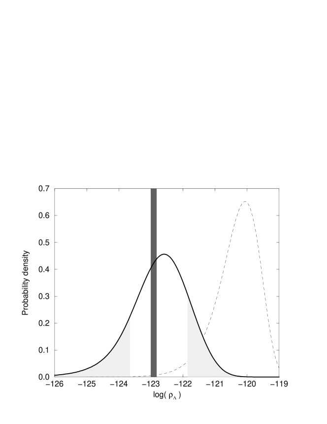
Figure 1: The probability distribution of the vacuum energy measured by typical observers, computed from the Causal Entropic Principle, is shown as a solid curve. The values consistent with present cosmological data, in the shaded vertical bar, are well inside the $1\sigma$ region (shown in white), and hence, not atypical. For comparison, the dashed line shows the distribution derived by estimating the number of observers per baryon. Unlike our curve, it assumes that galaxies are necessary for observers; yet, the observed value is very unlikely under this distribution. For more details about both curves, see Figures 2 and 8.

The Causal Entropic Principle is based on two ideas: any act of observation increases the entropy, and spacetime regions that are causally inaccessible should be disregarded. It assumes that on average, the number of observations will be proportional to the amount of matter entropy produced in a causally connected region, $\Delta S$. Vacua should be weighted by this factor to account for the rate at which they will be observed.

Crucially, the size of the causal diamond is inversely proportional to the vacuum energy, so smaller values of $\rho_{\Lambda}$ allow for greater complexity. This compensates for the scarcity of vacua with small $\rho_{\Lambda}$. As a result, $\rho_{\Lambda}$ prefers to take a value such that vacuum energy begins to dominate near the time of peak entropy production.

We will find that entropy production in the causal diamond is dominated by dust particles heated by stars. This is an important result in its own right: our weight, $\Delta S$, is a simple physical quantity that turns out to be sensitive to the existence of galaxies, stars, and heavy elements.

We will show that the entropy production rate peaked approximately 2 to 3.5 billion years after the big bang. It is this time-scale, rather than the time of galaxy formation, which governs our prediction of the cosmological constant, and it prefers a range of $\rho_{\Lambda}$ that is in very good agreement with observation.

The same result also explains the so-called coincidence problem or “why now” problem. According to the Causal Entropic Principle, typical observers will exist when most of the entropy production in the causal diamond occurs. Our result ensures that this happens during the era when the matter and vacuum energy densities are comparable.

Outline

Historically, discussions of the third condition—why do we observe an unusually small $\rho_{\Lambda}$—have focussed on anthropic selection effects, which we discuss in Sec. 2. Long before the discovery of the string landscape, it was noted that not all values of $\rho_{\Lambda}$ are compatible with the existence of observers [14, 15, 16, 17, 18, 19]. This culminated in Weinberg’s successful prediction [20] that a small non-zero value of $\rho_{\Lambda}$ would be observed, which we review in Sec. 2.1. Weinberg’s assumption was relatively modest: Observers require galaxies. But astronomers have since discovered galaxies that would have formed even if $\rho_{\Lambda}$ had been more than a thousand times larger than the observed value. This leaves a large discrepancy between theory and observation.

A possible resolution is to ask not only about the existence of observers, but to weight vacua by the number of observers they contain. This number is generically infinite or zero, so a regularization scheme is needed. A popular approach is to weight by the number of observers per baryon. In Sec. 2.2, we argue that this approach is both poorly motivated and, in a realistic landscape, poorly defined. Moreover, it does not resolve the conflict with observation. To mitigate the discrepancy, one is forced to posit increasingly specific conditions for life, such as the chemical elements required. Indeed, to do reasonably well, one must suppose that observers can only arise in galaxies as large as ours—a very strong assumption, for which there appears to be no evidence.

In Sec. 2.3, we motivate and discuss a different approach to this problem. The Causal Entropic Principle weights each vacuum by the amount of entropy, $\Delta S$, produced in a causally connected region [21]. This is the largest spacetime region that can be probed and across which matter can interact. Since observation requires free energy, it is natural to expect that the number of observers will scale, on average, with $\Delta S$. In other words, we demand nothing more than that observers obey the laws of thermodynamics. This is far weaker even than Weinberg’s criterion, and one might be concerned that it will not be sufficiently restrictive. Yet, in combination with the causal cutoff, this minimal requirement becomes a powerful predictive tool.

This is demonstrated in Sec. 3, where we use the Causal Entropic Principle to derive the probability distribution for $\rho_{\Lambda}$ over universes otherwise identical to ours. We begin, in Sec. 3.1, by computing the geometry of the causal diamond for general $\rho_{\Lambda}$. We are mainly interested in its comoving volume as a function of time, $V_{\rm c}(t)$. In Sec. 3.2, we consider important mechanisms by which entropy is produced within our causal diamond. We estimate contributions from stars, quasars, supernovae, and other processes. We find that the leading contribution to $\Delta S$ comes from infrared photons emitted by interstellar dust heated by stars.

In Sec. 3.3, we analyze this leading contribution in more detail. We compute $dS/(dV_{\rm c}\,dt)$, the rate at which entropy is produced per unit comoving volume per unit time. This rate will depend on $\rho_{\Lambda}$ because large $\rho_{\Lambda}$ disrupts galaxy formation and thus star formation. Interestingly, however, it turns out that this dependence is not important for our final result. In Sec. 3.4, we integrate the rate found in Sec. 3.3 over the causal diamond determined in Sec. 3.1. This yields the weight factor, $\Delta S(\rho_{\Lambda})$. We display the resulting probability distribution for $\rho_{\Lambda}$, and we note that the observed vacuum energy lies in the most favored range.

In Sec. 4, we pinpoint the origins and discuss some implications of our main findings. We also identify important intermediate results.

Extensions

In the interest of time and clarity, we have limited our task. We use the Causal Entropic Principle solely to compute a probability distribution over positive values of the vacuum energy, holding all other physical parameters fixed. This is the case most frequently studied in the literature, making it straightforward to compare our result with those obtained from the traditional method of weighting by observers-per-baryon [22, 23, 24, 25].

In other words, our distribution is conditioned on the assumptions that $\rho_{\Lambda}>0$, and that all low energy physics is the same as in our vacuum. We ask only about the probability distribution of $\rho_{\Lambda}$ in this subspace of the landscape. This is a valid consistency check: Suppose that the observed value were disfavored on a subspace picked out by other observed parameters. Then it would only become less likely when the distribution is extended over the entire landscape, and so the model would conflict with observation.

Because negative values of $\rho_{\Lambda}$ are tightly constrained by standard (though questionable) anthropic arguments, the main challenge for environmental approaches has been to suppress large positive values of $\rho_{\Lambda}$. For this purpose, it suffices to concentrate on the subset of vacua with $\rho_{\Lambda}>0$. This simplifies our analysis, since negative $\rho_{\Lambda}$ lead to a different class of metrics. (Interestingly, a preliminary analysis indicates that negative values will be somewhat favored by the Causal Entropic Principle, though not by enough to render the observed value unlikely.)

It will be interesting to use the Causal Entropic Principle to compute the probability distribution of other parameters, such as the amplitude of primordial density perturbations, $\delta\rho/\rho$, the spatial curvature, $k$, or the baryon to photon ratio, $\eta$. A crucial task will be to estimate the probability distribution over multiple parameters at once, since this is a much more stringent test for the environmental approach. For example, consider a distribution over two parameters, $\rho_{\Lambda}$ and $\delta\rho/\rho$. When weighting by observers-per-baryon, the upper bound on $\rho_{\Lambda}$ arises from the requirement that galaxies can form. Hence, it would seem highly favorable to increase $\delta\rho/\rho$, since $\rho_{\Lambda}$ could then be increased by the third power of the same factor. This would render the observed values of both $\rho_{\Lambda}$ and $\delta\rho/\rho$ exceedingly unlikely. As we will discuss in Sec. 4.2, however, galaxy formation is not a significant constraint on $\rho_{\Lambda}$ in our approach. Hence, we expect this problem to be virtually absent.

Given a multivariate distribution, one can ask about the probability distribution over one parameter (say, $\log\rho_{\Lambda}$) with other parameters integrated out. As more parameters are allowed to vary, the distribution for $\log\rho_{\Lambda}$ is likely to become broader after they are integrated out. Yet, the observed value must remain typical if the environmental approach is to succeed. The most radical choice is to study the distribution of $\log\rho_{\Lambda}$ after integrating out all other parameters characterizing the landscape. This would be tantamount to deriving the typical range of $\log\rho_{\Lambda}$ from fundamental theory alone, without reference to parameters specific to our own vacuum. This would have been impossible in conventional approaches. But as we discuss in Sec. 4.1, $\Delta S$ may depend simply on $\rho_{\Lambda}$ when averaged over the entire landscape. Hence, the Causal Entropic Principle puts this task within our reach.

2 Approaches to weighting vacua

2.1 The Weinberg bound

Weinberg [20] estimated the range of $\rho_{\Lambda}$ compatible with galaxy formation. No galaxies form in regions where $\rho_{\Lambda}$ exceeds the matter density $\rho_{\rm m}$ at the time when the corresponding density perturbations become nonlinear (assuming otherwise identical physics). If we grant that galaxies are a prerequisite for the existence of observers, then these regions will not contain observers, and such values of $\rho_{\Lambda}$ will not be observed. Combined with a similar argument for negative values of $\rho_{\Lambda}$, Weinberg [20] found that only values in the interval

$$-1<\frac{\rho_{\Lambda}}{\rho_{\rm m}}<550$$ (2)

will be observed.

The upper bound is larger than 1 because the matter density today, $\rho_{\rm m}$, has been diluted since galaxy formation, by the redshift factor $(1+z_{\rm gal})^{3}$. Weinberg used $z_{\rm gal}\approx 4.5$, but in the meantime, dwarf galaxies have been discovered at redshifts as high as $z_{\rm gal}\approx 10$ [26], raising the upper bound:

$$-1<\frac{\rho_{\Lambda}}{\rho_{\rm m}}<5000~{}.$$ (3)

The observed ratio of vacuum to matter energy density is much smaller than the upper bound:

$$\frac{\rho_{\Lambda}}{\rho_{\rm m}}\approx 2.3~{}.$$ (4)

In other words, it would appear that the observed value of $\rho_{\Lambda}$ is in fact quite unlikely, even allowing for the anthropic constraint, Eq. (3).

Let us rephrase Weinberg’s argument in a more general language. The probability distribution for observed values of $\rho_{\Lambda}$ can be written as

$$\frac{dP}{d\rho_{\Lambda}}\propto w(\rho_{\Lambda})\frac{dp}{dN}\frac{dN}{d\rho_{\Lambda}}~{},$$ (5)

where $N$ is the number of vacua with vacuum energy smaller than $\rho_{\Lambda}$, and $p$ is the total prior probability for these vacua. Since $\rho_{\Lambda}=0$ is not a special point, vacua in the landscape are uniformly distributed when averaged over intervals of $\rho_{\Lambda}$ of order $10^{-123}$ or smaller near $\rho_{\Lambda}=0$:

$$\frac{dN}{d\rho_{\Lambda}}=\mbox{const}~{}.$$ (6)

Before anthropic selection, it is reasonable to assume that all vacua are equally likely:

$$\frac{dp}{dN}=\mbox{const}~{}.$$ (7)

The anthropic condition of galaxy formation assigns a weight $w=1$ to vacua in the range of Eq. (3), and $w=0$ to all other vacua. Thus, all values of $\rho_{\Lambda}$ in the interval of Eq. (3) are equally likely, $dP/d\rho_{\Lambda}=\mbox{const}$.

Restricting to vacua with $\rho_{\Lambda}>0$, it is instructive to consider the probability distribution as a function of $\log\rho_{\Lambda}$,

$$\frac{dP}{d\log\rho_{\Lambda}}=\rho_{\Lambda}\frac{dP}{d\rho_{\Lambda}}\propto\rho_{\Lambda}w(\rho_{\Lambda})~{}.$$ (8)

With the above, “binary” weight, this distribution will be a growing exponential of $\log\rho_{\Lambda}$, with a sharp cutoff at $\log\rho_{\Lambda}\approx-120$ from the upper bound in Eq. (3). The observed value, $\log\rho_{\Lambda}\approx-123$, is suppressed by about 3 orders of magnitude compared to values near the cutoff.

2.2 Weighting by observers per baryon

In order to reduce this discrepancy, one would need to go beyond the binary question of whether or not there are observers. Surely the number of observers will depend on the cosmological constant and will begin to decrease for values of $\rho_{\Lambda}$ smaller than the upper bound in Eq. (3). If we weight vacua by this number, perhaps this will be more effective at suppressing large values of $\rho_{\Lambda}$ than a simple binary filter.

Unfortunately, this strategy is not well-defined without a regularization scheme. The dynamics of eternal inflation results in a multiverse containing an infinite number of regions for every value of $\rho_{\Lambda}$. Each region is an open universe with infinite spatial volume at all times. (The hyperbolic spatial geometry reflects the symmetries preserved by a vacuum bubble formed in a first-order phase transition from a higher metastable vacuum.) If a vacuum admits any observers at all, their number will be infinite.

Various authors [22, 23, 24] have proposed to weight vacua by the number of observers per baryon, or per photon, or per unit matter mass. But none of these choices are particularly well motivated. If there are infinitely many baryons, why should it matter how efficiently they are converted to observers? Why is a vacuum less likely to be observed if a smaller fraction of its mass becomes observers, as long as there are infinitely many of them?

More importantly, these regularization methods are not universally defined. This makes them inapplicable in a rich landscape, where we will eventually be forced to consider vacua with very different low energy physics. Two vacua may have different baryon-to-photon ratios, so that the above weighting methods are inequivalent; which should we choose? Indeed, it seems unlikely that a standard definition of “baryon” can be given that would be meaningful in all vacua.

These difficulties arise because the regularization refers to a reference particle species such as “baryons”. But it also refers to “observers”, and this leads to additional problems. It seems virtually impossible to define what an observer is in vacua with different low energy physics. Even in our own universe, it is unclear how to estimate the number of observers per baryon. One approximation is to assume that it will be proportional to the fraction of baryons that end up in galaxies. But this fraction depends strongly on the minimum mass of a galaxy capable of harboring observers, $M_{*}$, which is not known.

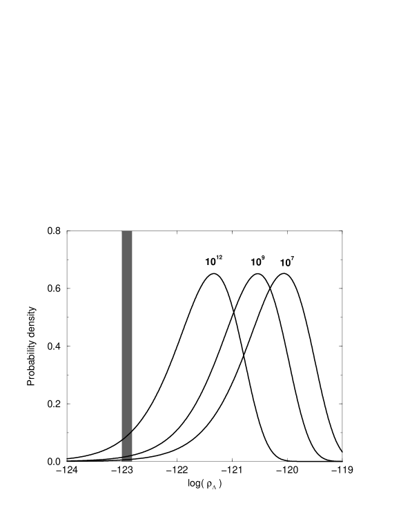
Figure 2: Weighted by “observers per baryon”, the probability distribution for $\rho_{\Lambda}$ depends strongly on specific assumptions about conditions necessary for life. Three curves are shown, corresponding to different choices for the minimum required mass of a galaxy: $M_{*}=(10^{7},10^{9},10^{12})M_{\odot}$. In neither case is the observed value (vertical bar) in the preferred range. The choice $M_{*}=10^{7}M_{\odot}$ (also shown in Fig. 1) corresponds to the smallest observed galaxies. The choice $M_{*}=10^{12}M_{\odot}$ minimizes the discrepancy with observation but amounts to assuming that only the largest galaxies can host observers. By contrast, the Causal Entropic Principle does not assume that observers require structure formation, let alone galaxies of a certain mass; yet its prediction is in excellent agreement with the observed value (see Fig. 8).

Figure 2 shows probability distributions for $\rho_{\Lambda}$, under various assumptions for $M_{*}$. Dwarf galaxies as small as $M_{*}\sim 10^{7}M_{\odot}$ have been detected. With this choice, the observed value of $\Lambda$ is nearly three orders of magnitude, or 3.5$\sigma$, below the median value.

There is some evidence that galaxies with mass below $10^{9}M_{\odot}$ will not retain the heavy elements produced in supernova explosions [25]. Under the additional assumption that such elements are required for life, one may then set $M_{*}$ to this larger value. But the resulting prediction remains unsatisfactory. The median exceeds the observed value by a factor of more than two orders of magnitude, or 2.9$\sigma$.

One can speculate that for some reason, life requires a galaxy as large as our own, or perhaps even a larger group [22, 25] ($M_{*}=10^{12}M_{\odot}$). Then the observed value is about $1.8\sigma$, or a factor of $22$, below the median of the predicted distribution. However, at present we can see no compelling arguments for this extreme choice. Thus, the weighting by observers-per-baryon leads to a dilemma: Either it requires overly specific and questionable assumptions, or else it faces a real conflict with the data.

As these difficulties demonstrate, weighting by observers-per-baryon may not be the correct way to compute probabilities in the landscape. We will now argue for a different approach, which is always well-defined. It will allow us to assume nothing more about observers than that they respect the laws of thermodynamics.

2.3 Weighting by entropy production in the causal diamond

Causal Entropic Principle

In this paper we will compute the probability distribution for $\rho_{\Lambda}$ based on the Causal Entropic Principle, which is defined by the following two conjectures [21]:

• The universe consists of one causally connected region, or “causal diamond”. Larger regions cannot be probed and should not be considered part of the semi-classical geometry.

• The number of observations is proportional to $\Delta S$, the total entropy production in the causal diamond.

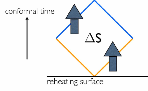
Figure 3: A causal diamond is the largest spacetime region over which matter can interact. It is delimited by a future lightcone from a point on the reheating surface (orange/light), and by a past lightcone from a late-time event (blue/dark); in the case of de Sitter vacua this is the cosmological horizon. A vacuum should be weighted by the number of observations made in this spacetime region. Since observation requires free energy, we expect that on average, this number will be proportional to the amount of entropy, $\Delta S$, produced in the causal diamond. Entropy entering through the bottom cone (bottom arrow), such as the CMB, does not contribute to this entropy difference.

Before motivating the two conjectures, let us first clarify the key terms—causal diamond and entropy—they refer to.

The causal diamond [29] is the largest region of spacetime causally accessible to a single observer. It is defined by the intersection of the past light-cone of a late-time point on the worldline with a future light-cone of an early-time point, shown in Fig. 3. We choose this time to be the time of reheating, since no matter existed before then. (In vacua with no reheating, $\Delta S$ vanishes independently of the choice of the causal diamond. This case does not arise here, since we are holding all parameters other than $\rho_{\Lambda}$ fixed.) Only after reheating can matter begin to interact and commence the formation of complex structures, at most at the speed of light.

In a vacuum with negative cosmological constant, the tip of the top cone would be on the big crunch. In any metastable vacuum with positive cosmological constant, like ours, the top cone is given by the de Sitter event horizon.

One may question the universality of “reheating surface” or our use of an event horizon (a global concept) in a vacuum with finite lifetime, so let us give a more careful definition. A causal diamond can be triggered (that is, a bottom cone drawn) as soon as there is entropy in the matter sector. Reheating is a special case: during inflation, all entropy is in the gravitational sector (the growing horizon of the inflationary universe), but reheating generates matter entropy (mostly radiation, which we include in this class). After vacuum domination in a metastable de Sitter region, the diamond empties out at an exponential rate. If we enlarge the diamond by choosing a later point for the tip, and the additional spacetime volume contains no matter (which will be generic at late times), there is no point in going further. The total amount of matter enclosed by the top cone will be the same as if the vacuum had been completely stable. Once the metastable vacuum decays, reheating may again occur, in which case a new diamond is triggered. This definition implies that if a decay or phase transition happens while there is still matter around, the two vacua should not be considered separate, and a single causal diamond will enclose both. Thus, we are fundamentally defining the range of a causal diamond in terms of the presence of excitations in the matter sector. This is well-defined in the entire regime of semi-classical gravity, independently of the details of the particle physics.

In a de Sitter vacuum, the cosmological horizon has entropy given by one quarter of its surface area. The relevant area is the cross-section of the top-cone of the causal diamond, which grows as matter crosses the horizon. This production of Bekenstein-Hawking entropy would contribute enormously to $\Delta S$. However, it is difficult to see the relevance of horizon entropy to the existence of observers. For the same reason, we will ignore the Bekenstein-Hawking entropy produced in black hole formation. This is also natural since we have defined the causal diamond through this distinction. As we have emphasized above, horizons are a gravitational phenomenon and can always be distinguished from the matter sector in the semiclassical regime. Hence, this restriction does not affect the universality of our method.

To summarize, we will consider exclusively the production of entropy in ordinary matter. We will weight a vacuum by the total entropy increase in the causal diamond:

$$w=\Delta S~{}.$$ (9)

Motivation

From a pragmatic point of view, one can simply regard this proposal as an attractive alternative to weighting by observers-per-baryon. The causal diamond is defined independently of low-energy physics, and the entropy increase is a well-defined quantity that replaces more specific assumptions about observers. However, there are additional, more fundamental reasons to embrace the Causal Entropic Principle. Let us discuss each of the two conjectures put forward at the beginning of this subsection.

The first conjecture is motivated by the study of black holes (see [29, 21, 30] for details). There is now considerable evidence that black hole formation and evaporation is a unitary process [31, 32]. This means that there will be two copies of the initial state at the same instant of time, one inside the black hole, and the other in the Hawking radiation outside. This would appear to violate the linearity of quantum mechanics. However, no actual observer can verify the problem [33, 34], since the two copies reside in causally disconnected regions of the spacetime. Hence, we can escape from the apparent paradox by abandoning the global viewpoint, and be content with merely predicting the observations of (any) one observer.

However, it would be unnatural for such a radical revision of our view of spacetime to be confined to the context of black holes. In many cosmological solutions, a single observer can access only a small portion of the global spacetime. Hence, it is equally important to restrict our attention to only one (cosmological) observer at a time, which is what we do in this paper. Descriptions of cosmology from the local viewpoint can be found, for example, in Refs. [35, 29, 36, 37, 38]. Its implications for eternal inflation were studied in Ref. [39].

The second conjecture replaces far more specific conditions assumed to be necessary for observers, such as the existence of galaxies, stable planetary orbits, suitable chemistry, etc., which were needed in the observers-per-baryon approach. The basic idea is that observers, whatever their form, have to obey the laws of thermodynamics. Observation requires free energy and is clearly incompatible with thermal equilibrium or an empty universe. The free energy, divided by the temperature at which it is radiated, can be regarded as a measure of the potential complexity arising in a spacetime region. This is equal to the number of quanta produced, or more fundamentally, the entropy increase $\Delta S$.

It seems plausible that there might be an absolute minimum complexity necessary for observers, so that subcritical weights $\Delta S<\Delta S_{\rm crit}$ should be replaced by zero. For example, it seems likely that vacua with $\rho_{\Lambda}$ of order unity, which can contain only a few bits, have strictly zero probability of hosting observers (see also Ref. [40]). However, any such cutoff does not appear to play an important role for the questions studied here. We choose the weight factor to be simply $\Delta S$, with no cutoff.

To avoid confusion, we stress that our weighting has nothing to do with the Hartle-Hawking amplitude, $\exp(S_{\rm dS})$, which describes the number of quantum states associated with a de Sitter horizon [41]. The number of observers, and of observations, is naturally proportional to an entropy difference, $\Delta S$, not to an absolute entropy or the exponential of an entropy. (Despite our appropriation of the term “entropic principle”, for which we apologize to the authors, there is also little relation to Ref. [42].)

We could have adopted only the first conjecture, and continued to estimate the number of observers by more explicit anthropic criteria. This would not have changed our final result significantly. But why make a strong assumption if a more conservative one suffices? Our results suggest that the poor predictions from weighting by observers-per-baryon stemmed not from a lack of specificity in characterizing observers, but from the regularization scheme (“per baryon”). The causal diamond cutoff solves this problem, and allows us to weaken anthropic assumptions to the level of an inevitable thermodynamic condition.

Moreover, $\Delta S$ is a well-defined weight in any vacuum, however different from ours. It will be a powerful tool in future work, when parameters other than $\rho_{\Lambda}$ are allowed to vary simultaneously. We are thus motivated to use our second conjecture throughout. We will find that in our own universe, it captures conditions for observers remarkably well.

3 Computing $\rho_{\Lambda}$ from the Causal Entropic Principle

In this section, we will compute the probability distribution over $\rho_{\Lambda}$, holding all other physical parameters fixed. We do this in four steps. First, we will compute the geometry of the causal diamond as a function of $\rho_{\Lambda}$. Next, we will identify important effects that produce entropy within the causal diamond. Then we will determine the time-dependence of the entropy production rate per unit comoving volume, as a function of $\rho_{\Lambda}$. Finally, we will fold this together with the time-dependence of the comoving volume contained in the causal diamond to obtain the weight factor, $\Delta S(\rho_{\Lambda})$.

3.1 Metric and causal diamond

Current data are consistent with a spatially flat universe. Hence, we will assume that since the time of reheating, the large scale structure of our universe is described by a spatially flat FRW model:

$$ds^{2}=-dt^{2}+a(t)^{2}d{\mathbf{x}}^{2}~{}.$$ (10)

(Actually, we are making the stronger assumption that the cosmological constant dominates before curvature does, for all values of $\rho_{\Lambda}$ considered here. Thus, we are assuming that the universe is flatter than necessarily required by current constraints.)

After reheating, the universe will be dominated first by radiation, then by matter, and finally by vacuum energy. The reheating temperature will not be important; in fact, we will neglect the radiation era altogether. Instead, we extrapolate the matter-dominated era all the way back to the big bang ($t=0$), where we will place the bottom tip of the causal diamond. This approximation is justified because the radiation era contributes only a small fraction of conformal time in the range of values of $\rho_{\Lambda}$ that have any significant probability. This is shown in detail in Appendix A.

Thus, we treat the universe as containing only pressureless matter and a cosmological constant. At early times (matter domination), the scale factor will be proportional to $t^{2/3}$, independently of $\rho_{\Lambda}$. At late times (vacuum domination) it will grow like $\exp(t/t_{\Lambda})$, where

$$t_{\Lambda}=\sqrt{\frac{3}{\Lambda}}=\sqrt{\frac{3}{8\pi\rho_{\Lambda}}}~{},$$ (11)

(In our universe, with $\rho_{\Lambda}$ given by Eq. (1), we have $t_{\Lambda}\approx 0.98\times 10^{61}=16.7$ Gyr).

An exact solution (aside from the neglected radiation era) that includes both regimes is

$$a(t) = \left[t_{\Lambda}\sinh\left(\frac{3}{2}\frac{t}{t_{\Lambda}}\right)\right]^{2/3}\,,$$ (12)

$$\rho(t) = \rho_{\Lambda}+\rho_{\rm m}=\rho_{\Lambda}\left[1+\frac{1}{\sinh^{2}\left(\frac{3}{2}\frac{t}{t_{\Lambda}}\right)}\right]~{}.$$ (13)

The prefactor, $t_{\Lambda}^{2/3}$, is arbitrary and can be changed by rescaling the spatial coordinates. Our choice ensures that for solutions with different values of $\Lambda$, the scale factors will agree at early times not only by diffeomorphism, but explicitly. This is convenient because $\Lambda$ is dynamically irrelevant at early times.

Vacuum energy begins to dominate the density when $\rho_{\Lambda}=\rho_{\rm m}$, at $t=0.59\,t_{\Lambda}$ (in our universe, 9.8 Gyr after the big bang). Acceleration begins earlier, when $\rho+3p=\rho_{\rm m}-2\rho_{\Lambda}=0$, at $0.44\,t_{\Lambda}$ (in our universe, at 7.3 Gyr).

In order to compute the boundaries of the causal diamond, it is convenient to work in conformal time, $\tau=\int dt/a(t)$. The metric becomes

$$ds^{2}=a(\tau)^{2}[-d\tau^{2}+d{\mathbf{x}}^{2}]~{}.$$ (14)

Light-rays obey $ds=0$, and hence for radial light-rays, $d\tau=\pm dr$, where $r=|{\mathbf{x}}|$.

Using our solution, Eq. (12), conformal time will be given by

$$\tau(t) = -t_{\Lambda}^{1/3}\frac{1}{\cosh^{2/3}\left(\frac{3t}{2t_{\Lambda}}\right)}F\left(\frac{5}{6},\frac{1}{3},\frac{4}{3},\frac{1}{\cosh^{2}\left(\frac{3t}{2t_{\Lambda}}\right)}\right)$$ (15)

$$= -\frac{t_{\Lambda}}{a(t)}F\left(\frac{1}{3},\frac{1}{2},\frac{4}{3},\frac{-t_{\Lambda}^{2}}{a(t)^{3}}\right)\,.$$ (16)

It has finite range, running from

$$\tau(0)=-\frac{\Gamma(\frac{4}{3})\Gamma(\frac{1}{6})}{\Gamma(\frac{1}{2})}t_{\Lambda}^{1/3}\approx-2.804\,t_{\Lambda}^{1/3}$$ (17)

at the big bang, to $\tau(\infty)=0$ at asymptotically late times. The total conformal lifetime of the universe is $\Delta\tau=\tau(\infty)-\tau(0)=2.804\,t_{\Lambda}^{1/3}$.

The causal diamond is given by the region delimited by

$$r=\frac{\Delta\tau}{2}-\left|\frac{\Delta\tau}{2}+\tau\right|~{}.$$ (18)

The comoving volume inside the causal diamond at conformal time $\tau$ is simply

$$V_{\rm c}=\frac{4\pi}{3}r^{3}(\tau)\,.$$ (19)

This is shown in Fig. 4, as a function of proper time,

Figure 4: The lower plot shows comoving volume in the causal diamond, $V_{\rm c}$, as a function of time for $\rho_{\Lambda}=(0.1,1,10)$ times the observed value given in Eq. (1). The kink in the comoving volume corresponds to the “edge” of the causal diamond, where the top and bottom cone meet (see Fig. 3). The upper plot shows the rate of entropy production computed in Sec. 3.3, which peaks around 2 to 3.5 Gyr. As explained in Sec. 4.2, the Causal Entropic Principle prefers values of $\rho_{\Lambda}$ such that the ($\rho_{\Lambda}$-dependent) peak of the comoving volume coincides with the (nearly $\rho_{\Lambda}$-independent) peak of the entropy production rate (see Fig. 9.

for several values of $\rho_{\Lambda}$. The maximum comoving volume occurs at the edge of the causal diamond at conformal time $\tau(0)/2$, or equivalently,

$$t_{\rm edge}\approx 0.23t_{\Lambda}$$ (20)

(in our universe, $t_{\rm edge}\approx 3.9$ Gyr). The maximum comoving volume itself is $V_{\rm c}(\tau(0)/2)\approx 11.6t_{\Lambda}$.

At late times, the comoving volume goes to zero. This reflects the exponential dilution of all matter, which is expelled from the diamond by the accelerated expansion. The physical radius approaches a constant, $t_{\Lambda}$, the horizon radius of the asymptotic de Sitter space. Note that the “comoving four-volume”,

$$V_{4}\equiv\int_{0}^{\infty}V_{\rm c}(t)dt~{},$$ (21)

is finite. It is proportional to $t_{\Lambda}^{2}$, and hence, inversely proportional to the cosmological constant. This will be important, since it means that smaller values of $\rho_{\Lambda}$ are rewarded by a larger causal diamond, and thus, potentially greater complexity. This can compensate for their rarity.

3.2 Major sources of entropy production

To calculate $dP/d(\log\rho_{\Lambda})$, we need to calculate the total entropy production in the causal diamond as a function of the cosmological constant, $\Delta S(\rho_{\Lambda})$. We have determined above how the causal diamond depends on $\rho_{\Lambda}$, but we must also understand how the rate of entropy production depends on $\rho_{\Lambda}$. We begin by identifying the major sources contributing to $\Delta S$ in the causal diamond in our own vacuum.

First, let us discuss sources which can be neglected. Because the causal diamond is small at early times ($\frac{\tau}{\tau_{\infty}}\ll 1$), and empty at late times ($1-\frac{\tau}{\tau_{\infty}}\ll 1$), the most important contributions will be produced in the era between 0.1 Gyr to 100 Gyr, when the comoving volume shown in Fig. 4 is large. Hence, we can disregard the entropy produced at reheating, at phase transitions, or by any other processes in the early universe. Virtually all of this entropy (in particular, the cosmic microwave background) entered the causal diamond through the bottom cone and does not contribute to $\Delta S$.

For the same reason, we neglect the entropy in Hawking radiation produced by supermassive black holes. (One might contemplate the possibility of a “planet” orbiting such an object and exploiting its very low temperature radiation as a source of free energy.) However, the timescale for the evaporation of a black hole is enormous ($M^{3}$). By the time this entropy would be produced, a typical causal diamond, on which the measure for prior probabilities is based in the local approach [21], will be completely empty.

Having dismissed effects at small comoving volume, we turn to processes which operate from 0.1 Gyr to 100 Gyr, when the comoving volume is large. In this era, entropy is produced by baryonic systems, and we can gauge the importance of a given process by its total entropy production per baryon, or equivalently, per unit mass, or unit comoving volume, $dS/dV_{\rm c}$. This can be estimated as the ratio between the amount of energy released per baryon, and the temperature at which this energy is dominantly radiated.

Stars

Ten percent of baryons end up in galaxies, and thus in stars. Approximately ten percent of those baryons actually burn in the course of the lifetime of the star. The energy released is about 7 MeV for each baryon in the reaction 4p $\rightarrow$ ⁴He, or about $0.7\times 10^{-2}$ of the rest mass of the proton. Stars radiate at varying temperatures corresponding largely to optical wavelengths (about 0.2 to 3 eV). However, more than half of this radiation is reprocessed by dust [43]. It is re-emitted in the infrared, at approximately $60\,\mu$m, or $20$ meV. Hence, there will be more than 100 infrared photons per optical photon [44], and the infrared emission will dominate the entropy production. In summary, stellar burning produces an entropy of order $10^{6}$ per baryon, after reprocessing by dust.

Active galactic nuclei

Active galactic nuclei (AGNs) appear to be the main competitor to stars in terms of luminosity and entropy production. Approximately $10^{-3}$ of the total stellar mass (i.e., $10^{-4}$ of baryonic mass) ends up in supermassive black holes, and perhaps 10% of this energy is released during the violent accretion process. This suggests that AGNs release at most about one sixth of the energy as compared with stellar burning. The effective temperature will again be 20 meV, since a large fraction of the radiation is reprocessed by dust. Hence, AGNs appear to produce somewhat less total entropy per baryon than stars, and we will neglect their contribution in the present paper.

In Ref. [45], the intrinsic luminosities of all AGNs above observational limits were compiled to create a quasar luminosity function applicable back to about 1 Gyr after the big bang. This luminosity function suggests that the entropy production rate from quasars is more narrowly peaked than that estimated for stars in Fig. 6. But even at the peak, near a redshift of $z=2$, the quasar luminosity is a factor of 3 lower than the present stellar luminosity [46] (which, in turn, is about one order of magnitude lower than the peak stellar luminosity). This seems to rule out the possibility that AGNs ever dominated the entropy production rate.

Other potentially important contributions come from galaxy cooling and from supernovae. Even assuming reprocessing by dust, neither of these phenomena can compete with stellar burning, because they run on less energy but not at lower temperature.

Supernovae

We focus on core collapse supernovae since they are more abundant than type Ia supernovae (by factor of 4-5) while producing comparable luminosity per event. They occur in all stars with more than eight solar masses, which constitute 1% of the total stellar mass [see Eq. (26)]. The collapse of an iron core into a neutron star releases gravitational binding energy not much smaller than the core mass (1.4 solar masses). Thus roughly 10% of the total mass of the progenitor is released. Most of this energy is carried away by high energy neutrinos, producing little entropy. Only 1% produces optical photons, and is reprocessed by dust into infrared photons. Altogether, supernovae thus convert a fraction of $10^{-5}$ of stellar baryonic mass into soft photons.

Further quantitative analysis confirms the above estimate. We find that entropy production from supernovae is more than order of magnitude below the contribution from dust heated by stars.

Galaxy cooling

A typical galaxy like ours has a mass-to-radius fraction of approximately $10^{-6}$. This fraction of the galaxy mass is converted into kinetic energy at virialization. This energy, about $1$ keV per stellar baryon, is converted into radiation as the galaxy cools. The virial temperature is about $10^{5}$ K, or 10 to 100 times greater than the temperature of a star. Even assuming reprocessing by dust, galaxy cooling will produce less than $10^{4}$ photons per baryon. This is more than two orders of magnitude below the entropy production from dust heated by stars.

3.3 Entropy production rate

We have argued that the dominant source of entropy production in our universe is dust heated by starlight. In this subsection we will consider the rate at which this entropy is produced. We will ask how it depends on time and on $\rho_{\Lambda}$.

Time dependence

Deriving $dS/dV_{\rm c}\,dt$ from first principles would require a detailed description of all of the dynamics that led up to stellar burning, such as non-linear evolution, gas cooling and disk fragmentation. Instead, we will take advantage of observations that quantify the time-dependence of the star formation rate. This will allow us to obtain the entropy production from dust heated by stars. We will then estimate how this rate changes in universes with different cosmological constants. Surprisingly, this latter dependence will not be important for our final result.

In recent years, observations of the extragalactic background radiation in a large range of wavelengths have improved our understanding of the galaxy luminosity function. This has allowed astronomers to infer the star formation rate (SFR) in galaxies, and its evolution in time [47, 48] (see [49] for a review). The SFR is defined as the rate of stellar mass production per comoving volume

$$\dot{\rho}_{\star}(t)\equiv\frac{\partial^{2}M_{\star}}{\partial V_{\rm c}\partial t}\,.$$ (22)

This function is constrained by observation through a variety of techniques. For example, UV emission from star-forming galaxies is dominated by massive stars that are short-lived. Due to the short lifetime, luminosities in these wavelengths track the birth rate of stars [50]. In addition, detailed surveys of the local universe constrain the SFR at low redshift [51, 52]. Bounds on the rate of type II supernovae from Super-Kamiokande and KamLAND also place an indirect bound on stellar birth [53].

The combination of these measurements constrain the SFR back to redshifts of about $z\sim 6$, when the universe was 1 Gyr old. Since then, the SFR may be grossly described as a smooth function that peaks at around 2.5 Gyr and subsequently decreases exponentially with time. The SFR today is roughly one order of magnitude less than its peak value. As we shall see, the era of peak stellar formation, which we will call $t_{\star}$, will play an essential role in determining the cosmological constant using the Causal Entropic Principle.

Several authors have postulated models or functional forms for the SFR, fitting model parameters to the data, for example [54, 55, 56, 57]. Variations between the fits lead to a range for $t_{\star}\sim 1.5-3$ Gyr.

We will illustrate our computation using two different SFRs, in order to illustrate the systematic dependence of our calculation on the time dependence of star formation. The first SFR is from Ref. [56] (labeled “N” in plots) and has $t_{\star}\sim 1.7$ Gyr. The second SFR, from Ref. [57] (labeled “H”), peaks at $t_{\star}\sim 2.8$ Gyr. We will find in both cases that the observed value of $\rho_{\Lambda}$ lies well inside the $1\sigma$ region of the resulting probability distribution.

Figure 5: The star formation rate as a function of time from Nagamine et al. [56], labeled “N”, and from Hopkins and Beacom [57], labeled “H”. They are peaked at $t_{\star}\sim$1.7 Gyr and 2.8 Gyr respectively. We have normalized both SFRs such that the stellar luminosity density calculated below agrees with the bolometric luminosity observed today. It should be noted, however, that our result is not sensitive to this re-normalization.

Both SFRs are shown in Fig. 5 re-normalized. One of the biggest uncertainties regarding the determination of the star formation rate is the overall normalization of the curve. Fortunately our result is completely insensitive to this overall normalization; it depends only on the shape of the SFR.

For concreteness, we have normalized the SFR such that the implied stellar luminosity today matches the observed bolometric luminosity from low-redshift stars, $10^{8.6}L_{\odot}/\mathrm{Mpc}^{3}$. Our normalizations differs from those in the original works since we have used rather rudimentary formulae to compute the present luminosity from the SFR. However, the shape of the total entropy production rate derived with these simple formulae agrees well with that in Ref. [56] when this SFR is used.

With the rate of star formation in hand, one can estimate the rate of entropy production by stars. Let us first consider a single star of mass $M$ born at a time $t^{\prime}$. Its entropy production rate is the stellar luminosity divided by the temperature at which photons are radiated,

$$\frac{d^{2}s}{dN_{\star}dt}(M)=\frac{L_{\star}}{T_{\rm eff}}\sim\frac{1}{2}\left(\frac{M}{M_{\odot}}\right)^{3.5}\frac{L_{\odot}}{20\,\mathrm{meV}}=\frac{1}{2}\left(\frac{M}{M_{\odot}}\right)^{3.5}3.7\times 10^{54}\ \mathrm{yr}^{-1}\,.$$ (23)

Here we have assumed a mass-luminosity relation

$$L_{\star}\propto M^{3.5}\,.$$ (24)

(We use $M_{\star}$ to refer to total stellar mass, and $M$ to refer to the mass of a specific star. $N_{\star}$ denotes star number.) The effective temperature of 20 meV is that of the dust which reprocesses about one half (hence the prefactor) of the starlight and dominates photon number.

The star will only produce entropy over a finite time $t_{\star}$ that also depends on $M$:

$$t_{\star}(M)\sim\left(\frac{M_{\odot}}{M}\right)^{2.5}10^{10}\;\mathrm{yr}.$$ (25)

Now let us consider a whole population of stars that are formed at a time $t^{\prime}$. At birth, stellar masses are observed to be distributed according to a universal, time-independent function known as the initial mass function (IMF). The Salpeter distribution [58], which goes as $M^{-2.35}$, agrees reasonably with observation, but has since been refined by many authors. In the present calculation we will use a modified Salpeter IMF of the form [57]

$$\xi_{\mathrm{IMF}}(M)\equiv\frac{dN_{\star}}{dM}=\left\{\begin{array}[]{ll}C_{1}M^{-2.35}&\mbox{for}\ M\geq 0.5M_{\odot}\\ C_{2}M^{-1.5}&\mbox{for}\ M<0.5M_{\odot}\end{array}\right.~{},$$ (26)

where the constants $C_{1,2}$ are set by requiring that the IMF is continuous and that it integrate to one over the range $0.08M_{\odot}<M<100M_{\odot}$.

We now have all the ingredients in place to calculate $d^{2}S/(dM_{\star}dt)$, the contribution of a stellar population that is born at time $t^{\prime}$ to the entropy production rate at some later time $t>t^{\prime}$, per unit initial stellar mass. This rate is a function only of the time difference $t-t^{\prime}$

$$\frac{d^{2}S}{dM_{\star}dt}(t-t^{\prime})=\frac{1}{\langle M\rangle}\int_{M_{\mathrm{min}}}^{M_{\mathrm{max}}(t-t^{\prime})}dM\,\xi_{\mathrm{IMF}}\frac{d^{2}s}{dN_{\star}dt}(M)~{},$$ (27)

with the average initial mass (defined at $t^{\prime}$), $\langle M\rangle$, defined as

$$\langle M\rangle=\int_{0.08M_{\odot}}^{100M_{\odot}}dM\,\xi_{\mathrm{IMF}}M\approx 0.48M_{\odot}~{}.$$ (28)

The time dependence enters Eq. (27) through the death of stars of various masses at different times and thus appears in the upper limit of the upper integral. It is derived by inverting equation (25):

$$M_{\mathrm{max}}(t-t^{\prime})=\left\{\begin{array}[]{ll}100M_{\odot}&\ \mbox{for}\ t-t^{\prime}<10^{5}\ \mbox{yr}\\ \left(\frac{10^{10}\;\mathrm{yr}}{t-t^{\prime}}\right)^{2/5}M_{\odot}&\ \mbox{for}\ t-t^{\prime}>10^{5}\ \mbox{yr}\\ \end{array}\right.\,.$$ (29)

The lower limit of the integral is set by the minimal mass of stars that can sustain nuclear burning,

$$M_{\mathrm{min}}=0.08M_{\odot}\,.$$ (30)

These stars burn for $\sim 5000$ Gyr, living well into vacuum domination in our universe.

Figure 6: The entropy production rate in our universe as a function of time, from dust heated by starlight. The two curves shown correspond to different models of the star formation history of the universe [56, 57]; see Fig. 5.

In order to calculate the entropy production rate in the universe at time $t$ we must convolve $d^{2}S/(dM_{\star}dt)$ with the SFR. That is, we integrate over the birth times $t^{\prime}$ of all populations of stars born before the time $t$:

$$\frac{d^{2}S}{dV_{\rm c}dt}(t) = \int_{0}^{t}dt^{\prime}\,\frac{d^{2}S}{dM_{\star}dt}(t-t^{\prime})\frac{d^{2}M_{\star}}{dV_{\rm c}dt^{\prime}}(t^{\prime})$$ (31)

$$= \int_{0}^{t}dt^{\prime}\,\frac{d^{2}S}{dM_{\star}dt}(t-t^{\prime})\,\dot{\rho}_{\star}(t^{\prime})\,.$$

This function is plotted in Fig. 6 for the two forms of the SFR. It is a smooth function that peaks when the universe is about 2.3 Gyr old and 3.3 Gyr old for the two curves plotted. This timescale is set by the peak of the star formation rate and the mean lifetime of a star in our universe. The entropy production rate decreases as stars born during the peak of the SFR begin to die. But due to the high abundance of long-lived low mass stars, $\partial_{V_{\rm c}}\dot{S}$ maintains a finite value long after star formation has ceased.

In our approximation, the entropy production rate is half the luminosity of stars at the time $t$, divided by the effective temperature (dust at 20 meV). Modulo this rescaling, Fig. 6 thus also shows our estimate for the luminosity, which was used for normalization as described above.

We caution that we assumed overly simplistic formulae for the luminosity and the lifetime of a star. For example, we ignored the dependence on metallicity, and a dependence of the exponent in Eq. (24) on the mass. This will likely affect the shape of the entropy production rate somewhat, as will corrections from other sources of entropy. However, our prediction for $\rho_{\Lambda}$ depends only on the roughest features: the width and position of the peak of the entropy production rate. Hence, it is unlikely that our result would be qualitatively affected by our simplifications.

Dependence on $\rho_{\Lambda}$

The entropy production rate calculated above is that in our universe. In order to determine $\Delta S(\rho_{\Lambda})$, we will need to calculate this function for universes with different values of the cosmological constant. Interestingly, this dependence will be of little importance for our final result.

Stars have decoupled from the global expansion of the universe, so their internal dynamics is unaffected by variations of $\rho_{\Lambda}$. However, the value of $\rho_{\Lambda}$ affects the fraction of baryons that are incorporated in halos large enough to form stars at any given time, thus affecting the star formation rate, and ultimately the entropy production. For example, if $\rho_{\Lambda}$ is large enough to violate Weinberg’s anthropic bound, no baryons will be in star forming halos and $\Delta S$ will be very suppressed.

In a universe with a vacuum energy density $\rho_{\Lambda}$, the fraction of matter that is incorporated in halos of a mass $M_{G}$ by time $t$ or above, $F(\rho_{\Lambda},M_{G},t)$, is easily calculated in the Press-Schechter (PS) formalism [59]. The formulae for the PS fraction are summarized in [4]. (This fraction is also a function of the amplitude of density perturbations and the temperature at matter-radiation equality, but since these are held fixed in this calculation we will suppress them.)

For the purpose of our calculation, we will consider a galaxy to be star-producing if the mass of its host halo is $10^{7}M_{\odot}$ or above. Note that this choice involves no speculation about what observers need. The Causal Entropic Principle requires us to compute the entropy production rate as a function of $\rho_{\Lambda}$. This rate depends on whether or not stars, the dominant contributors of entropy, actually form. For $M_{G}>10^{7}M_{\odot}$, the virial temperature of the halo is above $10^{3}$ K, enough to support rapid line cooling and efficient stellar production. (The first generation of stars—Population III—were formed in galaxies with even lower masses, but since these stars have been neither observed nor accounted for in the observation-based SFRs, we will not consider them further.) In any case, as we shall see, our final result will be quite insensitive to this choice.

Based on the SFR $\dot{\rho}_{\star}(t)$ in our universe, we will now estimate the SFR in a universe with a different vacuum energy, $\dot{\rho}_{\star}(\rho_{\Lambda},t)$. The SFR in our universe is peaked at about $t_{\star}\sim 1.5-3$ Gyr, which is still in the matter dominated era. The cosmological constant played no dynamical role and cannot have anything to do with this peak. Rather, this time scale is set by astrophysical dynamics, such as galaxy formation, cooling, and feedback.

Figure 7: The entropy production rate of Fig. 6 depends only mildly on the vacuum energy. Hence, dependence on the vacuum energy enters our calculation mainly through the size of the causal diamond (see Figures 4 and 9). The rate of Ref. [56] is shown here for $\rho_{\Lambda}=(0.1,1,10)$ times the observed value (from top to bottom) using the approximation of equation 32.

Therefore, the star formation rate depends mainly on the mass fraction in star forming galaxies at the critical time $t_{\star}$. Strictly speaking, the SFR will be sensitive to the PS fraction at times before $t_{\star}$ because of the cooling period that is required between the time a baryonic structure goes non-linear and the time it collapses into stars. Baryons that burn during the peak of the SFR actually fell into non-linear halos a cooling time earlier. We leave a more careful analysis of these and other effects to further investigation.

Let us define $F_{\star}(\rho_{\Lambda})$ as the PS fraction that is most relevant for star formation in a universe with cosmological constant $\rho_{\Lambda}$, namely that evaluated at $t_{\star}$, with a minimum mass of $10^{7}M_{\odot}$. In order to capture the mild sensitivity of the SFR to changes of the cosmological constant, we rescale the SFR by the appropriate $F_{\star}$:

$$\dot{\rho}_{\star}(\rho_{\Lambda},t)=\dot{\rho}_{\star}(t)\times\frac{F_{\star}(\rho_{\Lambda})}{F_{\star}(1.25\times 10^{-123})}\,.$$ (32)

Because the observed value of $\rho_{\Lambda}$ is far from disturbing the formation of $10^{7}M_{\odot}$ galaxies, small variations of $\rho_{\Lambda}$ will barely affect the mass fraction $F_{\star}$; see Fig. 7. But they do affect the geometry of the causal diamond. This is the reason why the latter effect will be important for our final result, while Eq. (32) gives only a tiny correction.

3.4 Total entropy production in the causal diamond

From the above results, we can compute the total entropy production

$$\Delta S(\rho_{\Lambda})=\int_{0}^{\infty}dt\,V_{\rm c}(\rho_{\Lambda},t)\partial_{V_{\rm c}}\dot{S}(\rho_{\Lambda},t)~{}.$$ (33)

Here, $V_{\rm c}$ is the comoving volume in the causal diamond at the time $t$, given in Eq. (19). $\partial_{V_{\rm c}}\dot{S}$ is the rate of entropy production per unit comoving volume, given in Eq. (31). The dependence on $\rho_{\Lambda}$ enters mainly through $V_{\rm c}$. It is straightforward to perform the integrals numerically.

By Eqs. (8) and (9), the probability distribution $dP/d(\log\rho_{\Lambda})$ is proportional to $\rho_{\Lambda}\Delta S(\rho_{\Lambda})$. We show this distribution in Fig. 8 for both the Nagamine et al. [56] as well as the Hopkins et al. [57] SFRs.

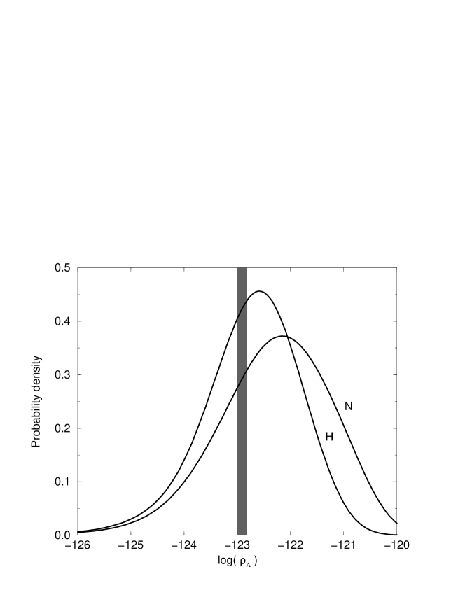
Figure 8: The probability distribution over $\log(\rho_{\Lambda})$ computed from the Causal Entropic Principle. The two curves shown arise from two different models of the star formation rate (see Figs. 5 and 6). Their differences hint at the systematic uncertainties in our calculation that arise since the history of entropy production is not known to arbitrary precision. These uncertainties are apparently irrelevant to our main conclusion: either way, the observed value of $\rho_{\Lambda}$ (vertical bar) is not unlikely.

For the Nagamine et al. SFR, the median value is $\rho_{\Lambda}=5.6\times 10^{-123}$ with the $1\sigma$ error band between $4.2\times 10^{-124}$ to $5.8\times 10^{-122}$. For the Hopkins et al. SFR, we find the median value $\rho_{\Lambda}=2.1\times 10^{-123}$ with the $1\sigma$ error band between $2.4\times 10^{-124}$ to $1.4\times 10^{-122}$.

There are “systematic uncertainties” in our calculation of the probability distribution, which come from our lack of knowledge of the precise history of entropy production in our universe. The comparison between the two models for the SFR gives a good sense of their size. It shows that these uncertainties do not affect our conclusion: with either choice, the observed value is well within the $1\sigma$ region, and hence, not unlikely.

4 Discussion

4.1 $\Delta S$ captures complexity

Our main quantitative result is the probability distribution for $\rho_{\Lambda}$. However, we have also discovered an important intermediate result: in our own causal diamond, the dominant contribution to entropy production comes from the infrared glow of dust heated by starlight.

This is remarkable. It shows that a seemingly primitive quantity, $\Delta S$, captures many of the conditions that are usually demanded explicitly by anthropic arguments. $\Delta S$ would drop sharply if galaxies, stars, or heavy elements were absent. According to the Causal Entropic Principle, the weight carried by such a vacuum would be suppressed.

For example, consider a universe like ours, except without heavy elements. (This could be arranged by adjustments in the standard model.) Galaxies would still form, and stars would burn, but there would be no dust available to convert optical photons into a much larger number of infrared photons [43]. The Causal Entropic Principle assigns a weight 100 times larger to our vacuum than to this one—simply based on the entropy production, without knowing anything about the potential advantages of heavy elements often claimed in anthropic arguments.

This demonstrates that $\Delta S$ can be an effective and very simple substitute for a number of dubious anthropic conditions. More importantly, our result lends credibility to $\Delta S$ as a weighting factor for vacua with very different low-energy physics. Estimating the number of observers in such vacua, even averaged over a large parameter space, appears wholly intractable, but estimating $\Delta S$ may not be.

Thus, the Causal Entropic Principle may allow us, for the first time, to predict probability distributions over the entire landscape, rather than just over subspaces constrained to coincide with much of our low-energy physics. As discussed in Sec. 1, this could lead to a breakthrough on extracting predictions directly from the underlying theory (the string landscape), without conditioning on parameters specific to our own vacuum.

4.2 Understanding our distribution

Now, let us turn to our main result. In our approach, the most likely range of $\log\rho_{\Lambda}$ is set not by the time of galaxy formation, but by the time at which the rate of entropy production, per unit time and unit comoving volume, is largest. This can be understood as follows.

Consider, for the sake of argument, an entropy production rate that is independent of time and of $\rho_{\Lambda}$. Then the total entropy $\Delta S$ produced within the causal diamond is proportional to $\int V_{\rm c}(t)\,dt$, where $V_{\rm c}$ is the comoving volume (or equivalently, the mass) present inside the causal diamond at the time $t$. This integral is the area under the curves shown in the lower panel of Fig. 4.

At small times (near the bottom tip) the causal diamond is small and $V_{\rm c}$ is negligible. After vacuum domination, at a time of order $t_{\Lambda}=(3/8\pi\rho_{\Lambda})^{1/2}$, the top cone, which contains one de Sitter horizon region, quickly empties out and $M(t)$ vanishes exponentially. Thus, only the era around the time of matter/vacuum equality contributes significantly to the integral.

Up to a $\rho_{\Lambda}$-independent factor of order unity, the above integral is therefore the product of $t_{\Lambda}M(t_{\Lambda})$. But $M(t_{\Lambda})$ is just the total mass inside the horizon around the time when $\Lambda$ begins to dominate. This is again of order $t_{\Lambda}$ and thus proportional to $\rho_{\Lambda}^{-1/2}$. Hence the total entropy produced, $\Delta S$, scales like $1/\rho_{\Lambda}$ in our hypothetical case of a constant entropy production rate. This is also clear by inspecting the area under the different curves in Fig. 4.

Assuming a flat prior ($dp/d\rho_{\Lambda}=\mbox{const}$, or equivalently, $dp/d\log\rho_{\Lambda}\propto\rho_{\Lambda}$), the observer-weighted probability distribution is

$$\frac{dP}{d\log\rho_{\Lambda}}\propto w(\rho_{\Lambda})\rho_{\Lambda}~{},$$ (34)

and the Causal Entropic Principle states that the weight is

$$w=\Delta S~{}.$$ (35)

For the hypothetical, constant entropy production rate, we have $w\propto\rho_{\Lambda}^{-1}$, and hence

$$\frac{dP}{d\log\rho_{\Lambda}}=\mbox{const}~{}.$$ (36)

The weight $\Delta S$ in this case takes a prior distribution that was flat in $\rho_{\Lambda}$ into an observer-weighted distribution that is flat in $\log\rho_{\Lambda}$, showing no preference between, say, $\rho_{\Lambda}=10^{-121}$ and $\rho_{\Lambda}=10^{-123}$.

In the prior distribution, there are more vacua at large $\rho_{\Lambda}$, so exponentially small values of $\rho_{\Lambda}$ are very unlikely. The above example shows that the Causal Entropic Principle captures an important compensating factor: vacua with smaller $\rho_{\Lambda}$ give rise to a larger causal diamond, i.e., to a bigger de Sitter horizon and a longer time until vacuum domination. This allows for greater complexity and compensates for the rarity of such vacua.

Next, let us consider the time-dependent entropy production rate we found in Sec. 3.3. We found that the entropy production due to stars has a fairly broad peak around $t_{\rm peak}\sim 2$ to 3.5 Gyr after the big bang. At earlier times, it is lower because fewer stars have formed; at late times, it is lower because few new stars form while older ones have burned out.

Because of the time dependence, $\rho_{\Lambda}\Delta S$ will no longer be constant. For large values of $\rho_{\Lambda}$, the causal diamond is small, and it will contain only a small comoving volume by the time the entropy production peaks [$t_{\rm peak}\gg t_{\rm edge}=0.23t_{\Lambda}$; see Eq. (20)]. In this regime, $dP/d\log\rho_{\Lambda}$ will decrease with $\rho_{\Lambda}$. For small $\rho_{\Lambda}$, the causal diamond is very large, but the entropy production rate peaks early, when the comoving volume is still relatively small ($t_{\rm peak}\ll t_{\rm edge}$). In this regime, $dP/d\log\rho_{\Lambda}$ will increase with $\rho_{\Lambda}$. This is illustrated in Fig. 9.

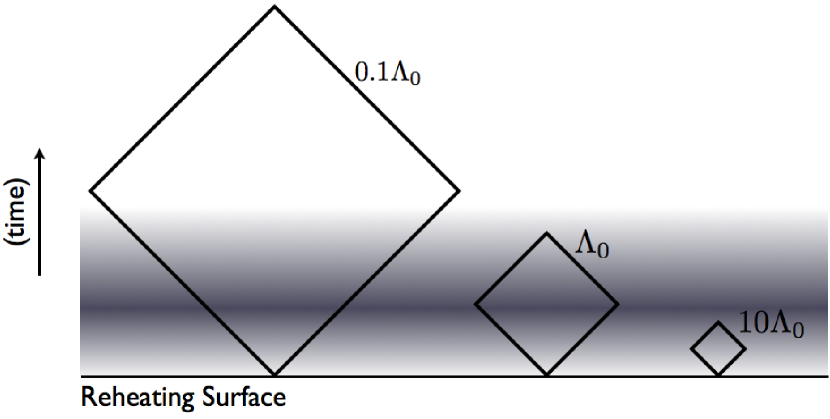
Figure 9: This cartoon demonstrates how the Causal Entropic Principle leads to a preferred value of the cosmological constant. The horizontal band represents the rate of entropy production; darker areas correspond to a higher rate. Vacua are weighted by $\Delta S$, the total amount of “darkness” inside a causal diamond. Vacua with large cosmological constant are plentiful in the landscape, but they lead to small causal diamonds, which capture virtually no entropy production (right). For some smaller value, the diamond will be just large enough to capture the bulk of the entropy production (center). This is the preferred cosmological constant. Larger diamonds may capture slightly more $\Delta S$ (left), but not in proportion to their size. They correspond to vacua with very small cosmological constant which are much rarer in the landscape. Therefore they will be suppressed.

Therefore, $dP/d\log\rho_{\Lambda}$ will be maximal for values of $\rho_{\Lambda}$ such that

$$t_{\rm edge}(\rho_{\Lambda})=t_{\rm peak}~{}.$$ (37)

By Eqs. (11) and (20), the observed value of $\log\rho_{\Lambda}$ should be near

$$\log\rho_{\Lambda,{\rm peak}}\approx\log(0.006/t_{\rm peak}^{2})\approx-123~{}.$$ (38)

This rough estimate is borne out by our more careful calculation in Sec. 3. The excellent agreement of the observed $\log\rho_{\Lambda}$, Eq. (1), with this prediction is reflected in Fig. 4, where it can be seen that the edge time and the peak time really coincide for our universe.

The width of our distribution can also be understood in this manner. Let $t_{\rm on}$ and $t_{\rm off}$ be the times at which the entropy production rate is at half of its peak rate. Using those values in Eq. (37) gives roughly the $1\sigma$ boundaries we found for our distribution in Sec. 3.4. To summarize, the peak and the width of the probability distribution for $\rho_{\Lambda}$ are related to the peak and width of the entropy production rate by Eq. (37).

Our distribution has a greater width than the distribution obtained from the number of observers-per-baryon; this can be seen clearly in Fig. 1. This is also not hard to understand. In the traditional approach, nothing compensates for the exponential growth of $dP/d\log\rho_{\Lambda}$ with $\log\rho_{\Lambda}$, until a fairly sharp cutoff occurs when $\log\rho_{\Lambda}$ becomes large enough to disrupt galaxy formation. Hence, the preferred values of $\log\rho_{\Lambda}$ are squeezed into a narrow interval, and the observed value is strongly excluded. In our approach, the spacetime volume of the causal diamond depends inversely on $\rho_{\Lambda}$, cancelling the pressure towards large values of $\rho_{\Lambda}$. The width of the probability curve is set only by the shape of the peak of the entropy production rate (Fig. 6), which is fairly wide.

In this discussion we have pretended that $\rho_{\Lambda}$ does not affect the entropy production rate. In fact, this is an excellent approximation. In the vicinity the observed value of $\rho_{\Lambda}$, the total entropy production depends on $\rho_{\Lambda}$ mainly through the geometry of the causal diamond. The probability density decreases away from this maximum. As a result, values of $\rho_{\Lambda}$ large enough to disrupt galaxy formation are highly suppressed even before we take into account the suppression of the entropy production rate resulting from this disruption.

This points at another crucial difference between weighting by entropy production in the causal diamond, and weighting by observers-per-baryon: the preferred $\rho_{\Lambda}$ is set by completely different physical processes, and hence, by essentially unrelated timescales. In the latter approach, one assumes that observers require galaxies. Then the disruption of galaxy formation cuts off the exponential growth of $dP/d\log\rho_{\Lambda}$. As a result, the preferred $\log\rho_{\Lambda}$ is set by the time when galaxies first form, and this gives a value that is too large compared to Eq. (1).

In our approach, we do not assume that observers require galaxies. The size of the causal diamond depends inversely on $\rho_{\Lambda}$, allowing the preferred range of values for $\log\rho_{\Lambda}$ to be set by the time-dependence of the entropy production rate. The time of peak entropy production by dust heated by starlight picks out the value $\log\rho_{\Lambda}\approx-123$. The time-scale when galaxies form does not enter directly. In our universe, the difference between the two timescales amounts to “only” 3 orders of magnitude in the preferred $\rho_{\Lambda}$, but it is easy to imagine other vacua in the landscape where the era of peak entropy production is parametrically separated from the era when galaxy halos become nonlinear (for example, by a large galaxy cooling time).

4.3 Statistical interpretation

It is worth emphasizing that it is entirely irrelevant whether the observed $\rho_{\Lambda}$ is, say, $0.5\sigma$ above or $0.6\sigma$ below the median of our distribution. We get to make only one measurement. There is no reason to expect this one data point to be on the median (or on the peak) of the probability distribution. But we can expect that it will not be a very unlikely value. Any value in the $1\sigma$ region certainly qualifies as not unlikely. The success of the Causal Entropic Principle, its formal advantages aside, is not that it predicts the precise value of $\rho_{\Lambda}$, but that our distribution shows that the observed value was not unlikely to have been observed.

Physicists have a great degree of confidence in certain theories that make only statistical predictions, even though we are unable to make more than a finite number of measurements, let alone test all the consequences of a theory. In this spirit, our result improves our confidence in the Causal Entropic Principle and the underlying landscape. To improve our confidence further, we cannot repeat the measurement of the cosmological constant, but we can extract other predictions or postdictions and compare those to observation.

Appendix A The radiation era

In this Appendix, we justify our neglect of the radiation era. The metric, conformal time, and density during this era are

$$a_{\rm rad}(t) = c(t-t_{0})^{1/2}~{},$$ (39)

$$\tau_{\rm rad}(t) = 2c^{-1}(t-t_{0})^{1/2}~{},$$ (40)

$$\rho_{\rm rad}(t) = \frac{3}{32\pi(t-t_{0})^{2}}~{}.$$ (41)

The constants $c$ and $t_{0}$ are determined by matching the Hubble constant and the scale factor to the metric Eq. (12), which becomes

$$a(t)=\left(\frac{3t}{2}\right)^{2/3}~{}$$ (42)

for $t\ll t_{\Lambda}$. They must agree at the time $t_{\rm eq}$, when the matter and radiation densities are equal, i.e., when [4]

$$\rho_{\rm rad}=\rho_{\rm eq}\equiv 0.0026\xi^{4}=3.1\times 10^{-113}~{},$$ (43)

where

$$\xi\approx 3.3\times 10^{-28}$$ (44)

is the observed mass of pressureless matter per photon. This yields

$$t_{0} = \frac{t_{\rm eq}}{4}=\frac{1}{6}\left(\frac{3}{8\pi\rho_{\rm eq}}\right)^{1/2}~{},$$ (45)

$$c = \left(\frac{24}{\pi\rho_{\rm eq}}\right)^{1/12}~{}.$$ (46)

By Eq. (18), the size of the causal diamond is set by the total conformal time duration of the universe since reheating, which is finite. In Sec. 3.1, we neglected the radiation era and extended the matter/vacuum solution all the way back to the big bang ($t=0$). This yielded a total conformal time

$$\Delta\tau=2.804\left(\frac{3}{8\pi\rho_{\Lambda}}\right)^{1/6}~{},$$ (47)

from Eqs. (11) and (17).

In order to correct for the presence of the radiation era, we should subtract the conformal time interval $\Delta\tau^{\prime}$ corresponding to the era $0<t<t_{\rm eq}$ that should be excised from the matter/vacuum solution. It should be replaced by the conformal time interval $\Delta\tau^{\prime\prime}$ corresponding to the radiation dominated era (the portion of the metric (39) between reheating and matter domination).

Using the above results, however, it is easy to show that

$$2\Delta\tau^{\prime\prime}<\Delta\tau^{\prime}=\left(\frac{\rho_{\Lambda}}{\rho_{\rm eq}}\right)^{1/6}\frac{\Delta\tau}{2.804}\,.$$ (48)

Thus, the corrections to the conformal time, and thus to the size of the causal diamond, are negligible for $\rho_{\Lambda}<\rho_{\rm eq}$. For example, with the observed value of $\rho_{\Lambda}$, the correction is less than 1%. The probability of values of $\rho_{\Lambda}>10^{-120}$ almost vanishes according to our calculation; yet this is still 7 orders of magnitude below $\rho_{\rm eq}$. Hence, our approximation is good in the entire range of $\rho_{\Lambda}$ in which our probability distribution has support.

References

- [1] S. Perlmutter et al. [Supernova Cosmology Project Collaboration], “Measurements of Omega and Lambda from 42 High-Redshift Supernovae,” Astrophys. J. 517, 565 (1999) [arXiv:astro-ph/9812133].
- [2] A. G. Riess et al. [Supernova Search Team Collaboration], “Observational Evidence from Supernovae for an Accelerating Universe and a Cosmological Constant,” Astron. J. 116, 1009 (1998) [arXiv:astro-ph/9805201].
- [3] D. N. Spergel et al. [WMAP Collaboration], “Wilkinson Microwave Anisotropy Probe (WMAP) three year results: Implications for cosmology,” arXiv:astro-ph/0603449.
- [4] M. Tegmark, A. Aguirre, M. Rees and F. Wilczek, “Dimensionless constants, cosmology and other dark matters,” Phys. Rev. D 73, 023505 (2006) [arXiv:astro-ph/0511774].
- [5] J. Polchinski, “The cosmological constant and the string landscape,” arXiv:hep-th/0603249.
- [6] R. Bousso and J. Polchinski, “Quantization of four-form fluxes and dynamical neutralization of the cosmological constant,” JHEP 0006, 006 (2000) [arXiv:hep-th/0004134].
- [7] S. Kachru, R. Kallosh, A. Linde and S. P. Trivedi, “De Sitter vacua in string theory,” Phys. Rev. D 68, 046005 (2003) [arXiv:hep-th/0301240].
- [8] F. Denef and M. R. Douglas, “Distributions of flux vacua,” JHEP 0405, 072 (2004) [arXiv:hep-th/0404116].
- [9] E. Silverstein, “(A)dS backgrounds from asymmetric orientifolds,” arXiv:hep-th/0106209.
- [10] M. R. Douglas and S. Kachru, “Flux compactification,” arXiv:hep-th/0610102.
- [11] A. N. Schellekens, “The landscape ’avant la lettre’,” arXiv:physics/0604134.
- [12] J. D. Brown and C. Teitelboim, “Dynamical Neutralization of the Cosmological Constant,” Phys. Lett. B 195 (1987) 177.
- [13] J. D. Brown and C. Teitelboim, “ Neutralization of the Cosmological Constant by Membrane Creation,” Nucl. Phys. B 297, 787 (1988).
- [14] P. C. W. Davies and S. D. Unwin, “Why is the cosmological constant so small,” Proc. R. Soc. Lond., A, 377,147, (1982).
- [15] A. D. Linde, “The Inflationary Universe,”’ Rept. Prog. Phys. 47, 925 (1984).
- [16] A. D. Sakharov, “Cosmological Transitions With A Change In Metric Signature,” Sov. Phys. JETP 60, 214 (1984) [Zh. Eksp. Teor. Fiz. 87, 375 (1984 SOPUA,34,409-413.1991)].
- [17] T. Banks, “T C P, Quantum Gravity, The Cosmological Constant And All That..,” Nucl. Phys. B 249, 332 (1985).
- [18] J. D. Barrow and F. J. Tipler, The Anthropic Cosmological Principle. Clarendon Press, Oxford, 1986.
- [19] A. D. Linde, A. Linde, “Inflation and Quantum Cosmology,” in 300 Years of Gravitation, Cambridge University Press, ed. S. W. Hawking and W. Israel (1987).
- [20] S. Weinberg, “Anthropic Bound on the Cosmological Constant,” Phys. Rev. Lett. 59, 2607 (1987).
- [21] R. Bousso, “Holographic probabilities in eternal inflation,” Phys. Rev. Lett. 97, 191302 (2006) [arXiv:hep-th/0605263].
- [22] H. Martel, P. R. Shapiro and S. Weinberg, “Likely Values of the Cosmological Constant,” Astrophys. J. 492, 29 (1998) [arXiv:astro-ph/9701099].
- [23] J. Garriga, M. Livio and A. Vilenkin, “The cosmological constant and the time of its dominance,” Phys. Rev. D 61, 023503 (2000) [arXiv:astro-ph/9906210].
- [24] G. P. Efstathiou, “An anthropic argument for a cosmological constant,” M.N.R.A.S. 274 (1995) L73.
- [25] A. Vilenkin, “Anthropic predictions: The case of the cosmological constant,” arXiv:astro-ph/0407586.
- [26] A. Loeb, “An Observational Test for the Anthropic Origin of the Cosmological Constant,” JCAP 0605, 009 (2006) [arXiv:astro-ph/0604242].
- [27] D. Schwartz-Perlov and A. Vilenkin, “Probabilities in the Bousso-Polchinski multiverse,” JCAP 0606, 010 (2006) [arXiv:hep-th/0601162].
- [28] J. Garriga, D. Schwartz-Perlov, A. Vilenkin and S. Winitzki, “Probabilities in the inflationary multiverse,” JCAP 0601, 017 (2006) [arXiv:hep-th/0509184].
- [29] R. Bousso, “Positive vacuum energy and the N-bound,” JHEP 0011, 038 (2000) [arXiv:hep-th/0010252].
- [30] R. Bousso, “Precision cosmology and the landscape,” arXiv:hep-th/0610211.
- [31] A. Strominger and C. Vafa, “Microscopic Origin of the Bekenstein-Hawking Entropy,” Phys. Lett. B 379, 99 (1996) [arXiv:hep-th/9601029].
- [32] J. M. Maldacena, “The large N limit of superconformal field theories and supergravity,” Adv. Theor. Math. Phys. 2, 231 (1998) [Int. J. Theor. Phys. 38, 1113 (1999)] [arXiv:hep-th/9711200].
- [33] L. Susskind, L. Thorlacius and J. Uglum, “The Stretched Horizon And Black Hole Complementarity,” Phys. Rev. D 48, 3743 (1993) [arXiv:hep-th/9306069].
- [34] J. Preskill, “Do black holes destroy information?,” arXiv:hep-th/9209058.
- [35] T. Banks, “Cosmological breaking of supersymmetry or little Lambda goes back to the future. II,” arXiv:hep-th/0007146.
- [36] R. Bousso, “Bekenstein bounds in de Sitter and flat space,” JHEP 0104, 035 (2001) [arXiv:hep-th/0012052].
- [37] L. Dyson, M. Kleban and L. Susskind, “Disturbing implications of a cosmological constant,” JHEP 0210, 011 (2002) [arXiv:hep-th/0208013].
- [38] R. Bousso, “Cosmology and the S-matrix,” Phys. Rev. D 71, 064024 (2005) [arXiv:hep-th/0412197].
- [39] R. Bousso, B. Freivogel and I. S. Yang, “Eternal inflation: The inside story,” Phys. Rev. D 74, 103516 (2006) [arXiv:hep-th/0606114].
- [40] R. Harnik, G. D. Kribs and G. Perez, “A universe without weak interactions,” Phys. Rev. D 74, 035006 (2006) [arXiv:hep-ph/0604027].
- [41] J. B. Hartle and S. W. Hawking, “Wave Function Of The Universe,” Phys. Rev. D 28, 2960 (1983).
- [42] S. Gukov, K. Saraikin and C. Vafa, “The entropic principle and asymptotic freedom,” Phys. Rev. D 73, 066010 (2006) [arXiv:hep-th/0509109].
- [43] Y. C. Pei, S. M. Fall and M. G. Hauser, “Cosmic Histories of Stars, Gas, Heavy Elements, and Dust in Galaxies,” Astrophys. J. 522 (1999) 604 [arXiv:astro-ph/9812182].
- [44] H. Dole et al., “The Cosmic Infrared Background Resolved by Spitzer. Contributions of Mid-Infrared Galaxies to the Far-Infrared Background,” arXiv:astro-ph/0603208.
- [45] P. F. Hopkins, G. T. Richards and L. Hernquist, “An Observational Determination of the Bolometric Quasar Luminosity Function,” arXiv:astro-ph/0605678.
- [46] A. Kashlinsky, “Cosmic Infrared Background and Early Galaxy Evolution,” Phys. Rept. 409, 361 (2005) [arXiv:astro-ph/0412235].
- [47] P. Madau, H. C. Ferguson, M. E. Dickinson, M. Giavalisco, C. C. Steidel and A. Fruchter, “High - redshift galaxies in the Hubble deep field: color selection and star formation history to ,” Mon. Not. Roy. Astron. Soc. 283, 1388 (1996).
- [48] S. J. Lilly, O. Le Fevre, F. Hammer and D. Crampton, “The Canada-France Redshift Survey XIII: The luminosity density and star-formation history of the Universe to z 1,” Astrophys. J. 460, L1 (1996) [arXiv:astro-ph/9601050].
- [49] R. C. Kennicutt, “Star Formation in Galaxies Along the Hubble Sequence,” Ann. Rev. Astron. Astrophys. 36, 189 (1998) [arXiv:astro-ph/9807187].
- [50] P. Madau, “Cosmic Star Formation History,” arXiv:astro-ph/9612157.
- [51] S. Cole et al. [The 2dFGRS Collaboration], “The 2dF Galaxy Redshift Survey: Near Infrared Galaxy Luminosity Functions,” Mon. Not. Roy. Astron. Soc. 326, 255 (2001) [arXiv:astro-ph/0012429].
- [52] A. M. Hopkins et al. [SDSS Collaboration], “Star formation rate indicators in the Sloan Digital Sky Survey,” Astrophys. J. 599, 971 (2003) [arXiv:astro-ph/0306621].
- [53] M. Fukugita and M. Kawasaki, “Constraints on the star formation rate from supernova relic neutrino observations,” Mon. Not. Roy. Astron. Soc. 340, L7 (2003) [arXiv:astro-ph/0204376]; K. Eguchi et al. [KamLAND Collaboration], “A high sensitivity search for anti-nu/e’s from the sun and other sources at KamLAND,” Phys. Rev. Lett. 92, 071301 (2004) [arXiv:hep-ex/0310047].
- [54] S. Cole, C. G. Lacey, C. M. Baugh and C. S. Frenk, “Hierarchical Galaxy Formation,” Mon. Not. Roy. Astron. Soc. 319, 168 (2000) [arXiv:astro-ph/0007281].
- [55] A. Gal-Yam and D. Maoz, “The Redshift Distribution of Type-Ia Supernovae: Constraints on Progenitors and Cosmic Star Formation History,” Mon. Not. Roy. Astron. Soc. 347, 942 (2004) [arXiv:astro-ph/0309796].
- [56] K. Nagamine, J. P. Ostriker, M. Fukugita and R. Cen, “The History of Cosmological Star Formation: Three Independent Approaches and a Critical Test Using the Extragalactic Background Light,” arXiv:astro-ph/0603257.
- [57] A. M. Hopkins and J. F. Beacom, “On the normalisation of the cosmic star formation history,” Astrophys. J. 651, 142 (2006) [arXiv:astro-ph/0601463].
- [58] E. E. Salpeter, “The Luminosity function and stellar evolution,” Astrophys. J. 121 (1955) 161.
- [59] W. H. Press and P. Schechter, “Formation of galaxies and clusters of galaxies by selfsimilar gravitational condensation,” Astrophys. J. 187, 425 (1974).