Abstract

We show how Boundary Conformal Field Theory deformation techniques allow for a complete characterisation of the coupling between the discrete geometry inherited uniformizing a random Regge triangulations and open string theory.

To appear in the Proceeding of the XVII Sigrav Conference, 4-7 September 2006, Turin

1 Introduction

In the last years we witnessed a diffuse use of simplicial techniques as powerful tools to understand the dynamical genesis of open/closed string dualities [1, 2, 3, 4, 5, 6, 7, 8].

In this connection, one of the most interesting achievements has been developed in the context of AdS/CFT correspondence [3, 4, 5, 6, 7, 8] describing a special class of $\mathcal{N}=4$ SYM free field diagrams as skeleton graphs: from one hand, a Schwinger parametrisation of these diagrams and a consequent change of variable in parametrization moduli space allows to rewrite them as closed string amplitudes in $AdS$ space. Moreover, out of the introduction of the ribbon graph baricentrically dual to the skeleton diagram, in [6] Gopakumar suggests to exploit the Strebel theorem [9] in order to construct a specific punctured closed string worldsheet (and hence a closed string vertex operators correlator) out of a given gauge theory amplitude.

However, being a formal map between the moduli space of metric ribbon graphs of genus $g$ with $n$ boundary components and the decorated moduli spaces of $n$-punctured closed Riemann surfaces, namely $\mathcal{M}_{g,n}\times\mathbb{R}_{+}^{n}$, the Strebel theorem does not provide a dynamical description for the open-to-closed worldsheet transition. Accordingly, we decided to look for more general settings in which “Strebel-like” techniques do represent only an important but not fully exhaustive ingredient.

To this end, we depicted a metrized Random Regge Triangulation (RRT), which is topologically characterized by the number of its vertexes, edges and faces, $(N_{0},N_{1},N_{2})$, as a uniformization of an open Riemann surface $M_{\partial}$ with a set of $N_{0}$ annuli [10, 11]:

$$\text{$\Delta^{*}_{\varepsilon(p)}$}\,\doteq\,\left\{\zeta(p)\,\in\,\mathbb{C}\,\left|\,e^{-\frac{2\pi}{2\pi\,-\,\varepsilon(p)}}\,\leq\,|\zeta(p)|\,\leq\,1\right.\right\},\qquad p\,=\,1,\,\ldots,N_{0}$$ (1)

each of which is defined in the neighborhood of the $p$-th vertex of T and it is endowed with the correspondent Euclidean cylindrical metric $|\phi(p)|\,\doteq\,\frac{L(p)^{2}}{4\pi^{2}}\,|\zeta(p)|^{-2}|d\zeta(p)|^{2}$. Exploiting a conformal transformation, each $(\text{$\Delta^{*}_{\varepsilon(p)}$},|\phi(p)|)$ can be equivalently interpreted as a finite cylinder of circumference length $L(p)$ and height given by $\frac{L(p)}{2\pi-\varepsilon(p)}$. In this way, we are trading the localised curvature degrees of freedom associated to the parent triangulation, specified by the deficit angles $\varepsilon(p)$ decorating its vertexes, into modular data associated to the new discrete surface: $\tau(p)\,=\,i\theta(p)\,=\,i(2\pi\,-\,\varepsilon(p))$. The decorated Riemann surface is subsequently constructed glueing the above local uniformizations along the pattern defined by the ribbon graph $\Gamma$ baricentrically dual to the parent triangulation.

The simplicial nature of these geometries allows to suppose that we can implement some specific limit processes on their geometric parameters which “closes the holes”, hence mapping the open surface into a closed one. In this framework, it would be interesting to develop the dynamical coupling between the above geometries and a matter field theory, subsequently checking the effect of these limit processes on the field theory couplings. In the next sections, we will give an answer to the first one of the above questions.

2 Boundary Conformal Field Theory on discrete open Riemann surfaces: Boundary Insertion Operators

The geometric construction we briefly sketched in the introduction looks at the triangulated surface as getting decomposed into its fundamental cylindrical components of finite height. These are glued together along the pattern defined by the ribbon graph $\Gamma$, which has been introduced as the edge refinement of the 1-skeleton barycentrically dual to the parent triangulation. In our picture, each cylindrical end can be interpreted as an open string connected through its inner boundary to the ribbon graph. In this connection, the latter acts naturally as the locus on which $N_{0}$, a priori independent, Boundary Conformal Field Theories interact. Thus, to quantize a conformal field theory on the full $M_{\partial}$, it is then natural to first describe the associated BCFT on a single cylindrical end. Afterwards, we will describe the interaction scheme along $\Gamma$.

The fundamental prerequisite to quantize a CFT on a surface with boundary is to have full control of the same quantum theory on the complex plane, usually referred to as the bulk theory. It is defined via a suitable assignment of an Hilbert space of states $\mathcal{H}^{(C)}$ endowed with the action of an Hamiltonian operator, $H^{(C)}$, and of a vertex operation, i.e. a formal map $\Phi^{(C)}(\circ;\,\zeta,\,\bar{\zeta}):\;\mathcal{H}^{(C)}\,\rightarrow\,\text{End}\left[V[\zeta,\bar{\zeta}]\right]$ associating to each vector $|\phi\rangle\in\mathcal{H}^{(C)}$ a conformal field $\phi(\zeta,\,\bar{\zeta})$ of conformal dimension $(h,\bar{h})$. The bulk theory is completely worked out once we know the coefficients of the Operator Product Expansion (OPE) for all fields in the theory (for a review on the topic, see [12, 13] and references therein). Actually, this task is tractable for most CFTs since, among conformal fields, a preferential role is played by chiral ones, which we will denote with $W^{a}(\zeta)$ and $\overline{W}^{a}(\bar{\zeta})$. They are defined on the whole complex plane, hence they can be Laurent expanded and their modes, $W^{a}_{n}$ and $\overline{W}^{a}_{n}$, $n\in\mathbb{Z}$, generate two isomorphic and commuting copies of the chiral algebra which defines the symmetries of the theory, namely $\mathcal{W}$ and $\overline{\mathcal{W}}$. Beside allowing an immediate definition of the bulk Hamiltonian, the action of $\mathcal{W}$ and $\overline{\mathcal{W}}$ determines a diagonal decomposition of the Hilbert space into subspaces carrying their irreducible representations:

$$\mathcal{H}^{(C)}\,\doteq\,\bigoplus_{\lambda\,\overline{\lambda}}\mathcal{H}_{\lambda}\,\otimes\,\overline{\mathcal{H}}_{\overline{\lambda}},$$ (2)

where $\lambda$ and $\overline{\lambda}$ are respectively the $\mathcal{H}$ and $\overline{\mathcal{H}}$ highest weights.

The above data allow us to discuss the extension of such a CFT on a given cylindrical end over $M_{\partial}$. To this avail, let us remember that, microscopically, to define a CFT on a surface with boundary means to work out which are the field values we can consistently assign on the boundary of the new domain. Hence, specialising to a single $\Delta^{*}_{\varepsilon(p)}$, the recipe we followed saw, as first step, to look for the most generic set assignments. In this connection, the double nature of cylindrical ends, which can be considered both as open string one-loop diagrams (with time flowing around the cylinder) and tree-level diagrams for a closed string propagating for a finite length path (with time now flowing along the cylinder), allows to encode the possible boundary assignments into a set of coherent boundary states defined on the inner and outer boundaries of $\Delta^{*}_{\varepsilon(p)}$. According to previous remarks, the expression of such boundary states must be consistent with the algebra of field identified by the bulk theory. On a practical ground, this is realised requiring the absence of information flows across the boundary components: to this end, we ask holomorphic and antiholomorphic chiral fields to be related on it by an automorphism of the chiral algebra [14]. If we conformally map $\Delta^{*}_{\varepsilon(p)}$ into an annulus, we require on its outer boundary:

$$\left.\zeta(p)^{h_{W}}W(\zeta(p))\right|_{|\zeta(p)|=1}=\Omega\,\left.\zeta(p)^{\bar{h}_{\overline{W}}}\overline{W}(\bar{\zeta}(p))\right|_{|\zeta(p)|=1},$$ (3)

$h_{W}$ being the conformal weight of $W(\zeta(p))$.

The above relation has a twofold value. From one hand, radial quantization translates it into a glueing condition for boundary states [12], hence allowing to select, in the above cited set, those elements compatible with the chiral algebra of the bulk theory. On the other side, the glueing automorphism relates on the boundary the holomorphic and antiholomorphic chiral fields, allowing to introduce a single one defined as:

$$\mathbf{W}_{\Omega}=\begin{cases}W(\zeta(p))&|\zeta(p)|\leq 1\\ \Omega\overline{W}(\bar{\zeta}(p))&|\zeta(p)|>1\\ \end{cases}.$$ (4)

After the identification $\zeta^{*}=\bar{\zeta}$, $\mathbf{W}_{\Omega}$ is an analytic function on the full complex plane, hence it can be Laurent expanded and its modes define a single copy of the chiral algebra associated to the boundary conformal field theory on $\Delta^{*}_{\varepsilon(p)}$ [15, 12]. In this way, this single chiral algebra $\mathcal{W}$ induces a decomposition of the open CFT Fock space $\mathcal{H}^{(O)}$ into a sum of carriers of its irreducible representations [13]: $\mathcal{H}^{(O)}\,=\,\bigoplus_{\lambda}\mathcal{H}_{\lambda}$, being $\mathcal{H}_{\lambda}$ the subspace appearing in (2).

Accordingly, we can summarise the fundamental data which describe the BCFT on a single cylindrical end $\Delta^{*}_{\varepsilon(p)}$ with:

• $\mathcal{Y}=\{\lambda(p)\}$, the collection of indexes labelling the irreducible representations of the chiral algebra associated to the BCFT on $\Delta^{*}_{\varepsilon(p)}$;

• $\mathcal{A}=\{A(p)\}$, the set of possible boundary conditions we can assign on each boundary component, hence located at $|\zeta(p)|=1$ and $|\zeta(p)|=e^{\frac{2\pi}{2\pi-\varepsilon(p)}}$ in the annuli picture. Each $A(p)$ includes either the glueing automorphism $\Omega_{A(p)}$, either a specification for all other necessary parameters. To each boundary condition we can associate the boundary state $\|g_{A(p)}\rangle\negthinspace\rangle$.

Such characterisation of the set of boundary states representing the admissible field assignments on the boundaries is instrumental for the next step of our description, namely to discuss the interaction of the pairwise adjacent BCFT copies along the pattern defined by the ribbon graph. To this end, let us consider two adjacent cylindrical ends $\Delta^{*}_{\varepsilon(p)}$ and $\Delta^{*}_{\varepsilon(q)}$: they are glued to the oriented boundaries $\partial\Gamma_{p}$ and $\partial\Gamma_{q}$ of the ribbon graph. Let us consider the oriented strip associated with the edge $\rho^{1}(p,q)$ of the ribbon graph and its uniformized neighbourhood $\left(U_{\rho^{1}(p,q)},z(p,q)\right)$. Let the boundary condition on $\partial\Gamma_{p}$ and $\partial\Gamma_{q}$ be respectively $A(p)\in\mathcal{A}$ and $B(q)\in\mathcal{A}$. They are specified, among the other parameters, by a choice of the glueing automorphisms, namely $\Omega_{A(p)}$ and $\Omega_{B(q)}$, which, according to equation (4), leads to the definition of the chiral fields $\mathbf{W}_{\Omega_{A(p)}}(z(p,q))$ and $\mathbf{W}_{\Omega_{B(q)}}(z(q,p))$.

The existence of pairwise adjacent boundary conditions does not allow us to apply to our model the standard BCFT prescriptions which, assuming the presence of a vacuum state not invariant under the action of the Virasoro (translation) operator $L_{-1}^{(H)}$, allows a boundary condition to change along a single boundary component.

On the contrary, in the framework dual to a Random Regge Triangulation, the $N_{0}$ cylinders are pairwise glued through a single ribbon graph edge. Hence, in this case, we should more properly speak of a “separation edge” between two adjacent cylindrical ends (even if, with an abuse of terminology, we will keep referring to $\rho^{1}(p,q)$ as a boundary). Furthermore, we do not have a jump between two boundary conditions taking place at a precise point. On the opposite, two different boundary conditions coexist in the adjacency limit along the whole edge [11], as depicted in fig. 1.

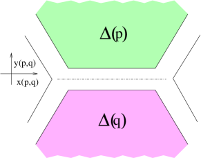
$\xrightarrow[y(p,q)\rightarrow 0]{\text{ADJACENCY LIMIT}}$  

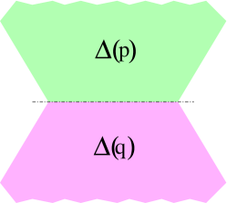
Figure 1: Shared boundaries in the adjacency limit.

Switching back to field theoretical contents, in this connection it is no longer correct to claim the presence of a vacuum state invariant under translations along the boundary: as a matter of fact, the shared boundary is obtained out of two separate loops, each of them being part of a domain where a BCFT is constructed, and all the associated Fock space elements are invariant under translation only along the relevant boundary loop.

Thus, in order for the geometric glueing process to be consistent with the functional data of the theory on each cylinder, we must require that the $N_{0}$ a priori independent Fock spaces blend pairwise without breaking the conformal and the chiral symmetry of the model.

Within this framework we can implement a non symmetry-breaking glueing of two adjacent cylindrical ends associating to such a pair a unique copy of the chiral algebras and of the Virasoro ones. Taking into account $z(q,p)=-z(p,q)$, we perform the glueing requiring a condition similar to (3) to hold. In this process, the subtle point resides in the maps $\Omega$ in (4). As a matter of fact, we must take into account that the whole process must relate the two glueing automorphisms $\Omega_{A(p)}$ and $\Omega_{B(q)}$ associated to the BCFTs defined respectively on $\Delta^{*}_{\varepsilon(p)}$ and $\Delta^{*}_{\varepsilon(q)}$. Thus it seems natural to introduce a further automorphism ${\Omega^{\prime}}^{A(p)B(q)}$ which, in the adjacency limit $y(p,q)=\Im\left[z(p,q)\right]\rightarrow 0$, acts along the boundary deforming continuously the (holomorphic and antiholomorphic components of the) bulk chiral fields in $\Delta^{*}_{\varepsilon(p)}$ into the corresponding counterpart on $\Delta^{*}_{\varepsilon(q)}$. To rephrase:

$$\mathbf{W}_{\Omega_{A(p)}}(z(p,q))|_{y(p,q)\rightarrow 0}={\Omega^{\prime}}^{A(p)B(q)}\mathbf{W}_{\Omega_{B(q)}}(z(p,q))|_{y(p,q)\rightarrow 0}.$$ (5)

In this way, we are indeed implementing a two way dynamical flow of informations between $\Delta^{*}_{\varepsilon(p)}$ and $\Delta^{*}_{\varepsilon(q)}$. As a matter of fact, (5) provides a concrete mean to associate to each pairwise adjacent set of conformal theories a unique chiral current out of (5):

$$\mathbb{W}_{{\Omega^{\prime}}_{A(p)B(q)}}\left(z(q,p)\right)=\begin{cases}\mathbf{W}_{\Omega_{A(p)}}\left(z(q,p)\right)&\text{in\;$\Delta^{*}_{\varepsilon(p)}$ $\cup\rho_{1}(p,q)$}\\ {\Omega^{\prime}}^{A(p)B(q)}\mathbf{W}_{\Omega_{B(q)}}\left(z(q,p)\right)&\text{in\;$\Delta^{*}_{\varepsilon(q)}$$\cup\rho_{1}(q,p)$}\end{cases}.$$ (6)

Expanding in Laurent series the field $\mathbb{W}_{{\Omega^{\prime}}_{A(p)B(q)}}\left(z(q,p)\right)$ in (6), we can associate a unique copy of the chiral algebra, namely $\mathcal{W}(p,q)$, to each pairwise adjacent pairs of BCFTs.

We have now introduced all the main ingredients we need in order to coherently define a full-fledged boundary conformal field theory on the whole surface $M_{\partial}$. As a matter of fact, we can associate to each $(p,q)$ pair of BCFTs defined on adjacent cylinders along a ribbon graph edge, a unique Hilbert space of states $\mathcal{H}^{(p,q)}$; the latter can be determined through the action of chiral modes of (6) on a true vacuum state, whose existence is granted per hypothesis. As usual, $\mathcal{H}^{(p,q)}$ gets decomposed into a direct sum of subspaces $\mathcal{H}_{\lambda(p,q)}$ which are carrier of an irreducible representation of the $\mathcal{W}(p,q)$ algebra itself. Exploiting the state-to-field correspondence, we can associate to each highest weight state in $\mathcal{H}_{\lambda(p,q)}$ a primary field which we shall refer to as Boundary Insertion Operators such that

$$\psi_{\lambda(q,p)}^{A(p)B(q)}(x(q,p))\,=\,\psi_{\lambda(p,q)}^{B(q)A(p)}(x(p,q)),$$ (7)

where $x(q,p)\,=\,\Re\left[z(q,p)\right]$. In (7) the notation is chosen with the following convention: $\lambda(p,q)$ is the representation label while the decoration with indexes $A(p)$ and $B(q)$ points out that the switch in boundary conditions actually refers to all parameters which specify the boundary assignment.

At this stage, BIOs are purely formal objects. However, their definition as conformal primaries allows to describe them as Chiral Vertex Operators, hence associating them a conformal dimension related to the highest weight of the associated Verma module. Nonetheless, in [16] we showed that the trivalent structure of the ribbon graph, on which BIOs are naturally defined, is sufficient to provide all the fundamental data defining their interaction. As a matter of fact, it allows to introduce their two point functions and OPEs as objects which are well defined respectively on ribbon graph’s edges and vertexes.

In the next session, we will find out in which particular cases we can characterize explicitly both their algebraic and analytic descriptions. Moreover, we will show that, once again, the structure of $\Gamma$ allows to fix the algebraic form of the OPEs’ coefficients.

3 Characterisation of Boundary Insertion Operators

To investigate BIOs properties, let us focus on the bulk theory identified by $D$ real embedding maps (scalar fields) $X^{\alpha}:\,M_{\partial}\rightarrow\mathcal{T}$, $\alpha=1,\ldots,D$, and let us introduce the following worldsheet action on the single $\Delta^{*}_{\varepsilon(p)}$:

$$S\,=\,\frac{1}{4\pi}\int d\zeta(p)d\bar{\zeta}(p)\,E_{\alpha\beta}(p)\left(\partial X^{\alpha}(p)\bar{\partial}\overline{X}^{\beta}(p)\right).$$ (8)

In (8), the background matrix $E(p)=G(p)+B(p)$ encodes target space information by specifying the background metric and Kalb-Ramond field components, respectively $G_{\alpha\beta}$ and $B_{\alpha\beta}$. In particular, let us deal with flat toroidal backgrounds, in which the $D$ directions are compactified and $E(p)$’s components are $X$-independent. The above configuration has an straightforward open-string interpretation: we are dealing with $N_{0}$ cylindrical ends whose outer boundary can, a priori, lay on a stack of $N$ $D$-branes. The latters, on one hand allow to decorate each open-string with a suitable assignment of $U(N)$ Chan-Paton factors (consequences of this from the glueing point of view are deeply analysed in [16]) while, on the other side, they act as sources of gauge fields, whose dynamic is encoded in the previous action (in the case of static brane and constraint field strength ) by means of the identification $F_{\alpha\beta}=\frac{1}{4\pi}B_{\alpha\beta}$. This obviously means that, if we consider a stack of $D-p$-branes, the Kalb-Ramond field is constrained to have non-zero components only along the first $p+1$ directions.

After the above premises, which ultimately show that the characterisation of the toroidal backgrounds we will deal with directly resides into the choice of a particular point into moduli space of inequivalent toroidal compactifications of $D$ directions, i.e. [17, 18]:

$$\mathcal{M}=O(D,D,\mathbb{Z})\backslash O(D,D)/[O(D)\times O(D)],$$

let us switch back to our main aim, namely the description of the algebraic structure and of the action of Boundary Insertion Operators. To this end, let us pick up those special orbits in moduli space which are fixed under the generalised $T$-duality group $O(D,D,\mathbb{Z})$. These moduli values give rise to theories in which the fundamental $[U(1)_{L}\times U(1)_{R}]^{D}$ current symmetry is enanched to different symmetry groups of rank at least $D$. In particular, if we break $U(N)\,\rightarrow U(1)^{N}$, in each abelian subsector we can choose the maximally enhanced symmetry background as [18]:

$$G_{\alpha\beta}=\frac{1}{2}C_{\alpha\beta}$$ (9a)

$$B_{\alpha\beta}=G_{\alpha\beta}\,\,\forall\,\alpha\,>\,\beta,\quad B_{\alpha\beta}=-\,G_{\alpha\beta}\,\,\forall\,\alpha\,<\,\beta,\quad B_{\alpha\alpha}=0,$$ (9b)

where if $C_{\alpha\beta},\,\alpha,\beta=1,\ldots,D$, is the Cartan matrix of a semisimple simply laced Lie algebra $\mathfrak{g}_{D}$ of total rank D.

When dealing with $p+1$ Neumann and $D-p-1$ Dirichlet directions, we are forced to set $B_{m,n}=0\,\forall m,n=p+1,\ldots D-p-1$, hence the maximally extended symmetry group will be:

$$\mathbb{G}_{D}\,=\,({G}_{p+1}\,\times{G}_{p+1})\,\times\,(SU(2)\times SU(2))^{D-p-1}.$$ (10)

Let us deal with a single factor ${G}_{r}\times G_{r}$ entering in (10), where ${G}_{r}$ is the universal covering group generated by the simply laced Lie algebra of rank $r$, $\mathfrak{g}_{r}$, whose Cartan matrix specifies the background matrix entries. The emerging of such an extended symmetry group is one hint of the quantum equivalence between such a theory of D free and compactified scalar bosons and the $\hat{\mathfrak{g}}_{k=1}$-WZW model, where $\hat{\mathfrak{g}}_{k=1}$ is the affine extension of $\mathfrak{g}_{r}$ at level $k=1$. Within this framework, the related bulk theory can be fully characterised by the properties of the WZW model. As a first remark, let us point out that the theory is rational, hence the infinite serie of Verma modules can be reorganised to write the Hilbert space of states as the direct sum of the finitely many irreps of the affine Lie algebra (now playing the role of the CFT chiral algebra):

$$\mathcal{H}^{(C)}\,=\,\bigoplus_{\hat{\omega}_{I}\in P_{+}^{1}(\hat{\mathfrak{g}})}\mathcal{H}_{\hat{\omega}_{I}}^{\hat{\mathfrak{g}}_{1}}\,\otimes\,\overline{\mathcal{H}}_{\hat{\omega}_{I}}^{\hat{\mathfrak{g}}_{1}}.$$ (11)

Denoting (the holomorphic part of) the primary fields associated to the highest weight state in $\mathcal{H}_{\hat{\omega}_{I}}^{\hat{\mathfrak{g}}_{1}}$ with $\phi_{\hat{I}(p)}(\zeta(p))$, we immediately notice that their components, $\phi_{[\hat{I}(p),\,m]}(\zeta(p))$, $m\,=\,1,\,\ldots,\,\text{dim}\hat{\omega}_{I}$, fill the level-0 (in sense of $L_{0}$ eigenvalue) subspace of $\mathcal{H}_{\hat{\omega}_{I}}^{\hat{\mathfrak{g}}_{1}}$, which we will denote with $\mathcal{V}_{\hat{\omega}_{I}}^{0}$. These last subspaces carry an irreducible representation of the horizontal subalgebra of $\hat{\mathfrak{g}}_{1}$:

$$\mathbf{X}^{\hat{I}}_{J_{0}}\,:\;\mathcal{V}_{\hat{\omega}_{I}}^{0}\,\rightarrow\,\mathcal{V}_{\hat{\omega}_{I}}^{0},$$ (12)

being $J_{0}$ generic element of $\mathfrak{g}$ [12].

To extend this RCFT on a surface with boundary, we can try to adopt Cardy’s construction: a set of boundary conditions that we can consistently define on the boundaries of a cylindrical domain are labelled exactly by the modules of the chiral algebra entering into the Hilbert space. The correspondent boundary states are [15]:

$$||\hat{\omega}_{I}(p)\rangle\negthinspace\rangle\,=\sum_{\hat{\omega}_{J}\,\in\,P_{+}^{1}(\hat{\mathfrak{g}})}\frac{\mathcal{S}_{\hat{I}\,\hat{J}}}{\sqrt{\mathcal{S}_{\hat{0}\,\hat{J}}}}|\hat{\omega}_{J}(p)\rangle\negthinspace\rangle.$$ (13)

However, as they stand, Cardy’s boundary states are necessary but not sufficient to describe the boundary extension of our CFT. To fully classify the plethora of boundary assignments we can coherently fix for our model, we have to call into play the concept of BCFT deformation.

Let us remember that, given a BCFT with bulk action $S_{bulk}$, fluctuations in the boundary condensate can move the theory away from the Renormalisation Group fixed point, defining a new theory with action $S=S_{bulk}+g\int{dx\psi(x)}$. If the perturbing field $\psi(x)$ is a truly marginal boundary field, the boundary term in the action does not break the conformal invariance; hence, the set of coefficients $\{g\}$ entering in previous formula parametrises a set of BCFTs differing from the unperturbed one only for a redefinition of boundary conditions and of the related boundary states.

This is exactly what happens in our case: as a matter of fact, let us remember that, at fixed points in toroidal compactifications moduli space, both the set of bulk chiral currents and the set of open string scalar states get enlarged. If we define the new holomorphic and antiholomorphic bulk chiral currents with $J^{a}(\zeta)$ and $\overline{J}^{a}(\bar{\zeta})$, we can represent vertex operators associated the new open string scalars as $S^{a}_{\lambda}(u)e^{i\lambda_{i}X^{i}(u)}\doteq\left.\frac{1}{2}\left[J^{a}(\zeta)+\overline{J}^{a}(\bar{\zeta})\right]e^{i\lambda_{i}X^{i}(\zeta)}\right|_{|\zeta|=1|\zeta|=e^{\frac{2\pi}{2\pi-\varepsilon(p)}}}$. Hence, the associated currents can be combined to deform the theory. The most general perturbing term will be [19, 20]:

$$S_{B}\,=\,\int du\sum_{a}g_{a}\mathbf{J}^{a}(\zeta)|_{|\zeta|=1}=\int du\left(\sum_{\hat{\alpha}}g_{\hat{\alpha}}\,e^{i\hat{\alpha}_{i}\,X^{i}}+\sum_{i}g_{i}\partial_{x}X^{i}\right)|_{|\zeta(p)|=1}.$$ (14)

However, chiral marginal deformations are truly marginal ones: hence, the deformed model will change only for a redefinition of boundary conditions (hence boundary states and boundary field spectra). In this connection, the full set of boundary states can be represented as the following rotation of the one associated to the unperturbed theory [19, 20]:

$$\|g\rangle\negthinspace\rangle\,=\,e^{i\sum\limits_{\hat{\alpha}}g_{\hat{\alpha}}E_{0}^{\hat{\alpha}}\,+\,i\sum\limits_{i}g_{i}H^{i}_{0}}\|B\rangle\negthinspace\rangle_{free}.$$ (15)

where the rotation group element acting on $\|B\rangle\negthinspace\rangle_{free}$ is uniquely determined by the boundary action (14).

After this rather length but necessary premise, we can came back to our purpose, trying to describe Boundary Insertion Operators in this background. The above characterization of boundary states is instrumental but not completely useful to this aim. To overcome this problem, we showed that, among the boundary states in (15), we can identify Cardy’s ones as those generated by a rotation induced by an element in the centre of the universal covering group $G_{r}$:

$$\|\hat{\omega}_{I}\rangle\negthinspace\rangle=b_{A_{I}}\|\hat{\omega}_{0}\rangle\negthinspace\rangle,$$ (16)

where $b_{A_{I}}=e^{-2\pi iA_{I}\hat{\omega}_{0}\cdot H}\in B(G_{r})$ is the central element uniquely associated to algebra outer automorphism $A_{I}$ which generates the fundamental weight $\hat{\omega}_{I}$ out of the basic one $\hat{\omega}_{0}$.

Thanks to (16), we introduced an alternative parametrisation of the above set of boundary conditions as the doublet

$$\left[\|\hat{\omega}_{I}\rangle\negthinspace\rangle,\,\Gamma(k)\right],\qquad\text{with}\quad\begin{cases}\hat{\omega}_{I}&\,\in\,P_{+}^{1}(\hat{\mathfrak{g}})\\ \Gamma(k)&\,\in\,\frac{G_{r}}{B(G_{r})}\end{cases}$$ (17)

being $\|\hat{\omega}_{I}\rangle\negthinspace\rangle$ a Cardy’s boundary state and $\Gamma(k)\in\frac{G_{r}}{B(G_{r})}$ such that:

$$\|g(k)\rangle\negthinspace\rangle\,=\,\Gamma(k)\,\|\hat{\omega}_{J}(k)\rangle\negthinspace\rangle.$$ (18)

Moreover, we showed that the above parametrisation is not only a formal datum, but it allows to re-describe the model as a deformation of the $\hat{\mathfrak{g}}_{k=1}$-WZW model described “á la Cardy” by means of the boundary term $S_{\Gamma}=\int du\Gamma_{a}J^{a}(u)$ such that we can define its coefficients through a suitable immersion of $\Gamma(k)$ into the universal covering group $G_{r}$:

$$\sigma:\;\Gamma\in\frac{G_{r}}{B(G_{r})}\hookrightarrow e^{i\Gamma_{a}J^{a}_{0}}\in G_{r}$$ (19)

This description allowed firstly to characterize completely the glueing automorphism $\Omega_{[\hat{J}_{2},\Gamma_{2}](q)\,[\hat{J}_{1},\Gamma_{1}](p)}$ entering in (6) by means of:

• the fusion coefficients $\mathcal{N}_{\hat{J}(p)\,\hat{I}(p,q)}^{\hat{J}(q)}$ of the WZW model,

• a deformation induced by the rotation $\Gamma(p,q)=\Gamma_{2}(q)\Gamma_{1}(p)^{-1}$.

Moreover, we gathered the following expression for Boundary Insertion Operators’ components in the rational limit of the conformal theory:

$$\psi^{[\hat{J}_{2},\,\Gamma_{2}](q)\,[\hat{J}_{1},\,\Gamma_{1}](p)}_{[\hat{I},\,m](p,q)}\,=\,\sum_{n=0}^{\text{dim}|\hat{I}|}R^{\hat{I}(p,q)}_{m\,n(p,q)}(\Gamma_{2}{\Gamma_{1}}^{-1})\,\psi_{[\hat{I},\,n](p,q)}^{\hat{J}_{2}(q)\,\hat{J}_{1}(p)},$$ (20)

where $\psi_{\hat{J}(p,q)}^{\hat{J}(p)\,\hat{J}(q)}(x(p,q))\,=\,\mathcal{N}_{\hat{J}(p)\,\hat{I}(p,q)}^{\hat{J}(q)}\,\psi_{\hat{I}(p,q)}(x(p,q))$ and where $R^{\hat{I}(p,q)}_{m\,n(p,q)}=\exp\left[\frac{i}{2}X^{\hat{I}(p,q)}\right]_{m\,n(p,q)}$ being $X^{\hat{I}}$ the operator introduced in (12).

4 Discussions and conclusions

Boundary Insertion Operators, defined as in equation (20), have a beautiful feature: the boundary perturbation induced by $\Gamma(p,q)$ does not affect their algebra, which hence is completely fixed in terms of the fusion rules of the WZW-model. This is indeed a check that our prescription for the $(p,q)$ glueing automorphism and its subsequent action on BIOs is consistent. As a matter of fact all deformations we have introduced are actually truly marginal ones and, thus, they must not break the chiral symmetry defined by $\hat{\mathfrak{g}}$. Hence, the expansion coefficients of the product between $\psi^{[\hat{J}_{1},\,\Gamma_{1}](p)\,[\hat{J}_{3},\,\Gamma_{3}](r)}_{\hat{I}_{1}(r,p)}(\omega_{r})$ and $\psi^{[\hat{J}_{3},\,\Gamma_{3}](r)\,[\hat{J}_{2},\,\Gamma_{2}](q)}_{\hat{I}_{2}(q,r)}(\omega_{q})$ in terms of $\psi^{[\hat{J}_{1},\,\Gamma_{1}](p)\,[\hat{J}_{2},\,\Gamma_{2}](q)}_{\hat{I}_{3}(q,p)}(\omega_{p})$ can be written uniquely as $\mathcal{C}_{\hat{I}_{1}(r,p)\,\hat{I}_{2}(q,r)\,\hat{I}_{3}(q,p)}^{\hat{J}_{1}(p)\,\hat{J}_{3}(r)\,\hat{J}_{2}(q)}$.

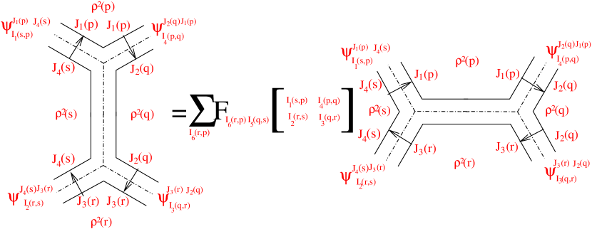
Figure 2: Four-points function crossing symmetry.

The final piece of the puzzle we are trying to make up comes directly from the study of the four-point function among BIOs. This is naturally defined in the neighbourhood of four adjacent cylindrical ends, hence its computation calls into play the variable connectivity of random Regge triangulations, which produces the same feature on the ribbon graph. Hence, if we notice that the two factorisations through which we can compute the four-point function are strictly related to the two ways we can fix the connectivity among the surrounding polytopes (see figure 2), we can write an identity formally equivalent to the usual Pentagonal Identity for BCFT [21, 22, 23]. This allows to identify BIO’s OPE coefficients describing interactions in the neighbourhood of the $(p,q,s)$ vertex of the ribbon graph with the $\hat{\mathfrak{g}}$-WZW model fusion matrices with the following entries assignments[24]:

$$\mathcal{C}^{\hat{J}_{1}(p)\,\hat{J}_{2}(q)\,\hat{J}_{3}(s)}_{\hat{I}_{1}(q,p)\,\hat{I}_{2}(s,q)\,\hat{I}_{3}(s,p)}\,=\,F_{\hat{J}_{2}(q)\,\hat{I}_{3}(s,p)}\begin{bmatrix}\hat{J}_{1}(p)&\hat{J}_{3}(s)\\ \hat{I}_{1}(q,p)&\hat{I}_{2}(s,q)\end{bmatrix}.$$ (21)

This naturally completes the programme we outlined at the beginning of this paper. The algorithm we presented has a twofold value. From one hand, we have been able to provide an explicit expression for the formal rules describing the interplay among BCFTs on different cylinders whenever we consider toroidal compactifications for the target space of the bosonic scalar field. On the other side, the open string interpretation we gave at the beginning of section 3 provides a natural way to colour the ribbon graph (defined as the edge refinement of the 1-skeleton barycentrically dual to a random Regge triangulation), with labels proper of the chosen gauge group. This ultimately leads to the constructions of a genuine ’t Hooft diagram and to the definition of new kinematical background in which we investigate dynamical processes which are characteristic in open/closed string dualities.

References

- [1] R. Dijkgraaf and C. Vafa, Nucl. Phys. B 644 (2002) 3 [arXiv:hep-th/0206255].
- [2] D. Gaiotto and L. Rastelli, JHEP 0507, 053 (2005) [arXiv:hep-th/0312196].
- [3] R. Gopakumar, Phys. Rev. D 70, 025009 (2004) [arXiv:hep-th/0308184].
- [4] R. Gopakumar, Phys. Rev. D 70, 025010 (2004) [arXiv:hep-th/0402063].
- [5] R. Gopakumar, Comptes Rendus Physique 5, 1111 (2004) [arXiv:hep-th/0409233].
- [6] R. Gopakumar, Phys. Rev. D 72, 066008 (2005) [arXiv:hep-th/0504229].
- [7] O. Aharony, Z. Komargodski and S. S. Razamat, JHEP 0605, 016 (2006) [arXiv:hep-th/0602226].
- [8] J. R. David and R. Gopakumar, arXiv:hep-th/0606078.
- [9] M. Mulase and M. Penkava arXiv:math-ph/9811024.
- [10] M. Carfora and A. Marzuoli, Adv. Theor. Math. Phys. 6 (2003) 357 [arXiv:math-ph/0107028].
- [11] M. Carfora, C. Dappiaggi and A. Marzuoli, Class. Quant. Grav. 19 (2002) 5195 [arXiv:gr-qc/0206077].
- [12] A. Recknagel and V. Schomerus, Nucl. Phys. B 545, 233 (1999) [arXiv:hep-th/9811237].
- [13] M. R. Gaberdiel, Fortsch. Phys. 50, 783 (2002).
- [14] P. Di Francesco, P. Matheu, and D. Sénéchal. Conformal Field Theory. Springer-Verlag, New York Inc., 1996.
- [15] John L. Cardy. Nucl. Phys., B324:581, 1989.
- [16] Valeria L. Gili. PhD thesis, Università degli Studi di Pavia, 2006. hep-th/0605053.
- [17] Clifford v. Johnson. D-branes. Cambridge Monographs on Mathematical Physics, 2003.
- [18] Amit Giveon, Massimo Porrati, and Eliezer Rabinovici. Phys. Rept., 244:77–202, 1994. hep-th/9401139.
- [19] Ali Yegulalp. Nucl. Phys., B450:641–662, 1995. hep-th/9504104.
- [20] Michael B. Green and Michael Gutperle. Nucl. Phys., B460:77–108, 1996. hep-th/9509171.
- [21] Ingo Runkel. Nucl. Phys., B549:563–578, 1999. hep-th/9811178.
- [22] Roger E. Behrend, Paul A. Pearce, Valentina B. Petkova, and Jean-Bernard Zuber. Nucl. Phys., B570:525–589, 2000. hep-th/9908036.
- [23] Giovanni Felder, Jurg Frohlich, Jurgen Fuchs, and Christoph Schweigert. J. Geom. Phys., 34:162–190, 2000. hep-th/9909030.
- [24] Luis Alvarez-Gaume, C. Gomez, and G. Sierra. Phys. Lett., B220:142, 1989.