1 Introduction

Three quarters of a century have passed since the introduction of magnetic monopoles in quantum field theory by Dirac [1]. Our understanding of the soliton sector of spontaneously broken gauge theories [2] is still largely unsatisfactory. In particular, the development in our understanding of non-Abelian versions of monopoles [3]-[17] and vortices [18] have been very slow, in spite of many articles written on these subjects, and in spite of the important role these topological excitations are likely to play in various areas of physics. For instance, they might hold the key to the mystery of quark confinement in Quantum Chromodynamics (QCD). Their quantum mechanical properties are gradually emerging, however, thanks to an ever improving grasp on the nonperturbative dynamics in the context of supersymmetric gauge theories. Some of the ingredients of this development include the Seiberg-Witten solution of ${\cal N}=2$ supersymmetric gauge theories and exact instanton summations, better understanding of the properties of (super-) conformal field theories, exact results on the chiral condensates and symmetry breaking pattern in a wide class of ${\cal N}=1$ supersymmetric gauge theories, and so on. Also, many new results on non-Abelian vortices and domain walls are now available, which are closely related to the problems concerning the monopoles.

It is the author’s opinion that a serious discussion about confinement and non-Abelian monopoles today cannot ignore these basic results from supersymmetric gauge theories. This lecture presents a review of what the author believes to be some of the most relevant aspects of this development, which should serve as an introduction to this very exciting area of research.

2 Color confinement

One of the profound unsolved problems in the elementary particle physics today is quark confinement. A popular idea, due to ’t Hooft and Mandelstam [19] holds that the ground state of QCD (quantum chromodynamics) is a dual superconductor: the quarks are confined by the chromo-electric vortices, analogous to the magnetic Abrikosov-Nielsen-Olesen vortex in the usual type II superconductors in solid. The Lagrangian of QCD

$$L=-\frac{1}{4}F_{\mu\nu}^{a}F^{\mu\nu\,a}+{\bar{\psi}}\,(i\gamma_{\mu}\,{\cal D}^{\mu}+m)\,\psi$$ (1)

however describes the dynamics of quarks and gluons, and it is not obvious from (1) how magnetic (dual) degrees of freedom appear and how they interact. One way to detect such degrees of freedom is ’t Hooft’s Abelian gauge fixing. One chooses the gauge so that a given field (perhaps some composite of $F_{\mu\nu}^{a}$) in the adjoint representation to take an Abelian form

$$X=\left(\begin{array}[]{ccc}\lambda_{1}&0&0\\ 0&\lambda_{2}&0\\ 0&0&\lambda_{3}\end{array}\right),\qquad\lambda_{1}>\lambda_{2}>\lambda_{3}.$$ (2)

For a generic gauge-field configuration $A_{\mu}(x)$, however, it is not possible to keep the above diagonal form everywhere in ${\bf R}^{4}$. Near a singularity $\lambda_{1}=\lambda_{2}$, diagonalization of the matrix

$$X=X|_{\lambda_{1}=\lambda_{2}}+\left(\begin{array}[]{cc}C(x)&0\\ 0&0\end{array}\right)$$ (3)

where $C$ is a $2\times 2$ matrix, for instance, of the form,

$$C=\tau^{i}(x-x_{0})^{i},$$ (4)

by a gauge transformation $U(x)$, introduces a magnetic monopole, $A_{i}\simeq U(x)\,\partial\,U(x)^{-1}$.

Another possibility is to use the Cho-Faddeev-Niemi decomposition [20] of the gauge fields (for $SU(2)$)

$$A_{\mu}^{a}=C_{\mu}{\bf n}^{a}+{\tilde{\sigma}}(x)(\partial_{\mu}{\bf n}\times{\bf n})^{a}+\rho\,\partial_{\mu}{\bf n}^{a};\qquad{\tilde{\sigma}}(x)=1+\sigma(x),$$ (5)

in terms of the unit vector field ${\bf n}$ and the Abelian gauge field $C_{\mu}$ which live on $S^{2}$ and $S^{1}$ factors, respectively, of $SU(2)$, and a charged ”scalar” field

$$\phi=\rho(x)+i\sigma(x).$$ (6)

The Wu-Yang singular monopole solution [21], for instance, corresponds to

$$n^{a}=\frac{x^{a}}{r},\quad C_{\mu}=\phi=0.$$ (7)

It is possible that these singularities, regularized e.g., by the zero of $1-|\phi|^{2}$, somehow manage to behave as dominant degrees of freedom in the ground state of QCD.

Whichever way, a central question is whether the magnetic monopoles of QCD is of Abelian or non-Abelian type. The ’t Hooft-Mandelstam scenario is essentially Abelian. By assuming that the relevant infrared degrees of freedom are those which signal the singularities of Abelian gauge fixing, one tacitly makes a highly nontrivial dynamical assumption.

In this respect, the $SU(2)$ gauge theory is an exception, though. It is quite possible that in this particular case ’t Hooft’s (or related) Abelian gauge fixing procedure allows us to “detect” the correct magnetic degrees of freedom, even if the system does not dynamically Abelianize . The singularities of the Abelian gauge-fixing would signal the presence of the magnetic degrees of freedom, which correspond [22] just to the Wu-Yang monopoles, Eq. (7). As the Cho-Faddeev-Niemi $n_{a}(x)$ field parametrizes $\pi_{2}(S^{2})\sim\pi_{2}(SU(2)/U(1))={\bf Z}$, the magnetic charge of the Wu-Yang monopoles are the same, and quantized in the same way, as the ’t Hooft-Polyakov monopoles of the Georgi-Glashow model. In more general $SU(N)$ theories with $N\geq 3$, however, one does not expect such a lucky situation. If the system does not dynamically Abelianize to $U(1)^{N-1}$ effective system at some low-energy scales, it would not be appropriately described by an effective Lagrangian describing the Abelian monopoles which signal the singularities of the Abelian gauge fixing.

Actually, there is no hint that such a dynamical scenario (dynamical Abelianization) is realized in Nature. We must seriously consider the much more subtle possibility that somehow non-Abelian, magnetic degrees of freedom play a role in the physics of confinement and chiral symmetry breaking. Are there models in which the low-energy dynamics is known and in which non-Abelian magnetic degrees of freedom play a central role?

It does not seem to be widely known that not only do such systems exist, but that in a sense this (occurrence of light non-Abelian monopoles) is a most typical dynamical phenomenon in a wide class of supersymmetric gauge systems. The class of models in question is $N=2$ supersymmetric theories with $SU$, $SO$ or $USp$ gauge groups with quark hypermultiplets in various representations [23]-[31]. Moreover, the class of models in which one can make reliable analysis about their low-energy behavior, have increased enormously thanks to a more recent work on certain $N=1$ models [32] with scalar multiplets in the adjoint representation. Again, the appearance of massless, non-Abelian monopoles in their low-energy effective action is a rule, rather than an exception, in these models.

Of course, in the context of superconformal theories there are famous examples of non-Abelian dualities such as the Montonen-Olive duality in $N=4$ supersymmetric theories [33] or the Seiberg duality in the $N=1$ supersymmetric models [34] with nontrivial infrared fixed points.

These problems (conformal invariance and confinement) are closely related, as the confinement and dynamical symmetry breaking can often be seen as the result of breaking of (nontrivial) conformal invariance near an infrared-fixed point theory.

Evidently, supersymmetric theories are trying to tell us something important about the non-Abelian monopoles and confinement. In what follows we review briefly the old difficulties associated with the semiclassical concepts of non-Abelian monopoles. It will be argued that the dual group properties of non-Abelian monopoles occurring in a system with gauge symmetry breaking $G\,\,\,\longrightarrow\,\,\,H$ are best defined by setting the low-energy $H$ system in Higgs phase, so that the dual system is in confinement phase. The transformation law of the monopoles follows from that of monopole-vortex mixed configurations in the system with a large hierarchy of energy scales, $v_{1}\gg v_{2}$,

$$G\,\,\,{\stackrel{{\scriptstyle v_{1}}}{{\longrightarrow}}}\,\,\,H\,\,\,{\stackrel{{\scriptstyle v_{2}}}{{\longrightarrow}}}\,\,\,{\bf 1},$$ (8)

under an unbroken, exact color-flavor diagonal symmetry $H_{C+F}$ This last symmetry is broken by individual soliton vortex, so the latter develops continuous moduli. The transformation law among the regular monopoles, which appear at the endpoint of the vortex, follows from that of the vortices. This defines, once rewritten in the dual, magnetic variables, the dual group ${\tilde{H}}$ under which the monopoles transform as a multiplet.

3 Semiclassical “non-Abelian monopoles”: difficulties

3.1 Abelian monopoles

A system in which the gauge symmetry is spontaneously broken

$$G\,\,\,{\stackrel{{\scriptstyle\langle\phi_{1}\rangle\neq 0}}{{\longrightarrow}}}\,\,\,H$$ (9)

where $H$ is some non-Abelian subgroup of $G$, possesses a set of regular magnetic monopole solutions in the semi-classical approximation. They are natural generalizations of the Abelian ’t Hooft-Polyakov monopoles [2], found originally in the $G=SO(3)$ theory broken to $H=U(1)$ by a Higgs mechanism. In that theory, the field content is just the $SU(2)$ gauge fields and a scalar field in the adjoint representation of the gauge group; the energy of a static field configuration has an expression

$$E=\int d^{3}x[\,\frac{1}{4}F_{ij}^{a\,2}+\frac{1}{2}(D_{i}\phi^{a})^{2}+\frac{\lambda}{8}(\phi^{a\,2}-F^{2})^{2}\,]$$ (10)

where

$$F_{ij}^{a}=\partial_{i}\,A_{j}-\partial_{j}\,A_{i}-g\,\epsilon^{abc}\,A_{i}^{b}\,A_{j}^{c};$$

while $D_{i}\phi^{a}$ is a covariant derivative,

$$D_{i}\phi^{a}=\partial_{i}\phi^{a}-g\,\epsilon^{abc}A_{i}^{b}\,\phi^{c}.$$

Now the static finite energy solution of the equation of motion must behave asymptotically as

$$\phi^{a}\to n^{a}(x)\,F,\qquad n^{a}(x)^{2}=1,$$ (11)

where the vector field $n^{a}(x)$ clearly label the winding of the map $S^{2}\to S^{2}$, the first sphere being the space sphere surrounding the monopole, the second sphere representing the vacuum orientation in the group space. One possibility is $n^{a}$ has a fixed orientation, such as $n^{a}(x)=(0,0,1)$ everywhere: this represents a vacuum. Another possibility is that $n^{a}$ makes a nontrivial winding in the group space as $x_{i}$ goes around the sphere, e.g.

$$n^{a}(x)=(\sin\theta\,\cos m\phi,\sin\theta\,\sin m\phi,\cos\theta),\qquad m=\pm 1,\pm 2,\ldots.$$

This integer labels the homotopy classes

$$\pi_{2}(SU(2)/U(1))\sim\pi_{2}(S^{2})\sim{\mathbf{Z}}$$

of the scalar field configurations. The gauge fields must reduce to the pure gauge,

$$A_{i}^{a}\to\frac{1}{g}\epsilon^{abc}\,n^{b}(x)\,\partial_{i}\,n^{c}(x)$$

in order for the energy to be finite.

The solution of the equation of motion in the nontrivial sectors can be found by rewriting Eq. (10) as

$$E=\int d^{3}x[\,\frac{1}{4}(F_{ij}^{a}-\epsilon_{ijk}\,D_{k}\phi^{a})^{2}+\frac{1}{2}\epsilon_{ijk}\,F_{ij}^{a}\,D_{k}\,\phi^{a}+\frac{\lambda}{8}(\phi^{a\,2}-F^{2})^{2}$$ (12)

The crucial observation is that while the first and third terms are semi-positive definite, the second term is a total derivative,

$$\frac{1}{2}\epsilon_{ijk}\,F_{ij}^{a}\,D_{k}\,\phi^{a}=\partial_{k}\,B_{k},\qquad B_{k}=\frac{1}{2}\epsilon_{ijk}\,F_{ij}^{a}\,\phi^{a}.$$

We used above a useful identity for the derivatives for gauge invariant products

$$\partial_{k}\,{\rm Tr}(A\,B\,\ldots)={\rm Tr}(D_{k}A\,B\,\ldots)+{\rm Tr}(A\,D_{k}B\,\ldots)+\ldots.$$

Thus the second term of Eq. (12) represents $F$ times the “magnetic” charge

$$\int dv\,\nabla\cdot{\bf B}=\int dS\cdot{\bf B}=4\,\pi g_{m},\qquad{\bf B}\sim\frac{g_{m}}{r^{3}}\,{\bf r}.$$

If $\lambda=0,$ $|\phi^{a\,2}|\to F^{2}$ (BPS limit) the mass is proportional to the magnetic charge, $4\,\pi\,g_{m}\,F=\frac{\langle\phi\rangle}{g}$, while the field configuration satisfies the linear BPS equation

$$F_{ij}^{a}-\epsilon_{ijk}\,D_{k}\phi^{a}=0,$$

with an explicit (BPS) solution [2]

$$A_{i}^{a}=\epsilon_{aij}r_{j}\frac{1-K(r)}{g\,r^{2}},\qquad K(r)=\frac{gFr}{\sinh gFr},$$ (13)

$$\phi^{a}=r^{a}\,\frac{H(r)}{g\,r^{2}},\qquad H(r)=gFr\coth gFr-1.$$ (14)

3.2 Non-Abelian unbroken group

When the “unbroken” gauge group is non-Abelian, the asymptotic gauge field can be written as

$$F_{ij}=\epsilon_{ijk}B_{k}=\epsilon_{ijk}\frac{r_{k}}{r^{3}}({\beta}\cdot{\bf H}),$$ (15)

in an appropriate gauge, where ${\bf H}$ are the diagonal generators of $H$ in the Cartan subalgebra. A straightforward generalization of the Dirac’s quantization condition leads to

$$2\,{\beta\cdot\alpha}\in{\bf Z}$$ (16)

where $\alpha$ are the root vectors of $H$.

The constant vectors $\beta$ (with the number of components equal to the rank of the group $H$) label possible monopoles. It is easy to see that the solution of Eq. (16) is that $\beta$ is any of the weight vectors of a group whose nonzero roots are given by

$$\alpha^{*}=\frac{\alpha}{\alpha\cdot\alpha}.$$ (17)

This is just a standard group theory theorem: Eq. (16) can in fact be rewritten as the well-known relation between a weight vector and a root vector of any group, $2\,{\beta\cdot\alpha^{*}}/(\alpha^{*}\cdot\alpha^{*})\in{\bf Z}$.

The group generated by Eq. (17) is known as the dual (we shall call it GNOW dual below) of $H$, let us call ${\tilde{H}}$. One is thus led to a set of semi-classical degenerate monopoles, with multiplicity equal to that of a representation of ${\tilde{H}}$; this has led to the so-called GNOW conjecture, ı.e., that they form a multiplet of the group ${\tilde{H}}$, dual of $H$ [4]-[6]. For simply-laced groups (with the same length of all nonzero roots) such as $SU(N)$, $SO(2N)$, the dual of $H$ is basically the same group, except that the allowed representations tell us that

$$U(N)\leftrightarrow U(N);\qquad SO(2N)\leftrightarrow SO(2N),$$ (18)

while

$$SU(N)\leftrightarrow\frac{SU(N)}{{\mathbf{Z}}_{N}};\qquad SO(2N+1)\leftrightarrow USp(2N).$$ (19)

There is no difficulty in explicitly constructing these degenerate set of monopoles [6]. The basic idea is to embed the ’t Hooft-Polyakov monopoles in various broken $SU(2)$ subgroups. The main results are summarized in Appendix A, Appendix B. These set of monopoles constitute the prime candidates for the members of a multiplet of the dual group ${\tilde{H}}$.

There are however well-known difficulties with such an interpretation. The first concerns the topological obstruction discussed in [11]-[16]: in the presence of the classical monopole background, it is not possible to define a globally well-defined set of generators isomorphic to $H$. As a consequence, no “colored dyons” exist. In a simplest case with the breaking

$$SU(3)\,\,\,{\stackrel{{\scriptstyle\langle\phi_{1}\rangle\neq 0}}{{\longrightarrow}}}\,\,\,SU(2)\times U(1),$$ (20)

this means that

$${no\,\,monopoles\,\,with\,\,charges}\quad({\underline{2}},1^{*})\quad{exist},$$ (21)

where the asterisk indicates a dual, magnetic charge.

The second can be regarded as an infinitesimal version of the same difficulty: certain bosonic zero modes around the monopole solution, corresponding to $H$ gauge transformations, are non-normalizable (behaving as $r^{-1/2}$ asymptotically). Thus the standard procedure of quantization leading to $H$ multiplets of monopoles, does not work. Some progress on the check of GNOW duality along this orthodox line of thought, has been reported nevertheless [14], in the context of ${\cal N}=4$ supersymmetric gauge theories. Their approach, however, requires the consideration of particular class of multi monopole systems, neutral with respect to the non-Abelian group (more precisely, non-Abelian part of) $H$ only.

Both of these difficulties concern the transformation properties of the monopoles under the subgroup $H$, while the relevant question should be how they transform under the dual group, ${\tilde{H}}$. As field transformation groups, $H$ and ${\tilde{H}}$ are relatively nonlocal, the latter should look like a nonlocal transformation group in the original, electric description.

Another related question concerns the multiplicity of the monopoles: Take again the case of the system with a breaking pattern, Eq. (20). One might argue that there is only one monopole, as all the degenerate solutions are related by the unbroken gauge group $H=SU(2)$. Or one might say that there are two monopoles, in the sense that according to the semiclassical GNO classification they are supposed to belong to a doublet of the dual $SU(2)$ group. Or, perhaps, one should conclude that there are infinitely many, continuously related solutions, as the two solutions obtained by embedding the ’t Hooft solutions in $(1,3)$ and $(2,3)$ subspaces, are clearly part of the continuous set of (moduli of) solutions. In short, what is the multiplicity (${\cal N}$) of the monopoles:

$${\cal N}=1,\quad 2,\quad{\rm or}\quad\infty\,\,?$$ (22)

Formulated perhaps more adequately:

What is the dual group?

How do the degenerate magnetic monopoles transform among themselves under the dual group?

Which of the semiclassical aspects of monopoles survive quantum effects?

In the attempt to answer these questions, some general considerations seem to be unavoidable. The first is the fact since $H$ and $\tilde{H}$ groups are non-Abelian the dynamics of the system should enter the problem in essential way. For instance, the non-Abelian $H$ interactions can become strongly-coupled at low energies and can break itself dynamically. This indeed occurs in pure ${\cal N}=2$ super Yang-Mills theories (i.e., theories without quark hypermultiplets), where the exact quantum mechanical result is known in terms of the Seiberg-Witten curves [23]-[25]: see below. Consider for instance, a pure ${\cal N}=2$, $SU(N+1)$ gauge theory. Even though partial breaking, e.g., $SU(N+1)\to SU(N)\times U(1)$ looks perfectly possible semi-classically, in an appropriate region of classical degenerate vacua, no such vacua exist quantum mechanically. In all vacua the light monopoles are abelian, the effective, magnetic gauge group being $U(1)^{N}$.

Generally speaking, the concept of a dual group multiplet is well-defined when ${\tilde{H}}$ interactions are weak (or at worst, conformal). This however means that one must study the original, electric theory in the regime of strong coupling, which would usually make the task exceedingly difficult. Fortunately, in ${\cal N}=2$ supersymmetric gauge theories, exact Seiberg-Witten curves describe the fully quantum mechanical consequences of the strong-interaction dynamics in terms of weakly-coupled dual magnetic variables. This is how we know that the non-Abelian monopoles exist in fully quantum theories [27]: in the so-called $r$-vacua of softly broken ${\cal N}=2$, $SU(N)$ gauge theory, the light monopoles appear as the dominant infrared degrees of freedom and interact as pointlike particles having the charges of a fundamental multiplet ${\underline{r}}$ of an effective, dual $SU(r)$ gauge group. In an $SU(3)$ gauge theory broken to $SU(2)\times U(1)$ as in (20), with an appropriate number of quark multiplets ($N_{f}\geq 4$), for instance, light magnetic monopoles carrying the charges

$$({\underline{2^{*}}},1^{*})$$ (23)

under the dual $SU(2)\times U(1)$ appear in the low-energy effective action. (Dual) colored dyons do exist! The distinction between $H$ and ${\tilde{H}}$ is crucial (cfr. Eq. (21)).

In ${\cal N}=2$, $SU(N)$ SQCD with $N_{f}$ flavors, light non-Abelian monopoles with $SU(r)$ dual gauge group appear for $r\leq\frac{N_{f}}{2}$ only. Such a limit clearly reflects the dynamics of the soliton monopoles under renormalization group: the effective low-energy gauge group must be either infrared free or conformally invariant, in order for the monopoles to emerge as recognizable low-energy degrees of freedom [28]-[30].

A closely related point concerns the phase of the system. If the dual group were in Higgs phase, the multiplet structure among the monopoles would get lost, generally. Therefore one must study the dual (${\tilde{H}}$) system in confinement phase. But then, according to the standard electromagnetic duality argument, one must analyze the electric system in Higgs phase. The monopoles will appear confined by the vortices of the $H$ system, which can be naturally interpreted as confining string of the dual system ${\tilde{H}}$.

We are thus led to study the system with a hierarchical symmetry breaking,

$$G\,\,\,{\stackrel{{\scriptstyle v_{1}}}{{\longrightarrow}}}\,\,\,H\,\,\,{\stackrel{{\scriptstyle v_{2}}}{{\longrightarrow}}}\,\,\,{\bf 1},$$ (24)

where

$$v_{1}\gg v_{2},$$ (25)

instead of the original system (9). The smaller VEV breaks $H$ completely. However, in order for the degeneracy among the monopoles not to be broken by the breaking at the scale $v_{2}$, we require that some global color-flavor diagonal group

$$H_{C+F}\subset H_{color}\otimes G_{F}$$ (26)

remains unbroken (see below).

As we shall see, such a scenario is very naturally realized in ${\cal N}=2$ supersymmetric theories. An important lesson one learns from these considerations (and from the explicit models), is that the role of the massless flavor is fundamental. This manifests itself in more than one ways.

(i)

$H$ must be non-asymptotically free, this requires that there be sufficient number of massless flavors: otherwise, $H$ interactions would become strong at low energies and $H$ group can break itself dynamically;

(ii)

The physics of the $r$ vacua [28, 30] indeed shows that the non-Abelian dual group $SU(r)$ appear only for $r\leq\frac{N_{f}}{2}$. This limit can be understood from the renormalization group: in order for a nontrivial $r$ vacuum to exist, there must be at least $2\,r$ massless matter flavor in the original, electric theory;

(iii)

Non-abelian vortices [35, 37], which as we shall see are closely related to the concept of non-Abelian monopoles, require also an exact flavor group. The non-Abelian flux moduli arise as a result of an exact color-flavor diagonal symmetry of the system, broken by individual soliton vortices.

4 Non-Abelian monopoles from vortex moduli

It turns out that the properties of the monopoles induced by the breaking

$$G\to H$$ (27)

are closely related to the properties of the vortices, which develop when the low-energy $H$ gauge theory is put in Higgs phase by a set of scalar VEVs, $H\to{\bf 1}$. The crucial instrument is the exact homotopy sequence,

$$\cdots\to\pi_{2}(G)\to\pi_{2}(G/H)\to\pi_{1}(H)\to\pi_{1}(G)\to\cdots$$ (28)

But first a few words on homotopy groups and on the use of these relations to characterize the semiclassical monopoles. We shall come back to consider monopole-vortex mixed configurations later.

$\pi_{1}(M)$ and $\pi_{2}(M)$ are the first and second homotopy groups, respectively, representing the distinct classes of maps from $S^{1}$ or $S^{2}$ to the (group) manifold $M$. Now “products” among such equivalent classes can be defined and they turn out to form a group structure [39, 8]. The definition of “the relative homotopy groups” such as $\pi_{2}(G/H)$ and the proof of the exactness of the sequence (28) can be found in the first reference. An exact sequence is a useful tool for studying the structure of different groups through their correspondences (group homomorphisms). “Exact” means that the kernel of the map at any point of the chain is equal to the image of the preceding map. Such relations are shown pictorially in Fig. 1. These sequences can be used, for instance, as follows. Assume for simplicity that $\pi_{2}(G)$ and $\pi_{1}(G)$ are both trivial. In this case it is clear that each element of $\pi_{1}(H)$ is an image of a corresponding element of $\pi_{2}(G/H)$: all monopoles are regular, ’t Hooft-Polyakov monopoles.

Consider now the case $\pi_{1}(G)$ is nontrivial. Take for concreteness $G=SO(3)$, with $\pi_{1}(SO(3))={\mathbf{Z}}_{2}$, and $H=U(1)$, with $\pi_{1}(U(1))={\mathbf{Z}}.$ For any compact Lie groups $\pi_{2}(G)={\bf 1}$. The exact sequence illustrated in Fig. 1 in this case implies that the monopoles, classified by $\pi_{1}(U(1))={\mathbf{Z}}$ can further by divided into two classes, one belonging to the image of $\pi_{2}(SO(3)/U(1))$ – ’t Hooft-Polyakov monopoles! – and those which are not related to the breaking – the singular, Dirac monopoles. The correspondence is two-to-one: the monopoles of magnetic charges $2\,n$ times ($n=1,2,\ldots$) the Dirac unit are regular monopoles while those with charges $2\,n+1$ are Dirac monopoles. In other words, the regular monopoles correspond to the kernel of the map $\pi_{1}(H)\to\pi_{1}(G)$ (Coleman [8]).

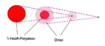
Figure 1: A pictorial representation of the exact homotopy sequence, (28), with the leftmost figure corresponding to $\pi_{2}(G/H)$.

The exact sequence (28) assumes an important significance when we consider the system with a hierarchical symmetry breaking (24),

$$G\,\,\,{\stackrel{{\scriptstyle v_{1}}}{{\longrightarrow}}}\,\,\,H\,\,\,{\stackrel{{\scriptstyle v_{2}}}{{\longrightarrow}}}\,\,\,{\bf 1}.$$

As $H$ is now completely broken the low-energy theory has vortices, classified by $\pi_{1}(H)$. If $\pi_{1}(G)={\bf 1}$, however, the full theory cannot have vortices. This apparent paradox is solved when one realizes that there is another related paradox: monopoles representing $\pi_{2}(G/H)$ cannot be stable, because in the full theory the gauge group is completely broken, $G\to{\bf 1}$, and because for any Lie group, $\pi_{2}(G)={\bf 1}.$ These paradoxes solve themselves: the vortices of the low-energy theory end at the monopoles, which have large but finite masses. Or they are broken in the middle by (though suppressed) monopole-antimonopole pair production. Vice versa, the monopoles are not stable as its flux is carried away by the vortex. See Fig. 2

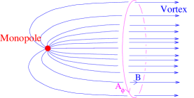
Figure 2:

Applied to the case of $SO(3)\to U(1)\to{\bf 1}$, this was precisely the logic used by ’t Hooft in his pioneering paper on the monopoles. As is seen from Fig. 1, the vortices ($\pi_{1}(U(1))=\mathbf{Z}$) of the winding number two, corresponding to the trivial element of $\pi_{1}(SO(3))={\mathbf{Z}}_{2}$, should not be stable in the full theory: there must be a regular monopole-like configuration, having the magnetic charge twice the Dirac unit, $g_{m}={4\pi}/{g}$, where $g$ is the the gauge coupling constant of the $SO(3)$ theory, acting as a source or a sink of the magnetic flux (Fig. 2).

An important new aspect we have here, as compared to the case discussed by ’t Hooft [2] is that now the unbroken group $H$ is non-Abelian and that the low-energy vortices carry continuous, non-Abelian flux moduli. As the color-flavor diagonal symmetry $H_{C+F}$ is an exact unbroken symmetry of the full theory, and the non-Abelian moduli among the low-energy vortices is a consequence of it, it follows that the the monopoles appearing as the endpoints of such vortices carry the same continuous moduli.

The monopole transformation properties follow from those of the vortices, which can be studied exactly in the low-energy approximation.

5 ${\cal N}=2$ supersymmetric gauge theories and light non-Abelian monopoles

It is always a healthy attitude to try to test one’s general idea against a concrete model. For various reasons it turns out that ${\cal N}=2$ models provides a good testing ground, as the results of strong infrared dynamics are known in the form of exact Seiberg-Witten curves. Another advantage is that by varying certain parameters upon which the system depends holomorphically, as is usual in supersymmetric theories, one can study the system Eq. (8) in different regimes.

In the regions of parameters where $v_{1}\gg v_{2}\gg\Lambda$, semiclassical analysis in the original electric theory is justified, and one can study monopoles (in the effective theory at mass scales much higher than $v_{2}$) and separately, the vortices (in the effective theory valid at mass scales much lower than $v_{1}$). The symmetry and homotopy-map argument allows to obtain the missing information about the non-Abelian transformation properties of the monopoles, from the known properties of the vortices. We come back to this discussion in Section 7.2. In the concrete models studied there the breaking mass scales are given by $m_{i}=m\sim v_{1}$; $\sqrt{\mu\,m}\sim v_{2}$, so the parameter regions explored correspond to $|m_{i}|\gg|\mu|\gg\Lambda$.

These results are then checked against the fully quantum mechanical results on the monopoles appearing as the massless degrees of freedom in the magnetic dual theory, in the region $v_{1}\sim v_{2}\sim\Lambda$. This regime will be discussed first. In the following Section 5.2, in fact, the parameters are chosen to be $m_{i},\mu\sim\Lambda$, and in particular, $m_{i}\to m$.

We shall return later (Section 7.2) to see that how our ideas on non-Abelian duality based on the hierarchical symmetry breaking and on color-flavor diagonal symmetry can be studied in the same model reliably and see that the results found match the full quantum results.

5.1 Seiberg-Witten solution of pure ${\cal N}=2$ Yang-Mills

${\cal N}=2$ supersymmetric $SU(2)$ Yang-Mills theory is described by the Lagrangian,

$$L=\frac{1}{8\pi}\hbox{\rm Im}\,\tau_{cl}\left[\int d^{4}\theta\,\Phi^{\dagger}e^{V}\Phi+\int d^{2}\theta\,\frac{1}{2}WW\right]$$ (29)

where

$$\tau_{cl}\equiv\frac{\theta_{0}}{2\pi}+\frac{4\pi i}{g_{0}^{2}}$$ (30)

is the bare $\theta$ parameter and coupling constant. $\Phi=\phi\,+\,\sqrt{2}\,\theta\,\psi+\,\ldots\,$, and $W_{\alpha}=-i\lambda\,+\,\frac{i}{2}\,(\sigma^{\mu}\,{\bar{\sigma}}^{\nu})_{\alpha}^{\beta}\,F_{\mu\nu}\,\theta_{\beta}+\,\ldots$ are ${\cal N}=1$ chiral and gauge superfields, both in the adjoint representation of the gauge group. The theory possesses ${\cal N}=2$ supersymmetry as there are two gauginos, $\lambda$ and $\psi$.

The scalar potential in this case is just the so-called $D$ term

$$V_{D}=\frac{g^{2}}{8}|[\Phi^{\dagger},\Phi]|^{2},$$ (31)

only, and the system has a continuous vacuum degeneracy (CMS- classical moduli space), parametrized by a complex number $a$,

$$\langle\Phi\rangle=\left(\begin{array}[]{cc}a&0\\ 0&-a\end{array}\right).$$ (32)

At any given $a$ the gauge symmetry is broken by Higgs mechanism to $U(1)$. The low energy theory is a $U(1)$ theory, describing the photon and photino $\lambda$, and the ${\cal N}=2$ partners, $A=(A,\psi)$.

The general requirement of ${\cal N}=2$ supersymmetry implies that the Lagrangian has the form,

$$L_{eff}=\frac{1}{4\pi}\hbox{\rm Im}\,[\int d^{4}\theta\frac{dF(A)}{dA}\,{\bar{A}}+\int\frac{1}{2}\frac{d^{2}F(A)}{dA^{2}}\,W^{\alpha}\,W_{\alpha}\,],$$ (33)

with $F(A)$ is holomorphic in $A$. $F(A)$ is known as prepotential. Going to component fields, the fermionic and gauge parts take the form,

$$L_{ferm}=\frac{1}{8\pi^{2}}[\hbox{\rm Im}\frac{d^{2}F(A)}{dA^{2}}](i{\bar{\psi}}{\bar{\sigma}}^{\mu}{\bar{D}}_{\mu}\psi+i{\bar{\lambda}}{\bar{\sigma}}^{\mu}{\bar{D}}_{\mu}\lambda+\ldots),$$

$$L_{gauge}=\frac{1}{16\pi^{2}}[\hbox{\rm Im}\frac{d^{2}F(A)}{dA^{2}}](F_{\mu\nu}^{2}+i\,F_{\mu\nu}\,{\tilde{F}}^{\mu\nu}+\ldots),$$

which shows clearly $\psi$ and $\lambda$ have the same properties as the adjoint fermions ($SU_{R}(2)$ global symmetry of ${\cal N}=2$ supersymmetry); the second formula shows that

$$\tau_{eff}=\frac{dA_{D}}{dA}=\frac{d^{2}F(A)}{dA^{2}},\qquad A_{D}\equiv\frac{dF(A)}{dA},$$

acts as the low-energy effective (complex) coupling constant

$$\tau_{eff}=\frac{\theta_{eff}}{2\pi}+\frac{4\pi i}{g_{eff}^{2}},$$ (34)

Let us recall that in general $4D$ supersymmetric sigma model, with a set of scalar multilpets $\Phi$, the kinetic term is given by a (real) Kähler potential

$$L=\int d^{4}\theta\,K(\Phi,{\bar{\Phi}})=\frac{\partial^{2}K}{\partial\phi_{i}\,\partial{\bar{\phi}}_{j}}\,\partial_{\mu}\phi_{i}\,\partial^{\mu}{\bar{\phi}}_{j}+\ldots.$$

Here the Kähler potential has a special form, determined by the prepotential,

$$K=\frac{1}{2i}[\,\frac{dF(A)}{dA_{i}}\,{\bar{A}}_{i}-\frac{dF({\bar{A}})}{d{\bar{A}}_{i}}\,{A}_{i}\,]$$

(termed special geometry).

Coming back to the $SU(2)$ ${\cal N}=2$ Yang-Mills theory where there is only one scalar multiplet $A$, the bosonic part of the Lagrangian has the form,

$$L_{bos}=\frac{1}{2\,i}\,(\partial_{\mu}\,a_{D}\,\partial^{\mu}{\bar{a}}-\partial_{\mu}\,a\,\partial^{\mu}{\bar{a}}_{D})+\hbox{\rm Im}\tau(a)(F_{\mu\nu}^{+})^{2},\qquad F_{\mu\nu}^{+}=F_{\mu\nu}+i\,{\tilde{F}}_{\mu\nu}.$$

Now this model has a nice property of (form) invariance under the generalized electromagnetic duality transformation [40]

$$\left(\begin{array}[]{c}a_{D}\\ a\end{array}\right)\to M\,\left(\begin{array}[]{c}a_{D}\\ a\end{array}\right),\qquad\left(\begin{array}[]{c}F_{\mu\nu}^{+}\\ G_{\mu\nu}^{+}\end{array}\right)\to M\,\left(\begin{array}[]{c}F_{\mu\nu}^{+}\\ G_{\mu\nu}^{+}\end{array}\right);$$ (35)

where

$$G_{\mu\nu}^{+}\equiv\frac{1}{2}\frac{\partial}{\partial F_{\mu\nu}^{+}}\,[\tau(a)\,F_{\mu\nu}^{+\,{2}}]$$

and $M$ is an $SL(2,Z)$ matrix,

$$M=\left(\begin{array}[]{cc}A&B\\ C&D\end{array}\right),\qquad A\,D-B\,C=1.$$

Such an invariance group includes the electromagnetic duality transformation $F_{\mu\nu}\leftrightarrow{\tilde{F}}_{\mu\nu}$, together with $a\leftrightarrow a_{D}$.

Since $F(A)$ is holomorphic, so is $\tau(A)$: it is harmonic, $\nabla\tau=\nabla\hbox{\rm Im}\tau=0.$ Thus $\hbox{\rm Im}\tau$ cannot be everywhere positive. This means that $A$ cannot be a good global variable everywhere in the field space: there must be some singularities where the description in terms of $a$, $F_{\mu\nu}$ fails.

The beautiful argument by Seiberg and Witten [23, 24] that the singularity be related to the point where the magnetic monopole of the theory – as the bosonic part of the model is just the Giorgi-Glashow model the soliton monopoles found by ’t Hooft and Polyakov are part of the spectrum – becomes massless due to quantum effects, and the consequent determination of the the prepotential $F(A)$ are by now well known. For completeness we summarize the main points of the solution in Appendix C. Let us recall the main result here: by introducing an auxiliary torus (whose genus $1$ corresponds to the rank of the gauge group $SU(2)$), described by the algebraic curve

$$y^{2}=(x^{2}-\Lambda^{4})(x-u)=(x+\Lambda^{2})(x-\Lambda^{2})(x-u),\qquad u\equiv\langle{\rm Tr}\Phi^{2}\rangle,$$ (36)

the solution is expressed as

$$\frac{da_{D}}{du}=\oint_{\beta}\frac{dx}{y},\qquad\frac{da}{du}=\oint_{\alpha}\frac{dx}{y},$$ (37)

where $\alpha$ and $\beta$ are the two canonical cycles on the torus, Fig. 3.

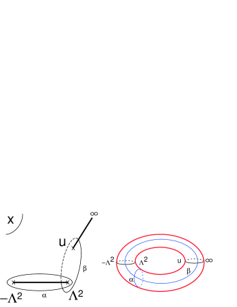
Figure 3: The torus (36) represented as a two-sheeted Riemann surfaces, with two branch cuts (left). Note that two Riemann spheres attached at two cuts are equivalent to a torus (figure on the right).

Explicitly,

$$a_{D}(u)=\frac{\sqrt{2}}{\pi}\int_{\Lambda^{2}}^{u}\left(\frac{x-u}{x^{2}-\Lambda^{4}}\right)^{1/2}=i\,\frac{u-\Lambda^{2}}{2}\,F(\frac{1}{2},\frac{1}{2};2;\frac{\Lambda^{2}-u}{2}),$$

$$a(u)=\frac{\sqrt{2}}{\pi}\int_{\Lambda^{2}}^{\Lambda^{2}}\left(\frac{x-u}{x^{2}-\Lambda^{4}}\right)^{1/2}=\sqrt{2}\,(u+\Lambda^{2})^{1/2}\,F(-\frac{1}{2},\frac{1}{2};1;\frac{2}{u+\Lambda^{2}}).$$ (38)

The key step of the solution Eq. (37) was the theorem in algebraic geometry that the integrals of the holomorphic differential ($\frac{dx}{y}$ in our case of the genus one torus (36)) along the canonical cycles $\alpha$ and $\beta$ (they are called period integrals) satisfy

$$\hbox{\rm Im}\frac{\oint_{\alpha}\frac{dx}{y}}{\oint_{\beta}\frac{dx}{y}}>0,$$

independently of the way canonical cycles are redefined. According to the identification of the period integrals with the physical quantities as Eq. (37) this guarantees that

$$\hbox{\rm Im}\,\tau_{eff}=\hbox{\rm Im}\frac{da_{D}}{da}=\frac{4\pi}{g_{eff}^{2}}>0.$$

Let us add several remarks.

(i)

Another key observation by Seiberg-Witten is that the ${\cal N}=2$ supersymmetry implies an exact mass formula for BPS saturated states with magnetic and electric charges $n_{m},n_{e}$:

$$M_{n_{m},n_{e}}=\sqrt{2}\,|n_{m}\,a_{D}+n_{e}\,a|.$$ (39)

This is a consequence of the fact that the system has an underlying ${\cal N}=2$ supersymmetry with a central extension. See Appendix D. This formula generalizes the standard Higgs formula, $M_{0,n_{e}}=g\,n_{e}\langle\phi\rangle$, as $a\sim g\langle\phi\rangle$ semiclassically, and at the same time, the ’t Hooft-Polyakov monopole mass formula, $M_{n_{m},0}=4\,\pi\,n_{m}\,\langle\phi\rangle/g$ (semiclassically $a_{D}\sim 4\,\pi\,\langle\phi\rangle/g$). Note that in the fully quantum formula (39) the magnetic and electric charges appear symmetrically. Indeed the mass formula is invariant under the generalized duality transformations (35), modulo appropriate relabeling of magnetic and electric charges.

(ii)

Quite remarkably the low-energy effective action thus determined contains quantum effects in its entirety, the one-loop perturbative effects plus the sum of infinite instanton contributions. Indeed, the Seiberg-Witten curves have been checked against direct instanton calculations [41], and more recently, have been rederived by an explicit instanton resummation [42].

(iv)

The Seiberg-Witten solution nicely solves an old (apparent) paradox related to the Dirac quantization versus renormalization group [8]: how can the relation $g_{m}\,g_{e}=2\,\pi\,n$, $n=0,1,\ldots$ be compatible with the fact that both the electric and magnetic charges are Abelian $U(1)$ coupling constants, expected to get renormalized in the same direction? In the Seiberg-Witten solution, $g_{m}(\mu)$ gets renormalized as in (magnetic version of) QED, through monopole loops, with monopoles replacing the role of the electron. The same infrared behavior is explained, in the original electric picture, as due to instanton-induced nonperturbative renormalization of the electric coupling constant $g_{e}(\mu)$. As a consequence $g_{m}(\mu)\,g_{e}(\mu)=4\,\pi$ holds [23] at any infrared cutoff $\mu=\langle a_{D}\rangle.$ For other subtle issues related to renormalization group properties of Seiberg-Witten solution, see [43].

(iv)

How do we know that these massless monopoles are related to the ’t Hooft-Polyakov monopoles? That they are indeed them, can be verified by studying the electric and quark (in the cases with $N_{f}=1,2,3$) number charges. As is well known the ’t Hooft-Polyakov monopoles acquire these $U(1)$ charges quantum mechanically, via a beautiful phenomenon of charge fractionalization [44], which in this specific situation are the Witten’s [45] and Jackiw-Rebbi’s effects [46]. By moving within the space of vacua (QMS) and going into the regions where semiclassical approximation is valid (where $u=\langle{\rm Tr}\,\Phi^{2}\rangle\gg\Lambda^{2}$), one can compare these fractional $U(1)$ charges read off from the leading terms of the exact Seiberg-Witten solution with the ones obtained many years earlier by standard quantization of fermion fields around the semiclassical monopole backgrounds [47]. The results exactly match [48, 49, 50].

(iv)

The low-energy effective Lagrangian near one of the singularities, e.g., $u=\Lambda^{2}$, looks like a (dual) QED with a massless monopole, whose Lagrangian has the standard ${\cal N}=2$ QED form,

$$L = \frac{1}{4\pi}\hbox{\rm Im}\,[\int d^{4}\theta\frac{dF(A_{D})}{dA_{D}}\,{\bar{A}_{D}}+\int\frac{1}{2}\frac{d^{2}F(A_{D})}{dA_{D}^{2}}\,W_{D}^{\alpha}\,W_{D\,\alpha}\,]+$$ (40)

$$+\int d^{4}\theta({\bar{M}}e^{V_{D}}M+{\tilde{M}}e^{-V_{D}}{\bar{\tilde{M}}})+\int d^{2}\theta\sqrt{2}{\tilde{M}}A_{D}M,$$

where the gauge terms are just the dual of Eq. (33); the third and fourth terms describe the monopole.

(v)

Addition of a ${\cal N}=1$ perturbation, the adjoint scalar mass term, $\mu\,{\rm Tr}\Phi^{2}$ in the original electric theory induces $\Delta L=\mu\,U(A_{D}),$ where the function $U(A_{D})$ is the inverse of the solution $a_{D}(u)$. By minimizing the potential, the degeneracy (quantum moduli space – QMS) is eliminated leaving just two vacua, where

$$a_{D}=0,\quad u=\langle{\rm Tr}\Phi^{2}\rangle=\pm\Lambda^{2},\qquad\langle M\rangle=\langle{\tilde{M}}\rangle=\mu\,\frac{\partial U}{\partial A_{D}}\sim\mu\,\Lambda.$$

The first result says that the magnetic monopole is massless in this vacuum (see Eq. (40)), the third states that the magnetic monopole condenses, leading to confinement à la ’t Hooft-Mandelstam. This is perhaps the first example of nontrivial 4D system where this phenomenon has been demonstrated explicitly and analytically.

5.2 Seiberg-Witten solutions for ${\cal N}=2$ models with quarks

A general enthusiasm (alarm?) caused by the news that the $SU(2)$ Seiberg-Witten model with a small ${\cal N}=1$ perturbation exhibited the ’t Hooft-Mandelstam mechanism of confinement, was followed by a widespread delusion (relief?) among theoretical physicists when it was realized that the light monopoles appearing in the low-energy theory were Abelian and at the same time confinement was accompanied by dynamical Abelianization. This surely was not a good model of QCD! The fact that in the $SU(2)$ models with $N_{f}=1,2,3$ hypermultiplets of quarks, studied in the (quite remarkable) second paper by Seiberg and Witten [24], as well as in pure ${\cal N}=2$ Yang-Mills theories with more general gauge groups [25], the low-energy monopoles were always Abelian, did not help.

What was not realized at the time, however, was the fact that there was a clear reason for the Abelianization in these simplest models (see Subsection 5.3 below), and that, in the context of a more general class of ${\cal N}=2$ theories with quark multiplets, Abelian confinement belonged to the exceptional cases. In fact, confinement is more typically caused by condensation of non-Abelian monopoles, as the subsequent analyses have revealed. We shall below briefly summarize the main features of these models, with technical aspects kept at its minimum.

The systems we consider are simple generalization of the ${\cal N}=2$ models with “quark” multiplets. The $N=1$ chiral and gauge superfields $\Phi=\phi\,+\,\sqrt{2}\,\theta\,\psi+\,\ldots\,$, and $W_{\alpha}=-i\lambda\,+\,\frac{i}{2}\,(\sigma^{\mu}\,{\bar{\sigma}}^{\nu})_{\alpha}^{\beta}\,F_{\mu\nu}\,\theta_{\beta}+\,\ldots$ are both in the adjoint representation of the gauge group, while the hypermultiplets are taken in the fundamental representation of the gauge group. The Lagrangian takes the form,

$$L=\frac{1}{8\pi}\hbox{\rm Im}\,\tau_{cl}\left[\int d^{4}\theta\,\Phi^{\dagger}e^{V}\Phi+\int d^{2}\theta\,\frac{1}{2}WW\right]+L^{(quarks)}+\Delta L+\Delta^{\prime}L,$$ (41)

$$L^{(quarks)}=\sum_{i}\,[\int d^{4}\theta\,\{Q_{i}^{\dagger}e^{V}Q_{i}+{\tilde{Q}_{i}}^{\dagger}e^{{\tilde{V}}}{\tilde{Q}}_{i}\}+\int d^{2}\theta\,\{\sqrt{2}{\tilde{Q}}_{i}\Phi Q^{i}+m_{i}{\tilde{Q}}_{i}Q^{i}\}$$ (42)

describes the $n_{f}$ flavors of hypermultiplets (“quarks”),

$$\tau_{cl}\equiv\frac{\theta_{0}}{\pi}+\frac{8\pi i}{g_{0}^{2}}$$ (43)

is the bare $\theta$ parameter and coupling constant. The $N=1$ chiral and gauge superfields $\Phi=\phi\,+\,\sqrt{2}\,\theta\,\psi+\,\ldots\,$, and $W_{\alpha}=-i\lambda\,+\,\frac{i}{2}\,(\sigma^{\mu}\,{\bar{\sigma}}^{\nu})_{\alpha}^{\beta}\,F_{\mu\nu}\,\theta_{\beta}+\,\ldots$ are both in the adjoint representation of the gauge group, while the hypermultiplets are taken in the fundamental representation of the gauge group.

We consider small generic nonvanishing bare masses $m_{i}$ for the hypermultiplets (“quarks”), which is consistent with ${\cal N}=2$ supersymmetry. Furthermore it is convenient to introduce the mass for the adjoint scalar multiplet

$$\Delta L=\int\,d^{2}\theta\,\mu\,{\rm Tr}\,\Phi^{2}$$ (44)

which breaks supersymmetry to ${\cal N}=1$. An advantage of doing so is that all flat directions are eliminated and one is left with a finite number of isolated vacua; keeping track of this number (and the symmetry breaking pattern in each of them) allows us to make highly nontrivial check of our analyses at various stages.

Below we summarize the physical results on these systems. To solve the system (41) the first step is the generalization of the curve Eq. (36) to the case of general group $G$. When the breaking is maximum, $G\to U(1)^{r_{G}}$ where $r_{G}$ is the rank of the group $G$, we set $\mu=0$ and consider vacua

$$\langle\Phi\rangle=\hbox{\rm diag}(\phi_{1},\phi_{2},\ldots),\qquad\phi_{1}\neq\phi_{2},\quad etc.$$ (45)

The auxiliary genus $g=N_{c}-1$ (or $N_{c}$) curves for $SU(N_{c})$ ($USp(2N_{c})$) theories corresponding to these classical vacua (called Coulomb branch of the moduli space) are given by

$$y^{2}=\prod_{k=1}^{n_{c}}(x-\phi_{k})^{2}+4\Lambda^{2n_{c}-n_{f}}\prod_{j=1}^{n_{f}}(x+m_{j}),\qquad SU(N_{c}),\,\,\,N_{f}\leq 2N_{c}-2,$$ (46)

and

$$y^{2}=\prod_{k=1}^{n_{c}}(x-\phi_{k})^{2}+4\Lambda\prod_{j=1}^{n_{f}}\left(x+m_{j}+\frac{\Lambda}{N_{c}}\right),\qquad SU(N_{c}),\,\,\,N_{f}=2N_{c}-1,$$ (47)

with $\phi_{k}$ subject to the constraint $\sum_{k=1}^{n_{c}}\phi_{k}=0$, and

$$xy^{2}=\left[x\prod_{a=1}^{n_{c}}(x-\phi_{a}^{2})^{2}+2\Lambda^{2n_{c}+2-n_{f}}m_{1}\cdots m_{n_{f}}\right]^{2}-4\Lambda^{2(2n_{c}+2-n_{f})}\prod_{i=1}^{n_{f}}(x+m_{i}^{2})$$ (48)

for $USp(2N_{c})$. Analogous results for $SO(N_{c})$ theories are also known.

The connection between these genus $g$ hypertori and physics is made [23]-[29] through the identification of various period integrals of the holomorphic differentials on the curves with $(da_{Di}/du_{j},da_{i}/du_{j})$, where the gauge invariant parameters $u_{j}$’s are defined by the standard relation,

$$\prod_{a=1}^{n_{c}}(x-\phi_{a})=\sum_{k=0}^{N_{c}}u_{k}\,x^{N_{c}-k},\qquad u_{0}=1,\quad u_{1}=0,\qquad SU(N_{c});$$ (49)

$$\prod_{a=1}^{n_{c}}(x-\phi_{a}^{2})=\sum_{k=0}^{N_{c}}u_{k}\,x^{N_{c}-k},\qquad u_{0}=1,\qquad USp(2N_{c}),$$ (50)

and $u_{2}\equiv\langle{\rm Tr}\,\Phi^{2}\rangle,$ $u_{3}\equiv\langle{\rm Tr}\,\Phi^{3}\rangle,$ etc. The VEVS of $a_{Di},\,\,a_{i}$, which are directly related to the physical masses of the BPS particles through the exact Seiberg-Witten mass formula [23, 24]

$$M^{n_{mi},n_{ei},S_{k}}=\sqrt{2}\,\left|\sum_{i=1}^{g}(n_{mi}\,a_{Di}+n_{ei}\,a_{i})+\sum_{k}S_{k}m_{k}\right|,$$ (51)

are constructed as integrals over the non-trivial cycles of the meromorphic differentials on the curves. $S_{k}$ are the $i$-th quark number charge of the monopole under consideration, which enters the formula for the central charges (hence the mass).

(i)

These formulae naturally generalize those of the pure $SU(2)$ theory, Eq. (37), Eq. (39). The singularities of the curves Eq. (46)-Eq. (48) are the points in the space of vacua (QMS) where various particles become massless.

(ii)

When $m_{i}\gg\Lambda$ these singularities are at the points where $\phi\sim m_{i}$ (where the quarks become massless – see Eq. (42)) and at the points where monopoles of pure Yang-Mills theory become massless. The latter are the points the curve of the Yang-Mills theory,

$$y^{2}=\prod_{k=1}^{n_{c}}(x-\phi_{k})^{2}+4\Lambda_{YM}^{2n_{c}}$$

become maximally singular, $\sim\prod_{i=1}^{n_{c}-1}(x-x_{i})^{2}(x-\alpha)(x-\beta)$.

(iii)

It is the property of these curves that when $m_{i}\sim\Lambda$ all singularities are found to correspond to magnetic degrees of freedom (massless monopoles and dyons). To trace how, as $m_{i}$ are varied, the original “electric” singularities (massless quarks) make a metamorphosis into magnetic monopoles, due to the movement of certain branch points (or branch cuts) sliding under other branch cuts (branch surfaces), is a rather complicated business, and has been analyzed satisfactorily only in the $SU(2)$ theories with matter [24, 51].

(iv)

The particular form of the curve specific to different groups reflect different global symmetries. A nice discussion is given in [26].

5.3 Exact quantum behavior of light non-Abelian monopoles

Physics of confining vacua and properties of light monopoles in these theories are studied by identifying all of the ${\cal N}=1$ vacua (the points in the QMS – quantum moduli space, that is, the space of vacua – which survive the ${\cal N}=1$ perturbation) and studying the low-energy action for each of them. The underlying ${\cal N}=2$ theory, especially with $m_{i}=0$ or with equal masses $m_{i}=m$, has a large continuous degeneracy of vacua (flat directions), which has been studied by using the Seiberg-Witten curves, non-renormalization of Higgs branch metrics, superconformal points and their universality, their moduli structure and symmetries, etc [28, 29]. For the purpose of this section, however, we are most interested in the set of vacua which are picked up when the small generic bare quark masses $m_{i}$ and a small nonzero adjoint mass $\mu$ are present.

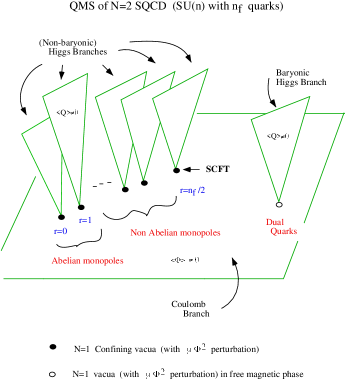
Figure 4:

At the roots of these different branches of ${\cal N}=2$ vacua where the Higgs branches meet the Coulomb branch, lie all these vacua, which survives the ${\cal N}=1$ perturbation, Eq. (44). In $SU(N_{c})$ theories with $N_{f}$ flavors with generic masses, all ${\cal N}=1$ vacua arising this way have been completely classified [30, 31].

For nearly equal quark masses they fall into classes $r=0,1,\ldots,\frac{N_{f}}{2}$ groups of vacua near the “root of non-baryonic Higgs branches”, and for $N_{f}\geq N_{c}$, there are special vacua at the “roots of baryonic Higgs branches”. These names reflect the fact that in the respective Higgs branch non-baryonic or baryonic squark VEVS,

$$\langle Q_{i}^{a}\,{\tilde{Q}}_{a}^{j}\rangle,\qquad\langle\epsilon_{a_{1}\,a_{2}\,\ldots,a_{N_{c}}}Q_{i_{1}}^{a_{1}}Q_{i_{2}}^{a_{2}}\ldots Q_{i_{N_{c}}}^{a_{N_{c}}}\rangle,$$ (52)

are formed. See Fig. 4. Each group of vacua coalesce in single vacua where the gauge symmetry is enhanced into non-Abelian gauge groups, as in Table 1, taken from Argyres et. al. [28].

The vacua at the root of the baryonic branch are in “free-magnetic” phase; the light non-Abelian magnetic monopoles appear as asymptotic states; they do not condense, no confinement and no symmetry-breaking occur. Although the appearance of the Seiberg dual gauge group, $SU({\tilde{N}}_{c})$, ${\tilde{N}}_{c}\equiv N_{f}-N_{c}$ is certainly intriguing [28], these are not type of vacua we are interested in.

Our main interest is the first classes of the so-called “$r$-vacua”, where the magnetic gauge group is

$$U(r)\times U(1)^{N_{c}-r},$$

and the massless matter multiplets consist of $N_{f}$ monopoles in the fundamental representation of $U(r)$, and flavor-singlet Abelian monopoles carrying a single charge, each with respect to one of the $U(1)$ factors (Table 1) .

	$SU(r)$	$U(1)_{0}$	$U(1)_{1}$	$\ldots$	$U(1)_{n_{c}-r-1}$	$U(1)_{B}$
$n_{f}\times q$	${\underline{\bf r}}$	$1$	$0$	$\ldots$	$0$	$0$
$e_{1}$	${\underline{\bf 1}}$	0	1	…	$0$	$0$
$\vdots$	$\vdots$	$\vdots$	$\vdots$	$\ddots$	$\vdots$	$\vdots$
$e_{n_{c}-r-1}$	${\underline{\bf 1}}$	0	0	$\ldots$	1	0

Table 1: The effective degrees of freedom and their quantum numbers at the “nonbaryonic root”.

Once the gauge group and the quantum numbers of the matter fields are all known, the ${\cal N}=2$ supersymmetry uniquely fixes the structure of the effective action. We find that

(i)

We see the non-Abelian monopoles in action, in the generic $r$ ($2\leq r\leq\frac{N_{f}}{2}$) vacua. See Table 2 taken from [30]. They behave perfectly as point-like particles, albeit in a dual, magnetic gauge system. Upon ${\cal N}=1$ perturbation they condense (confinement phase) $\langle q_{a}^{i}\rangle\sim\delta_{a}^{i}\sqrt{\mu\,\Lambda}$ and induces flavor symmetry breaking

$$SU(N_{f})\times U(1)\to U(r)\times U(N_{f}-r).$$

(ii)

The upper limit $r\leq\frac{N_{f}}{2}$ is a manifestation of monopole dynamics: only in this range of $r$ the non-Abelian monopoles can appear as recognizable infrared degrees of freedom. We now see why in the $SU(2)$ Seiberg-Witten models, as well as in pure ${\cal N}=2$ Yang-Mills (ı.e., $N_{f}=0$) models with different gauge groups, the low-energy monopoles were found to be always Abelian: in all these cases, non-Abelian monopoles would interact too strongly, not enough of them being there. We remind the reader that the beta function in ${\cal N}=2$ $SU$ theories has the pure one-loop form with $\beta_{0}\propto 2\,r-N_{f}$.

(iii)

Indeed, there are homotopy and symmetry arguments [30, 52] which suggest that non-Abelian monopoles appearing in the $r$-vacua are “baryonic constituents” of an Abelian (’t Hooft-Polyakov) monopople,

$$Abelian\,\,monopole\sim\epsilon^{a_{1}\ldots a_{r}}{q_{a_{1}}^{i_{1}}q_{a_{2}}^{i_{2}}\ldots q_{a_{r}}^{i_{r}}},$$ (53)

$a_{i}$ being the dual color indices, and $i_{m}$ the flavor indices. The $SU(r)$ gauge ineractions, being infrared-free, are unable to keep the Abelian monopole bound: they disintegrate into non-Abelian monopoles.

(iv)

That the effective degrees of freedom in the $r$ vacua are non-Abelian rather than Abelian monopoles, is actually required also by symmetry of the system [30, 53], not only from the dynamics. If the Abelian monopoles of the $r$-th tensor flavor representation were the correct degrees of freedom, the low-energy effective theory would have too large an accidental symmetry – $SU({N_{f}\choose r})$. The condensation of such monopoles would produce far-too-many Nambu-Goldstone bosons than expected from the symmetry of the underlying theory. The system prevents such an awkward situation from being realized in an elegant manner, introducing smaller solitons, non-Abelian monopoles, in the fundamental representation of the $SU(N_{f})$ so that the low-energy theory has the right symmetry.

(v)

An analogous argument might be used in the standard QCD, to exclude Abelian picture of confinement, though admittedly this is not a very rigorous one. We know from lattice simulations of $SU(3)$ theory that confinement and chiral symmetry breaking are closely related. If Abelian ’t Hooft-Monopole-Mandelstam monopoles were the right degrees of freedom describing confinement, their condensation would somehow have to describe chiral symmetry breaking as well. We would then be led to assume that they carry flavor quantum numbers of $SU(N_{f})_{L}\times SU(N_{f})_{R}$, e.g.,

$$Monopoles\sim M_{i}^{j},\qquad\langle M_{i}^{j}\rangle\propto\delta_{i}^{j}\,\Lambda_{QCD},$$

where $i,j$ are $SU(N_{f})_{L}\times SU(N_{f})_{R}$ indices. But such a system would have a far-too large accidental symmetry. Confinement would be accompanied by a large number of unexpected (and indeed unobserved) light Nambu-Goldstone bosons.

(vi)

The limiting case of $r$ vacua, with $r=\frac{N_{f}}{2}$, as well as the massless ($m_{i}\to 0$) limit of $USp(2N_{c})$ and $SO(N_{c})$ theories, are of great interest. The low-energy effective theory in these cases turn out to be conformally invariant (nontrivial infrared-fixed-point) theories. This is an analogue of an Abelian superconformal vacuum found first in the pure $SU(3)$ Yang Mills theory by Argyres and Douglas [54]. It can be explicitly checked that the low-energy degrees of freedom include relatively non-local monopoles and dyons [30, 55, 53]. There are no local effective Lagrangians describing the infrared dynamics. These are the most difficult cases to analyze, but are potentially the most interesting ones, from the point of view of understanding QCD. We shall come back to these (perhaps, crucial) cases at the end of the lecture, Section 8.

label ($r$)	Deg.Freed.	Eff. Gauge Group	Phase	Global Symmetry
$0$	monopoles	$U(1)^{n_{c}-1}$	Confinement	$U(n_{f})$
$1$	monopoles	$U(1)^{n_{c}-1}$	Confinement	$U(n_{f}-1)\times U(1)$
$\leq[\frac{n_{f}-1}{2}]$	NA monopoles	$SU(r)\times U(1)^{n_{c}-r}$	Confinement	$U(n_{f}-r)\times U(r)$
${n_{f}/2}$	rel. nonloc.	-	Confinement	$U({n_{f}/2})\times U({n_{f}/2})$
BR	NA monopoles	$SU({\tilde{n}}_{c})\times U(1)^{n_{c}-{\tilde{n}}_{c}}$	Free Magnetic	$U(n_{f})$

Table 2: Phases of $SU(n_{c})$ gauge theory with $n_{f}$ flavors. ${\tilde{n}}_{c}\equiv n_{f}-n_{c}$.

	Deg.Freed.	Eff. Gauge Group	Phase	Global Symmetry
1st Group	rel. nonloc.	-	Confinement	$U(n_{f})$
2nd Group	dual quarks	$USp(2{\tilde{n}}_{c})\times U(1)^{n_{c}-{\tilde{n}}_{c}}$	Free Magnetic	$SO(2n_{f})$

Table 3: Phases of $USp(2n_{c})$ gauge theory with $n_{f}$ flavors with $m_{i}\to 0$. ${\tilde{n}}_{c}\equiv n_{f}-n_{c}-2$.

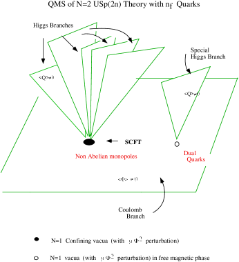
Figure 5:

6 Vortices

The moral of the story is that the non-Abelian monopoles do exist in fully quantum mechanical systems. In typical confining vacua in supersymmetric gauge theories they are the relevant infrared degrees of freedom. Their condensation induces confinement and dynamical symmetry breaking. This brings us back to the problem of understanding these light, magnetic degrees of freedom as quantum solitons:

What are their semi-classical counterparts?

Are they Goddard-Nuyts-Olive-Weinberg monopoles?

In which sense condensation of non-Abelian monopoles imply confinement?

How has the difficulty related to the dual group mentioned earlier been avoided?

These are the questions we wish to answer. The idea is to take advantage of the fact that in supersymmetric theories there are parameters which can be varied, upon which the physical properties of the system depend in a holomorphic fashion. As $m_{i}$ and $\mu$ are varied, there cannot be phase transition at some $|\mu|$ or at $|m_{i}|$: the number of Nambu-Goldstone bosons and hence the pattern of the symmetry breaking, must be invariant.

6.1 Abrikosov-Nielsen-Olesen vortex

Topologically stable vortices arise when the ground states of a system have a nontrivial moduli space which is not simply connected. The best known case [56] is the Abelian gauge theory with a charged complex matter field in Higgs phase (superconductor), where the static configurations have energy density

$$H=\frac{1}{4}F_{ij}^{2}+|D_{i}\phi|^{2}+V(|\phi|),\qquad D_{i}=\partial_{i}-i\,e\,A_{i}.$$

The potential $V$ is assumed to attain its minimum at $|\phi|=v\neq 0$. The asymptotic gauge and scalar fields must be such that the field energy be finite,

$$|\phi(x)|\to v,\qquad D_{i}\phi\to 0,\qquad F_{ij}^{2}\to 0.$$

These allow for nontrivial configurations classified by an integer,

$$\pi_{1}(U(1))={\mathbf{Z}},$$

i.e., by an integer winding number $n$,

$$\phi\to e^{in\varphi}\,v,\qquad A_{\varphi}\to\frac{n}{e\rho},$$

where $\rho,\phi,z$ are the position variables of cylindrical coordinate system. At the center of the vortex $\phi(\rho=0,\varphi)=0$ in order for $\phi(\rho,\phi)$ to be a smooth configuration: the gauge symmetry is restored along the vortex core.

Depending on the potential, the vacuum can be superconductor of type II where single isolated (Abrikosov-Nielsen-Olesen) vortices are stable, type I systems where vortices stick together to form the regions of normal ground state, and finally there is the critical case between them (BPS) where vortices has no net interaction and the tension of winding number $k$ vortex is equal to $k$ times that of the minimum-winding vortex.

6.2 ${\mathbf{Z}}_{N}$ vortices

In pure $SU(N)$ theory with all matter fields in adjoint representation, the true gauge group is $\frac{SU(N)}{{\mathbf{Z}}_{N}}$. When the gauge group is completely broken the vacuum manifold has nontrivial structure,

$$\pi_{1}(\frac{SU(N)}{{\mathbf{Z}}_{N}})={\mathbf{Z}}_{N}.$$ (54)

The asymptotic behavior of the fields, required by finiteness of the tension is

$$A_{i}\sim\frac{i}{g}\,U(\phi)\partial_{i}U^{\dagger}(\phi);\quad\phi_{A}\sim U\phi_{A}^{(0)}U^{\dagger},\qquad U(\phi)=\exp{i\sum_{j}^{r}\beta_{j}T_{j}\phi}$$

where $T_{j}$ are the generators of the Cartan subalgebra of $H$, $\phi_{A}^{(0)}$ are the (set of) VEVs of the adjoint scalar fields which break the $SU(N)$ group completely. The smoothness of the configurations requires the quantization condition: ($\alpha$ = root vectors of $H$)

$$U(2\pi)\in{\bf Z}_{N},\qquad{\alpha}\cdot{\beta}\in{\bf Z}.$$ (55)

The second condition of (55) appears to imply that these vortices be characterized by the weight vectors of the group ${\tilde{H}}=SU(N)$, dual of $H=SU(N)/{\bf Z}_{N}$ [4]: one vortex for each irreducible representation of ${\tilde{H}}$. Actually, Eq. (54) shows that there is just one stable vortex with a given ${\bf Z}_{N}$ charge ($N$-ality).

An interesting model of this sort is the so-called $N=1^{*}$ theory [57, 58, 59] defined as the ${\cal N}=4$ supersymmetric theory with addition of mass terms for the three adjoint scalar multiplets,

$$\Delta L=\sum_{i=1}^{3}m_{i}\,\Phi_{i}^{2}|_{\theta\theta},$$

which break supersymmetry to ${\cal N}=1$. The general properties of chiral condensates,

$$\langle W\,W\rangle,\quad\langle\Phi_{1}^{2}\rangle,\quad\langle\Phi_{2}^{2}\rangle,\quad\langle\Phi_{3}^{2}\rangle,$$

in all possible types of vacua (confinement vacua, Coulomb vacua, Higgs vacua) have been analyzed exactly in a series of papers [60].

This model is based on the underlying ${\cal N}=4$ model, which is believed to display exact Olive-Montonen duality. In spite of the relative simplicity of the model, the properties of ${\bf Z}_{N}$ monopoles in the Higgs (or partially Higgs) vacua in the ${\cal N}=1^{*}$ are not very well known, except for the $SU(2)$ [61] or $SU(3)$ cases.

6.3 Non-Abelian vortices in a $U(N)$ model

The ${\bf Z}_{N}$ vortice discussed in the preceding section at first sight appears to carry a non-Abelian charge, being labelled by the weight vector of a non-Abelian dual group ${\tilde{H}}$: actually, they do not [62]. It is just a single solution, which can be transformed by Weyl transformations of $H$. There are no continuous moduli associated to it.

Truly non-Abelian vortices have been constructed [35, 37] in the context of a ${\cal N}=2$ supersymmetric $U(N)$ gauge theory, with $N_{f}$ flavors, where the gauge group is broken by the VEVs of a set of scalar fields in the fundamental representations. The model Lagrangian has the form

$${\cal L} = {\rm Tr}\left[-\frac{1}{2g^{2}}F_{\mu\nu}F^{\mu\nu}-\frac{2}{g^{2}}\mathcal{D}_{\mu}\,\phi^{\dagger}\,\mathcal{D}^{\mu}\phi-\mathcal{D}_{\mu}\,H\,\mathcal{D}^{\mu}H^{\dagger}-\lambda\left(c\,{\bf 1}_{N}-H\,H^{\dagger}\right)^{2}\right]$$ (56)

$$+ {\rm Tr}\,[\,(H^{\dagger}\phi-M\,H^{\dagger})(\phi\,H-H\,M)\,]$$

where $F_{\mu\nu}=\partial_{\mu}W_{\nu}-\partial_{\nu}W_{\nu}+i\left[W_{\mu},W_{\nu}\right]$ and $\mathcal{D}_{\mu}H=\left(\partial_{\mu}+i\,W_{\mu}\right)\,H$, and $H$ represents the fields in the fundamental representation of $SU(N)$, written in a color-flavor $N\times N_{f}$ matrix form, $(H)_{\alpha}^{i}\equiv q_{\alpha}^{i}$, and $M$ is a $N_{f}\times N_{f}$ mass matrix. Here, $g$ is the $U(N)_{\rm G}$ gauge coupling, $\lambda$ is a scalar coupling. For

$$\lambda=\frac{g^{2}}{4}$$ (57)

the system is BPS saturated. For such a choice, the Eq. (56) can be regarded as a truncation of the bosonic sector of an ${\cal N}=2$ supersymmetric $U(N)$ gauge theory, and with $(H)_{\alpha}^{i}$ representing the half of the squark fields,

$$(H)_{\alpha}^{i}\equiv q_{\alpha}^{i},\qquad{\tilde{q}}^{\alpha}_{i}\equiv 0$$ (58)

In the supersymmetric context the parameter $c$ is the Fayet-Iliopoulos parameter. In the following we set $c>0$ so that the system be in Higgs phase, and so as to allow stable vortex configurations. For generic, unequal quark masses,

$$M=diag\,(m_{1},m_{2},\ldots,m_{N_{f}}),$$ (59)

the adjoint scalar VEV takes the form,

$$\langle\phi\rangle=M=\left(\begin{array}[]{cccc}m_{1}&0&0&0\\ 0&m_{2}&0&0\\ 0&0&\ddots&0\\ 0&0&0&m_{N}\end{array}\right),$$ (60)

which breaks the gauge group to $U(1)^{N}$.

In order to have a non-Abelian vortex, it is necessary to choose masses equal,

$$M=diag\,(m,m,\ldots,m),$$ (61)

the adjoint and squark fields have the vacuum expectation value (VEV)

$$\langle\phi\rangle=m\,{\mathbf{1}}_{N},\qquad\langle H\rangle=\sqrt{c}\,\left(\begin{array}[]{ccc}1&0&0\\ 0&\ddots&0\\ 0&0&1\end{array}\right)$$ (62)

where only the first $N$ flavors are left explicit. The squark VEV breaks the gauge symmetry completely, while leaving an unbroken $SU(N)_{C+F}$ color-flavor diagonal symmetry (the flavor group acts on $H$ from the right while the $U(N)_{\rm G}$ gauge symmetry acts on $H$ from the left). The global symmetry group associate with the other $N_{f}-N$ flavors also remains unbroken. The BPS vortex equations are

$$\left(\mathcal{D}_{1}+i\mathcal{D}_{2}\right)\,H=0,\quad F_{12}+\frac{g^{2}}{2}\left(c\,{\bf 1}_{N}-H\,H^{\dagger}\right)=0.$$ (63)

The matter equation can be solved [65]-[67] by use of the $N\times N$ moduli matrix $H_{0}(z)$ whose components are holomorphic functions of the complex coordinate $z=x^{1}+ix^{2}$,

$$H=S^{-1}(z,\bar{z})\,H_{0}(z),\quad W_{1}+i\,W_{2}=-2\,i\,S^{-1}(z,\bar{z})\,\bar{\partial}_{z}S(z,\bar{z}).$$ (64)

The gauge field equations then take the simple form (“master equation”)

$$\partial_{z}\,(\Omega^{-1}\partial_{\bar{z}}\,\Omega)=\frac{g^{2}}{4}\,(c\,{\mathbf{1}}_{N}-\Omega^{-1}\,H_{0}\,H_{0}^{\dagger}).$$ (65)

The moduli matrix and $S$ are defined up to a redefinition,

$$H_{0}(z)\to V(z)\,H_{0}(z),\qquad S(z,\bar{z})\to V(z)\,S(z,\bar{z}),$$ (66)

where $V(z)$ is any non-singular $N\times N$ matrix which is holomorphic in $z$. This class of model has been extensively studied recently [65]-[71]. In particular, in the contex of these models a considerable attention was given to the system in which $U(N)$ gauge symmetry is either explicitly or dynamically broken to $U(1)^{N}$, producing Abelian monopoles. As the terminology used and concepts involved, though physically distinct, are often similar to the concept of non-Abelian monopoles discussed in this note, and could be misleading.

6.4 Dynamical Abelianization

As should be clear from what we said so far, it is crucial that the color-flavor diagonal symmetry $SU(N)$ remains exactly conserved, for the emergence of non-Abelian dual gauge group (see the next Section). Consider, instead, the cases in which the gauge $U(N)$ (or $SU(N)\times U(1)$) symmetry is broken to Abelian subgroup $U(1)^{N}$, either by small quark mass differences (Eq. (60)) or dynamically, as in the ${\cal N}=2$ models with $N_{f}<2\,N$ [36, 69]. From the breaking of various $SU(2)$ subgroups to $U(1)$ there appear light ’t Hooft-Polyakov monopoles of mass $O(\frac{\Delta m}{g})$ (in the case of an explicit breaking) or $O(\Lambda)$ (in the case of dynamical breaking). As the $U(1)^{N}$ gauge group is further broken by the squark VEVs, the system develops ANO vortices. The light magnetic monopoles, carrying magnetic charges of two different $U(1)$ factors, look confined by the two vortices (Fig. 6). These cases have been discussed extensively [67]-[70], within the context of $U(N)$ model of Subsection 6.3.

The dynamics of the fluctuation of the orientational modes along the vortex turns out to be described by a two-dimensional ${\bf C}P^{N-1}$ model [35, 37]. It has been shown [35, 36, 69, 70], that the kinks of the two-dimensional sigma model precisely correspond to these light monopoles, to be expected in the underlying $4D$ gauge theory. In particular, it was noted that there is an elegant matching between the dynamics of two-dimensional sigma model (describing the dynamics of the vortex orientational modes in the Higgs phase of the $4D$ theory) and the dynamics of the $4D$ gauge theory in the Coulomb phase, including the precise matching of the coupling constant renormalization [68, 36, 69].

Note that these cases are analogue of what would occur in QCD if the color $SU(3)$ symmetry were to dynamically break itself to $U(1)^{2}$. Confinement would be described in this case by the condensation of magnetic monopoles carrying the Abelian charges $Q^{1}$, or $Q^{2}$, and the resulting ANO vortices will be of two types, $1$ and $2$ carrying the related fluxes.

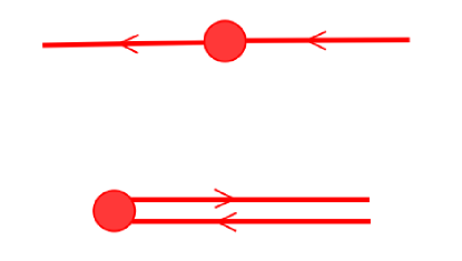
Figure 6: Monopoles in $U(N)$ systems with Abelianization are confined by two Abelian vortices.

7 The model

Actually the model we need here is not exactly the model of Section 6.3, but is a model which contains it as a low-energy approximation. It is the same model already discussed in Section 5.2, but now we analyze it in the region, $m_{i}\gg\mu\gg\Lambda$, so that the semiclassical reasoning of Section 4 makes sense. For concreteness, we take as our model the standard ${\cal N}=2$ SQCD with $N_{f}$ quark hypermultiplets, with a larger gauge symmetry, e.g., $SU(N+1)$, which is broken at a much larger mass scale ($v_{1}\sim|m_{i}|$) as

$$SU(N+1)\,\,\,{\stackrel{{\scriptstyle v_{1}\neq 0}}{{\longrightarrow}}}\,\,\,\frac{SU(N)\times U(1)}{{\mathbf{Z}}_{N}}.$$ (67)

The unbroken gauge symmetry is completely broken at a lower mass scale, $v_{2}\sim|\sqrt{\mu m}|$, as in Eq. (78) below.

Clearly one can attempt a similar embedding of the model Eq. (56) in a larger gauge group broken at some higher mass scale, in the context of a non-supersymmetric model, even though in such a case the potential must be judiciously chosen and the dynamical stability of the scenario would have to be carefully monitored. Here we choose to study the softly broken ${\cal N}=2$ SQCD for concreteness, and above all because the dynamical properties of this model are well understood: this will provide us with a non-trivial check of our results. Another motivation is purely of convenience: it gives a definite potential with desired properties.

We are hereby back to our argument on the duality and non-Abelian monopoles, defined through a better-understood non-Abelian vortices presented in general terms in Section 3.2, but now in the context of a concrete model, where the fully quantum mechanical answer is known.

The underlying theory is thus

$${\cal L}=\frac{1}{8\pi}{\hbox{\rm Im}}\,S_{cl}\left[\int d^{4}\theta\,\Phi^{\dagger}e^{V}\Phi+\int d^{2}\theta\,\frac{1}{2}WW\right]+{\cal L}^{({\rm quarks})}+\int\,d^{2}\theta\,\mu\,{\rm Tr}\Phi^{2}+h.c.;$$ (68)

$${\cal L}^{({\rm quarks})}=$$ (69)

$$\sum_{i}\,\left[\int d^{4}\theta\,\{Q_{i}^{\dagger}e^{V}Q_{i}+{\tilde{Q}_{i}}e^{-V}{\tilde{Q}}_{i}^{\dagger}\}+\int d^{2}\theta\,\{\sqrt{2}{\tilde{Q}}_{i}\Phi Q^{i}+m_{i}\,{\tilde{Q}}_{i}\,Q^{i}\}+h.c.\right]$$

where $m_{i}$ are the bare masses of the quarks and we have defined the complex coupling constant

$$S_{cl}\equiv\frac{\theta_{0}}{\pi}+\frac{8\pi i}{g_{0}^{2}}.$$ (70)

We also added the parameter $\mu$, the mass of the adjoint chiral multiplet, which breaks the supersymmetry softly to ${\cal N}=1$. The bosonic sector of this model is described, after elimination of the auxiliary fields, by

$${\cal L}=\frac{1}{4g^{2}}F_{\mu\nu}^{2}+\frac{1}{g^{2}}|{\cal D}_{\mu}\Phi|^{2}+\left|{\cal D}_{\mu}Q\right|^{2}+\left|{\cal D}_{\mu}\bar{\tilde{Q}}\right|^{2}-V_{1}-V_{2},$$ (71)

where

$$V_{1}=\frac{1}{8}\,\sum_{A}\left(t^{A}_{ij}\,[\,\frac{1}{g^{2}}(-2)\,[\Phi^{\dagger},\Phi]_{ji}+Q^{\dagger}_{j}Q_{i}-{\tilde{Q}}_{j}{\tilde{Q}}^{\dagger}_{i}\,]\right)^{2};$$ (72)

$$V_{2} = g^{2}|\mu\,\Phi^{A}+\sqrt{2}\,{\tilde{Q}}\,t^{A}Q|^{2}+{\tilde{Q}}\,[m+\sqrt{2}\Phi]\,[m+\sqrt{2}\Phi]^{\dagger}\,{\tilde{Q}}^{\dagger}$$ (73)

$$+ Q^{\dagger}\,[m+\sqrt{2}\Phi]^{\dagger}\,[m+\sqrt{2}\Phi]\,Q.$$

In the construction of the approximate monopole and vortex solutions we shall consider only the VEVs and fluctuations around them which satisfy

$$[\Phi^{\dagger},\Phi]=0,\qquad Q_{i}={\tilde{Q}}^{\dagger}_{i},$$ (74)

and hence the $D$-term potential $V_{1}$ can be set identically to zero throughout.

In order to keep the hierarchy of the gauge symmetry breaking scales, Eq. (24), we choose the masses such that

$$m_{1}=\ldots=m_{N_{f}}=m,$$ (75)

$$m\gg\mu\gg\Lambda.$$ (76)

Although the theory described by the above Lagrangian has many degenerate vacua, we are interested in the vacuum where…(see [30] for the detail)

$$\langle\Phi\rangle=-\frac{1}{\sqrt{2}}\,\left(\begin{array}[]{cccc}m&0&0&0\\ 0&\ddots&\vdots&\vdots\\ 0&\ldots&m&0\\ 0&\ldots&0&-N\,m\end{array}\right);$$ (77)

$$Q={\tilde{Q}}^{\dagger}=\left(\begin{array}[]{ccccc}d&0&0&0&\ldots\\ 0&\ddots&0&\vdots&\ldots\\ 0&0&d&0&\ldots\\ 0&\ldots&0&0&\ldots\end{array}\right),\qquad d=\sqrt{(N+1)\,\mu\,m}.$$ (78)

This is a particular case of the so-called $r$ vacuum, with $r=N$. Although such a vacuum certainly exists classically, the existence of the quantum $r=N$ vacuum in this theory requires $N_{f}\geq 2\,N$, which we shall assume.

To start with, ignore the smaller squark VEV, Eq. (78). As $\pi_{2}(G/H)\sim\pi_{1}(H)=\pi_{1}(U(1))={\mathbf{Z}}$, the symmetry breaking Eq. (77) gives rise to regular magnetic monopoles with mass of order of $O(\frac{v_{1}}{g})$, whose continuous transformation property is our main concern here.

The semiclassical formulas for their mass and fluxes [6, 52] are summarized in Appendix A.

7.1 Low-energy approximation and vortices

At scales much lower than $v_{1}=m$ but still neglecting the smaller squark VEV $v_{2}=d=\sqrt{(N+1)\,\mu\,m}\ll v_{1}$, the theory reduces to an $SU(N)\times U(1)$ gauge theory with $N_{f}$ light quarks $q_{i},{\tilde{q}}^{i}$ (the first $N$ components of the original quark multiplets $Q_{i},{\tilde{Q}}^{i}$). By integrating out the massive fields, the effective Lagrangian valid between the two mass scales has the form,

$${\cal L} = \frac{1}{4g_{N}^{2}}(F_{\mu\nu}^{a})^{2}+\frac{1}{4g_{1}^{2}}(F_{\mu\nu}^{0})^{2}+\frac{1}{g_{N}^{2}}|{\cal D}_{\mu}\phi^{a}|^{2}+\frac{1}{g_{1}^{2}}|{\cal D}_{\mu}\phi^{0}|^{2}+\left|{\cal D}_{\mu}q\right|^{2}+\left|{\cal D}_{\mu}\bar{\tilde{q}}\right|^{2}$$ (79)

$$- g_{1}^{2}\bigg{|}-\mu\,m\sqrt{N(N+1)}+\frac{{\tilde{q}}\,q}{\sqrt{N(N+1)}}\,\bigg{|}^{2}-g_{N}^{2}|\sqrt{2}\,{\tilde{q}}\,t^{a}q\,|^{2}+\ldots$$

where $a=1,2,\ldots N^{2}-1$ labels the $SU(N)$ generators, $t^{a}$; the index $0$ refers to the $U(1)$ generator $t^{0}=\frac{1}{\sqrt{2N(N+1)}}\,diag(1,\ldots,1,-N).$ We have taken into account the fact that the $SU(N)$ and $U(1)$ coupling constants ($g_{N}$ and $g_{1}$) get renormalized differently towards the infrared.

The adjoint scalars are fixed to its VEV, Eq. (77), with small fluctuations around it,

$$\Phi=\langle\Phi\rangle(1+\langle\Phi\rangle^{-1}\,{\tilde{\Phi}}),\qquad|{\tilde{\Phi}}|\ll m.$$ (80)

In the consideration of the vortices of the low-energy theory, they will be in fact replaced by the constant VEV. The presence of the small terms Eq. (80), however, makes the low-energy vortices not strictly BPS (and this will be important in the consideration of their stability below).

The quark fields are replaced, consistently with Eq. (74), as

$${\tilde{q}}\equiv q^{\dagger},\qquad q\to\frac{1}{\sqrt{2}}\,q,$$ (81)

where the second replacement brings back the kinetic term to the standard form.

We further replace the singlet coupling constant and the $U(1)$ gauge field as

$$e\equiv\frac{g_{1}}{\sqrt{2N(N+1)}};\qquad{\tilde{A}}_{\mu}\equiv\frac{A_{\mu}}{\sqrt{2N(N+1)}},\qquad{\tilde{\phi}}^{0}\equiv\frac{\phi^{0}}{\sqrt{2N(N+1)}}.$$ (82)

The net effect is

$${\cal L}=\frac{1}{4g_{N}^{2}}(F_{\mu\nu}^{a})^{2}+\frac{1}{4e^{2}}({\tilde{F}}_{\mu\nu})^{2}+\left|{\cal D}_{\mu}q\right|^{2}-\frac{e^{2}}{2}\,|\,q^{\dagger}\,q-c\,{\mathbf{1}}\,|^{2}-\frac{1}{2}\,g_{N}^{2}\,|\,\,q^{\dagger}\,t^{a}q\,|^{2},$$ (83)

$$c=N(N+1)\sqrt{2\,{\mu\,m}}.$$ (84)

Neglecting the small terms left implicit, this is identical to the $U(N)$ model Eq. (56), except for the fact that $e\neq g_{N}$ here. The transformation property of the vortices can be determined from the moduli matrix, as was done in [76]. Indeed, the system possesses BPS saturated vortices described by the linearized equations

$$\left(\mathcal{D}_{1}+i\mathcal{D}_{2}\right)\,q=0,$$ (85)

$$F_{12}^{(0)}+\frac{e^{2}}{2}\left(c\,{\bf 1}_{N}-q\,q^{\dagger}\right)=0;\qquad F_{12}^{(a)}+\frac{g_{N}^{2}}{2}\,q_{i}^{\dagger}\,t^{a}\,q_{i}=0.$$ (86)

The matter equation can be solved exactly as in [65, 66, 67] ($z=x^{1}+ix^{2}$) by setting

$$q=S^{-1}(z,\bar{z})\,H_{0}(z),\quad A_{1}+i\,A_{2}=-2\,i\,S^{-1}(z,\bar{z})\,\bar{\partial}_{z}S(z,\bar{z}),$$ (87)

where $S$ is an $N\times N$ invertible matrix over whole of the $z$ plane, and $H_{0}$ is the moduli matrix, holomorphic in $z$.

The gauge field equations take a slightly more complicated form than in the $U(N)$ model Eq. (56):

$$\partial_{z}\,(\Omega^{-1}\partial_{\bar{z}}\,\Omega)=-\frac{g_{N}^{2}}{2}\,{\rm Tr}\,(\,t^{a}\,\Omega^{-1}\,q\,q^{\dagger})\,t^{a}-\frac{e^{2}}{4N}\,{\rm Tr}\,(\,\Omega^{-1}q\,q^{\dagger}-{\mathbf{1}}),\quad\Omega=S\,S^{\dagger}.$$ (88)

The last equation reduces to the master equation Eq. (65) in the $U(N)$ limit, $g_{N}=e.$

The advantage of the moduli matrix formalism is that all the moduli parameters appear in the holomorphic, moduli matrix $H_{0}(z)$. Especially, the transformation property of the vortices under the color-flavor diagonal group can be studied by studying the behavior of the moduli matrix.

7.2 Dual gauge transformation from the vortex moduli

The concepts such as the low-energy BPS vortices or the high-energy BPS monopole solutions are thus only approximate: their explicit forms are valid only in the lowest-order approximation, in the respective kinematical regions. Nevertheless, there is a property of the system which is exact and does not depend on any approximation: the full system has an exact, global $SU(N)_{C+F}$ symmetry, which is neither broken by the interactions nor by both sets of VEVs, $v_{1}$ and $v_{2}$. This symmetry is broken by individual soliton vortex, endowing the latter with non-Abelian orientational moduli, analogous to the translational zero-modes of a kink. Note that the vortex breaks the color-flavor symmetry as

$$SU(N)_{C+F}\to SU(N-1)\times U(1),$$ (89)

leading to the moduli space of the minimum vortices which is

$${\cal M}\simeq{\bf C}P^{N-1}=\frac{SU(N)}{SU(N-1)\times U(1)}.$$ (90)

The fact that this moduli coincides with the moduli of the quantum states of an $N$-state quantum mechanical system, is a first hint that the monopoles appearing at the endpoint of a vortex, transform as a fundamental multiplet ${\underline{N}}$ of a group $SU(N)$.

The moduli space of the vortices is described by the moduli matrix (we consider here the vortices of minimal winding, $k=1$)

$$H_{0}(z)\simeq\left(\begin{array}[]{cccc}1&0&0&-a_{1}\\ 0&\ddots&0&\vdots\\ 0&0&1&-a_{N-1}\\ 0&\ldots&0&z\end{array}\right),$$ (91)

where the constants $a_{i}$, $i=1,2,\ldots,N-1$ are the coordinates of ${\bf C}P^{N-1}$. Under $SU(N)_{C+F}$ transformation, the squark fields transform as

$$q\to U^{-1}\,q\,U,$$ (92)

but as the moduli matrix is defined modulo holomorphic redefinition Eq. (66), it is sufficient to consider

$$H_{0}(z)\to H_{0}(z)\,U.$$ (93)

Now, for an infinitesimal $SU(N)$ transformation acting on a matrix of the form Eq. (91), $U$ can be taken in the form,

$$U={\bf 1}+X,\qquad X=\left(\begin{array}[]{cc}{\bf 0}&{\vec{\xi}}\\ -({\vec{\xi}})^{\dagger}&0\end{array}\right),$$ (94)

where ${\vec{\xi}}$ is a small $N-1$ component constant vector. Computing $H_{0}\,X$ and making a $V$ transformation from the left to bring back $H_{0}$ to the original form, we find

$$\delta a_{i}=-\xi_{i}-a_{i}\,({\vec{\xi}})^{\dagger}\cdot{\vec{a}},$$ (95)

which shows that $a_{i}$’s indeed transform as the inhomogeneous coordinates of ${\bf C}P^{N-1}$. In other words, the vortex represented by the moduli matrix Eq. (91) transforms as a fundamental multiplet of $SU(N)$.

As an illustration consider the simplest case of $SU(2)$ theory. In this case the moduli matrix is simply [72]

$$H_{0}^{(1,0)}\simeq\left(\begin{array}[]{cc}z-z_{0}&0\\ -b_{0}&1\end{array}\right);\qquad H_{0}^{(0,1)}\simeq\left(\begin{array}[]{cc}1&-a_{0}\\ 0&z-z_{0}\end{array}\right).$$ (96)

with the transition function between the two patches:

$$b_{0}=\frac{1}{a_{0}}.$$ (97)

The points on this ${\bf C}P^{1}$ represent all possible $k=1$ vortices. Note that points on the space of a quantum mechanical two-state system,

$$|{\Psi}\rangle=a_{1}|{\psi_{1}}\rangle+a_{2}\,|{\psi_{2}}\rangle,\qquad(a_{1},a_{2})\sim\lambda\,(a_{1},a_{2}),\quad\lambda\in{\bf C},$$ (98)

can be put in one-to-one correspondence with the inhomogeneous coordinate of a ${\bf C}P^{1}$,

$$a_{0}=\frac{a_{1}}{a_{2}},\qquad b_{0}=\frac{a_{2}}{a_{1}}.$$ (99)

In order to make this correspondence manifest, note that the minimal vortex Eq. (96) transforms under the $SU(2)_{C+F}$ transformation, as

$$H_{0}\to V\,H_{0}\,U^{\dagger},\qquad U=\left(\begin{array}[]{cc}\alpha&\beta\\ -\beta^{*}&\alpha^{*}\end{array}\right),\quad|\alpha|^{2}+|\beta|^{2}=1,$$ (100)

where the factor $U^{\dagger}$ from the right represents a flavor transformation, $V$ is a holomorphic matrix which brings $H_{0}$ to the original triangular form [76]. The action of this transformation on the moduli parameter, for instance, $a_{0}$, can be found to be

$$a_{0}\to\frac{\alpha\,a_{0}+\beta}{\alpha^{*}-\beta^{*}\,a_{0}}.$$ (101)

But this is precisely the way a doublet state Eq. (98) transforms under $SU(2)$,

$$\left(\begin{array}[]{c}a_{1}\\ a_{2}\end{array}\right)\to\left(\begin{array}[]{cc}\alpha&\beta\\ -\beta^{*}&\alpha^{*}\end{array}\right)\,\left(\begin{array}[]{c}a_{1}\\ a_{2}\end{array}\right).$$ (102)

The fact that the vortices (seen as solitons of the low-energy approximation) transform as in the ${\underline{N}}$ representation of $SU(N)_{C+F}$, implies that there exist a set of monopoles which transform accordingly, as ${\underline{N}}$. The existence of such a set follows from the exact $SU(N)_{C+F}$ symmetry of the theory, broken by the individual monopole-vortex configuration.

This answers some of the questions formulated earlier (below Eq. (22)) unambiguously [76]. Note that in our derivation of continuous transformations of the monopoles, the explicit, semiclassical form of the latter is not used.

A subtle point is that in the high-energy approximation, and to lowest order of such an approximation, the semiclassical monopoles are just certain non-trivial field configurations involving $\phi(x)$ and $A_{i}(x)$ fields only, and therefore apparently transform under the color part of $SU(N)_{C+F}$ only. When the full monopole-vortex configuration $\phi(x),A_{i}(x),q(x)$ (Fig. 2) is considered, however, only the combined color-flavor diagonal transformations keep the energy of the configuration invariant. In other words, the monopole transformations must be regarded as part of more complicated transformations involving flavor, when higher order effects in $O(\frac{v_{1}}{v_{2}})$ are taken into account. And this means that the transformations are among physically distinct states, as the vortex moduli describe obviously physically distinct vortices [37].

This discussion highlights the crucial role played by the (massless) flavors in the underlying theory as has been already summarized at the end of Section 2. There is, however, another important independent effect due to the massless flavors. Due to the zero-modes of the fermions, the semi-classical monopoles are converted to some irreducible multiplets in the flavor group $SU(N_{f})$ [46]. The “clouds” of the fermion zero-mode fluctuation fields surrounding the monopole have an extension of $O(\frac{1}{v_{1}})$, which is much smaller than the distance scales associated with the infrared effects discussed here. We conclude that there was one more crucial role of the flavor on non-Abelian monopoles: it allows to generate the dual magnetic gauge group on the one hand, and to “dress” the monopoles and endow them with global, flavor quantum numbers à la Jackiw-Rebbi, on the other. They should be regarded as two, distinct effects.

Our construction has been generalized to the symmetry breaking $SO(2N+1)\to U(N)\to{\bf 1}$, $SO(2N+1)\to U(r)\times U(1)^{N-r}\to{\bf 1}$, in the concrete context of softly broken ${\cal N}=2$ models. There is an interesting difference in the quantum fate of the semiclassical monopoles in the case the unbroken $SU$ factor has the maximum rank and in the cases where $r\leq N-1$. The semiclassical (vortex-monopole complex) argument of Section 4 and in this Section and the fully quantum mechanical results (of Section 5.2, Section 5.3) agree qualitatively, quite nontrivially [76].

The fact that the vortices of the low-energy theory are BPS saturated, which allows us to analyze their moduli and transformation properties elegantly as discussed above, while in the full theory there are corrections which make them non BPS (and unstable), might cause some concern. Actually, the rigor of our argument is not affected by those terms which can be treated as perturbation. The attributes characterized by integers such as the transformation property of certain configurations as a multiplet of a non-Abelian group which is an exact symmetry group of the full theory, cannot receive renormalization. This is similar to the current algebra relations of Gell-Mann which are not renormalized. CVC of Feynman and Gell-Mann also hinges upon an analogous situation. The results obtained in the BPS limit (in the limit $v_{2}/v_{1}\to 0$) are thus valid at any finite values of $v_{2}/v_{1}$ [79]. Thus

The dual group ${\tilde{H}}$ is the transformation group $H_{C+F}$, seen in the dual magnetic description.

7.3 Other symmetry breaking patterns

The cases such as $SO(2N+3)\to SO(2N+1)\times U(1)$ or $USp(2N+2)\to USp(2N)\times U(1)$, are particularly interesting, as the groups $SO(2N+1)$ and $USp(2N)$ are interchanged by the GNOW duality. In the first case, for instance, the GNOW conjecture states that the monopoles belong to multiplets of the dual group $USp(2N)$. Although there are some hints how such GNOW dual monopoles might emerge naturally in the semiclassical approximations [80], there is a strong argument (based on ${\cal N}=2$ supersymmetry and global symmetry [30, 53]) as well as clear evidence [30], against the appearance of these GNOW monopoles as the light degrees of freedom. In other words, even if they might emerge in a semiclassical approximation, they do not survive quantum effects.

It is perhaps not a coincidence that the Seiberg duals of ${\cal N}=1$ supersymmetric theories do not coincide always with GNOW duals.

The systems $USp(2N)\to U(r)\times U(1)^{N-r}\to{\bf 1}$ also is known to possess light non-Abelian monopoles in the fundamental representation of the dual group $SU(r)$ [30], which can be nicely understood by our definition of the dual group.

8 Confinement near conformal vacua

A particular class of confining vacua, in which confinement and dynamical symmetry breaking are described by non-Abelian magnetic monopoles interacting strongly, are of great interest. The vacua we are talking about are known as non-Abelian Argyres-Douglas vacua. These are found as a particular case of $r$ vacua, with $r=N_{f}/2$ of $SU(N)$ SQCD, as well as in the massless limit ($m_{i}\to 0$) of all of confining vacua of $SO(N)$ and $USp(2N)$ theories. Many other examples of vacua with analogous properties can be found in the context of wider class of ${\cal N}=1$ supersymmetric gauge theories [32].

Although the details (the global symmetry, the light-degrees of freedom) depend on the model, there is a common feature in this class of systems which makes these particularly interesting. Because of dynamics and for symmetry requirement the system chooses to produce non-Abelian (rather than Abelian) magnetic monopoles as the low-energy degrees of freedom, but cannot produce quite as many of them as to make the effective theory infrared-free.

As a consequence, confinement is caused by the condensation of certain monopole composites rather than by the condensation of single monopoles [53]. As non-Abelian monopoles carry flavor quantum numbers of the original quarks (this is necessary for the low-energy theory to have the correct symmetry of the underlying theory), the pattern of the symmetry breaking reflects such a mechanism. These considerations have been distilled from studies on this class of systems and on the problem of understanding non-Abelian monopoles discussed in various parts of this lecture.

9 Quantum chromodynamics

What does all this teach about QCD? That the Abelian superconductor picture is probably not the correct picture of real-world QCD ($SU(3)$) has been already pointed out. In particular, the fact that the deconfinement and chiral restoration transitions occur at exactly the same temperatures in $SU(3)$ lattice measurement, appears to make the assumption that Abelian $U(1)^{2}$ monopoles are responsible for confinement and chiral symmetry breaking, rather awkward (the remark (v) of Section 5.3). On the other hand, in ordinary (non-supersymmetric) gauge theories, the “sign flip” of the beta function needed to make the non-Abelian monopoles recognizable infrared (or intermediate-scale) degrees of freedom, is much more difficult to achieve. If the dual “magnetic” group were again $SU(3)$, the magnetic monopoles of such a theory (regularized $Z_{3}$ monopoles?) would probably interact too strongly and would form composite monopoles (cfr. the point (iii) of Section 5.3). A small number of light flavors, dressing these monopoles with flavor quantum numbers, would not be sufficient.

We might speculate that the dynamics of QCD lies somewhere between. The dual theory could be an

$$SU(2)\times U(1)\qquad{\rm or}\qquad U(2)$$ (103)

theory, with magnetic monopoles in ${\underline{2}}$ of the $SU(2)$ group and moreover we expect them to carry flavor $SU_{R}(2)\times SU_{L}(2)$ quantum numbers. We expect them to interact strongly, but not too much, and it is possible that the system is close to a nontrivial infrared fixed point, with relatively nonlocal dyons present at the same time, as in the SCFT effective low-energy theories of the supersymmetric models discussed in the previous subsection.

Let us assume that they are $M_{a}^{i}$, ${\tilde{M}}_{j}^{b},$ with the (dual) color $a,b$ and flavor indices $i,j$, and carrying opposite $U(1)$ charges. A condensate of the form

$$\langle M_{a}^{i}\,{\tilde{M}}_{j}^{a}\rangle\sim\Lambda^{2}\,\delta_{j}^{i}$$ (104)

might form, inducing confinement and chiral symmetry breaking $SU_{R}(2)\times SU_{L}(2)\to SU_{V}(2)$ simultaneously. It could be that the standard quark condensate

$$\langle\psi_{L}^{i}\,{\bar{\psi}}_{R\,j}\rangle\sim\Lambda^{3}\,\delta_{j}^{i}$$ (105)

is closely related dynamically to or induced by the monopole condensation, Eq. (104), for instance via the Rubakov effect [81].

It is interesting that in such a picture, there should be a considerable difference between a theory with quarks in the fundamental representation and a (unrealistic) theory with quarks in the adjoint representation. The Jackiw-Rebbi effect works diffrently in the two cases. In the former case the fermion zero modes give rise to bosonic multiplet of degenerate monopoles, while in the latter case some of the monopoles become fermions. In the theory with adjoint quarks, then, there can be considerable difference between the phenomenon of confinement and that of chiral symmetry breaking. There is an ample evidence for such a difference (e.g., different transition temperatures) in lattice gauge theory, as is well known.

10 Summary

Non-Abelian monopoles are present in the fully quantum mechanical low-energy effective action of many solvable supersymmetric theories. They behave perfectly as pointlike particles carrying non-Abelian dual magnetic charges. They play a crucial role in confinement and in dynamical symmetry breaking in these theories. There is a natural identification of these excitations within the semiclassical approach, which involves the flavor symmetry in an essential manner. It is hoped that such an improved grasp on the nature of non-Abelian monopoles would one day leads to a better understanding of confinement in QCD.

Appendix A Semiclassical “non-Abelian” monopoles

In this appendix we review some general formulae [6, 4]. These degenerate monopoles appear in a system with the gauge symmetry breaking

$$G\,\,\,{\stackrel{{\scriptstyle\langle\phi\rangle\neq 0}}{{\longrightarrow}}}\,\,\,H$$ (106)

with a nontrivial $\pi_{2}(G/H)$ and non-Abelian $H$.

The normalization of the generators can be chosen [4] so that the metric of the root vector space is

$$g_{ij}=\sum_{roots}\alpha_{i}\alpha_{j}=\delta_{ij}.$$ (109)

The Higgs field vacuum expectation value (VEV) is taken to be of the form

$$\phi_{0}={\bf h}\cdot{\bf H},$$ (110)

where ${\bf h}=(h_{1},\ldots,h_{{\textup{rank}(G)}})$ is a constant vector representing the VEV. The root vectors orthogonal to ${\bf h}$ belong to the unbroken subgroup $H$.

The monopole solutions are constructed from various $SU(2)$ subgroups of $G$ that do not commute with $H$,

$$S_{1}=\frac{1}{\sqrt{2{\bf\alpha}^{2}}}(E_{{\bf\alpha}}+E_{-{\bf\alpha}});\qquad S_{2}=-\frac{i}{\sqrt{2{\bf\alpha}^{2}}}(E_{{\bf\alpha}}-E_{-{\bf\alpha}});\qquad S_{3}={\bf\alpha}^{*}\cdot{\bf H},$$ (111)

where ${\bf\alpha}$ is a root vector associated with a pair of broken generators $E_{\pm{\bf\alpha}}$. $\alpha^{*}$ is a dual root vector defined by

$$\alpha^{*}\equiv\frac{\alpha}{\alpha\cdot\alpha}.$$ (112)

The symmetry breaking (106) induces the Higgs mechanism in such an $SU(2)$ subgroup, $SU(2)\to U(1).$ By embedding the known ’t Hooft-Polyakov monopole [2, 38] lying in this subgroup and adding a constant term to $\phi$ so that it behaves correctly asymptotically, one easily constructs a solution of the equation of motion [6, 27]:

$$A_{i}({\bf r})=A_{i}^{a}({\bf r},{\bf h}\cdot{\bf\alpha})\,S_{a};\qquad\phi({\bf r})=\chi^{a}({\bf r},{\bf h}\cdot{\bf\alpha})\,S_{a}+[\,{\bf h}-({\bf h}\cdot{\bf\alpha})\,{\bf\alpha}^{*}]\cdot{\bf H},$$ (113)

where

$$A_{i}^{a}({\bf r})=\epsilon_{aij}\frac{r^{j}}{r^{2}}A(r);\qquad\chi^{a}({\bf r})=\frac{r^{a}}{r}\chi(r),\qquad\chi(\infty)={\bf h}\cdot{\bf\alpha}$$ (114)

is the standard ’t Hooft-Polyakov-BPS solution. Note that $\phi({\bf r}=(0,0,\infty))=\phi_{0}.$

The mass of a BPS monopole is then given by

$$M=\int d{\bf S}\,\cdot{\rm Tr}\,\phi\,{\bf B},\qquad{\bf B}={r_{i}({\bf S}\cdot\frac{\bf r}{)}}{r^{4}}.$$ (115)

This can be computed by going to the gauge in which

$${\bf B}=\frac{{\bf r}S_{3}}{r^{3}}=\frac{{\bf r}}{r^{3}}\,{\bf\alpha}^{*}\cdot{\bf H},$$ (116)

to be

$$M=\frac{4\pi h_{i}\alpha^{*}_{j}}{g}\,{\rm Tr}\,{H_{i}\,H_{j}}.$$ (117)

For instance, the mass of the minimal monopole of $SU(N+1)\to SU(N)\times U(1)$ can be found easily by using Eqs.(129)-(135)

$$M=\frac{2\pi\,v\,(N+1)}{g}.$$ (118)

For the cases $SO(N+2)\to SO(N)\times U(1)$ and $USp(2N+2)\to USp(2N)\times U(1)$, where ${\rm Tr}{H_{i}\,H_{j}}=C\,\delta_{ij},$ one finds

$$M=\frac{4\pi\,C\,{\bf h}\cdot\alpha^{*}}{g}=\frac{4\,\pi\,v}{g},$$ (119)

while for $SO(2N)\to SU(N)\times U(1),$ $SO(2N+1)\to SU(N)\times U(1),$ and $USp(2N)\to SU(N)\times U(1)$, the mass is

$$M=\frac{8\pi\,C\,{\bf h}\cdot\alpha^{*}}{g}=\frac{8\,\pi\,v}{g}.$$ (120)

In order to get the $U(1)$ magnetic charge, we first divide by an appropriate normalization factor in the mass formula Eq.(115)

$$F_{m}=\int d{\bf S}\,\cdot\frac{{\rm Tr}\,\phi\,{\bf B}}{N_{\phi}}=\int d{\bf S}\,\cdot{\bf B}^{(0)},\qquad{\bf B}={r_{i}({\bf S}\cdot\frac{\bf r}{)}}{r^{4}}.$$ (121)

The result, which is equal to ${4\pi g_{m}}$ by definition, gives the magnetic charge. The latter must then be expressed as a function of the minimum $U(1)$ electric charge present in the given theory, which can be easily found from the normalized (such that ${\rm Tr}\,T^{(a)}\,T^{(a)}=\frac{1}{2}$) form of the relevant $U(1)$ generator.

For example, in the case of the symmetry breaking, $SO(2N)\to U(N)$, the adjoint VEV is of the form, $\phi=\sqrt{4N}\,v\,T^{(0)},$ where $T^{(0)}$ is a $2N\times 2N$ block-diagonal matrix with $N$ nonzero submatrices $\frac{i}{\sqrt{4N}}\left(\begin{array}[]{cc}0&1\\ -1&0\end{array}\right).$ Dividing the mass (120) by $\sqrt{N}\,v$ and identifying the flux with $4\pi g_{m}$ one gets $g_{m}=\frac{2}{\sqrt{N}\,g}$. Finally, in terms of the minimum electric charge of the theory $e_{0}=\frac{g}{\sqrt{4N}}$ ( which follows from the normalized form of $T^{(0)}$ above) one finds

$$g_{m}=\frac{2}{\sqrt{N}\,g}=\frac{2}{N}\cdot\frac{1}{2\,e_{0}}.$$ (122)

The calculation is similar in other cases.

The asymptotic gauge field can be written as

$$F_{ij}=\epsilon_{ijk}B_{k}=\epsilon_{ijk}\frac{r_{k}}{r^{3}}({\beta}\cdot{\bf H}),\qquad{\beta}={\alpha^{*}}$$ (123)

in an appropriate gauge (Eq.(115)). The Goddard-Nuyts-Olive quantization condition [4]

$$2\,{\beta\cdot\alpha}\in{\bf Z}$$ (124)

then reduces to the well-known theorem that for two root vectors $\alpha_{1},\,\alpha_{2}$ of any group,

$$\frac{2\,(\alpha_{1}\cdot\alpha_{2})}{(\alpha_{1}\cdot\alpha_{1})}$$ (125)

is an integer.

Appendix B Root vectors and weight vectors

B.1 $A_{N}=SU(N+1)$

It is sometimes convenient to have the root vectors and weight vectors of the Lie algebra $SU(N+1)$ as vectors in an $(N+1)$-dimensional space rather than an $N$-dimensional one. The root vectors are then simply

$$(\cdots,\pm 1,\cdots,\mp 1,\cdots).$$ (126)

($\cdots$ stand for zero elements) which all lie on the plane

$$x_{1}+x_{2}+\ldots+x_{N+1}=0,$$ (127)

while the weight vectors are projections in this plane of the orthogonal vectors

$$\vec{\mu}=(\cdots,\pm 1,\cdots)$$ (128)

where the dots represent zero elements.

In order to use the general formulas of Weinberg and Goddard-Olive-Nuyts we normalize these vectors so that the diagonal (Cartan) generators may be written

$${\bf{H_{i}}}=\hbox{\rm diag}\,(w_{1}^{i},\,w_{2}^{i}\ldots,w_{N}^{i},\,w_{N+1}^{i}\,),\qquad i=1,2...N$$ (129)

where $w_{k}$ represents the $k$-th weight vector of the fundamental representation of $SU(N+1)$, satisfying

$${\bf w}_{k}\cdot{\bf w}_{l}=-\frac{1}{2(N+1)^{2}};\quad(k\neq l);\qquad{\bf w}_{k}\cdot{\bf w}_{k}=\frac{N}{2(N+1)^{2}},\qquad k,l=1,2,\ldots,N+1;$$ (130)

and $\sum_{k=1}^{N+1}{\bf w}_{k}=0.$ They are vectors lying in an $N$-dimensional space (127): in the coordinates of the $N+1$-dimensional space,

$${\bf w}_{i}=\frac{1}{\sqrt{2(N+1)^{3}}}(-1,\ldots,-1,N,-1,-1,\ldots).$$ (131)

The root vectors are simply

$$\alpha={\bf w}_{i}-{\bf w}_{j}=\frac{1}{\sqrt{2(N+1)}}(\cdots,\pm 1,\cdots,\mp 1,\cdots)$$ (132)

with the norm

$$\alpha\cdot\alpha=\frac{1}{N+1}.$$ (133)

Note that for $i\neq j$

$${\rm Tr}\,(H_{i}\,H_{j})=w_{1}^{i}w_{1}^{j}+\ldots+w_{N+1}^{i}w_{N+1}^{j}=\frac{-2N+N-1}{{2(N+1)^{3}}}=-\frac{1}{2(N+1)^{2}},$$ (134)

while

$${\rm Tr}\,(H_{i}\,H_{i})=\frac{N^{2}+N}{{2(N+1)^{3}}}=\frac{N}{2(N+1)^{2}}.$$ (135)

The adjoint VEV causing the symmetry breaking $SU(N+1)\to SU(N)\times U(1)$ is of the form,

$$\phi={\bf h}\cdot{\bf H},\qquad{\bf h}=v\sqrt{2(N+1)^{3}}\,(0,0,\ldots,1).$$ (136)

B.2 $B_{N}=SO(2N+1)$

The $N$ generators in the Cartan subalgebra of the Lie algebra $SO(2N+1)$ can be taken to be

$$H_{i}=\left(\begin{array}[]{ccccc}-iw_{1}^{i}{\mathbf{J}}&&&&\\ &-iw_{2}^{i}{\mathbf{J}}&&&\\ &&\ddots&&\\ &&&-iw_{N}^{i}{\mathbf{J}}&\\ 0&&&&0\end{array}\right),\qquad{\mathbf{J}}=\left(\begin{array}[]{cc}&1\\ -1&\end{array}\right)$$ (137)

where ${\bf w}_{k}$ ($k=1,2,\ldots,N$) are the weight vectors of the fundamental representation, which are vectors in an $N$-dimensional Euclidean space

$${\bf w}_{k}\cdot{\bf w}_{l}=0;\quad k\neq l;\qquad{\bf w}_{k}\cdot{\bf w}_{k}=\frac{1}{2(2N-1)}:$$ (138)

they form a complete set of orthogonal vectors. The root vectors of $SO(2N+1)$ group are $\alpha=\{\pm{\bf w}_{i},\,\,\pm{\bf w}_{i}\pm{\bf w}_{j}\}$; their duals are:

$$\alpha^{*}=\pm 2(2N-1)\,{\bf w}_{i},\qquad(2N-1)[\,\pm{\bf w}_{i}\pm{\bf w}_{j}].$$ (139)

The diagonal generators satisfy

$${\rm Tr}\,H_{i}\,H_{j}=\frac{1}{2N-1}\,\delta_{ij}.$$ (140)

In the system with symmetry breaking $SO(2N+1)\to SO(2N-1)\times U(1)$ the adjoint scalar VEV is

$$\phi={\bf h}\cdot{\bf H},\qquad{\bf h}=iv\sqrt{2(2N-1)}\,(0,0,\ldots,1).$$ (141)

B.3 $C_{N}=USp(2N)$

The $N$ generators in the Cartan subalgebra of $USp(2N)$ are the following $2N\times 2N$ matrices,

$${\bf H}_{i}=\left(\begin{array}[]{cc}{\bf{B_{i}}}&{\bf{0}}\\ {\bf{0}}&-{\bf{B_{i}}^{t}}\end{array}\right),\quad i=1,2,\ldots,N,$$ (142)

where

$${\bf{B_{i}}}=\left(\begin{array}[]{ccccc}w_{1}^{i}&&&&\\ &w_{2}^{i}&&&\\ &0&\ddots&0&\\ &&&w_{N-1}^{i}&\\ &&&&w_{N}^{i}\end{array}\right),\qquad i=1,2...N.$$ (143)

The weight vectors ${\bf w}_{k}$ ($k=1,2,\ldots,N$) form a complete set of orthogonal vectors in an $N$-dimensional Euclidean space and satisfy

$${\bf w}_{k}\cdot{\bf w}_{l}=0;\quad k\neq l;\qquad{\bf w}_{k}\cdot{\bf w}_{k}=\frac{1}{4(N+1)}.$$ (144)

The root vectors of $USp(2N)$ group are $\alpha=\,\{\,\pm\,2\,{\bf w}_{i},\,\,\pm{\bf w}_{i}\pm{\bf w}_{j}\}$. The diagonal generators satisfy

$${\rm Tr}\,H_{i}\,H_{j}=\frac{1}{2(N+1)}\,\delta_{ij}.$$ (145)

For the breaking $USp(2N)\to USp(2(N-1))\times U(1)$ the adjoint scalar VEV is

$$\phi={\bf h}\cdot{\bf H},\qquad{\bf h}=v\sqrt{4(N+1)}\,(0,0,\ldots,1).$$ (146)

B.4 $D_{N}=SO(2N)$

The $N$ generators in the Cartan subalgebra of the $SO(2N)$ group can be chosen to be

$$H_{i}=\left(\begin{array}[]{ccccc}-iw_{1}^{i}\left(\begin{array}[]{cc}0&1\\ -1&0\end{array}\right)&&&&\\ &-iw_{2}^{i}\left(\begin{array}[]{cc}0&1\\ -1&0\end{array}\right)&&&\\ &&\ddots&&\\ &&&-iw_{N}^{i}\left(\begin{array}[]{cc}0&1\\ -1&0\end{array}\right)&\\ &&&&\end{array}\right)$$ (147)

where ${\bf w}_{k}$ ($k=1,2,\ldots,N$) are the weight vectors of the fundamental representation, living in an $N$-dimensional Euclidean space and satisfying

$${\bf w}_{k}\cdot{\bf w}_{l}=0;\quad k\neq l;\qquad{\bf w}_{k}\cdot{\bf w}_{k}=\frac{1}{4(N-1)}:$$ (148)

they form a complete set of orthogonal vectors. The root vectors of $SO(2N)$ are $\alpha=\{\pm{\bf w}_{i}\pm{\bf w}_{j}\}$. The diagonal generators satisfy

$${\rm Tr}\,H_{i}\,H_{j}=\frac{1}{2(N-1)}\,\delta_{ij}.$$ (149)

In the system with symmetry breaking $SO(2N)\to SO(2N-2)\times U(1)$ the adjoint scalar VEV takes the form

$$\phi={\bf h}\cdot{\bf H},\qquad{\bf h}=iv\sqrt{4(N-1)}\,(0,0,\ldots,1).$$ (150)

Appendix C Seiberg-Witten curves for $SU(2)$ ${\cal N}=2$ super Yang-Mills theory

The variable $a$ and $a_{D}$ are to be considered as local variables, describing the low energy effective action in a particular patch of the space of vacua (QMS). On the other hand, the variable $u={\rm Tr}\,\langle\Phi^{2}\rangle$ is a gauge invariant and apparently unique and global variable describing the QMS. The space $(a_{D},a)$ is the covering space ${\tilde{\cal M}}$ of the space ${\cal M}$ whose coordinate is the complex VEV $u$. If the base space were simply connected, the map ${\tilde{\cal M}}\to{\cal M}$ would be trivial. In general, a closed loop of the point $u$ in the base space induces a discrete transformation, called monodromy group, among the inverse images of the point $u$ in the covering group.

The fact that the space ${\cal M}$ is nontrivial follows from the one-loop beta function,

$$\tau_{eff}=da_{D}/da=\frac{\theta_{eff}}{2\pi}+\frac{4\pi i}{g_{eff}^{2}}\sim\frac{i}{2\pi}\,\log a+\ldots$$

so

$$F(A)\simeq\frac{i}{2\pi}A^{2}\,\log\frac{A^{2}}{\Lambda^{2}},\qquad a_{D}=\frac{dF(a)}{da}\simeq\frac{i}{2\pi}\,(a\,\log a+\frac{a}{2}).$$

The effect of a loop at large $u\sim a^{2}/2$, $u\to e^{2\pi i}u$ is $a\to e^{\pi i}$, so

$$a_{D}\to-a_{D}+2a,\quad a\to-a,$$

or

$$\left(\begin{array}[]{c}a_{D}\\ a\end{array}\right)\to M_{\infty}\,\left(\begin{array}[]{c}a_{D}\\ a\end{array}\right),\qquad M_{\infty}=\left(\begin{array}[]{cc}-1&2\\ 0&-1\end{array}\right).$$

A singularity at $\infty$ in the $u$ space implies the presence of at least one more singularity at finite $u$. As the theory possesses an invariance under spontaneously broken discrete ${\mathbf{Z}}_{2}$, under which $u\to-u$, it is natural to assume a pair of singularirties at $u=\pm\Lambda^{2}$. The key idea of Seiberg and Witten is that these singularities correspond to the points of $u$ where the ’t Hooft-Polyakov monopole becomes massless due to quantum effects. Near $u\sim\Lambda^{2}$ then

$$a_{D}(u=\Lambda^{2})=0,\qquad\tau_{D}=-\frac{da}{da_{D}}\simeq-\frac{i}{\pi}\log a_{D},$$ (151)

and

$$a_{D}\sim c_{0}(u-\Lambda^{2}),$$

where Eq. (151) is the standard beta function of $N=2$ supersymmetric QED. Thus a closed loop in $u$ around the point $\Lambda^{2}$ induces the monodromy transformation

$$a\to a-a-2a_{D};\quad a_{D}\to a_{D},\qquad M_{\Lambda^{2}}=\left(\begin{array}[]{cc}1&0\\ -2&1\end{array}\right).$$

The monodromy transformation around $-\Lambda^{2}$ follows from the consistency condition,

$$M_{\Lambda^{2}}\cdot M_{\Lambda^{2}}=M_{\infty}.$$

The map $a_{D}(u),$ $a(u),$ with the desired properties is precisely the one given in Eq.(36)-Eq.(38).

Appendix D One-particle representations of ${\cal N}=1$ and ${\cal N}=2$ supersymmetry algebra

(i) For a massive ${\cal N}=1$ supersymmetric particle states, one has ($P^{\mu}=(M,0,0,0)$)

$$\{Q_{\alpha},{\bar{Q}}_{{\dot{\alpha}}}\}=\delta_{\alpha{\dot{\alpha}}}\,2M,\qquad\alpha,{\dot{\alpha}}=1,2,$$ (152)

or, by defining

$$b_{\alpha}^{\dagger}=\frac{1}{\sqrt{2M}}Q_{\alpha},\qquad b_{{\dot{\alpha}}}=\frac{1}{\sqrt{2M}}{\bar{Q}}_{{\dot{\alpha}}}.$$ (153)

These can be regarded as two pairs of annihilation and creation operators, $\{b_{{\dot{\alpha}}},b_{\alpha}^{\dagger}\}=\delta_{\alpha{\dot{\alpha}}}.$ The complete set of one particle states can then be conctructed by defining the vacuum state by ($i=1,2$)

$$b_{i}\,|0\rangle=0;$$ (154)

the full set of states are

$$|0\rangle,\quad b_{1}^{\dagger}|0\rangle,\quad b_{2}^{\dagger}|0\rangle,\quad b_{1}^{\dagger}b_{2}^{\dagger}|0\rangle,$$ (155)

they form a degenerate supersymmetry multiplet (two bosons and two fermions). For ${\cal N}$ supersymmetry, the same argument shows that the multiplicity of a massive multiplet is

$$\sum_{n=0}^{2{\cal N}}{2{\cal N}\choose n}=2^{2{\cal N}}.$$ (156)

(ii) Massless frm[o]–N supersymmetric particle states: In this case it is not possible to go to the rest frame but the momentum can be chosen as $P^{\mu}=(p,0,0,p)$. Then

$$\{Q_{\alpha},{\bar{Q}}_{{\dot{\alpha}}}\}=\left(\begin{array}[]{cc}2p&0\\ 0&0\end{array}\right)_{\alpha{\dot{\alpha}}}$$ (157)

The state $b_{2}^{\dagger}\,|0\rangle$ have a zero norm. The particle states are given by the positive norm states, half of (155),

$$|0\rangle,\quad b_{1}^{\dagger}|0\rangle.$$ (158)

The multiplicily of a massless frm[o]–N supersymmetry multiplet is

$$\sum_{n=0}^{{\cal N}}{2{\cal N}\choose n}=2^{{\cal N}}.$$ (159)

(iii) Massive ${\cal N}=2$ supersymmetric particle states with central charges. In the rest frame ($P^{\mu}=(M,0,0,0))$ the supersymmetry algebra reduces to

$$\{Q_{\alpha}^{i},{\bar{Q}}_{{\dot{\alpha}}}^{j}\}=\delta^{ij}\,\delta_{\alpha{\dot{\alpha}}}\,2M,\qquad\alpha,{\dot{\alpha}}=1,2,\quad i,j=1,2,$$ (160)

$$\{Q_{\alpha}^{i},Q_{\beta}^{j}\}=\epsilon_{\alpha\beta}\,\epsilon^{ij}\,(U+iV)$$ (161)

Within an irreducible representation $U$ and $V$ are just numbers (electric and magnetic charges of these particles). There are three cases:

1. $2M<\sqrt{U^{2}+V^{2}}$ : It is not possible to find a positive-norm representation of the algebra;

2. $2M=\sqrt{U^{2}+V^{2}}$ : A representation exists with multiplicity $2^{{\cal N}}=4$ (short multiplet) (these are the so-called BPS saturated case);

3. $2M>\sqrt{U^{2}+V^{2}}$ : A representation exists with multiplicity $2^{2{\cal N}}=16$ (long multiplet).

Proof: Define

$$\frac{Q_{1}^{1}}{\sqrt{2M}}=b_{1}\qquad\frac{Q_{2}^{1}}{\sqrt{2M}}=b_{2}\qquad\frac{Q_{1}^{2}}{\sqrt{2M}}=b_{3}\qquad\frac{Q_{2}^{2}}{2M}=b_{4}$$ (162)

$$-\frac{U}{\sqrt{2M}}=u\qquad-\frac{V}{\sqrt{2M}}=v$$ (163)

then

$$\{b_{i},b_{j}^{\dagger}\}=\delta_{ij}\qquad\{b_{1},b_{4}\}=u+iv\qquad\{b_{2},b_{3}\}=-u-iv$$ (164)

$$\{b_{1}^{\dagger},b_{4}^{\dagger}\}=u-iv\qquad\{b_{2}^{\dagger},b_{3}^{\dagger}\}=-u+iv$$ (165)

Now make the change of variables

$$Q_{\alpha}^{1}\longrightarrow e^{i\gamma}\,Q_{\alpha}^{1}\qquad Q_{\alpha}^{2}\longrightarrow Q_{\alpha}^{2}$$ (166)

$$b_{1}\longrightarrow e^{i\gamma}\,b_{1}\qquad b_{2}\longrightarrow e^{i\gamma}\,b_{2}$$ (167)

to have $\{b_{1},b_{4}\}$ real and positive:

$$\{b_{1},b_{4}\}=\{b_{1}^{\dagger},b_{4}^{\dagger}\}=\alpha=\frac{\sqrt{U^{2}+V^{2}}}{2M}$$ (168)

$$\{b_{2},b_{3}\}=\{b_{2}^{\dagger},b_{3}^{\dagger}\}=-\alpha$$ (169)

In order to see the spectrum, it is convenient to set

$$A=b_{1}\cos\vartheta+b_{4}^{\dagger}\sin\vartheta,\qquad B=-b_{1}\sin\vartheta+b_{4}^{\dagger}\cos\vartheta.$$ (170)

The condition $\{A,B\}=\{A,{B}^{\dagger}\}=0$ yields $\vartheta=\frac{\pi}{4}$: $A$ and $B$ satisfy disjoint anticommutators

$$\{A,B\}=0,\qquad\{A,A^{\dagger}\}=1+\alpha,\qquad\{B,B^{\dagger}\}=1-\alpha.$$ (171)

Thus if $|\alpha|<1$ there are two creation operators $A^{\dagger}$, $B^{\dagger}$; while if $\alpha=\pm 1$ $B^{\dagger}$ (or $A^{\dagger}$) creates zero-norm states. The same passages for $b_{2}$ and $b_{3}^{\dagger}$ lead to a similar result. The net result is that particles with mass $M>\frac{\sqrt{U^{2}+V^{2}}}{2}$ come in “long multiplets”, with multiplicity $2^{2\,{\cal N}}=8$, while the BPS particles with mass $M=\frac{\sqrt{U^{2}+V^{2}}}{2}$ come in “short multiplets” of multiplicity $2^{{\cal N}}=4$.

References

- [1] P.A.M. Dirac, Proc. Roy. Soc. (1931) A 133, 60; Phys. Rev. 74, 817 (1948)
- [2] G. ’t Hooft, Nucl. Phys. B 79, 817 (1974), A.M. Polyakov, JETP Lett. 20, 194 (1974); M.K. Prasad, C.M. Sommerfield, Phys. Rev. Lett. 35, 760 (1975); W. Nahm, Phys. Lett. B 90, 413 (1980)
- [3] E. Lubkin, Ann. Phys. 23, 233 (1963); E. Corrigan, D.I. Olive, D.B. Fairlie, J. Nuyts, Nucl. Phys. B 106, 475 (1976)
- [4] P. Goddard, J. Nuyts, D. Olive, Nucl. Phys. B 125, 1 (1977)
- [5] F.A. Bais, Phys. Rev. D 18, 1206 (1978)
- [6] E.J. Weinberg, Nucl. Phys. B 167, 500 (1980); Nucl. Phys. B 203, 445 (1982); K. Lee, E. J. Weinberg, P. Yi, Phys. Rev. D 54 , 6351 (1996)
- [7] C.H. Taubes, Commun. Math. Phys. 80, 343 (1980)
- [8] S. Coleman, “The Magnetic Monopole Fifty Years Later”, Lectures given at Int. Sch. of Subnuclear Phys., Erice, Italy (1981)
- [9] R.S. Ward, Commun. Math. Phys. 86, 437 (1982)
- [10] N. Manton, Phys. Lett. B 154, 397 (1985), Erratum-ibid. B 157, 475 (1985)
- [11] A. Abouelsaood, Nucl. Phys. B 226, 309 (1983); P. Nelson, A. Manohar, Phys. Rev. Lett. 50, 943 (1983); A. Balachandran, G. Marmo, M. Mukunda, J. Nilsson, E. Sudarshan, F. Zaccaria, Phys. Rev. Lett. 50, 1553 (1983); P. Nelson, S. Coleman, Nucl. Phys. B 227, 1 (1984)
- [12] C. Rebbi, G. Soliani, “Soliton and particles”, Singapore, World Scientific. 1984. Many earlier references on the solitons are collected in this book
- [13] P.A. Horvathy, J.H. Rawnsley, Phys. Rev. D 32, 968 (1985); Journ. Math. Phys. 27, 982 (1986)
- [14] N. Dorey, C. Fraser, T.J. Hollowood, M.A.C. Kneipp, “NonAbelian duality in N=4 supersymmetric gauge theories,” [arXiv: hep-th/9512116]; Phys.Lett. B 383, 422 (1996)
- [15] C.J. Houghton, P.M. Sutcliffe, J. Math. Phys. 38, 5576 (1997)
- [16] B.J. Schroers, F.A. Bais, Nucl. Phys. B 512, 250 (1998); Nucl. Phys. B 535, 197 (1998)
- [17] M. Strassler, Prog. Theor. Phys. Suppl. 131, 439 (1998)
- [18] H.J. de Vega, Phys. Rev. D 18, 2932 (1978); H.J. de Vega, F.A. Shaposnik, Phys. Rev. Lett. 56, 2564 (1986); Phys. Rev. D34, 3206 (1986); J. Heo, T. Vachaspati, Phys. Rev. D 58, 065011 (1998), P. Suranyi, hep-lat/9912023; F.A. Shaposnik, P. Suranyi, Phys. Rev. D 62, 125002 (2000); J. Edelstein, W. Fuertes, J. Mas, J. Guilarte, Phys. Rev. D 62, 065008 (2000); M. Kneipp, P. Brockill, Phys. Rev. D 64, 125012 (2001)
- [19] G. ’t Hooft, Nucl. Phys. B 190, 455 (1981); S. Mandelstam, Phys. Lett. 53B, 476 (1975); Phys. Rep. C 23, 245 (1976)
- [20] Y.M. Cho, Phys. Rev. D 21, 1080 (1980); L.D. Faddeev and A.J. Niemi, Phys. Rev. Lett. 82, 1624 (1999); Phys. Lett. B 449, 214 (1999)
- [21] T.T. Wu, C.N. Yang, in “Properties of Matter Under Unusual Conditions”, Ed. H. Mark, S. Fernbach, Interscience, New York, 1969
- [22] K. Konishi, K. Takenaga, Phys. Lett. B 508, 392 (2001)
- [23] N. Seiberg, E. Witten, Nucl. Phys. B 426, 19 (1994); Erratum ibid. B 430, 485 (1994)
- [24] N. Seiberg, E. Witten, Nucl. Phys. B 431, 484 (1994)
- [25] P. C. Argyres, A. F. Faraggi, Phys. Rev. Lett 74, 3931 (1995); A. Klemm, W. Lerche, S. Theisen, S. Yankielowicz, Phys. Lett. B 344, 169 (1995); Int. J. Mod. Phys. A 11, 1929 (1996), A. Hanany, Y. Oz, Nucl. Phys. B 452, 283 (1995)
- [26] P. C. Argyres, M. R. Plesser, A. D. Shapere, Phys. Rev. Lett. 75, 1699 (1995); P. C. Argyres, A. D. Shapere, Nucl. Phys. B 461, 437 (1996); A. Hanany, Nucl.Phys. B 466, 85 (1996)
- [27] S. Bolognesi, K. Konishi, Nucl. Phys. B 645, 337 (2002)
- [28] P. C. Argyres, M. R. Plesser, N. Seiberg, Nucl. Phys. B 471, 159 (1996); P.C. Argyres, M.R. Plesser, A.D. Shapere, Nucl. Phys. B 483, 172 (1997); K. Hori, H. Ooguri, Y. Oz, Adv. Theor. Math. Phys. 1, 1 (1998)
- [29] A. Hanany, Y. Oz, Nucl. Phys. B 466, 85 (1996)
- [30] G. Carlino, K. Konishi, H. Murayama, JHEP 0002, 004 (2000); Nucl. Phys. B 590, 37 (2000)
- [31] G. Carlino, K. Konishi, S. P. Kumar, H. Murayama, Nucl. Phys. B 608, 51 (2001)
- [32] F. Cachazo, M. R. Douglas, N. Seiberg, E. Witten, JHEP 0212, 071 (2002); F. Cachazo, N. Seiberg, E. Witten, JHEP 0302, 042 (2003); F. Cachazo, N. Seiberg, E. Witten, JHEP 0304, 018 (2003); for a review and further references, see: R. Argurio, G. Ferretti, R. Heise, Int. J. Mod. Phys. A 19, 2015 (2004)
- [33] C. Montonen, D. Olive, Phys. Lett. B 72, 117 (1977)
- [34] N. Seiberg, Nucl. Phys. B 435, 129 (1995)
- [35] A. Hanany, D. Tong, JHEP 0307, 037 (2003)
- [36] A. Hanany, D. Tong, JHEP 0404, 066 (2004)
- [37] R. Auzzi, S. Bolognesi, J. Evslin, K. Konishi, A. Yung, Nucl. Phys. B 673, 187 (2003)
- [38] E.B. Bogomolnyi, Sov. J. Nucl. Phys. 24, 449 (1976)
- [39] B.A. Dubrovin, A.T. Fomenko, S.P. Novikov, “Modern Geometry – Methods and Applications, Part II. The Geometry and Topology of Manifolds”, translated by R.G. Burns, Graduate Text in Mathematics, Springer (1985)
- [40] M.K. Gaillard, B. Zumino, Nucl. Phys. B 193, 221 (1981)
- [41] D. Finnell, P. Pouliot, Nucl. Phys. B 453, 225 (1995); N. Dorey, V.V. Khoze, M.P. Mattis, Nucl. Phys. B 492, 607 (1997)
- [42] N. A. Nekrasov, Adv. Theor. Math. Phys. 7 , 831 (2004)
- [43] K. Konishi, Int. J. Mod. Phys. A 16, 1861 (2001)
- [44] J. Goldstone, F. Wilczek, Phys. Rev. Lett. 47, 986 (1981)
- [45] E. Witten, Phys. Lett. B 86, 283 (1979)
- [46] R. Jackiw, C. Rebbi, Phys. Rev. D 13, 3398 (1976)
- [47] A. J. Niemi, Manu B. Paranjape, G. W. Semenoff, Phys. Rev. Lett. 53, 515 (1984)
- [48] F. Ferrari, Phys. Rev. Lett. 78, 795 (1997)
- [49] K. Konishi, H. Terao, Nucl. Phys. B 511, 264 (1998); G. Carlino, K. Konishi, H. Terao JHEP 9804, 003 (1998)
- [50] A. Rebhan, P. van Nieuwenhuizen, R. Wimmer, Phys. Lett. B 594, 234 (2004); Phys. Lett. B 632, 145 (2006); JHEP 0606, 056 (2006)
- [51] A. Bilal, F. Ferrari, Nucl. Phys. B 516, 175 (1998); A. Cappelli, P. Valtancoli, L. Vergnano, Nucl. Phys. B 524, 469 (1998)
- [52] R. Auzzi, S. Bolognesi, J. Evslin, K. Konishi, H. Murayama, Nucl. Phys. B 701, 207 (2004)
- [53] G. Marmorini, K. Konishi, N. Yokoi, Nucl. Phys. B 741, 180 (2006)
- [54] P. C. Argyres, M. R. Douglas, Nucl. Phys. B 448, 93 (1995); P. C. Argyres, M. R. Plesser, N. Seiberg, E. Witten Nucl. Phys. B 461, 71 (1996); T. Eguchi, K. Hori, K. Ito, S.-K. Yang, Nucl. Phys. B 471, 431 (1996)
- [55] R. Auzzi, R. Grena, K. Konishi, Nucl. Phys. B 653, 204 (2003)
- [56] A. Abrikosov, Sov. Phys. JETP 32, 1442 (1957); H. Nielsen, P. Olesen, Nucl. Phys. B 61, 45 (1973)
- [57] R. Donagi, E. Witten, Nucl. Phys. B 460, 299 (1996)
- [58] M. J. Strassler, “Messages for QCD from the Superworld”, [arXiv: hep-th/9803009]
- [59] A. Hanany, M. Strassler, A. Zaffaroni, Nucl. Phys. B 513, 87 (1998)
- [60] N. Dorey, JHEP 9811, 005 (1998); N. Dorey, T.J. Hollowood, S.P. Kumar, Nucl. Phys. B 624, 95 (2002)
- [61] V. Markov, A. Marshakov, A. Yung, Nucl. Phys. B 709, 267 (2005)
- [62] K. Konishi, L. Spanu, Int. J. Mod. Phys. A 18, 249 (2003)
- [63] S. C. Davis, A-C. Davis, M. Trodden, Phys. Lett. B 405, 257 (1997)
- [64] A.I. Vainshtein, A. Yung, Nucl. Phys. B 614, 3 (2001)
- [65] Y. Isozumi, M. Nitta, K. Ohashi, N. Sakai, Phys. Rev. D 71, 065018 (2005)
- [66] M. Eto, Y. Isozumi, M. Nitta, K. Ohashi, N. Sakai, Phys. Rev. Lett. 96, 161601 (2006)
- [67] M. Eto, Y. Isozumi, M. Nitta, K. Ohashi, N. Sakai, J. Phys. A 39, 315 (2006)
- [68] D. Tong, “TASI lectures on solitons: Instantons, monopoles, vortices and kinks” [arXiv: hep-th/0509216]
- [69] M. Shifman and A. Yung, Phys. Rev. D 66, 045012 (2002); M. Shifman and A. Yung, Phys. Rev. D 70, 045004 (2004)
- [70] A. Gorsky, M. Shifman, A. Yung, Phys. Rev. D 71, 045010 (2005)
- [71] M. Shifman, A. Yung, Phys. Rev. D 73, 125012 (2006)
- [72] M. Eto, Y. Isozumi, M. Nitta, K. Ohashi, N. Sakai, Phys. Rev. D 72, 025011 (2005)
- [73] S. Bolognesi, K. Konishi, G. Marmorini, Nucl. Phys. B 718, 134 (2005)
- [74] N. Seiberg, Nucl. Phys. B 435, 129 (1994)
- [75] R. Auzzi, S. Bolognesi, J. Evslin, K. Konishi, Nucl. Phys. B 686, 119 (2004)
- [76] M. Eto, K. Konishi, G. Marmorini, M. Nitta, K. Ohashi, W. Vinci, N. Yokoi, Phys. Rev. D 74, 065021 (2006)
- [77] R. Dijkgraaf, C. Vafa, Nucl. Phys. B 644, 3 (2002); Nucl. Phys. B 644, 21 (2002)
- [78] R. Auzzi, S. Bolognesi, J. Evslin, JHEP 0502, 046 (2005)
- [79] M. Eto, L. Ferretti, K. Konishi, G. Marmorini, M. Nitta, K. Ohashi, W. Vinci, N. Yokoi, “Non-abelian duality from vortex moduli: a dual model of color-confinement”, [arXiv: hep-th/0611313]
- [80] L. Ferretti, K. Konishi “Duality and confinement in SO(N) gauge theories”, FestSchrift, “Sense of Beauty in Physics,” in honor of the 70th birthday of A. Di Giacomo, Edizioni PLUS (University of Pisa Press), 2006
- [81] V. A. Rubakov, Nucl. Phys. B 203, 311 (1982)