Anomalous Abelian Solitons

Abstract

The chiral Abelian Higgs model contains an interesting class of solitons found by Rubakov and Tavkhelidze. These objects carry non-zero fermion number $N_{F}$ (or Chern-Simons number $N_{CS}$, what is the same because of the chiral anomaly) and are stable for sufficiently large $N_{F}$. In this paper we study the properties of these anomalous solitons. We find that their energy-versus-fermion-number ratio is given by $E\sim N_{CS}^{3/4}$ or $E\sim N_{CS}^{2/3}$ depending on the structure of the scalar potential. For the former case we demonstrate that there is a lower bound on the soliton energy, which reads $E\geq c\ N_{CS}^{3/4}$, where $c$ is some parameter expressed through the masses and coupling constants of the theory. We construct the anomalous solitons numerically accounting both for Higgs and gauge dynamics and show that they are not spherically symmetric. The thin wall approximation valid for macroscopic solutions with $N_{CS}\gg 1$ is discussed as well.

I Introduction

Solitons – stable localized solutions to the classical equations of motion of non-linear field theory represent an interesting class of particle-like states in quantum field theory. Well known examples include topological solitons such as the kink in $1+1$ dimensions Finkelstein:1959fs ; Finkelstein:1966ft , the vortex in $2+1$ dimensions Abrikosov:1956sx ; Nielsen:1973cs , the monopole Polyakov:1974ek ; 'tHooft:1974qc and the skyrmion Skyrme:1962vh in $3+1$ dimensions. The stability of these solutions is ensured by topological reasons. Another class of solutions – non-topological solitons or Q-balls Friedberg:1976me ; Coleman:1985ki , are stable because of conservation of some global Abelian Coleman:1985ki or non-Abelian Safian:1987pr charge. The above mentioned objects exist in pure bosonic theories. Yet another type of solitons, “electroweak bags” Khlebnikov:1986ky ; Copeland:1988bi , use the fact that fermions can be trapped inside a spherical cavity created by a (otherwise unstable) space-dependent scalar field.

In Rubakov:1986am , referred to as RT in the following, a new class of solitons was found, for which the presence of chiral fermions and Abelian gauge symmetry play the key role. In very general terms, the construction is based on the following observation. Consider an Abelian Higgs model with chiral fermions and arrange the Yukawa couplings in such a way that all fermions get a mass $m_{F}$ from the Higgs condensate. Then, the energy of $N_{F}$ well separated fermions is $E_{F}\sim m_{F}N_{F}$. Due to the chiral anomaly these fermions can be converted to a gauge configuration carrying the Chern-Simons number $N_{CS}=N_{F}$, and the energy of the gauge-Higgs system $E$ with non-zero $N_{CS}$ may appear to be smaller than $E_{F}$. If true, then one gets a stable soliton characterized by $N_{CS}$. Indeed it was demonstrated in RT using a variational principle that the energy $E$ of the system with $N_{CS}\neq 0$ is bounded from above by $E_{0}N_{CS}^{3/4}$, where $E_{0}$ is some constant. Thus the bosonic configuration is always energetically more favorable than the collection of $N_{F}$ fermions at sufficiently large $N_{CS}$. The stable bosonic configuration will be referred to as “anomalous Abelian soliton” in the following. In fact, anomalous Abelian solitons have some common features with Hopf solitons, studied in Faddeev:1996zj .

The Abelian character of the gauge group is essential for absolute stability of anomalous solitons Rubakov:1985nk ; Matveev:1987gq . Indeed, if the gauge group is non-Abelian, fermions can always be converted into a gauge vacuum configuration 'tHooft:1976up ; Jackiw:1976pf ; Callan:1976je , which may carry arbitrary integer Chern-Simons number. In other words, non-Abelian anomalous solitons, if they exist, can only be metastable.

Interestingly, anomalous solitons may potentially exist Rubakov:1985nk ; Matveev:1987gq in the Standard Model, since it contains an Abelian U(1) gauge group and chiral fermions. This issue, however, has not been clarified yet.

This paper is devoted to the detailed study of anomalous Abelian solitons. We demonstrate, with the use of different inequalities from functional analysis, that for a certain class of scalar potentials also a lower bound on the soliton mass, $E\geq c\ N_{CS}^{3/4}$, can be established, where $c$ is some parameter related to the masses and coupling constants of the underlying theory. We construct the anomalous solitons numerically, taking into account both the dynamics of the gauge and the Higgs field, and find that the solitons are not spherically symmetric. We also discuss the thin wall approximation valid in the limit of large Chern-Simons number, which will allow us to remove the Higgs dynamics from consideration.

The organisation of the article is as follows. In the next section, we review the Tavkhelidze and Rubakov construction Rubakov:1985nk ; Rubakov:1986am of anomalous solitons, in order to make the paper self-contained. In Sec. III we derive a lower bound on the energy of the solitons and discuss their general properties. In Sec. IV we present the numerical solutions of the field equations as a function of Chern-Simons number and coupling constants of the theory. Section V is devoted to the solution in the thin wall approximation. Finally, we summarize our main results in Sec. VI.

II The Rubakov-Tavkhelidze soliton

II.1 The model

Consider an Abelian Higgs model with the complex scalar field $\Phi$, a pair of left-handed fermions with opposite charges $\psi_{L}^{1}$ and $\psi_{L}^{2}$, a pair of neutral right-handed fermions $\psi_{R}^{1}$ and $\psi_{R}^{2}$, and chiral interaction between the fermions and the $U(1)$ gauge field. The Lagrangian is

$$\mathcal{L}= -\frac{1}{4}F_{\mu\nu}F^{\mu\nu}+\left|D_{\mu}\Phi\right|^{2}-V(|\Phi|)$$ (1)

$$+i\bar{\psi}_{L}^{1}\gamma^{\mu}\left(\partial_{\mu}-igA_{\mu}\right)\psi_{L}^{1}+i\bar{\psi}_{R}^{1}\gamma^{\mu}\partial_{\mu}\psi_{R}^{1}$$

$$+i\bar{\psi}_{L}^{2}\gamma^{\mu}\left(\partial_{\mu}+igA_{\mu}\right)\psi_{L}^{2}+i\bar{\psi}_{R}^{2}\gamma^{\mu}\partial_{\mu}\psi_{R}^{2}$$

$$-\lambda_{1}\left(\bar{\psi}_{L}^{1}\psi_{R}^{1}\Phi+\mathrm{h.c.}\right)-\lambda_{2}\left(\bar{\psi}_{L}^{2}\psi_{R}^{2}\Phi^{*}+\mathrm{h.c.}\right)$$

with the potential

$$V(|\Phi|)=\lambda(|\Phi|^{2}-v^{2})^{2}$$ (2)

and $D_{\mu}=\partial_{\mu}-igA_{\mu}$. The vacuum expectation value (VEV) of the scalar field is equal to $v$ and the gauge and Higgs bosons obtain the masses $m_{V}=\sqrt{2}gv$ and $m_{H}=2\sqrt{\lambda}v$, respectively. For simplicity we choose the two Yukawa couplings to be equal to each other, $\lambda_{F}\equiv\lambda_{1}=\lambda_{2}$, such that all fermions have equal masses $m_{F}=\lambda_{F}v$. Note that we are forced to introduce at least two fermions in order to make the theory free from gauge anomalies.

The total fermionic current

$$j_{F}^{\mu}=\sum_{i=1}^{2}\left(\bar{\psi}_{L}^{i}\gamma^{\mu}\psi_{L}^{i}+\bar{\psi}_{R}^{i}\gamma^{\mu}\psi_{R}^{i}\right)$$

is anomalous in this model,

$$\partial_{\mu}j_{F}^{\mu}=-f\frac{g^{2}}{32\pi^{2}}F_{\mu\nu}\tilde{F}^{\mu\nu}\ ,$$ (3)

where $f=2$ is the number of left-handed fermions.

II.2 Instability of fermionic matter

In this subsection we follow Rubakov:1985nk ; Rubakov:1986am in order to explain why the fermionic matter becomes unstable at sufficiently high fermionic density.

At zero fermionic density, the ground state of the boson fields is $\bm{A}=0$ and $|\Phi|=v$, which is called the normal state, following RT. Consider now a homogeneous system of infinite volume containing fermions with number density $n_{F}$. The system is supposed to be neutral with respect to the gauge charge. We only consider the weak-coupling limit ($\lambda\ll 1$ and $g^{2}\ll 1$), where we can treat the fields $A_{\mu}$ and $\Phi$ as classical condensates. The neutrality of the system implies $A_{0}=0$ and that the fields $\bm{A}$ and $\Phi$ are time-independent. The fermions can be characterized by the chemical potential $\mu_{F}$, which is, at zero temperature, the energy up to which the Fermi levels are filled. The fermion number density $n_{F}$ is related to the Fermi energy $\mu_{F}$ by

$$n_{F}=f\frac{\mu_{F}^{3}}{3\pi^{2}}\ .$$

We will use the unitary gauge $\mathrm{Im}(\Phi)=0$ and denote $\phi=\mathrm{Re}(\Phi)$ in the following. The fermions can be integrated out Redlich:1984md and, up to corrections of order $\mu_{F}^{-1}$, the static energy functional of the bosonic fields is given by

$$E_{B}[\bm{A},\phi]=\int\left[\frac{\bm{B}^{2}}{2}+(\bm{\nabla}\phi)^{2}+g^{2}\bm{A}^{2}\phi^{2}+\lambda(\phi^{2}-v^{2})^{2}-\frac{f\mu_{F}g^{2}}{32\pi^{2}}\varepsilon^{ijk}F_{ij}A_{k}\right]\ d^{3}x\ ,$$ (4)

where $\bm{B}=\bm{\nabla}\times\bm{A}$ is the magnetic field. The first four terms in (4) are the classical energy density of bosons, while the last (Chern-Simons) term is due to the interaction with fermions. The physical reason for the appearance of the Chern-Simons term is as follows. As the gauge field $\bm{A}$ increases, some fermionic energy levels cross the zero-energy line and the number of real fermions decreases by $fN_{CS}$, where

$$N_{\text{CS}}[\bm{A}]=\frac{g^{2}}{32\pi^{2}}\int\varepsilon^{ijk}F_{ij}A_{k}\ d^{3}x=\frac{g^{2}}{16\pi^{2}}\int\bm{A}\cdot\bm{B}\ d^{3}x$$ (5)

is the Chern-Simons number of the gauge field.

The quadratic part of the static energy functional (4) has a negative mode for

$$f\mu_{F}>\mu_{\text{crit}}\ ,$$

where

$$\mu_{\text{crit}}=\frac{16\pi^{2}}{g^{2}}m_{V}\ .$$ (6)

Thus the normal ground state of fermionic matter is absolutely unstable at

$$n_{F}>n_{\text{crit}}=\frac{\mu_{\text{crit}}^{3}}{3\pi^{2}f^{2}}\ .$$ (7)

The negative mode is given by

$$\bm{e}(\bm{x})=\left(\bm{e}_{1}\cos(\bm{k}\cdot\bm{x})+\bm{e}_{2}\sin(\bm{k}\cdot\bm{x})\right)\ ,$$ (8)

where $k=m_{V}$ and $\bm{e}_{1,2}$ are real polarization vectors orthogonal to each other and to $\bm{k}$. Note that a perturbation $\bm{A}(\bm{x})=a\bm{e}(\bm{x})$, where $a$ is a small amplitude has the Chern-Simons density

$$n_{CS}=\frac{g^{2}}{16\pi^{2}}\bm{A}\cdot\bm{B}=\frac{g^{2}}{16\pi^{2}}ka^{2}\ .$$

As the amplitude of the unstable mode grows, the term $g^{2}\bm{A}^{2}\phi^{2}$ in the energy acts as a positive mass term for the Higgs field, which leads to the disappearance of the Higgs field condensate. The system undergoes a transition to a state with $\phi=0$ containing a negligible number of real fermions and a gauge field condensate $\bm{A}\neq 0$ with non-zero Chern-Simons number. We will call this state the abnormal state, as in RT.

II.3 Domain of abnormal matter

Still following Rubakov:1985nk ; Rubakov:1986am , we show in this subsection, that a finite domain of the abnormal state with sufficiently large Chern-Simons number has a lower energy than a system containing $N_{F}=fN_{CS}$ real fermions. The stable configuration of gauge and scalar field condensate is the minimum of the static energy functional for the bosonic fields

$$E[\bm{A},\phi]=\int\left[\frac{\bm{B}^{2}}{2}+(\bm{\nabla}\phi)^{2}+g^{2}\bm{A}^{2}\phi^{2}+\lambda(\phi^{2}-v^{2})^{2}\right]\ d^{3}x\ ,$$ (9)

under the constraint of a constant Chern-Simons number (5). Varying the functional

$$E[\bm{A},\phi]-\mu\frac{16\pi^{2}}{g^{2}}N_{CS}[\bm{A}]$$ (10)

with respect to $\bm{A}$ and $\phi$, where $\mu$ is a Lagrangian multiplier, we get the following field equations

$$\bm{\nabla}^{2}\phi-g^{2}\bm{A}^{2}\phi-2\lambda(\phi^{2}-v^{2})\phi =0\ ,$$ (11a)

$$\bm{\nabla}\times\left(\bm{\nabla}\times\bm{A}\right)-2\mu\left(\bm{\nabla}\times\bm{A}\right)+2g^{2}\phi^{2}\bm{A} =0\ .$$ (11b)

Solutions of Eqs. (11) with finite energy have to satisfy the boundary conditions

$$\phi\rightarrow v\quad\text{and}\quad\bm{A}\rightarrow 0\quad\text{for}\quad|\bm{x}|\rightarrow\infty\ .$$

For a static solution $\{\bm{A}_{cl}(\bm{x}),\phi_{cl}(\bm{x})\}$ of Eqs. (11) we obtain

$$E[\bm{A}_{cl},\phi_{cl}]=\mu\frac{16\pi^{2}}{g^{2}}N_{CS}+\int\left[(\nabla\phi_{cl})^{2}+\lambda(\phi_{cl}^{2}-v^{2})^{2}\right]\ d^{3}x\ ,$$ (12)

where the first term in Eq. (9) has been integrated by parts and (11b) has been used.

Let us consider a compact domain of finite volume $V$ in the abnormal state, embedded into the normal vacuum. We suppose that the size $R\sim V^{1/3}$ of the domain is much larger than the two characteristic length scales in the model, the thickness of the domain wall $\sim 1/m_{H}$ and the penetration length $\sim 1/m_{V}$ of the magnetic field. Then, the contribution of the scalar field to the energy (the second term of Eq. (12)) can be written

$$E_{\text{scal}}=\int\left[(\nabla\phi_{cl})^{2}+\lambda(\phi_{cl}^{2}-v^{2})^{2}\right]\ d^{3}x\approx\lambda v^{4}R^{3}\ I_{V}\ ,$$ (13)

where $I_{V}=V/R^{3}$ is the shape factor for the domain $V$. The surface energy, which is of order $R^{2}v^{3}$, can be neglected. Since we want to minimize the total energy,

$$E=\mu\frac{16\pi^{2}}{g^{2}}N_{CS}+\lambda v^{4}R^{3}\ I_{V}\ ,$$ (14)

with respect to $R$, we have to find how the Lagrangian multiplier $\mu$ scales with $R$. Since $\phi=0$ inside the domain of the abnormal state, it follows from Eq. (11b) that $\mu\sim 1/R$. Thus we can write $\mu=\nu/(2R)$, where $\nu$ is a numerical coefficient. The total energy as a function of $R$ becomes

$$E(R)=8\pi^{2}\frac{\nu}{g^{2}}\frac{N_{CS}}{R}+\lambda v^{4}R^{3}I_{V}$$ (15)

and minimizing $E(R)$ with respect to $R$ leads to

$$R = \left(\frac{64\pi^{2}\nu}{3I_{V}}\right)^{1/4}\frac{1}{m_{V}}\left(\frac{N_{CS}}{\beta}\right)^{1/4}\ ,$$ (16)

$$E = \sqrt{2}\left(\frac{16\pi^{2}\nu}{3}\right)^{3/4}\left(I_{V}\beta\right)^{1/4}\frac{m_{V}}{g^{2}}N_{CS}^{3/4}\ ,$$ (17)

where we expressed $R$ and $E$ in terms of the vector boson mass $m_{V}$ and the parameter $\beta$ defined by

$$\beta=\frac{m_{H}^{2}}{m_{V}^{2}}=\frac{2\lambda}{g^{2}}\ .$$ (18)

Both the size of the domain $R$ and the total energy $E$ grow slowly with increasing $N_{CS}$. If $N_{CS}>N_{\text{crit}}$, the energy (17) is smaller than the energy of the normal state with $N_{F}=fN_{CS}$ real fermions for which $E_{F}\sim m_{F}N_{F}$. Parametrically, $N_{\text{crit}}\sim(\frac{m_{V}}{g^{2}m_{F}})^{4}$. Therefore, the domain of abnormal matter is stable. Since $R\sim v^{-1}N_{CS}^{1/4}$, we get $R\gg v^{-1}$ for large $N_{CS}$, and the surface energy $R^{2}v^{3}\sim vN_{CS}^{1/2}$ becomes indeed negligible at large $N_{CS}$, as we assumed above.

In Rubakov:1985nk the domain was considered to be a sphere of radius $R$ and Eq. (11b) was solved analytically (remember that $\phi\equiv 0$ inside the domain). The solution can be expressed in terms of Bessel functions and one gets

$$\mu=\frac{\xi_{0}}{2R}\ ,$$

where $\xi_{0}$ is the first node of the Bessel function $J_{3/2}$. Inserting $\nu=\xi_{0}$ and $I_{V}=4\pi/3$ into Eqs. (16) and (17) we find exactly Eqs. (6.7) and (6.8) of Rubakov:1985nk .

This completes our review of the main results in RT, who proved the existence of anomalous Abelian solitons. The remainder of the present paper is devoted to the detailed study of the structure of these solitons. In particular, we would like to answer the following questions:

• What is the structure of the gauge and Higgs field condensates of anomalous solitons?

• What is their exact shape? Are they spherically symmetric?

• Is the exponent $3/4$ in the power-law dependence of the energy on $N_{CS}$ universal for anomalous solitons?

• Does the structure of the solitons depend on the choice of the scalar potential?

• What happens at small $N_{CS}$, when the dynamics of the scalar field has to be taken into account?

III Properties of the soliton

III.1 Lower bound on the energy

In the following we derive a lower bound on the energy of anomalous solitons, which reads

$$E\geq cN_{CS}^{3/4}\ ,$$ (19)

where $c$ is a constant depending on the VEV of the Higgs field and the coupling constants. Such a bound on the energy is rather unusual because of the fractional power of the topological charge. A bound of this type was first obtained by Vakulenko and Kapitanksy Vakulenko:1979uw for solitons of the non-linear $\sigma$-model, for which the topological charge is the Hopf number. The Vakulenko bound was later improved (i.e. increasing the constant $c$) by Kundu and Rybakov Kundu:1982bc and Ward Ward:1998pj .

The derivation of (19) is based on the use of some inequalities of functional analysis, which we review in appendix A. Let us start with an estimate of the Chern-Simons number (5),

$$N_{CS} = g^{2}c_{1}\int\bm{A}\cdot\bm{B}\ d^{3}x$$ (20)

$$\leq g^{2}c_{1}\left(\int|\bm{B}|^{6/5}\ d^{3}x\right)^{5/6}\left(\int|\bm{A}|^{6}\ d^{3}x\right)^{1/6}\ ,$$

where $c_{1}=1/(16\pi^{2})$ and we have used the Hölder inequality (66) for $p=6/5$ and $q=6$. The first factor on the r.h.s. of (20) is estimated using (67),

$$\left(\int|\bm{B}|^{6/5}\ d^{3}x\right)^{5/6}\leq\left(\int|\bm{B}|^{2}\ d^{3}x\right)^{1/6}\left(\int|\bm{B}|\ d^{3}x\right)^{2/3}\ ,$$ (21)

and the second factor with the use of the Gagliardo-Nirenberg-Sobolev inequality (69),

$$\left(\int|\bm{A}|^{6}\ d^{3}x\right)^{1/6}\leq c_{2}\left(\int\bigl{|}\nabla|\bm{A}|\bigr{|}^{2}\ d^{3}x\right)^{1/2}\ .$$ (22)

Rosen rosen:30 found the smallest possible value for the constant $c_{2}$ in the previous inequality to be

$$c_{2}=\frac{1}{\sqrt{3}}\left(\frac{2}{\pi}\right)^{2/3}\ .$$

The integrand of (22) is further bounded from above,

$$\bigl{|}\nabla|\bm{A}|\bigr{|}^{2} = \frac{1}{|\bm{A}|^{2}}\sum_{i=1}^{3}\left(\bm{A}\cdot\partial_{i}\bm{A}\right)^{2}\leq\sum_{i,j=1}^{3}(\partial_{i}A_{j})^{2}$$ (23)

$$= |\bm{\nabla}\times\bm{A}|^{2}+\sum_{i,j=1}^{3}\partial_{i}A_{j}\partial_{j}A_{i}\ .$$

Imposing the Coulomb gauge $\bm{\nabla}\cdot\bm{A}=0$, the last term in Eq. (23) vanishes through integration by parts and we obtain

$$\int\bigl{|}\nabla|\bm{A}|\bigr{|}^{2}\ d^{3}x\leq\int|\bm{B}|^{2}\ d^{3}x\ .$$ (24)

Inserting (21), (22) and (24) into (20) yields

$$N_{CS}\leq g^{2}c_{1}c_{2}\left(\int|\bm{B}|^{2}\ d^{3}x\right)^{2/3}\left(\int|\bm{B}|\ d^{3}x\right)^{2/3}\ ,$$ (25)

or equivalently,

$$N_{CS}^{3/2}\leq g^{3}C\left(\int|\bm{B}|^{2}\ d^{3}x\right)\left(\int|\bm{B}|\ d^{3}x\right)\ ,$$ (26)

where

$$C=(c_{1}c_{2})^{3/2}=\frac{1}{32\pi^{4}3^{3/4}}\ .$$ (27)

At this point, it is worth mentioning Ward:1998pj , where it was claimed that the constant $C$ can even be reduced to $C=1/(256\pi^{4})$. If we define an average magnetic field by

$$\bar{B}=\frac{\int|\bm{B}|^{2}\ d^{3}x}{\int|\bm{B}|\ d^{3}x}\ ,$$ (28)

we can write down an inequality for the magnetic energy

$$E_{\text{magn}}=\int\frac{|\bm{B}|^{2}}{2}\ d^{3}x\geq\frac{1}{2}\left(\frac{\bar{B}}{C}\right)^{1/2}\left(\frac{N_{CS}}{g^{2}}\right)^{3/4}\ .$$ (29)

In order to obtain an inequality for the total energy rather than for $E_{\text{magn}}$, we consider the scale transformation

$$\phi_{\Lambda}(\bm{x}) =\phi_{cl}(\Lambda\bm{x})\ ,$$

$$\bm{A}_{\Lambda}(\bm{x}) =\Lambda\bm{A}_{cl}(\Lambda\bm{x})\ ,$$

where $\{\phi_{cl}(\bm{x}),\ \bm{A}_{cl}(\bm{x})\}$ is a static solution of the field equations with finite energy. This transformation leaves the Chern-Simons number unchanged. The static energy

$$E(\Lambda)=E[\bm{A}_{\Lambda}(\bm{x}),\phi_{\Lambda}(\bm{x})]$$

must have a minimum at $\Lambda=1$. We get for the energy

$$E(\Lambda)=\Lambda\int\frac{\bm{B}^{2}_{cl}}{2}\ d^{3}y+\frac{1}{\Lambda}\int\left[(\bm{\nabla}\phi_{cl})^{2}+g^{2}\bm{A}_{cl}^{2}\phi_{cl}^{2}\right]\ d^{3}y+\frac{1}{\Lambda^{3}}\int V(\phi_{cl})\ d^{3}y\ ,$$

where $\bm{y}=\Lambda\bm{x}$. Requiring that

$$\frac{\partial E}{\partial\Lambda}\Big{|}_{\Lambda=1}=0$$

leads to the relation

$$\int\frac{\bm{B}_{cl}^{2}}{2}\ d^{3}y=\int\left[(\bm{\nabla}\phi_{cl})^{2}+g^{2}\bm{A}_{cl}^{2}\phi_{cl}^{2}+3V(\phi_{cl})\right]\ d^{3}y\ ,$$ (30)

which is exact and has to be satisfied by any static solution of the field equations. From (30) we deduce

$$E=\frac{4}{3}E_{\text{magn}}+\frac{2}{3}\int\left[(\bm{\nabla}\phi_{cl})^{2}+g^{2}\bm{A}_{cl}^{2}\phi_{cl}^{2}\right]\ d^{3}x$$ (31)

and using (29) we get

$$E\geq\frac{4}{3}E_{\text{magn}}\geq\frac{2}{3}\left(\frac{\bar{B}}{C}\right)^{1/2}\left(\frac{N_{CS}}{g^{2}}\right)^{3/4}\ ,$$ (32)

which is a lower bound for the energy of anomalous solitons, provided the average magnetic field $\bar{B}$ is bounded from below. We will derive such a bound in the next subsection using known results from Ginzburg-Landau theory of superconductors.

III.2 Anomalous solitons and superconductors

The static energy (9) is just the relativistic version of the Ginzburg-Landau free energy for a superconductor (see e.g. Landau:vol9 ). The state with $\phi=v$ corresponds to the superconducting state, while $\phi=0$ coincides with the normal-conducting state. It is well known from superconductivity theory that the superconducting state is destroyed by large external magnetic fields and that the way in which this superconductivity breaking occurs, depends on the ratio $\beta$ of the Higgs mass to the gauge boson mass squared (cf. Eq. (18)).

In superconductors of the first kind $(\beta<1)$ the superconducting state can persist only up to a critical magnetic field (see e.g. 1960ecm ), which is given by $B_{c}=(2\lambda)^{1/2}v^{2}$. At $B>B_{c}$ an intermediate state is formed, in which normal-conducting domains (with $\phi=0$ and $B\geq B_{c}$) emerge within the superconducting state ($\phi=v$, $B=0$). Thus for type I superconductors the lower bound on the average magnetic field is provided by the critical magnetic field, i.e.

$$\bar{B}\geq B_{c}=\frac{\sqrt{\beta}}{2g}m_{V}^{2}$$

and we finally get the lower bound

$$E\geq\frac{\sqrt{2}}{3}C^{-1/2}\beta^{1/4}\frac{m_{V}}{g^{2}}N_{CS}^{3/4}\quad\text{for}\quad\beta\leq 1\ .$$ (33)

On the other hand, for superconductors of the second kind ($\beta>1$) the magnetic field penetrates the superconductor along vortex filaments with quantized magnetic flux (Abrikosov vortices Abrikosov:1956sx ). For $B_{c1}<B<B_{c2}$ the superconducting sample is in a mixed state forming a lattice of Abrikosov vortices. The lower critical field $B_{c1}$ marks the point, when the first vortex filaments appears and is given by

$$B_{c1}=\frac{\varepsilon}{\Phi_{0}}\ ,$$

where $\varepsilon$ is the energy per unit length of one vortex filament and $\Phi_{0}$ is the unit flux quantum. For $\beta\gg 1$ the vortex energy can be calculated analytically and the lower critical field becomes Landau:vol9

$$B_{c1}=\frac{B_{c}}{2\sqrt{\beta}}\ln{\left(\frac{\beta}{2}\right)}\ .$$ (34)

If we suppose, that for $\beta\gg 1$ the state with the lowest energy is a lattice of vortices of total length $L$, we can write the average magnetic field as

$$\bar{B}=\frac{\int|\bm{B}|^{2}\ d^{3}x}{\int|\bm{B}|\ d^{3}x}\sim\frac{2L\varepsilon}{L\Phi_{0}}=2B_{c1}\ ,$$ (35)

and we obtain for the lower bound

$$E\geq\frac{\sqrt{2}}{3}C^{-1/2}\left[\ln{\left(\frac{\beta}{2}\right)}\right]^{1/2}\frac{m_{V}}{g^{2}}N_{CS}^{3/4}\quad\text{for}\quad\beta\gg 1\ .$$ (36)

III.3 Shape of the solitons

From (macroscopic) superconductivity theory we can also gain an insight on the shape of anomalous solitons at large $N_{CS}$. Consider a surface separating a normal-conducting and a superconducting domain within a type I superconductor in the intermediate state. Because in the superconducting domain $\bm{B}=0$, the continuity of the orthogonal component $B_{\perp}$ across the surface tells us, that the magnetic field in the normal-conducting domain has to be tangential on this surface. Furthermore the magnetic field has to be equal to the critical field $B_{c}$. Therefore we expect, at least for $\beta<1$, the magnetic field to be tangential and equal to $B_{c}$ on the boundary of the solitons. However, it is not possible to contruct a constant tangent vector field on a sphere. More generally, on a closed surface of genus 0 there is no continuous tangent vector field, which is non-zero everywhere on that surface (Poincaré-Hopf theorem). The simplest manifold on which such a vector field can exist, is a torus (the surface has to be of genus 1). Consequently, the highest possible symmetry of anomalous solitons is axial symmetry.

III.4 Dependence on $V(\phi)$

Up to this point we have discussed anomalous solitons for the potential (2). In this subsection we consider solitons for different scalar potentials. We shall see, that the $3/4$ power-law of the soliton energy, $E\sim N_{CS}^{3/4}$, is not universal, but depends on the scalar potential.

Let us consider three different classes of potentials shown in Fig. 1. For

Figure 1: Three choices for the scalar potential $V(\phi)$: (a) Potential with $V(\phi=0)=V_{0}>0$ (non-zero critical magnetic field). (b) Potential with $V(\phi=0)=0$ (zero critical magnetic field). (c) Potential with $V(\phi=0)<0$ (the ground state $\phi=v$ is metastable).

potentials with $V(\phi=0)=V_{0}>0$, such as the potential (2) (see Fig. 1), there is a non-zero critical magnetic field, which is given by

$$\frac{B_{c}^{2}}{2}=V_{0}>0\ .$$ (37)

The critical magnetic field is the energy density of the scalar field in the abnormal state $\phi=0$. On the boundary of the two phases, $\phi=v$ and $\phi=0$, there is a pressure balance between the pressure of the magnetic field and the vacuum energy density. The surface contribution to the energy of the scalar field is negligible.

On the other hand for a potential with $V_{0}=0$ (Fig. 1), the critical magnetic field vanishes. In this case the energy of the Higgs field is dominated by a surface term and is given by

$$E_{\text{scal}}=R^{2}v^{3}I_{A}\ ,$$ (38)

where $I_{A}$ is a numerical coefficient. Instead of Eq. (15) we obtain

$$E(R)=8\pi^{2}\frac{\nu}{g^{2}}\frac{N_{CS}}{R}+I_{A}v^{3}R^{2}\ .$$ (39)

Minimization with respect to $R$ shows that

$$R = \left(128\pi^{4}\right)^{1/6}\left(\frac{g\nu}{I_{A}}\right)^{1/3}\frac{1}{m_{V}}N_{CS}^{1/3}\ ,$$ (40)

$$E = 3(32\pi^{8})^{1/6}\left(\frac{I_{A}\nu^{2}}{g}\right)^{1/3}\frac{m_{V}}{g^{2}}N_{CS}^{2/3}\ .$$ (41)

In the next section, we will numerically verify this result for a specific potential of the type of Fig. 1.

Finally, for a potential with $V_{0}<0$ (see Fig. 1), there is no critical magnetic field. The normal ground state $\phi=v$ is metastable and anomalous solitons do not exist in this case.

IV Structure of Anomalous Solitons

In this section we construct anomalous solitons numerically. We present numerical solutions to the field equations as a function of the Chern-Simons number $N_{CS}$ and the parameter $\beta$. The structure of the Higgs and gauge field condensates is analyzed in detail. Finally we discuss the dependence of the solutions on the scalar potential.

IV.1 Numerical Construction

In numerical calculations it is convenient to work in dimensionless coordinates $\widehat{\bm{x}}=m_{V}\bm{x}$, and with dimensionless fields $\widehat{\phi}=\phi/v$ and $\widehat{\bm{A}}=\bm{A}/v$. In terms of these quantities the field equations (11) are

$$\widehat{\bm{\nabla}}^{2}\widehat{\phi}-\frac{1}{2}\widehat{\bm{A}}^{2}\widehat{\phi}-\frac{\beta}{2}\left(\widehat{\phi}^{2}-1\right)\widehat{\phi} =0\ ,$$ (42a)

$$\widehat{\bm{\nabla}}\times\left(\widehat{\bm{\nabla}}\times\widehat{\bm{A}}\right)-2\widehat{\mu}\ \widehat{\bm{\nabla}}\times\widehat{\bm{A}}+\widehat{\phi}^{2}\widehat{\bm{A}} =0\ ,$$ (42b)

where $\widehat{\mu}$ is the (dimensionless) Lagrangian multiplier. We want to solve Eqs. (42) subject to the constraint of constant Chern-Simons number,

$$N_{CS}[\widehat{\bm{A}}]=\frac{1}{32\pi^{2}}\int\widehat{\bm{A}}\cdot\widehat{\bm{B}}\ d^{3}\widehat{x}\ ,$$ (43)

which determines the Lagrangian multiplier $\widehat{\mu}$.

It followed from the discussion in section III.3 that the highest possible symmetry for the solitons is axial symmetry. Therefore we restrict ourselves to axially symmetric solutions and use cylindrical coordinates $(r,\varphi,z)$, for which Eqs. (42) are reduced to a system of non-linear PDEs in the $rz$-plane:

$$\frac{1}{r}\ \partial_{r}\left(r\ \partial_{r}\phi\right)+\partial_{z}^{2}\phi-\frac{1}{2}\left(A_{r}^{2}+A_{\varphi}^{2}+A_{z}^{2}\right)\phi-\frac{\beta}{2}\left(\phi^{2}-1\right)\phi =0\ ,$$ (44a)

$$\partial_{z}\left(\partial_{z}A_{r}-\partial_{r}A_{z}\right)-2\mu\ \partial_{z}A_{\varphi}-\phi^{2}A_{r} =0\ ,$$ (44b)

$$\partial_{r}\left[\frac{1}{r}\ \partial_{r}\left(rA_{\varphi}\right)\right]+\partial^{2}_{z}A_{\varphi}+2\mu\left(\partial_{z}A_{r}-\partial_{r}A_{z}\right)-\phi^{2}A_{\varphi} =0\ ,$$ (44c)

$$\frac{1}{r}\ \partial_{r}\left[r\left(\partial_{r}A_{z}-\partial_{z}A_{r}\right)\right]+\frac{2\mu}{r}\left[\partial_{r}\left(rA_{\varphi}\right)\right]-\phi^{2}A_{z} =0\ .$$ (44d)

For axial symmetry we have

$$N_{CS}=\frac{1}{8\pi}\int rA_{\varphi}\left(\partial_{z}A_{r}-\partial_{r}A_{z}\right)drdz$$ (45)

after integration by parts and over the angle $\varphi$. Note that we are omitting hats from now on.

Solutions of Eqs. (44) are calculated by discretizing the fields $\phi(r,z)$ and $\bm{A}(r,z)$ on a rectangular box $[0,L]\times[-Z,Z]$ in the $rz$-plane and then solving the corresponding system of non-linear equations using Newton’s algorithm. The boundary conditions on the edges of the box are

$$\phi\Big{|}_{r=L}=1\qquad\text{and}\qquad\phi\Big{|}_{z=-Z}=\phi\Big{|}_{z=-Z}=1$$ (46a)

for the Higgs field and

$$\bm{A}\Big{|}_{r=L}=0\qquad\text{and}\qquad\bm{A}\Big{|}_{z=-Z}=\bm{A}\Big{|}_{z=Z}=0$$ (46b)

for the gauge field. On the axis of symmetry we imposed the regularity conditions

$$\partial_{r}\phi\Big{|}_{r=0}=\partial_{r}A_{z}\Big{|}_{r=0}=0\qquad\text{and}\qquad A_{r}\Big{|}_{r=0}=A_{\varphi}\Big{|}_{r=0}=0\ .$$ (46c)

For a detailed description of the numerical procedure we used to solve the PDEs, we refer the reader to appendix B.

IV.2 Dependence of the soliton energy on $N_{CS}$ and $\beta$

We calculated solutions for $1<N_{CS}<1.2\cdot 10^{4}$ and $0.4<\beta<16$. In Fig. 2

Figure 2: Logarithmic plot of the soliton energy as a function of $N_{CS}$ for $\beta=1$. The dots show the energies calculated from the numerical solutions for $N_{CS}=30$ to $N_{CS}=12^{\prime}000$. The solid line is a fit of the form $E=aN_{CS}^{3/4}$ with $a\approx 118.826\ m_{V}/g^{2}$. The dashed line corresponds to the lower bound (33).

we show the energies obtained from the numerical solutions as a function of $N_{CS}$ for $\beta=1$. The energy satisfies $E=aN_{CS}^{3/4}$, with $a\approx 118.83\ m_{V}/g^{2}$, which confirms the $3/4$ power-law dependence on $N_{CS}$. The numerical solution gives an energy about three times larger than the lower bound (33), which is $\approx 39.7\ m_{V}/g^{2}\ N_{CS}^{3/4}$ for $\beta=1$.

Fig. 3

Figure 3: Logarithmic plot of the energy as a function of $\beta$. The dots represent the energies of the numerical solutions for $\beta$ between $0.4$ and $16$ (for $N_{CS}=1^{\prime}600$). The solid line is the fit $E=b\beta^{p}$ giving $p\approx 0.23$ and $b\approx 3.007\cdot 10^{4}\ m_{V}/g^{2}$. The dashed line corresponds to the lower bound (33).

shows the soliton energy as function of $\beta$ at $N_{CS}=1^{\prime}600$. We find $E\approx 3.01\cdot 10^{4}\ m_{V}/g^{2}\ \beta^{p}$, with $p\approx 0.23$. The $\beta^{1/4}$ dependence is expected from Eq. (17) (or from (33)) for $\beta\leq 1$.

All the solutions we found consist of a single domain with $\phi\ll v$ and $|\bm{B}|>B_{c}$, surrounded by normal vacuum. For small Chern-Simons number $N_{CS}<20$ the soliton has a size of the order of the thickness of the domain wall ($\sim 1/m_{H}$), but becomes larger when $N_{CS}$ is increased.

This is the behavior we expect for $\beta\leq 1$ (cf. intermediate state of type I superconductors). For $\beta>1$ one could imagine solutions containing a network of closed vortices similar to Abrikosov vortices in type II superconductors, which could have a lower energy than our solutions for $\beta>1$. Therefore we point out, that our solutions for $\beta>1$ might be metastable with respect to the decay into a vortex-type solution of equal Chern-Simons number. However, we did not find any solutions of this type.

IV.3 Structure of the Higgs and the gauge fields

Let us now look at the scalar and gauge field configurations of the solitons. We will concentrate on the specific example with $\beta=1$ and $N_{CS}=12^{\prime}000$.

Figs. 4 and 5

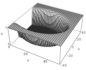
Figure 4: The scalar field $\phi$ in the $rz$-plane for $N_{CS}=12^{\prime}000$ and $\beta=1$. Note that $\phi$ is shown in units of $v$ and the coordinates $r$ and $z$ are in units of $1/m_{V}$. The rectangular box in the $rz$-plane used to obtain the solution in this case was $[0,52]\times[-40,40]$.

Figure 5: The scalar field $\phi$ along the axis of symmetry $r=0$ (again for $N_{CS}=12^{\prime}000$ and $\beta=1$). The dots show the values of $\phi$ on the grid points of the numerical solution. The resolution is $0.8/m_{V}$.

show a 3D-plot of the scalar field $\phi$ in the $rz$-plane and a 2D-plot of $\phi$ along the axis of symmetry $r=0$, respectively. The thickness of the domain wall ($\sim 1/m_{H}$), which separates the two phases $\phi\ll v$ and $\phi=v$, is small compared to the size of the soliton (thin wall approximation).

Moreover Fig. 4 shows that the soliton is not spherically symmetric. We can determine the shape of the soliton numerically. For this end, we define the contour of constant scalar field $\phi=0.5\ v$ as the boundary of the soliton and fit a 2-dimensional surface to that boundary. This is done in Fig. 6,

Figure 6: The dotted line shows the contour of constant scalar field $\phi=0.5$ in the $rz$-plane. The solid line is the best fitting circle to the dotted line, which is the circle around ($18.163,0$) with radius $r_{s}\approx 27.132$ (in units of $1/m_{V}$).

in which we show the contour $\phi=0.5\ v$ in the $rz$-plane. The contour follows very precisely a circle of radius $r_{s}\approx 27.132/m_{V}$ centered at $(18.163/m_{V},0)$. The contour deviates from a perfect circle just in a narrow region around the axis of symmetry, whose size is of the order of a few $1/m_{V}$. Only in this small region, the fields behave microscopically. Motivated by the amazing numerical result of Fig. 6, we conjecture that asymptotically for large $N_{CS}$, the soliton has the shape of a so-called spindle torus. A spindle torus is the surface of revolution obtained by rotating a circular arc around an axis, where the arc is intersecting that axis. However, we were not able to prove this result analytically.

We now turn to the gauge field. As depicted in Fig. 7,

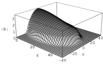
Figure 7: 3D-plot of the magnetic field $|\bm{B}|$ in the $rz$-plane in units of the critical magnetic field $B_{c}$.

the magnetic field is confined to the region where the scalar field is vanishing or small. Inside this domain the amplitude of the magnetic field $|\bm{B}|$ is larger than the critical magnetic field $B_{c}$.

On the boundary $|\bm{B}|=B_{c}$ and $\bm{B}$ is tangential to the domain boundary (see Fig. 8).

Figure 8: The dots show the tangential component $\bm{B}_{\parallel}$ of the magnetic field along the boundary of the domain as a function of the distance $r$ from the axis of symmetry (units for $\bm{B}_{\parallel}$: $B_{c}=1$). Sufficiently far away from the axis of symmetry the magnetic field is constant and equal to the critical field $B_{c}$, which is represented by the solid line.

Remember that this behavior is expected from (type I) superconductors in the intermediate state: on the boundaries of normal-conducting regions the magnetic field is tangential and equal to $B_{c}$. Outside this boundary, where the scalar field starts to deviate from zero, the magnetic field decays exponentially, because in the broken phase the gauge boson becomes massive.

To get an idea of how the magnetic field lines behave, we show in Fig. 9 a

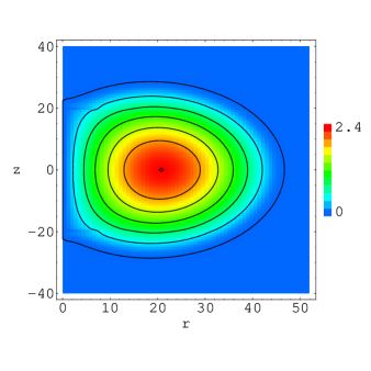
Figure 9: Contour plot of the toroidal component $B_{\varphi}$ of the magnetic field (in units of the critical magnetic field $B_{c}$). The shown contours are from $0$ to $2.4$ with a step size of $0.4$ between the contours. The maximal value of $B_{\varphi}$ is located at $(r,z)\approx(20.8,0)$ and is equal to $2.4\ B_{c}$.

plot of the “toroidal” component $B_{\varphi}$ and in Fig. 10 the

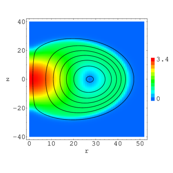
Figure 10: The poloidal component $\bm{B}_{p}$ of the magnetic field. The solid lines are projections of the field lines onto the $rz$-plane. The colors indicate the modulus of $\bm{B}_{p}$ (in units of $B_{c}$). The poloidal field is maximal at the origin and vanishes at $(27.4,0)$. On the boundary of the spindle torus $|\bm{B}_{p}|=B_{c}$.

“poloidal” component $\bm{B}_{p}=(B_{r},B_{z})$ of the magnetic field. The toroidal component of the magnetic field is maximal at $(20.8/m_{V},0)$ and vanishes on the boundary of the spindle torus, where the field is completely poloidal. The poloidal field is maximal at the origin and zero at $(27.4/m_{V},0)$. As it was already shown in Fig. 8, $|\bm{B}_{p}|=B_{c}$ along the boundary of the spindle torus. In short terms, the poloidal component of the magnetic field wraps around the toroidal component, giving rise to the non-zero helicity of the magnetic field (which is the same as Chern-Simons number for Abelian fields).

Finally we show in Fig. 11

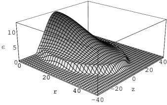
Figure 11: 3D plot of the energy density for the soliton with $N_{CS}=12^{\prime}000$ and $\beta=1$ (in units of the vacuum energy density $\lambda v^{4}$). The maximum of the energy density is at the origin and is equal to $\mathcal{E}_{max}\approx 12.56\ \lambda v^{4}=6.28\ B_{c}^{2}$.

the energy density of the soliton ($N_{CS}=12^{\prime}000$ and $\beta=1$). The different parts of the energy are

$$E_{\text{magn}} = \int\frac{\bm{B}^{2}}{2}\ d^{3}x\approx 1.00158\cdot 10^{5}\ m_{V}/g^{2}\ ,$$ (47)

$$E_{\text{D}} = \int\left[(\bm{\nabla}\phi)^{2}+g^{2}\bm{A}^{2}\phi^{2}\right]\ d^{3}x\approx 3.985\cdot 10^{3}\ m_{V}/g^{2}\ ,$$ (48)

$$E_{\text{V}} = \int\lambda(\phi^{2}-v^{2})^{2}\ d^{3}x\approx 3.2123\cdot 10^{4}\ m_{V}/g^{2}\ .$$ (49)

The virial theorem (30) is very well satisfied ($E_{\text{magn}}=3E_{\text{V}}+E_{\text{D}}$ to an accuracy of less than $1\%$). The part $E_{\text{D}}$ of the energy is a surface term and is negligible for sufficiently large Chern-Simons number.

IV.4 Solitons for different scalar potentials

In section III.4, we have seen that for a scalar potential like the one shown in Fig. 1, the energy of anomalous solitons is $E\sim N_{CS}^{2/3}$.

In order to verify this conjecture, we also solved the field equations for the potential

$$V(\phi)=\gamma(\phi-v)^{2}\phi^{2}\ .$$ (50)

If we again use dimensionless fields and coordinates as before, the field equations (42) for the potential (50) read

$$\bm{\nabla}^{2}\phi-\frac{1}{2}\bm{A}^{2}\phi-\frac{\widetilde{\beta}}{4}\left[\phi\left(\phi-1\right)^{2}+\phi^{2}\left(\phi-1\right)\right] =0\ ,$$ (51a)

$$\bm{\nabla}\times\left(\bm{\nabla}\times\bm{A}\right)-2\mu\bm{\nabla}\times\bm{A}+\phi^{2}\bm{A} =0\ ,$$ (51b)

with $\widetilde{\beta}=2\gamma/g^{2}$. The constraint equation (43) remains unchanged. We solved Eqs. (51) for $10<N_{CS}<700$ and $\widetilde{\beta}=1$. In Fig. 12

Figure 12: Logarithmic plot of the energy as a function of $N_{CS}$ for anomalous solitons obtained with the potential (50). The dots show the values of our numerical solutions and the solid line is the best fit of the form $E=aN_{CS}^{2/3}$, which gives $a\approx 94.866\ m_{V}/g^{2}$.

we show the energy of the obtained solutions as a function of $N_{CS}$. We find

$$E\approx 94.866\ m_{V}/g^{2}\ N_{CS}^{2/3}\ ,$$ (52)

which confirms the claim of section III.4. Fig. 13

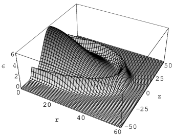
Figure 13: The energy density of the soliton with $N_{CS}=500$ and $\widetilde{\beta}=1$ in units of $\gamma v^{4}/16$ (which is the potential barrier between the two minima of the potential).

shows the energy density the soliton with $N_{CS}=500$ and $\tilde{\beta}=1$. The main contribution still comes from the magnetic field, but one can clearly see that there is a contribution located on the surface, which is the energy of the scalar field. As well in this case, the solitons are not spherical.

V Thin Wall Approximation

In this section we construct the anomalous solitons in the thin wall approximation valid for large $N_{CS}$. In this limit the solitons are described by a compact domain $V$, inside which $\phi=0$. Outside the domain we have $\phi=v$ and $\bm{A}=0$. In order to determine $\bm{A}$ inside $V$ we have to solve Eq. (11b) for $\phi=0$,

$$\bm{\nabla}\times\left(\bm{\nabla}\times\bm{A}\right)=2\mu\left(\bm{\nabla}\times\bm{A}\right)\ ,$$ (53)

where $\bm{A}=0$ on the boundary $\partial V$. In principle, the surface $\partial V$ has also to be determined by minimization. But because we have found numerically in the previous section, that the solitons have the shape of a spindle torus for large $N_{CS}$, we take $\partial V$ to be a spindle torus of fixed size described by two parameters $R_{s}$ and $r_{s}>R_{s}$ (see Fig. 14).

Figure 14: Cross-section of a spindle torus in the $rz$-plane with radii $R_{s}$ and $r_{s}$. The spindle torus is obtained by rotating the circle centered at $(R_{s},0)$ with radius $r_{s}>R_{s}$ around the $z$ axis.

We solve Eq. (53) inside the spindle torus as a function of $R_{s}$ and $r_{s}$. Then we minimize the soliton energy with respect to these two parameters. We use dimensionless cylindrical coordinates $(\varrho,\varphi,\zeta)$ defined by

$$x = R_{s}\varrho\cos\varphi\ ,$$

$$y = R_{s}\varrho\sin\varphi\ ,$$

$$z = R_{s}\zeta\ .$$

In these coordinates (53) simplifies to a system of linear partial differential equations for the potentials $A_{\varrho}$, $A_{\varphi}$ and $A_{\zeta}$ in the $\varrho\zeta$-plane

$$\partial_{\zeta}\left(\partial_{\zeta}A_{\varrho}-\partial_{\varrho}A_{\zeta}\right) = \nu\ \partial_{\zeta}A_{\varphi}\ ,$$ (54a)

$$-\partial_{\zeta}^{2}A_{\varphi}-\partial_{\varrho}\left[\frac{1}{\varrho}\partial_{\varrho}\left(\varrho A_{\varphi}\right)\right] = \nu\ \left(\partial_{\zeta}A_{\varrho}-\partial_{\varrho}A_{\zeta}\right)\ ,$$ (54b)

$$\frac{1}{\varrho}\partial_{\varrho}\left[\varrho\left(\partial_{\zeta}A_{\varrho}-\partial_{\varrho}A_{\zeta}\right)\right] = \nu\ \frac{1}{\varrho}\partial_{\varrho}\left(\varrho A_{\varphi}\right)\ ,$$ (54c)

with $\nu=2\mu R_{s}$.
Integration of (54a) and (54c) gives

$$\nu A_{\varphi}=\partial_{\zeta}A_{\varrho}-\partial_{\varrho}A_{\zeta}=R_{s}B_{\varphi}$$ (55)

and using (55) in (54b) leads to

$$\partial_{\varrho}\left[\frac{1}{\varrho}\partial_{\varrho}\left(\varrho A_{\varphi}\right)\right]+\partial_{\zeta}^{2}A_{\varphi}+\nu^{2}A_{\varphi}=0\ .$$ (56)

The Chern-Simons number becomes

$$N_{CS} = \frac{g^{2}}{16\pi^{2}}\int\bm{A}\cdot\bm{B}\ d^{3}x$$ (57)

$$= \frac{g^{2}}{8\pi^{2}}\int A_{\varphi}B_{\varphi}\ d^{3}x$$

$$= \frac{g^{2}\nu}{8\pi^{2}R_{s}}\int A_{\varphi}^{2}\ d^{3}x\ ,$$

where the second line is found by partial integration and Eq. (55) has been used on the third line. We solved Eq. (56) numerically with $A_{\varphi}=0$ on the boundary of the spindle torus and under the constraint (57). Because Eq. (56) is a linear eigenvalue problem, the solution which minimizes the energy is the eigenfunction to the lowest positive eigenvalue $\nu^{2}$, normalized with Eq. (57). It turns out, that the eigenvalue $\nu$ is a function of the ratio $\varrho_{s}=r_{s}/R_{s}$, which is shown in Fig. 15. The total

Figure 15: The eigenvalue $\nu$ as a function of the parameter $\varrho_{s}$.

energy of the solution is given by Eq. (15) for $R=R_{s}$. After minimization with respect to $R_{s}$, the size of the spindle torus $R_{s}$ and the energy are given by (cf. Eqs. (16) and (17))

$$R_{s}(\varrho_{s}) = \left[\frac{64\pi^{2}\nu(\varrho_{s})}{3I_{V}(\varrho_{s})}\right]^{1/4}\frac{1}{m_{V}}\left(\frac{N_{CS}}{\beta}\right)^{1/4}\ ,$$ (58)

$$E(\varrho_{s}) = \sqrt{2}\left[\frac{16\pi^{2}\nu(\varrho_{s})}{3}\right]^{3/4}\left[I_{V}(\varrho_{s})\beta\right]^{1/4}\frac{m_{V}}{g^{2}}N_{CS}^{3/4}\ ,$$ (59)

where the shape factor for the spindle torus is

$$I_{V}(\varrho_{s})=\pi^{2}\varrho_{s}^{2}+2\pi\sqrt{\varrho_{s}^{2}-1}+\frac{4\pi}{3}\left(\varrho_{s}^{2}-1\right)^{3/2}+2\pi\varrho_{s}^{2}\arcsin\left(\frac{1}{\varrho_{s}}\right)\ .$$ (60)

In Fig. 16 we show the function $E(\varrho_{s})$,

Figure 16: The total energy $E$ as a function of the parameter $\varrho_{s}$. The minimal energy is at $\varrho_{s}\approx 1.495$ and is $E_{\text{min}}\approx 119.06\ \beta^{1/4}(m_{V}/g^{2})N_{CS}^{3/4}$.

which can be minimized numerically with respect to $\varrho_{s}$. There is a minimum at $\varrho_{s}\approx 1.495$, for which we get

$$R_{s} \approx 1.742\ \frac{1}{m_{V}}\left(\frac{N_{CS}}{\beta}\right)^{1/4}\ ,$$ (61)

$$E \approx 119.065\ \beta^{1/4}\frac{m_{V}}{g^{2}}N_{CS}^{3/4}\ .$$ (62)

These results are in excellent agreement with the results of the previous section, where we obtained

$$R_{s} \approx 1.726\ \frac{1}{m_{V}}\left(\frac{N_{CS}}{\beta}\right)^{1/4}\ ,$$ (63)

$$E \approx 118.826\ \beta^{1/4}\frac{m_{V}}{g^{2}}N_{CS}^{3/4}\ .$$ (64)

The macroscopic solutions discussed in the present section coincide with the solutions of the previous section for large $N_{CS}$. To illustrate this, we compare in Fig. 17 the

Figure 17: The amplitude of the magnetic field $|\bm{B}|$ in the plane $z=0$ of the soliton with $N_{CS}=12^{\prime}000$ and $\beta=1$. The dotted line shows the solution of the previous section, the solid line is the solution in the thin wall (macroscopic) approximation discussed in the present section. The units are $B_{c}=1$.

magnetic fields of the macroscopic solution and the solution of the previous section.

VI Conclusions

In this article we studied anomalous Abelian solitons, a class of solitons of the chiral Abelian Higgs model found by Rubakov and Tavkhelidze. These solitons carry a non-zero Chern-Simons number $N_{CS}$ and they are stable for large $N_{CS}$. We showed that their energy-versus-fermion-number ratio is given by $E\sim N_{CS}^{3/4}$ or $E\sim N_{CS}^{2/3}$ depending on the structure of the scalar potential. For the former case we derived a lower bound for the soliton energy, $E\geq cN_{CS}^{3/4}$, where $c$ is a constant depending on the coupling constants and the VEV of the Higgs field.

We discussed the structure of anomalous solitons by solving numerically the field equations for both the gauge and the Higgs field. It turned out that the solitons are not spherically symmetric. For large Chern-Simons number they have the shape of a spindle torus. In this limit we also constructed the solutions in the thin wall (macroscopic) approximation.

At the moment it is not clear, if (metastable) anomalous solitons exist in the standard model. It will be interesting to extend the present study to the full electroweak theory with $SU(2)\times U(1)$ gauge group.

Appendix A Inequalities

In this appendix we review the inequalities from functional analysis, which have been used in Sec. III.1 to derive the lower bound on the energy of the anomalous solitons.

A.1 Hölder inequality

Let $\Omega$ be an open subset of $\mathbb{R}^{d}$ and $p,\ q\geq 1$ such that

$$\frac{1}{p}+\frac{1}{q}=1\ .$$

Then, for all functions $f\in L^{p}(\Omega)$ and $g\in L^{q}(\Omega)$, the product $fg\in L^{1}(\Omega)$ satisfies the Hölder inequality,

$$\lVert fg\rVert_{L^{1}}\leq\lVert f\rVert_{L^{p}}\lVert g\rVert_{L^{q}}\ ,$$ (65)

where the norm on $L^{p}(\Omega)$ is defined by

$$\lVert f\rVert_{L^{p}}:=\left(\int\limits_{\Omega}\lvert f\rvert^{p}\ dx\right)^{1/p}\ .$$

Note that for $p=q=2$ the Hölder inequality reduces to the Cauchy-Schwarz inequality. For vector fields $\bm{u}(\bm{x}):\Omega\rightarrow\mathbb{R}^{d}$ the $L^{p}$-norm is defined by

$$\lVert\bm{u}\rVert_{L^{p}}=\left(\int\limits_{\Omega}(\bm{u},\bm{u})^{p/2}\ dx\right)^{1/p}\ ,$$

where $(\cdot,\cdot)$ denotes the scalar product of vectors in $\mathbb{R}^{d}$. Thus for vector fields the Hölder inequality reads

$$\Biggl{|}\int\limits_{\Omega}(\bm{u},\bm{v})\ dx\Biggr{|}\leq\lVert\bm{u}\rVert_{L^{p}}\lVert\bm{v}\rVert_{L^{q}}\ .$$ (66)

A.2 “Modified” Hölder inequality

As a consequence of (65) we have for $s>1$ that

$$\lVert f\rVert_{L^{s}}^{s}\leq\lVert f\rVert_{L^{1}}^{2-s}\lVert f\rVert_{L^{2}}^{2s-2}\ ,\quad\forall f\in L^{s}(\Omega)\ .$$ (67)

The proof of (67) is very simple: defining the functions $g$ and $h$ by

$$g =|f|^{2-s}\ ,$$

$$h =|f|^{2s-2}\ ,$$

we get

$$\lVert f\rVert_{L^{s}}^{s} =\lVert gh\rVert_{L^{1}}$$

$$\leq\lVert g\rVert_{L^{1/(2-s)}}\lVert h\rVert_{L^{1/(s-1)}}$$

$$=\left(\int\limits_{\Omega}|g|^{1/(2-s)}\ dx\right)^{2-s}\left(\int\limits_{\Omega}|h|^{1/(s-1)}\ dx\right)^{s-1}$$

$$=\left(\int\limits_{\Omega}|f|\ dx\right)^{2-s}\left(\int\limits_{\Omega}|f|^{2}\ dx\right)^{\frac{2s-2}{2}}$$

$$=\lVert f\rVert_{L^{1}}^{2-s}\lVert f\rVert_{L^{2}}^{2s-2}\ ,$$

where (65) has been used on the second line.

A.3 Gagliardo-Nirenberg-Sobolev inequality

The Sobolev spaces $W^{n,p}(\Omega)$, where $p\geq 1$ and $n\in\mathbb{N}$, are the normed spaces of functions defined by

$$W^{n,p}(\Omega)=\Bigl{\{}f\in L^{p}(\Omega)\big{|}\ \forall\alpha\in\mathbb{N}^{d},\ |\alpha|\leq n:\partial^{\alpha}_{x}f\in L^{p}(\Omega)\Bigr{\}}\ .$$

For $1\leq p<d$ we define the Sobolev conjugate of $p$ by

$$p^{*}=\frac{dp}{d-p}\ .$$

Then, there is a constant $c(d,p)$, such that

$$\lVert f\rVert_{L^{p^{*}}}\leq c(d,p)\ \lVert Df\rVert_{L^{p}}\ ,\quad\forall f\in W^{1,p}(\Omega)\ ,$$ (68)

where $D$ is the weak derivative. (68) is known as Gagliardo-Nirenberg-Sobolev (GNS) inequality. For $\Omega=\mathbb{R}^{d}$ the best possible constant in (68) is

$$c(d,p)=\begin{cases}\frac{1}{d}\left(\frac{d}{|S^{d-1}|}\right)^{1/d}&p=1\\ \frac{p-1}{d-p}\left[\frac{d-p}{d(p-1)}\right]^{1/p}\left[\frac{\Gamma(d+1)}{\Gamma\left(d/p\right)\Gamma\left(d+1-d/p\right)|S^{d-1}|}\right]^{1/d}&p>1\ .\end{cases}$$

Here, $|S^{d-1}|$ denotes the surface area of the $(d-1)$-dimensional unit sphere,

$$|S^{d}|=2^{d}\pi^{d/2}\frac{\Gamma(d/2)}{\Gamma(d)}\ .$$

In Sec. III.1 we have used (68) for continuosly differentiable functions with compact support and $(d,p)=(3,2)$. In this case the weak derivative is just the ordinary gradient and the GNS inequality reads

$$\lVert f\rVert_{L^{6}}\leq c(3,2)\ \lVert\bm{\nabla}f\rVert_{L^{2}}=\frac{1}{\sqrt{3}}\left(\frac{2}{\pi}\right)^{2/3}\ \lVert\bm{\nabla}f\rVert_{L^{2}}\ ,\quad\forall f\in C^{1}_{c}(\mathbb{R}^{3})\ .$$ (69)

Appendix B Numerical procedure

In this appendix we explain the numerical procedure which was used to obtain numerical solutions of the PDEs (44) subject to the constraint (45) and boundary conditions (46). Solutions are calculated on the rectangular box $[0,L]\times[-Z,Z]$ in the $rz$-plane. The dimensions of the box $L$ and $Z$ have to be at least a few times $N_{CS}^{1/4}$, since the expected size of the soliton is $R\sim N_{CS}^{1/4}$. The box is divided into a grid of $N_{r}\times N_{z}$ points $(r_{i},z_{i})$ given by

$$r_{i} =h_{r}(i-1)\ ,\qquad\qquad\text{for}\quad i=1,\ldots,N_{r}\ ,$$

$$z_{j} =\frac{h_{z}}{2}(2j-1-N_{z})\ ,\quad\text{for}\quad j=1,\ldots,N_{z}\ ,$$

where $h_{r}=L/(N_{r}-1)$ and $h_{z}=2Z/(N_{z}-1)$. Because the coordinates $(r,z)$ are in units of $1/m_{V}$ and we expect the fields to vary on scales of order $1/m_{H}$ and $1/m_{V}$, $h_{r}$ and $h_{z}$ have to be smaller than $\beta^{1/2}$ to ensure a sufficient resolution of the solutions. Therefore, the number of grid points has to be increased going either to larger $N_{CS}$ or to lower $\beta$. As an example for $N_{CS}=12^{\prime}000$ and $\beta=1$, we were using the rectangular box $[0,52]\times[-40,40]$ with a resolution of $0.8/m_{V}$, which lead to a grid with $6^{\prime}666$ points.

The derivatives in the PDEs (44) are approximated by finite differences in a straightforward way,

$$f(r_{i},z_{j}) \rightarrow f_{i,j}\ ,$$

$$(\partial_{r}f)(r_{i},z_{j}) \rightarrow\frac{1}{2h_{r}}\left(f_{i+1,j}-f_{i-1,j}\right)\ ,$$

$$(\partial_{z}f)(r_{i},z_{j}) \rightarrow\frac{1}{2h_{z}}\left(f_{i,j+1}-f_{i,j-1}\right)\ ,$$

$$(\partial_{r}^{2}f)(r_{i},z_{j}) \rightarrow\frac{1}{h_{r}^{2}}\left(f_{i+1,j}-2f_{i,j}+f_{i-1,j}\right)\ ,$$

$$(\partial_{r}\partial_{z}f)(r_{i},z_{j}) \rightarrow\frac{1}{4h_{r}h_{z}}\left(f_{i+1,j+1}-f_{i+1,j-1}-f_{i-1,j+1}+f_{i-1,j-1}\right)\ ,$$

$$(\partial_{z}^{2}f)(r_{i},z_{j}) \rightarrow\frac{1}{h_{z}^{2}}\left(f_{i,j+1}-2f_{i,j}+f_{i,j-1}\right)\ ,$$

where $f(r_{i},z_{j})$ stands for one of the fields $A_{r}$, $A_{\varphi}$, $A_{z}$ or $\phi$ at the position $(i,j)$ on the grid. Using these replacement rules the PDEs reduce to a system of non-linear equations on the internal points of the grid (i.e. $i=2,\ldots,N_{r}-1$ and $j=2,\ldots,N_{z}-1$). On the axis of symmetry $r=0$ the finite difference approximation for the PDEs requires special care. The regularity conditions (46c) at $r=0$ for the fields $A_{r}$ and $A_{\varphi}$ imply

$$A_{r,1,j} =0\ ,$$ (70)

$$A_{\varphi,1,j} =0\ ,$$ (71)

for $j=2,\ldots,N_{z}-1$. For discretizing Eqs. (44a) and (44d) at $r=0$ we have to use the replacements

$$\frac{1}{r}\partial_{r}\left(r\partial_{r}\phi\right)_{r=0}=2\partial_{r}^{2}\phi\Big{|}_{r=0} \rightarrow\frac{4}{h_{r}^{2}}\left(\phi_{2,j}-\phi_{1,j}\right)\ ,$$

$$\frac{1}{r}\partial_{r}\left(r\partial_{r}A_{z}\right)_{r=0}=2\partial_{r}^{2}A_{z}\Big{|}_{r=0} \rightarrow\frac{4}{h_{r}^{2}}\left(A_{z,2,j}-A_{z,1,j}\right)\ ,$$

$$\frac{1}{r}\partial_{r}\left(r\partial_{z}A_{r}\right)_{r=0}=2\partial_{r}\partial_{z}A_{r}\Big{|}_{r=0} \rightarrow\frac{1}{h_{r}h_{z}}\left(A_{r,2,j+1}-A_{r,2,j-1}\right)\ ,$$

$$\frac{1}{r}\partial_{r}\left(rA_{\varphi}\right)_{r=0}=2\partial_{r}A_{\varphi}\Big{|}_{r=0} \rightarrow\frac{2}{h_{r}}A_{\varphi,2,j}\ .$$

The system of non-linear equations is completed by the boundary conditions at $r=L$ and $z=\pm Z$, which read

$$\phi_{i,1} =\phi_{i,N_{z}}=1\quad\text{and}\quad\bm{A}_{i,1}=\bm{A}_{i,N_{z}}=0\quad\text{for}\quad i=1,\ldots,N_{r}\ ,$$ (72a)

$$\phi_{N_{r},j} =1\qquad\qquad\text{and}\qquad\bm{A}_{N_{r},j}=0\qquad\text{for}\quad j=1,\ldots,N_{z}\ .$$ (72b)

Finally, the constraint equation (45) is given by

$$N_{CS}=\frac{h_{r}h_{z}}{8\pi}\sum_{i=2}^{N_{r}-1}\sum_{j=2}^{N_{z}-1}h_{r}(i-1)A_{\varphi,i,j}\left(\frac{A_{r,i,j+1}-A_{r,i,j-1}}{2h_{z}}-\frac{A_{z,i+1,j}-A_{z,i-1,j}}{2h_{r}}\right)\ .$$ (73)

Including the constraint equation (73) we obtain a system of $4N_{r}N_{z}+1$ non-linear equations for the unkowns $\phi_{i,j}$, $A_{r,i,j}$, $A_{\varphi,i,j}$, $A_{z,i,j}$ and the Lagrangian multiplier $\mu$. This system is solved using a standard Newtonian algorithm for non-linear equations. In every step of the Newton iteration, one has to solve a system of $4N_{r}N_{z}+1$ linear equations.

References

- (1) D. Finkelstein and C.W. Misner, Annals Phys. 6 (1959) 230.
- (2) D. Finkelstein, J. Math. Phys. 7 (1966) 1218.
- (3) A.A. Abrikosov, Sov. Phys. JETP 5 (1957) 1174.
- (4) H.B. Nielsen and P. Olesen, Nucl. Phys. B61 (1973) 45.
- (5) A.M. Polyakov, JETP Lett. 20 (1974) 194.
- (6) G. ’t Hooft, Nucl. Phys. B79 (1974) 276.
- (7) T.H.R. Skyrme, Nucl. Phys. 31 (1962) 556.
- (8) R. Friedberg, T.D. Lee and A. Sirlin, Phys. Rev. D13 (1976) 2739.
- (9) S.R. Coleman, Nucl. Phys. B262 (1985) 263.
- (10) A.M. Safian, S.R. Coleman and M. Axenides, Nucl. Phys. B297 (1988) 498.
- (11) S.Y. Khlebnikov and M.E. Shaposhnikov, Phys. Lett. B180 (1986) 93.
- (12) E.J. Copeland, E.W. Kolb and K.M. Lee, Nucl. Phys. B319 (1989) 501.
- (13) V.A. Rubakov and A.N. Tavkhelidze, Phys. Lett. B165 (1985) 109.
- (14) L.D. Faddeev and A.J. Niemi, Nature 387 (1997) 58, hep-th/9610193.
- (15) V.A. Rubakov, Prog. Theor. Phys. 75 (1986) 366.
- (16) V.A. Matveev et al., Nucl. Phys. B282 (1987) 700.
- (17) G. ’t Hooft, Phys. Rev. Lett. 37 (1976) 8.
- (18) R. Jackiw and C. Rebbi, Phys. Rev. Lett. 37 (1976) 172.
- (19) C.G. Callan Jr, R.F. Dashen and D.J. Gross, Phys. Lett. B63 (1976) 334.
- (20) A.N. Redlich and L.C.R. Wijewardhana, Phys. Rev. Lett. 54 (1985) 970.
- (21) A.F. Vakulenko and L.V. Kapitansky, Sov. Phys. Dokl. 24 (1979) 433.
- (22) A. Kundu and Y.P. Rybakov, J. Phys. A15 (1982) 269.
- (23) R.S. Ward, Nonlinearity 12 (1999) 241, hep-th/9811176.
- (24) G. Rosen, SIAM Journal on Applied Mathematics 21 (1971) 30.
- (25) L.D. Landau and L.P. Pitaevskii, Statistical Physics: Part 2, second ed. (Pergamon Press, Oxford, 1981).
- (26) L.D. Landau and E.M. Lifshitz, Electrodynamics of Continuous Media, first ed. (Pergamon Press, Oxford, 1960).