Casimir effect in rugby-ball type flux compactifications

Abstract

As a continuation of the work in mns , we discuss the Casimir effect for a massless bulk scalar field in a 4D toy model of a 6D warped flux compactification model, to stabilize the volume modulus. The one-loop effective potential for the volume modulus has a form similar to the Coleman-Weinberg potential. The stability of the volume modulus against quantum corrections is related to an appropriate heat kernel coefficient. However, to make any physical predictions after volume stabilization, knowledge of the derivative of the zeta function, $\zeta^{\prime}(0)$ (in a conformally related spacetime) is also required. By adding up the exact mass spectrum using zeta function regularization, we present a revised analysis of the effective potential. Finally, we discuss some physical implications, especially concerning the degree of the hierarchy between the fundamental energy scales on the branes. For a larger degree of warping our new results are very similar to the ones given in Ref mns and imply a larger hierarchy. In the non-warped (rugby-ball) limit the ratio tends to converge to the same value, independently of the bulk dilaton coupling.

I Introduction

Recent studies on braneworld models with extra dimensions that are compactified by a magnetic flux and bounded by codimension 2 branes (conical singularities) Sidestep ; Gibbons:2003di have revealed various fundamental properties, i.e., the regularization of branes (conical singularities)/linearized gravity deRham:2005ci ; Peloso:2006cq ; Carter:2006uk and stability against classical perturbations SusyPerts ; nonSUSYpert . There are still a lot of unsolved questions which should be clarified, especially concerning non-linear gravity and cosmology. Furthermore, careful analysis of these simpler models may give important physical insights on self-gravitating branes in various flux compactifications in string theory Douglas:2006es .

In this paper, we focus on models of braneworld based on a 6D supergravity Gibbons:2003di , though we will work with its 4D counterpart 4D , because of the lack of a formulation of the heat kernel coefficients for conical singularities in 6D. In these supergravity inspired models, the size of the compactified internal-space is not fixed classically and may behave as a volume modulus in a 4D effective theory. To fix this size of the volume (the volume modulus), we should therefore discuss other additional mechanisms. The authors of Ref. mns focused on Casimir corrections for the case of perturbations of a massless, minimally coupled bulk scalar field. In this article, we present a revised analysis of the previous calculations, by performing a strict mode summation of the exact mass spectrum, which is now wholly taken into account.

We give an exact analysis of the one-loop effective action in a 4D alternative model. The one-loop effective potential for the volume modulus can be written in a form which is somewhat similar to the Coleman-Weinberg potential:

$$V_{\rm 4,eff}=\frac{A_{4}-B_{4}\ln(\mu^{2}\rho_{+})}{\rho_{+}}\,,$$ (1)

where $\rho_{+}$ characterizes the volume modulus and $A_{4}$ and $B_{4}$ are functions of the model parameters and the shape modulus (the degree of the warping of the bulk, which is completely determined if one fixes the brane tensions). Stability itself is determined by the sign of $B_{4}$, which is closely related to the relevant heat kernel coefficients. However, to discern phenomenological effects on the brane, i.e., the effective mass of the modulus and the degree of the hierarchy between fundamental energy scales on the brane, we need to know the value of $A_{4}$ as well. $A_{4}$ is not just related to the heat kernel, although partly related with it; we also need to evaluate $\zeta^{\prime}(0)$. Thus, an accurate evaluation of $A_{4}$ is crucial to make physical predictions, e.g., for the hierarchy or cosmological constant (CC) problems.

In the work mns , it has been shown how to divide $A_{4}$ into two parts, by introducing a continuous conformal transformation, going from the unwarped frame to the original warped geometry. The first part is associated with a one parameter family of conformal transformations and is called the cocycle function. This term can be obtained from heat kernel analysis. The second part consists of calculating the derivative of the zeta function in the unwarped frame, where to evaluate this piece we used the WKB approximation. In this paper we shall present an exact analysis of the mass spectrum for these Kaluza-Klein like modes in the unwarped frame.

The structure of the article is as follows: In the next section we briefly discuss our 4D analogue warped flux compactification model and review the tools to analyze the one-loop Casimir effect. We give the exact mass spectrum in the unwarped rugby-ball frame. In Sec. III we carry out the zeta function regularization in the unwarped frame. In Sec. IV, we give physical implications of our result, e.g., for the hierarchy problem by making comparisons with the results in mns . We finish this article after giving a summary and some discussions.

II 4D warped flux compactification model

Our main interest is the Casimir effect in the warped flux compactification model in 6D supergravity Gibbons:2003di :

$$S_{6}=M_{6}^{4}\int d^{6}x\sqrt{-g}\left(\frac{1}{2}R-\frac{1}{2}\partial_{A}\varphi\partial^{A}\varphi-\frac{1}{4}e^{-\varphi}F_{AB}F^{AB}-2g_{0}^{2}e^{\varphi}\right)\,,$$ (2)

where $F_{AB}$ is the field strength of the electromagnetic field, $\varphi$ is the dilaton, and $g_{0}$ is the bulk dilaton coupling. Hereafter, we set $M_{6}^{4}=1$ and if needed, we put it back explicitly. In order to evaluate the Casimir energy in this model, we need to know the heat kernel coefficients on the conical singularities. However, as mentioned in mns , there is no mathematical formulation of these coefficients the authors are aware of. Thus, in this paper, we focus on its 4D counterpart theory:

$$S_{4}=M_{4}^{2}\int d^{4}x\sqrt{-g}\left(R-\frac{1}{2}\partial_{A}\varphi\partial^{A}\varphi-\frac{1}{8}e^{-\varphi}F_{AB}F^{AB}-4g^{2}e^{\varphi}\right)\,,$$ (3)

which has a series of warped flux compactification solutions 4D

$$ds^{2} = h(\rho)d\theta^{2}+\frac{d\rho^{2}}{h(\rho)}+(2\rho)(-d\tau^{2}+dx_{2}^{2})\,,\quad h(\rho)=\frac{2g^{2}}{\rho}\left(\rho_{+}-\rho\right)\left(\rho-\rho_{-}\right)\,,$$ (4)

$$\varphi(\rho)=-\ln(2\rho)\,,\quad F_{\theta\rho}=-\frac{Q}{\rho^{2}}\,.$$

We also set $M_{4}=1$ unless it is needed. Then, the branes correspond to strings, lying at the positions given by the horizon-like condition $h(\rho)=0$. It is useful to define the coordinate $z=((\rho_{+}-\rho)/(\rho-\rho_{-}))^{1/2}$, to resolve the structure of spacetime in the case that $\rho_{+}=\rho_{-}$. For $z\to 0,\infty$, there are cones whose deficit angles are obtained from the relation $\delta_{\pm}:=2\pi-g^{2}(\rho_{+}-\rho_{-})\Delta\theta/(\rho_{\pm})$.

The moduli in the effective theory on the branes are characterized by $\rho_{\pm}$, or equivalently by $\rho_{+}$ and $r$, where the string tensions are related to the conical deficits by $\sigma_{\pm}=M_{4}^{2}\delta_{\pm}$. We stress that these relations are only valid for sufficiently small brane tensions, in comparison with the bulk scale $M_{4}^{2}$. The coordinate $\theta$ is defined as $0\leq\theta<\Delta\theta$ and $\Delta\theta$ is given by

$$\Delta\theta(r,\delta_{+})=\frac{2\pi-\delta_{+}}{g^{2}(1-r)}\,,$$ (5)

where $r:=\rho_{-}/\rho_{+}$. Once the brane tensions, $\sigma_{+}$ and $\sigma_{-}$ are fixed, then $r$ is also fixed and so we now regard as free parameters $r$ and $\delta_{+}$, along with the dilaton bulk coupling $g$. The remaining degree of freedom used to determine the bulk geometry is the absolute size of the bulk, i.e., $\rho_{+}$, which should be fixed by additional mechanisms.

We discuss the basic properties of a massless, minimally coupled scalar field on this background:

$$S_{\rm scalar}=-\frac{1}{2}\int d^{4}x\sqrt{g}\phi\Delta_{4}\phi\,.$$ (6)

Now consider a continuous conformal transformation of the metric, parameterized by $\epsilon$;

$$d{\tilde{s}}_{4,\epsilon}^{2}=e^{2(\epsilon-1)\omega}ds_{4}^{2}\,,\qquad\omega=\frac{1}{2}\ln(2\rho)\,,$$ (7)

where for $\epsilon=1$ we have the original metric, which we shall define as $\Delta_{4,\epsilon}=\Delta_{4}$, and $\epsilon=0$ is the conformal frame. The classical action changes as

$$S_{\rm scalar}=-\frac{1}{2}\int d^{4}x\sqrt{g}\phi\Delta_{4}\phi=-\frac{1}{2}\int d^{4}x\sqrt{\tilde{g}}\tilde{\phi}\left(\tilde{\Delta}_{4}+E_{4}(\epsilon)\right)\tilde{\phi}\,,$$ (8)

where

$$E_{4}(\epsilon) = -(\epsilon-1)^{2}\tilde{g}^{ab}\nabla_{a}\omega\nabla_{b}\omega+(\epsilon-1){\tilde{\Delta}}_{4}\ln\omega$$ (9)

$$= \left(\frac{1}{2\rho}\right)^{\epsilon}\frac{g^{2}(1-\epsilon)(\rho_{+}-\rho_{-})\big{\{}\rho_{+}(2+(1-\epsilon)z^{2})+\rho_{-}z^{2}(-1+\epsilon-2z^{2})\big{\}}}{(\rho_{+}+\rho_{-}z^{2})^{2}}\,.$$

We now derive the mass spectrum in the unwarped frame:

$$\left(\tilde{\Delta}_{4}+E(0)\right)\tilde{\phi}_{\lambda}=-\lambda^{2}\tilde{\phi}_{\lambda}\,,$$ (10)

We shall decompose the mass eigenfunction as

$$\tilde{\phi}_{\lambda}=\int\frac{d^{2}k}{(2\pi)}\sum_{m,n}\Phi_{\lambda}(z)e^{in(2\pi/\Delta\theta)\theta}e^{i{\bf kx}}\,.$$ (11)

The equation of motion of equation (10) has a series of exact solutions :

$$\Phi_{\lambda}(r) = \sqrt{\frac{1+rz^{2}}{1+z^{2}}}\Big{[}A\left(\frac{z^{2}}{1+z^{2}}\right)^{-n/2\kappa}\left(\frac{1}{1+z^{2}}\right)^{nr/2\kappa}{}_{2}F_{1}\big{(}1-\nu-\frac{n}{2\kappa}(1-r),\nu-\frac{n}{2\kappa}(1-r),1-\frac{n}{\kappa};\frac{z^{2}}{1+z^{2}}\big{)}$$ (12)

$$+ B\left(\frac{z^{2}}{1+z^{2}}\right)^{n/2\kappa}\left(\frac{1}{1+z^{2}}\right)^{-nr/2\kappa}{}_{2}F_{1}\big{(}1-\nu+\frac{n}{2\kappa}(1-r),\nu+\frac{n}{2\kappa}(1-r),1+\frac{n}{\kappa};\frac{z^{2}}{1+z^{2}}\big{)}\Big{]},$$

where $\kappa:=1-\frac{\delta_{+}}{2\pi}$.

$$\nu=\frac{1}{2}\left(1+\sqrt{1+\frac{\lambda^{2}-k^{2}}{g^{2}}+\frac{n^{2}}{\kappa^{2}}(1-r)^{2}}\right).$$ (13)

Here we assume that the mode functions are regular on both conical boundaries. In order to ensure such a condition at $z=0$ we must have $A=0$ for $n>0$ (and $B=0$ for $n<0$). Thus, we arrive at the following mass spectrum

$$\lambda^{2}=k^{2}+g^{2}\big{[}4m(m+1)+\frac{2|n|}{\kappa}(2m+1)(1+r)+\frac{4n^{2}r}{\kappa^{2}}\big{]},\qquad\qquad m=0,1,2,\cdots.$$ (14)

Note that this mass spectrum is very similar to the case of the gauge field perturbations Parameswaran:2006db . (See also Carter:2006uk for exact solutions of massless tensor perturbations).

From the above analysis, we can compare the results of the WKB approximation with this exact one. Note that the dependence on the winding number $n$ appears only in the form of $|n|$. This fact just means that the internal space is axisymmetric. This mode sum will be the starting point for our analysis of the zeta function.

The coefficients in the one-loop effective potential, Eq. (1), can be written in the form

$$\int d^{2}xA_{4}(r,\delta_{+}) = \int d^{2}\tilde{x}\frac{A_{4}(r,\delta_{+})}{\rho_{+}}=-\int_{0}^{1}d\epsilon a_{4}(f=\frac{1}{2}\ln(\frac{2\rho}{\rho_{+}}))-\frac{1}{2}\zeta^{\prime}(0,\Delta_{4,\epsilon=0})\,,$$

$$\int d^{2}xB_{4}(r,\delta_{+}) = \int d^{2}\tilde{x}\frac{B_{4}(r,\delta_{+})}{\rho_{+}}=\frac{1}{2}\zeta(0,\Delta_{4,\epsilon=0})=\frac{1}{2}a_{4}(f=1)\,,$$ (15)

where the zeta function $\zeta(s)$ is defined for the given mass spectrum in the unwarped frame Eq. (14):

$$(2\pi)^{2}\zeta(s) = \int d^{2}x\int d^{2}k\sum_{m,n}\lambda_{mnk}^{-2s}\,.$$ (16)

The coefficients other than $-\zeta^{\prime}(0)/2$ in the conformal frame were derived in Ref. mns , where it was shown that the term $A_{4}(r,\delta_{+})$ is given by the equation

$$A_{4}(r,\delta_{+})=\big{(}A_{4}(r,\delta_{+})\big{)}_{\rm cocycle}+\big{(}A_{4}(r,\delta_{+})\big{)}_{\rm unwarped}\,,$$ (17)

where the first term is the cocycle correction. In the next section, we will discuss the evaluation of the second term, which is $-\zeta^{\prime}(0)/2$ in the unwarped, factorizable frame:

$$\int d^{2}x\Big{(}A_{4}(r,\delta_{+})\Big{)}_{\rm unwarped}=-\frac{1}{2}\zeta^{\prime}(0,\Delta_{4,\epsilon=0})\,.$$ (18)

The cocycle function can be derived from heat kernel analysis mns :

$$A_{4,{\rm cocycle}}(r,\delta_{+}) = -\frac{g^{2}(2\pi-\delta_{+})}{1440\pi^{2}}\int_{0}^{1}d\epsilon\int^{\infty}_{0}dz\Big{(}\frac{1}{2}\ln\Big{(}\frac{2\rho}{\rho_{+}}\Big{)}\Big{)}\frac{z}{(1+z^{2})(1+rz^{2})}\frac{\Psi(1,r,\epsilon,z)}{(1+rz^{2})^{4}}$$ (19)

$$- \frac{g^{2}}{144\pi}\frac{\delta_{+}}{2\pi}\frac{2-\frac{\delta_{+}}{2\pi}}{1-\frac{\delta_{+}}{2\pi}}\Big{[}2\ln(2)-1+r-\frac{1}{5}\frac{1+(1-\frac{\delta_{+}}{2\pi})^{2}}{(1-\frac{\delta_{+}}{2\pi})^{2}}\Big{(}\frac{1}{2}\ln(2)(1-3r)+\frac{1-r}{2}\Big{)}\Big{]}$$

$$- \frac{g^{2}}{144\pi}\frac{\frac{\delta_{+}}{2\pi}-(1-r)}{r}\frac{r+(1-\frac{\delta_{+}}{2\pi})}{1-\frac{\delta_{+}}{2\pi}}$$

$$\times \Big{[}2\ln(2r)-1+\frac{1}{r}-\frac{1}{5}\frac{r^{2}+(1-\frac{\delta_{+}}{2\pi})^{2}}{(1-\frac{\delta_{+}}{2\pi})^{2}}\Big{(}\frac{1}{2}\ln(2r)(1-\frac{3}{r})+\frac{1-\frac{1}{r}}{2}\Big{)}\Big{]}\,,$$

where $\Psi(\rho_{+},\rho_{-},\epsilon,z)$ can be found in Appendix B of mns and is just a function of $r$ and $z$. The independence of $\Psi$ on $\epsilon$ is discussed in mns . The coefficient $B_{4}(r,\delta_{+})$ is given by

$$B_{4}(r,\delta_{+})=\Big{(}B_{4}(r,\delta_{+})\Big{)}_{\rm bulk}+\Big{(}B_{4}(r,\delta_{+})\Big{)}_{\rm brane}\,,$$ (20)

where

$$\big{(}B_{4}(r,\delta_{+})\big{)}_{\rm bulk}=\frac{g^{2}(2\pi-\delta_{+})}{1440\pi^{2}}\int^{\infty}_{0}dz\frac{z}{(1+z^{2})(1+rz^{2})}\frac{\Psi(1,r,0,z)}{(1+rz^{2})^{4}}\,,$$ (21)

and

$$\big{(}B_{4}(r,\delta_{+})\big{)}_{\rm branes} = \frac{g^{2}}{288\pi}\frac{\delta_{+}}{2\pi}\frac{2-\frac{\delta_{+}}{2\pi}}{1-\frac{\delta_{+}}{2\pi}}\Big{[}4-\frac{1}{5}\frac{1+(1-\frac{\delta_{+}}{2\pi})^{2}}{(1-\frac{\delta_{+}}{2\pi})^{2}}(1-3r)\Big{]}$$ (22)

$$+\frac{g^{2}}{288\pi}\frac{\frac{\delta_{+}}{2\pi}-(1-r)}{r}\frac{r+(1-\frac{\delta_{+}}{2\pi})}{1-\frac{\delta_{+}}{2\pi}}\Big{[}4-\frac{1}{5}\frac{r^{2}+(1-\frac{\delta_{+}}{2\pi})^{2}}{(1-\frac{\delta_{+}}{2\pi})^{2}}(1-\frac{3}{r})\Big{]}\,,$$

which is also derived from heat kernel analysis.

III Zeta function regularization in the unwarped conformal frame

Given the eigenvalues we found in the previous section, we shall now derive an expression for the corresponding spectral zeta function and related quantities, such as the effective action. In Ref mns the authors used the density of states method because they had not found an exact mode spectrum.

The first step on our journey will be to use the Mellin transform:

$$\zeta(s)={1\over\Gamma(s)}\int d^{2}x\int d^{2}k\sum_{m,n}\int_{0}^{\infty}t^{s-1}\exp\{-[k^{2}+g^{2}(a(m+\alpha)^{2}+b(m+\alpha)|n|+cn^{2}+q)]t\}\,,$$ (23)

where we have just rearranged the eigenvalue $\lambda_{mnk}$, see equation (14), such that it takes the form of a two dimensional Epstein zeta function, and

$$a=4,\qquad\qquad b={4(1+r)\over\kappa},\qquad\qquad c={4r\over\kappa^{2}},\qquad\qquad q=-1,\qquad\qquad\alpha=1/2\,.$$ (24)

Firstly, we perform the $k$-integration after interchanging the order of integrations:

$$\int d^{2}x\int d^{2}k\sum_{m,n}\lambda_{mnk}^{-2s} = {1\over\Gamma(s)}\int d^{2}x\int d^{2}k\sum_{m,n}\int_{0}^{\infty}dtt^{s-1}\exp\{-[k^{2}+g^{2}(a(m+\alpha)^{2}+b(m+\alpha)|n|+cn^{2}+q)]t\}$$ (25)

$$= \int d^{2}x\sum_{m,n}\frac{2\pi}{\Gamma(s)}\int_{0}^{\infty}dtt^{s-2}\exp\{-g^{2}[a(m+\alpha)^{2}+b(m+\alpha)|n|+cn^{2}+q]t\}$$

$$= \int d^{2}x\frac{2\pi g^{2(1-s)}}{s-1}\sum_{m,n}[a(m+\alpha)^{2}+b(m+\alpha)|n|+cn^{2}+q]^{1-s}$$

where in the third step we have redefined the terms such that

$$\hat{\alpha}(n)=\alpha+\frac{bn}{2a}=\frac{1}{2}+\frac{(1+r)|n|}{2\kappa},$$

$$\hat{q}(n)=q+cn^{2}-\frac{(bn)^{2}}{4a}=-\frac{n^{2}}{\kappa^{2}}(1-r)^{2}-1\,.$$ (26)

This form shows that the zeta function is essentially some kind of two-dimensional Epstein zeta function as we show below. In the following discussion, we focus on the non-axisymmetric modes $n\neq 0$. For the contribution of the axisymmetric modes, see Appendix A.

III.1 Extended binomial expansion

Frequently, the form of the two-dimensional Epstein zeta function allows one to perform its summation in an elegant way which involves the Chowla-Selberg expansion formula or more frequently (as it would correspond to the case here) a generalization thereof, see ElizaldeCS . However, some conditions must be fulfilled, in particular, the quadratic form must be positive definite and the constant $q$ term should be also non-negative. But this is not here the case, and the fact that $q<0$ does not allow for such a beautiful analysis. Henceforth, we shall apply in what follows what we have called the extended binomial expansion approach (see also CM2 ), namely, we will introduce an extra summation via

$$\sum_{m=0}^{\infty}\sum_{n=1}^{\infty}\big{[}a(m+\alpha)^{2}+b(m+\alpha)n+cn^{2}+q\big{]}^{-s+1}$$ (27)

$$= \sum_{m=0}^{\infty}\sum_{n=1}^{\infty}\big{[}a(m+\hat{\alpha})^{2}+\hat{q}\big{]}^{-s+1}=\sum_{m=0}^{\infty}\sum_{n=1}^{\infty}\sum_{j=0}^{\infty}\frac{\Gamma(j+s-1)}{\Gamma(s-1)j!}\big{[}a(m+\hat{\alpha})^{2}\big{]}^{1-s-j}{\hat{q}}^{j}\,,$$

where the validity of the binomial expansion is defined for

$$\Big{|}\frac{\hat{q}}{a(m+\alpha)^{2}}\Big{|}<1\,,$$ (28)

which is indeed satisfied for all possible values of $m$ and $n$ in our model.

The crucial step is to interchange now the summation over $j$ with the $m,n$ summations. The absolute convergence of the binomial expansion in $j$ guarantees such an interchange. Whence, we obtain that

$$\sum_{m=0}^{\infty}\sum_{n=1}^{\infty}\big{[}a(m+\alpha)^{2}+b(m+\alpha)n+cn^{2}+q\big{]}^{-s+1} = \sum_{j=0}^{\infty}\sum_{n=1}^{\infty}a^{1-s-j}\frac{\Gamma(j+s-1)}{\Gamma(s-1)j!}{\hat{q}}^{j}\zeta_{H}(2s+2j-2,\hat{\alpha})\,,$$ (29)

where we have summed over $n$ to give a standard relation in terms of Hurwitz zeta functions. Substitution of the above relation into Eq. (25) leads to

$$\zeta(s)\big{|}_{n\neq 0} = {g^{2(1-s)}\over\pi}\int d^{2}x\sum_{j=0}^{\infty}G(j,s)\sum_{n=1}^{\infty}\Big{(}\frac{n^{2}}{\kappa^{2}}(1-r)^{2}+1\Big{)}^{j}\zeta_{H}\Big{(}2s+2j-2,\frac{1}{2}+\frac{1+r}{2\kappa}n\Big{)}$$

with

$$G(j,s)=\frac{2^{-2(j+s-1)}\Gamma(s+j-1)}{\Gamma(s)j!}\,.$$ (31)

Note also that the presence of $|n|$ in our mode sum, with $-\infty\leq n\leq\infty$, makes the zeta function a non-typical one. In our approach, we have just multiplied by two and taken the sum from $n=1\dots\infty$, the $n=0$ mode having been treated independently.

The above expression does not converge unless Re $s\geq 3$ and thus, we must first analytically continue the zeta function in equation (III.1) in the usual way ElizaldeBook , by first subtracting off the terms responsible for the divergences in $\zeta(s)$. After this we are able to take the derivative at $s=0$, being careful to add back the terms we subtracted off before the analytic continuation.

III.2 Analytic continuation of the $\zeta\,-$ function

In order to isolate the divergent behavior in the zeta function, due to small $s$, we need to make an asymptotic expansion of Eq. (III.1), the details of which are given in Appendix A. From this we can now analytically continue $\zeta(s)$ and take the derivative at $s=0$. Subtracting off the divergent terms from the zeta function leads to a function

$$P(s) = {g^{2(1-s)}\over\pi}\int d^{2}x\sum_{j=0}^{\infty}G(j,s)\sum_{n=1}^{\infty}\Big{[}\Big{(}\frac{n^{2}}{\kappa^{2}}(1-r)^{2}+1\Big{)}^{j}\zeta_{H}\Big{(}2s+2j-2,\frac{1}{2}+\frac{1+r}{2\kappa}n\Big{)}-F(n,j;s)\Big{]},$$ (32)

where $P(s)$ is now a regular function at $s=0$ and $F(n,j;s)$ is defined in Appendix A. Performing the sum over $j$ and adding back the subtracted terms leads to the analytically continued zeta function

$$\zeta(s)\Big{|}_{n\neq 0}=P(s)+\sum_{j=0}^{\infty}G(j,s)\Delta(j,s)$$ (33)

where, given that the subtracted terms are simple functions of $n$, they can be expressed as a combination of ordinary Riemann zeta functions:

$$\Delta(j,s)={g^{2(1-s)}\over\pi}\int d^{2}x\,{\kappa^{1+2s}}{(1-r)^{2j}\over(1+r)^{1+2j+2s}}\frac{2^{-6+2j+2s}}{45(2s+2j-3)}\Big{[}{w_{0}\over\kappa^{4}}\zeta_{R}(2s-3)+{w_{2}(j,s)\over\kappa^{2}}\zeta_{R}(2s-1)+w_{4}(j,s)\zeta_{R}(2s+1)\Big{]},$$ (34)

the functions $w_{0},w_{2}$ and $w_{4}$ being defined in Appendix A. Note, however, that we must leave the sum over $n$ in $P(s)$ as it is. The $j=0$ and $j=1$ terms must be considered separately because of the gamma functions in $G(j,s)$ (see Eq. (31)), which leads to compensations of poles and zeros of the Riemann zeta functions in Eq. (34). Taking all of this into account, the analytic continuation of the derivative of $P(s)$ with respect to $s$ can be found without any further problems.

Then, after analytic continuation to $s\to 0$, we obtain $P^{\prime}(0)$ as given in Appendix B. In Fig. 1 we have plotted the function $P^{\prime}(0)$ as a function of $r$. As can be seen, the summation over $j$ converges fairly rapidly and the result for $j_{\rm max}=10$ already coincides well with that for $j_{\rm max}=50$. In the following calculations, we shall use $j_{\rm max}=50$ as a conservative choice. Note that in all of our plots the $n$-summation converges fairly quickly due to the asymptotic expansion and the first few terms would suffice; however, we will always set $n_{\rm max}=50$ as a conservative choice.

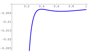
Figure 1: Plots for $P^{\prime}(0)$, Eq. (45), as a function of $r$ are shown for $\delta=0.01$. The red and blue curves correspond to the truncation of the $j$-summation at $j_{\rm max}=10$ and $j_{\rm max}=50$, respectively.

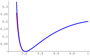
Figure 2: Plots of the derivative $(d/ds)(\sum_{j}G\Delta)(s)|_{s\to 0}$, Eq. (35), as a function of $r$ are shown for $\delta=0.01$. The red and blue curves correspond to the truncation of the $j$-summation at $j_{\rm max}=10$ and $j_{\rm max}=50$, respectively.

The analytic continuation of the counterterms $\sum_{j}G(j,s)\Delta(j,s)$ is discussed in Appendix B, where after considering the $j=0$, $j=1$ and $j\geq 2$ modes separately we find (see App. B)

$$\frac{d}{ds}\sum_{j=0}^{\infty}\Big{(}G(j,s)\Delta(j,s)\Big{)}\Big{|}_{s=0}=\frac{d}{ds}\Big{(}G(0,s)\Delta(0,s)\Big{)}\Big{|}_{s=0}+\frac{d}{ds}\Big{(}G(1,s)\Delta(1,s)\Big{)}\Big{|}_{s=0}+\sum_{j=2}^{\infty}\frac{d}{ds}\Big{(}G(j,s)\Delta(j,s)\Big{)}\Big{|}_{s=0}$$ (35)

In Fig. 2 we plot Eq. (35) as a function of $r$. The $j$-summation truncated at $j_{\rm max}=10$ already exhibits good convergence and coincides well with that for $j_{\rm max}=50$. In the following calculations, we use $j_{\rm max}=50$ as a conservative choice.

We finish this section by noting that the above, quite involved mathematics have yielded in the end very precise numerical results. We will now take advantage of them by considering their implication —e.g., those of the Casimir corrections from bulk fields— for the phenomenological predictions that were mentioned in the first section.

IV Implications for the hierarchy problem

We can now consider the physical implications on the brane in the original 6D theory given by Eq. (2). In Ref mns , several phenomenological applications have been discussed, i.e., to the hierarchy problem and the vacuum (Casimir) energy density (i.e., the effective 4D cosmological constant) on the branes. With our new results at hand, we give a revised version of them, especially focusing on the hierarchy problem. After analysing the hierarchy problem, we briefly discuss the case of the vacuum energy density.

In the original six-dimensional model, the effective four-dimensional Planck scale is

$$M_{\rm pl}^{2}\simeq\frac{\rho_{+}(2\pi-\delta_{+})}{g_{0}^{2}}M_{6}^{4}\,.$$ (36)

If we assume a brane localized field whose bare mass is given by $m^{2}$ on either brane at $\rho_{\pm}$ then the observed mass scales are $m_{+}^{2}=m^{2}$ and $m_{-}^{2}=r^{2}m^{2}\,$. Thus, the mass ratio between the field and the effective Planck mass is given by

$$\frac{m_{\pm}^{2}}{M_{\rm pl}^{2}}\simeq\frac{\mu^{2}m^{2}}{M_{6}^{4}}\ \frac{g_{0}^{2}}{2\pi-\delta_{+}}e^{-(2A_{6}+B_{6})/(2B_{6})}\,,$$ (37)

where $A_{6}$ and $B_{6}$ correspond to $A_{4}$ and $B_{4}$ in the 6D model, respectively. Assuming the factor $(\mu m/M_{6}^{2})^{2}$ takes an optimal value of ${\cal O}(1)$ at the unification of the fundamental scales, then the mass ratio becomes

$$\frac{g_{0}^{2}}{2\pi-\delta_{+}}e^{-(2A_{6}+B_{6})/(2B_{6})}\,,$$ (38)

where we have used the value of $\rho_{+}$, at stabilization. The corresponding quantity in the 4D toy model is given by

$$R(r,\delta_{+})=\frac{g^{2}}{2\pi-\delta_{+}}e^{-(A_{4}+B_{4})/B_{4}}\,.$$ (39)

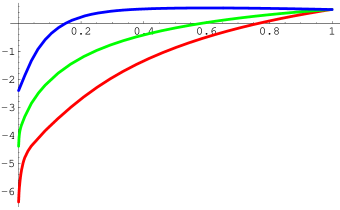
Figure 3: Numerical plots of $\log_{10}R(r,\delta_{+}=0.01)$ as a function of $r$ are shown for $g=0.5,5,50$ (the red, green and blue curves, respectively). We set $j_{\rm max}=n_{\rm max}=50$ as a conservative choice.

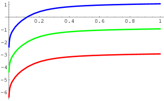
Figure 4: Numerical plots of $\log_{10}R(r,\delta_{+}=0.01)$, via the WKB approximation, as a function of $r$ are shown for $g=0.5,5,50$ (red, green and blue curves, respectively).

In Fig. 3 we have plotted $\log_{10}\big{[}R(r,0,01)\big{]}$ as a function of $r$. The resulting ratios between the scalar and gravitational energies lead to the same conclusions as in the analysis given in Ref. mns , in which the derivative of the zeta function was evaluated by the WKB method (See Fig. 4). Namely, we obtain larger mass hierarchies for smaller $r$ and smaller $g$; in detail, however, the form of $R$ is not the same. The most important difference is the behavior at $r=1$: in the exact spectrum $R$ does not depend on the coupling $g$ (whereas in the WKB approximation it scales as $g^{2}$). Numerical plots also show that this feature is almost independent of the value of the deficit angle $\delta_{+}$. Thus, the expected mass hierarchy in the rugby-ball frame is independent of the value of the dilaton coupling $g$, which is actually the bulk cosmological constant, because the dilaton dynamics are absent in the conformal (rugby-ball) frame.

Finally, we add a few comments on the Casimir energy density realized on the branes, i.e., the effective 4D cosmological constant. As shown in Eq. (56) (also see (57)), the expression for the vacuum energy density has a very similar form to $R$, since $B_{4}(r,\delta_{+})\propto g^{2}$. In fact, after setting $\mu=M_{4}$ as an optimal choice, numerical plots of Eq. (57) in Ref. mns as a function of $r$ for different dilaton coupling $g$ again show convergence to the same point in the $r\to 1$ limit, though here we do not present these results explicitly. For smaller $r$, the same behavior as in Fig. 5 in mns is obtained and implies a tiny amount of effective cosmological constant on the branes, in comparison with the gravitational energy scale $M_{4}^{2}$. The only problem is that the sign of the energy density becomes negative, as is expected from the form of the effective potential Eq. (1). This fact requires an additional uplifting mechanism for the effective potential.

V Conclusion

In this article, we have given a precise analysis of the mode summation in deriving the one-loop effective potential for the volume modulus in a 4D analogue model of a warped flux compactification based on 6D supergravity. In mns the mass spectrum was found using the leading order WKB approximation. Strictly speaking, this is only an approximation and an exact one-loop analysis of the mass spectrum has been performed in the present paper, by employing zeta function regularization techniques. We would also like to stress that the unwarped frame is not the standard Kaluza-Klein spacetime, because of the presence of conical singularities.

In this paper we used our results to look at the hierarchy problem in warped flux compactification models. The qualitative features in Fig. 3 are similar to those of Fig. 4: we expect a larger mass hierarchy for smaller $r$ (where $r$ is the degree of warping) and for larger bulk dilaton coupling $g$. Indeed, for $r\ll 1$, the contribution from the cocycle function becomes important and gives rise to a large mass hierarchy on the brane, though at the same time the effective mass of the modulus may become lighter (and hence more unstable to KK perturbations). However, quantitatively there is a significant difference for $r\lesssim 1$, where quite surprisingly all the curves for different values of $g$ in Fig. 3 converge to the same point at $r=1$. In Fig. 4, which is for the WKB approximation, the behavior of $R$ is proportional to $g^{2}$, even at $r=1$. This may well represent a non-trivial feature of the Casimir effect in the rugby ball limit. Similar results are obtained in the case of the vacuum (Casimir) energy density on the branes, namely convergence to the same value in the $r\to 1$ limit, independently of $g$. For smaller values of $r$, we can expect a tiny amount of the effective cosmological constant on the branes, in comparison with the gravitational energy scale. The negativity of the energy density may require slight modifications of the background model.

As a consistency check of our results, in Figs. 5 and 6 we have plotted the integrands of $\zeta(0)$ and $B_{4}(r,\delta_{+})$, which are related to $a_{4}(f=1)$ given in Eq. (15), as functions of $g$ and $r$, respectively, for a fixed value of the deficit angle, $\delta_{+}$. Note that both quantities are practically insensitive to $\delta_{+}$. In the unwarped frame, due to the properties of the heat kernel coefficients (see e.g., VSV ), the equation $\zeta(0)=a_{4}(f=1)$ should be satisfied. Although they do not agree exactly, they do exhibit a similar behavior, namely increasing for larger $g$ and for smaller $r$. We thus conclude that our results are physically reliable. Nevertheless, there are still slight differences between these values and it is worthwhile to consider the possible origin of this difference.

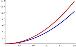
Figure 5: Numerical plot of the integrand of $\zeta(0)$ and $2B_{4}$ as functions of $g$ are shown for $r=1$ and $\delta_{+}=0.01$. The red and blue curves correspond to the cases of $\zeta(0)$ and $2B_{4}$, respectively. We set $j_{\rm max}=n_{\rm max}=50$.

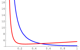
Figure 6: Numerical plot of the integrand of $\zeta(0)$ and $2B_{4}$ as functions of $r$ are shown for $g=10$ and $\delta_{+}=0.01$. The red and blue curves correspond to the cases of $\zeta(0)$ and $2B_{4}$, respectively. We set $j_{\rm max}=n_{\rm max}=50$.

In mns the authors confirmed that $B_{4}$ (and thus $a_{4}(f=1)$) is independent of the value of $\epsilon$ VSV , which characterizes the conformal transformation given in Eq. (7) and therefore, we believe that $B_{4}$ is correct. We have also carefully checked the convergence of the mode summations. Thus, it is the view of the authors that a possible origin for the disagreement could be in our determination of the exact mode spectrum. By imposing vanishing conditions for the mode functions and their derivatives at the poles (branes), we were able to derive the mass spectrum in the rugby-ball frame. Our method to determine the mass spectrum is essentially based on the same arguments given in Parameswaran:2006db , where two conditions, normalizability and regularity at the poles were imposed (more precisely, it was demanded that the wave functions should be Hermitian). However, if only normalizability were imposed, this would allow for logarithmic divergences at the poles and this may well lead to additional modes in the eigenvalue spectrum, which could then reflect in the differences between Figs. 5 and 6. Regardless of this, based on the qualitative behavior of $B_{4}$ and $\zeta(0)$, the existence of such modes does not seem likely to significantly affect the qualitative behavior of our results.

In closing we would also like to stress that although the results presented here are strictly for a toy 4D warped flux compactification model, the methods introduced can be generalized straightforwardly to six dimensions. However, as discussed in mns , to start with the relevant heat kernel coefficient on the cone in six dimensions should be found. In addition, in the current investigation we have focused on the simplest case: a massless, minimally coupled scalar field. It should be also possible to extend our analysis to the case of a bulk scalar field with self interactions and other fields in the multiplets appearing in the supergravity model, which our model is based on. We hope to report on the results of these extended analyses in the near future.

Appendix A Asymptotic expansion of the zeta function

In order to isolate the divergent behavior in the zeta function, due to small $s$, we need to expand Eq. (III.1). Towards this end we shall make use of the asymptotic expansion of the Hurwitz zeta function ElizaldeBook :

$$\zeta_{H}(2s+2j-2,\frac{1}{2}+\frac{1+r}{2\kappa}n) = \frac{1}{2s+2j-3}\Big{(}\frac{1}{2}+\frac{(1+r)n}{2\kappa}\Big{)}^{-(2s+2j-3)}+\frac{1}{2}\Big{(}\frac{1}{2}+\frac{(1+r)n}{2\kappa}\Big{)}^{-(2s+2j-3)-1}$$ (40)

$$+ \frac{1}{2s+2j-3}\sum_{k=2}^{\infty}\frac{B_{k}}{k!}(2s+2j-3)_{k}\left(\frac{1}{2}+\frac{1+r}{2\kappa}n\right)^{-(2s+2j-3)-k}\,,$$

where the $B_{k}$ are Bernoulli numbers. Furthermore, in the limit of large $n$ and fixed $j$, the asymptotic expansion of $\zeta_{H}$ is found to be

$$\zeta_{H}(2s+2j-2,\frac{1}{2}+\frac{1+r}{2\kappa}n)\Big{[}\frac{n^{2}}{\kappa^{2}}(1-r)^{2}+1\Big{]}^{j}\simeq F(n,j;s),$$ (41)

where

$$F(n,j;s):=\frac{n^{-1-2s}}{\kappa^{-1-2s}}{(1-r)^{2j}\over(1+r)^{1+2j+2s}}\frac{2^{-6+2j+2s}}{45(2s+2j-3)}\ \Big{(}w_{0}\frac{n^{4}}{\kappa^{4}}+w_{2}\frac{n^{2}}{\kappa^{2}}+w_{4}\Big{)}\,,$$ (42)

and we have defined

$$w_{0}(j,s) = 360(1+r)^{4}\,,$$

$$w_{2}(j,s) = \frac{360j(1+r)^{4}}{(1-r)^{2}}-60(1+r)^{2}(-3+2s+2j)(-2+2s+2j)\,,$$

$$w_{4}(j,s) = \frac{180(j-1)j(1+r)^{4}}{(1-r)^{4}}-\frac{60j(1+r)^{2}(-3+2j+2s)(-2+2s+2j)}{(1-r)^{2}}$$ (43)

$$+ 7(-3+2s+2j)(-2+2s+2j)(-1+2s+2j)(2s+2j)\,.$$

Note the form of these terms, especially $w_{4}$, will be important for the analytic continuation of the zeta-function.

Appendix B Analytic continuation

In this appendix we discuss the analytic continuation of the various functions discussed in the main text. The expression for the analytic continuation of $\zeta(s)$ to $s\to 0$ is given by

$$\zeta(0) = \frac{g^{2}}{\pi}\int d^{2}x\sum_{n=1}^{\infty}\Big{[}-4\Big{(}\zeta_{H}(-2,\frac{1}{2}+\frac{1+r}{2\kappa}n)-F(n,0,0)\Big{)}+\Big{(}\zeta_{H}(0,\frac{1}{2}+\frac{1+r}{2\kappa}n)\big{(}\frac{n^{2}}{\kappa^{2}}(1-r)^{2}+1\big{)}-F(n,1,0)\Big{)}\Big{]}$$ (44)

$$+ \frac{\kappa g^{2}}{720\pi(1+r)}\int d^{2}x\Big{[}\Big{(}\frac{(1+r)^{4}}{\kappa^{4}}-\frac{(1+r)^{2}}{\kappa^{2}}-14\Big{)}-\frac{(1-r)^{2}}{(1+r)^{2}}\Big{(}\frac{3(1+r)^{4}}{\kappa^{4}}+\frac{3(1+r)^{4}}{(1+r)^{2}}\kappa^{2}-14\Big{)}$$

$$+ \sum_{j=2}^{\infty}\frac{(1-r)^{2j}}{(2j-3)(1+r)^{2j}}\Big{(}90\frac{(1+r)^{4}}{(1-r)^{4}}-60\frac{(1+r)^{2}}{(1-r)^{2}}(2j-3)+14(2j-3)(2j-1)\Big{)}\Big{]}\,.$$

Note that the axisymmetric modes do not contribute to $\zeta(0)$.

We next discuss the analytic continuation that is required to derive the expression for $\zeta^{\prime}(0)$. The analytic continuation of $P^{\prime}(s)$ to $s\to 0$ is given by

$$P^{\prime}(0) = \frac{(2g)^{2}}{\pi}\Big{\{}\Big{(}2\ln(2g)-1\Big{)}\sum_{n=1}^{\infty}\Big{[}\zeta_{H}(-2,\frac{1}{2}+\frac{1+r}{2\kappa}n)-F[n,0;0]\Big{]}$$ (45)

$$- \frac{\ln(2g)}{2}\sum_{n=1}^{\infty}\Big{[}\zeta_{H}(0,\frac{1}{2}+\frac{1+r}{2\kappa}n)\Big{(}\frac{n^{2}}{\kappa^{2}}(1-r)^{2}+1\Big{)}-F[n,1;0]\Big{]}$$

$$- \sum_{n=1}^{\infty}\Big{[}2\zeta_{H}{}^{\prime}(-2,\frac{1}{2}+\frac{1+r}{2\kappa}n)-\partial_{s}F[n,0;s]\Big{|}_{s\to 0}\Big{]}$$

$$+ \frac{1}{4}\sum_{n=1}^{\infty}\Big{[}2\zeta_{H}{}^{\prime}(0,\frac{1}{2}+\frac{1+r}{2\kappa}n)\Big{(}\frac{n^{2}}{\kappa^{2}}(1-r)^{2}+1\Big{)}-\partial_{s}F[n,1;s]\Big{|}_{s\to 0}\Big{]}$$

$$+ \sum_{j=2}^{\infty}\frac{2^{-2j}}{j(j-1)}\sum_{n=1}^{\infty}\Big{(}\zeta_{H}(2j-2,\frac{1}{2}+\frac{1+r}{2\kappa}n)\Big{(}\frac{n^{2}}{\kappa^{2}}(1-r)^{2}+1\Big{)}^{j}-F[n,j;0]\Big{)}\Big{\}}\,.$$

Note, we must also pay attention to the counterterms. The product $G(j,s)\Delta(j,s)$ can be written as

$$G(j,s)\Delta(j,s) = \frac{1}{2^{4}\pi}\frac{\Gamma(s+j-1)}{\Gamma(s)j!}\frac{g^{2(1-s)}\kappa^{1+2s}(1-r)^{2j}}{(1+r)^{1+2s+2j}}\frac{1}{45(2s+2j-3)}\int d^{2}x$$ (46)

$$\times \Big{(}w_{0}(j,s)\frac{\zeta_{R}(2s-3)}{\kappa^{4}}+w_{2}(j,s)\frac{\zeta_{R}(2s-1)}{\kappa^{2}}+w_{4}(j,s)\zeta_{R}(2s+1)\Big{)}\,,$$

where, as before, we must consider the $j=0$, $j=1$ and $j\geq 2$ modes separately. The contribution from the $j=0$ mode is the simplest one, and analytic continuation to $s=0$ results in

$$\frac{d}{ds}\Big{(}G(0,s)\Delta(0,s)\Big{)}\Big{|}_{s\to 0} = \frac{1}{2^{4}\pi}\frac{1}{135}\frac{g^{2}\kappa}{(1+r)}\int d^{2}x\Big{\{}\Big{(}-\frac{1}{s-1}-\frac{2}{2s-3}+2\ln\Big{(}\frac{\kappa}{g(1+r)}\Big{)}\Big{)}$$

$$\times \Big{(}w_{0}(0,0)\frac{\zeta_{R}(-3)}{\kappa^{4}}+w_{2}(0,0)\frac{\zeta_{R}(-1)}{\kappa^{2}}+w_{4}(0,s)\zeta_{R}(2s+1)\Big{|}_{s\to 0}\Big{)}$$

$$+ w_{0}(0,0)\frac{2\zeta_{R}{}^{\prime}(-3)}{\kappa^{4}}+w_{2}{}^{\prime}(0,0)\frac{\zeta_{R}(-1)}{\kappa^{2}}+2w_{2}(0,0)\frac{\zeta_{R}{}^{\prime}(-1)}{\kappa^{2}}$$

$$+ \partial_{s}\Big{(}w_{4}(0,s)\zeta_{R}(2s+1)\Big{)}\Big{|}_{s\to 0}\Big{\}}$$

$$= \frac{1}{2^{4}\pi}\frac{1}{135}\frac{g^{2}\kappa}{(1+r)}\int d^{2}x\Big{\{}\Big{(}\frac{5}{3}+2\ln\Big{(}\frac{\kappa}{g(1+r)}\Big{)}\Big{)}\Big{(}3\frac{(1+r)^{4}}{\kappa^{4}}+30\frac{(1+r)^{2}}{\kappa^{2}}-42\Big{)}$$

$$-50\frac{(1+r)^{2}}{\kappa^{2}}+\frac{720(1+r)^{4}}{\kappa^{4}}\zeta_{R}{}^{\prime}(-3)-\frac{720(1+r)^{2}}{\kappa^{2}}\zeta_{R}{}^{\prime}(-1)+14(11-6\gamma)\Big{\}}\,,$$

where we have used the fact that

$$w_{4}(0,s)\zeta_{R}(2s+1)=-42+14(11-6\gamma)s+O(s^{2})\,.$$ (48)

Similar steps follow for the $j=1$ mode. By setting $j=1$ in $G(j,s)\Delta(j,s)$, differentiating with respect to $s$, and then taking the analytic continuation as $s\to 0$, we obtain

$$\frac{d}{ds}\Big{(}G(1,s)\Delta(1,s)\Big{)}\Big{|}_{s\to 0} = -\frac{1}{2^{4}\pi}\frac{1}{45}\frac{g^{2}\kappa(1-r)^{2}}{(1+r)^{3}}\int d^{2}x\Big{\{}\Big{(}2+2\ln\Big{(}\frac{\kappa}{g(1+r)}\Big{)}\Big{)}$$ (49)

$$\times \Big{(}3\frac{(1+r)^{4}}{\kappa^{4}}-30\frac{(1+r)^{4}}{\kappa^{2}(1-r)^{2}}-14+\frac{60(1+r)^{2}}{(1-r)^{2}}\Big{)}$$

$$-10\frac{(1+r)^{2}}{\kappa^{2}}+\frac{720(1+r)^{4}}{\kappa^{4}}\zeta_{R}{}^{\prime}(-3)+\frac{720(1+r)^{4}}{\kappa^{2}(1-r)^{2}}\zeta_{R}{}^{\prime}(-1)$$

$$-14-\frac{120(1+r)^{2}}{(1-r)^{2}}+\gamma\Big{(}-28+\frac{120(1+r)^{2}}{(1-r)^{2}}\Big{)}\Big{\}}\,,$$

where we have used the expansion around $s=0$:

$$w_{4}(1,s)\zeta_{R}(2s+1)=-14+\frac{60(1+r)^{2}}{(1-r)^{2}}+\Big{[}-14-\frac{120(1+r)^{2}}{(1-r)^{2}}+\gamma\Big{(}-28+\frac{120(1+r)^{2}}{(1-r)^{2}}\Big{)}\Big{]}s+O(s^{2})\,.$$ (50)

For the modes with $j\geq 2$, we obtain

$$\sum_{j=2}^{\infty}\frac{d}{ds}\Big{(}G(j,s)\Delta(j,s)\Big{)}\Big{|}_{s\to 0}$$ (51)

$$= \frac{1}{2^{4}\pi}\sum_{j=2}^{\infty}\frac{1}{45j(j-1)(2j-3)}\frac{g^{2}\kappa(1-r)^{2j}}{(1+r)^{1+2j}}\int d^{2}x$$

$$\times \Big{\{}\Big{[}\psi(j-1)-\frac{2}{2j-3}+2\ln\Big{(}\frac{\kappa}{g(1+r)}\Big{)}\Big{]}\Big{(}{w_{4}(j,s)\zeta_{R}(2s+1)\over\Gamma(s)}\Big{)}\Big{|}_{s\to 0}$$

$$+ w_{0}(j,0)\frac{\zeta_{R}(-3)}{\kappa^{4}}+w_{2}(j,0)\frac{\zeta_{R}(-1)}{\kappa^{2}}+\frac{1}{2}w_{4}(j,0)+\frac{1}{2}\Big{(}3\gamma w_{4}(j,0)+\partial_{s}w_{4}(j,s)\Big{|}_{s\to 0}\Big{)}\Big{\}}$$

$$= \frac{1}{2^{4}\pi}\sum_{j=2}^{\infty}\frac{1}{45j(j-1)(2j-3)}\frac{g^{2}\kappa(1-r)^{2j}}{(1+r)^{1+2j}}\int d^{2}x$$

$$\times \Big{\{}\Big{[}\psi(j-1)-\frac{2}{2j-3}+2\ln\Big{(}\frac{\kappa}{g(1+r)}\Big{)}\Big{]}$$

$$\times 2j(j-1)\Big{(}7(-3+2j)(-1+2j)-\frac{30(-3+2j)(1+r)^{2}}{(1-r)^{2}}+\frac{45(1+r)^{4}}{(1-r)^{4}}\Big{)}$$

$$+ \frac{3(1+r)^{4}}{\kappa^{4}}+\frac{5(1+r)^{2}\big{[}6+4j^{2}-8j\frac{2+r(-1+2r)}{(1-r)^{2}}\big{]}}{\kappa^{2}}$$

$$+ \frac{2}{(1-r)^{4}}\Big{[}-21(1-r)^{4}+84\gamma(1-r)^{4}j^{4}-16j^{3}(1-r)^{2}\Big{(}-7(1-r)^{2}+9\gamma\big{(}3+r(-1+3r)\big{)}\Big{)}$$

$$- 4j\Big{(}-2(1-r)^{2}(38+r(-1+38r))+9\gamma\big{(}13+r(8+r(18+r(8+13r))\big{)}\Big{)}$$

$$+ 12j^{2}\Big{(}-(1-r)^{2}\big{(}31+\gamma(-22+31r)\big{)}+4\gamma\Big{(}17+\gamma(-8+r(27+r(-8+17r)))\Big{)}\Big{)}\Big{]}\Big{\}}\,,$$

where in the first step we used that fact that

$$\left[\frac{w_{4}(j,s)\zeta(2s+1)}{\Gamma(s)}\right]^{\prime}=\frac{1}{2}w_{4}^{\prime}(j,0)+\frac{3}{2}\gamma w_{4}(j,0)\,.$$ (52)

Appendix C Contribution from the axisymmetric modes

The $n=0$ mode, $\lambda_{m0}$, can be treated independently as follows. Using the binomial expansion, we straightforwardly obtain

$$\zeta_{0}(s) = \int d^{2}x\frac{(2g)^{2(1-s)}}{2\pi(s-1)}\sum_{m=1}^{\infty}\Big{[}(m+\frac{1}{2})^{2}-\frac{1}{4}\Big{]}^{1-s}$$ (53)

$$= \int d^{2}x\frac{(2g)^{2(1-s)}}{2\pi}\sum_{j=0}^{\infty}\frac{2^{-2j}\Gamma(j+s-1)}{j!\Gamma(s)}\Big{[}\zeta_{H}(2s+2j-2,\frac{1}{2})-\Big{(}\frac{1}{2}\Big{)}^{2(1-s-j)}\Big{]}\,.$$

This expression requires no further regularization, because the analytic continuation is already built-in to this type of zeta function. The final result is

$$\zeta_{0}{}^{\prime}(0)=\int d^{2}x\,g^{2}\,\frac{\zeta_{R}{}(3)}{\pi^{3}},$$ (54)

where we have used the fact that

$$\sum_{j=2}^{\infty}\frac{2^{-2j}}{j(j-1)}\Big{[}\zeta_{H}(-2+2j,\frac{1}{2})-\big{(}\frac{1}{2}\big{)}^{2(1-j)}\Big{]}=\frac{1}{4}\big{(}-1+\ln 2\big{)}+\frac{7}{8\pi^{2}}\zeta_{R}(3)\,,$$ (55)

and $\zeta_{R}^{\prime}(-2)=-\zeta_{R}(3)/4\pi^{2}$ , which is derived from $\zeta_{R}(z)=\pi^{z-1/2}\zeta_{R}(1-z)[\Gamma((1-z)/2)/\Gamma(z/2)]$. An important observation is that (C2) does not agree with the corresponding expression obtained via the WKB approximation, by a factor of $-3/8$ (see equation (D36) in Ref. mns ).

References

- (1) M. Minamitsuji, W. Naylor and M. Sasaki, JHEP 0612, 079 (2006) [arXiv:hep-th/0606238].
- (2) S. M. Carroll and M. M. Guica, arXiv:hep-th/0302067; I. Navarro, JCAP 0309, 004 (2003) [arXiv:hep-th/0302129]; J. Garriga and M. Porrati, JHEP 0408, 028 (2004) [arXiv:hep-th/0406158]; S. Randjbar-Daemi and V. A. Rubakov, JHEP 0410, 054 (2004) [arXiv:hep-th/0407176]; H. M. Lee and A. Papazoglou, Nucl. Phys. B 705, 152 (2005) [arXiv:hep-th/0407208]; S. Mukohyama, Y. Sendouda, H. Yoshiguchi and S. Kinoshita, JCAP 0507, 013 (2005) [arXiv:hep-th/0506050].
- (3) G. W. Gibbons, R. Guven and C. N. Pope, Phys. Lett. B 595, 498 (2004) [arXiv:hep-th/0307238]; Y. Aghababaie et al., JHEP 0309, 037 (2003) [arXiv:hep-th/0308064]; C. P. Burgess, F. Quevedo, G. Tasinato and I. Zavala, JHEP 0411, 069 (2004) [arXiv:hep-th/0408109].
- (4) C. de Rham and A. J. Tolley, JCAP 0602, 003 (2006) [arXiv:hep-th/0511138].
- (5) M. Peloso, L. Sorbo and G. Tasinato, Phys. Rev. D 73, 104025 (2006) [arXiv:hep-th/0603026]; E. Papantonopoulos, A. Papazoglou and V. Zamarias, arXiv:hep-th/0611311.
- (6) B. M. N. Carter, A. B. Nielsen and D. L. Wiltshire, JHEP 0607, 034 (2006) [arXiv:hep-th/0602086].
- (7) H. M. Lee and A. Papazoglou, Nucl. Phys. B 747, 294 (2006) [arXiv:hep-th/0602208]; C. P. Burgess, C. de Rham, D. Hoover, D. Mason and A. J. Tolley, arXiv:hep-th/0610078.
- (8) H. Yoshiguchi, S. Mukohyama, Y. Sendouda and S. Kinoshita, JCAP 0603, 018 (2006) [arXiv:hep-th/0512212]; Y. Sendouda, S. Kinoshita and S. Mukohyama, Class. Quant. Grav. 23, 7199 (2006) [arXiv:hep-th/0607189]; B. Himmetoglu and M. Peloso, arXiv:hep-th/0612140.
- (9) M. R. Douglas and S. Kachru, arXiv:hep-th/0610102; F. Denef, M. R. Douglas and S. Kachru, arXiv:hep-th/0701050.
- (10) C. P. Burgess, C. Nunez, F. Quevedo, G. Tasinato and I. Zavala, JHEP 0308, 056 (2003) [arXiv:hep-th/0305211].
- (11) K. Milton, S. D. Odintsov and S. Zerbini, Phys. Rev. D65, 065012 (2002).
- (12) S. L. Parameswaran, S. Randjbar-Daemi and A. Salvio, arXiv:hep-th/0608074.
- (13) C. P. Burgess and D. Hoover, arXiv:hep-th/0504004; D. Hoover and C. P. Burgess, JHEP 0601, 058 (2006) [arXiv:hep-th/0507293];
- (14) E. Elizalde, Commun. Math. Phys. 198 (1998) 83 [arXiv:hep-th/9707257]; J. Comput. Appl. Math. 118, 125 (2000); J. Phys. A34, 3025 (2001); E. Elizalde, S. Nojiri, S. D. Odintsov and S. Ogushi, Phys. Rev. D67, 063515 (2003).
- (15) A. Chodos and E. Myers, Phys. Rev. D 31, 3064 (1985); A. Chodos and E. Myers, Can. J. Phys. 64, 633 (1986); Phys. Rev. D31, 3064 (1985).
- (16) D. V. Vassilevich, Phys. Rept. 388, 279 (2003) [arXiv:hep-th/0306138].
- (17) E. Elizalde, Ten physical applications of spectral zeta functions, Lect. Notes Phys. M35 (Springer, Berlin, 1995); E. Elizalde et al., Zeta regularization techniques with applications (World Scientific, Singapore, 1994)