hep-th/0702097 YITP-07-06 OU-HET 574/2007 Supersymmetry breaking in a warped slice with Majorana-type masses

1 Introduction

The five-dimensional (5D) warped spacetime has various aspects for the physics beyond the standard model from the view point of both the phenomenological and the theoretical studies. For example, a hierarchy between the weak and the Planck scale and ones among the observed quark/lepton masses and mixings can be explained by the localization of graviton [1] and matter fields [2] respectively in an orbifold slice of the 5D anti-de Sitter space, AdS₅. In the theoretical side, four-dimensional (4D) strongly coupled gauge theories can be studied within weakly coupled theories in AdS₅ by the use of so-called AdS/CFT correspondence [3]. Moreover, it is known that a low energy effective theory of strongly coupled heterotic string [4] can be described by 5D supergravity (SUGRA) on a curved background [5].

Among these features, the structure of supersymmetry (SUSY) [6, 7, 8] in an orbifold slice of AdS₅, and the mediation patterns of SUSY breaking from the hidden to the visible sector [9] in such background is particularly interesting. Here we focus on some phenomenological models in a slice of AdS₅ with local SUSY. In the SUGRA framework, the $U(1)_{R}$ gauging is necessary to generate a bulk cosmological constant which makes the background warped. Then we have basically two ways for realization of such warped geometry, which are distinguished from each other by the orbifold $Z_{2}$-parity of the gauge coupling constant for the $U(1)_{R}$ symmetry gauged by the $Z_{2}$-odd graviphoton.

In the case of $Z_{2}$-odd $U(1)_{R}$ gauge coupling, an on-shell SUGRA-matter-Yang-Mills system was constructed [7], and a lot of phenomenological studies have been done so far (see, e.g., [10]). However, in order to embed such nontrivial $Z_{2}$-odd coupling constant into SUGRA, which changes the sign across the orbifold boundaries, we need a four-form Lagrange multiplier [11]. On the other hand, in the $Z_{2}$-even coupling case, almost only the on-shell formulation for pure SUGRA case has been studied [6], even though it seems simpler than the $Z_{2}$-odd coupling case in the sense that it does not require any Lagrange multiplier whose origin is unclear within the framework of 5D SUGRA.

In this paper, we study the latter case, i.e., 5D SUGRA compactified on an orbifold $S^{1}/Z_{2}$ where the $U(1)_{R}$ symmetry is gauged by the graviphoton with $Z_{2}$-even coupling, starting from the off-shell formulation [12, 13]. The off-shell formulation allows us to construct such SUGRA model coupled to an arbitrary number of matter and gauge fields even with boundary terms. Interestingly enough, this model allows the Scherk-Schwarz (SS) twist [14] even in the warped geometry [15], in contrast to the case of $Z_{2}$-odd $U(1)_{R}$ coupling where it is prohibited from the consistency of the theory [16]. In the absence of the SS twist, it is briefly shown in Ref. [13] that SUSY is spontaneously broken in a slice of AdS₅ in the case of $Z_{2}$-even coupling. We reexamine this fact in more general setup, i.e., including the SS twist, and obtain a result that SUSY is always broken irrespective of the value of the SS twist parameter.

A scenario of SS SUSY breaking has been extensively studied in a flat space. In such a case, the SS twist can be interpreted as a Wilson line for some auxiliary gauge field in the off-shell formulation [17, 18], and appears as a radion mediated SUSY breaking [19] in the 4D effective theory. Thus it is not an explicit breaking of SUSY and gives a controllable result. Furthermore we have an interesting correlation between the flavor structures of fermion and sfermion when the hierarchies among quark/lepton masses are consequence of the localization of matter fields [20]. However the effect of the SS twist on the soft SUSY breaking parameters in the warped geometry has not been investigated yet. So we study the structure of SUSY breaking in detail.

The sections of this paper are organized as follows. In Section 2, we show the Lagrangian for the 5D gauged SUGRA with $Z_{2}$-even coupling, based on the off-shell formulation. For generality, we also include the SS twist parameter in the action. In Section 3, we analyze the Killing spinor equations and show that SUSY is spontaneously broken in a slice of AdS₅ irrespective of the value of the twist parameter. In Section 4, we study SUSY breaking structure in detail by computing spectra of the gaugino and the gravitino. Section 5 is devoted to summary and discussions. In Appendix A, we briefly review the off-shell formulation of 5D SUGRA on orbifold derived in Refs. [12, 13].

2 5D gauged supergravity with $Z_{2}$-even coupling

In this section, we show the Lagrangian for 5D SUGRA compactified on an orbifold $S^{1}/Z_{2}$ where the $U(1)_{R}$ symmetry is gauged by the graviphoton with a $Z_{2}$-even gauge coupling. We utilize the off-shell formulation given in Refs. [12, 13] and reviewed in Appendix A, in order to include physical $n_{V}$ vector multiplets and $n_{H}$ hypermultiplets with some superpotential terms at the orbifold boundaries.

The ingredients of the off-shell formulation for our setup is the Weyl multiplet, ($e_{\mu}^{\ m}$, $\psi_{\mu}^{i}$, $V_{\mu}^{ij}$, $b_{\mu}$, $v^{mn}$, $\chi^{i}$, $D$), the vector multiplets, ($M$, $W_{\mu}$, $\Omega^{i}$, $Y^{ij}$)^I and the hypermultiplets, (${\cal A}^{\alpha}_{\ i}$, $\zeta^{\alpha}$, ${\cal F}^{\alpha}_{\ i}$). The index $i=1,2$ is the $SU(2)_{\mbox{\scriptsize\boldmath$U$}}$-doublet index. The Greek subscripts $\mu$, $\nu$, $\ldots$ describe the vector indices for 5D curved space, and the corresponding tangent flat space indices are represented by Roman subscripts $m$, $n$, $\ldots$. These subscripts with under-bar will be used for the 4D space other than the compact fifth dimension $\mu=y$ or $m=4$.

The index $I=0,1,2,\ldots,n_{V}$ labels the vector multiplets, and the $I=0$ multiplet is introduced to yield graviphoton degree of freedom which is included in the on-shell SUGRA (Weyl) multiplet. For hyperscalars ${\cal A}^{\alpha}_{\ i}$, the index $\alpha$ runs over $\alpha=1,2,\ldots,2(n_{C}+n_{H})$ where $n_{C}$ and $n_{H}$ are the numbers of the compensator and the physical hypermultiplets, respectively. Each hyperscalar has a quaternionic structure, and is written as

$$\left(\begin{array}[]{cc}{\cal A}^{2\hat{\alpha}-1}_{\ i=1}&{\cal A}^{2\hat{\alpha}-1}_{\ i=2}\\ {\cal A}^{2\hat{\alpha}}_{\ i=1}&{\cal A}^{2\hat{\alpha}}_{\ i=2}\end{array}\right) = \left(\begin{array}[]{cc}({\cal A}^{\hat{\alpha}}_{+})^{\ast}&{\cal A}^{\hat{\alpha}}_{-}\\ ({\cal A}^{\hat{\alpha}}_{-})^{\ast}&{\cal A}^{\hat{\alpha}}_{+}\end{array}\right),$$ (2.5)

where $\hat{\alpha}=1,\ldots,n_{C}+n_{H}$. In this paper we adopt the single compensator case, $n_{C}=1$, and divide the indices into two pieces such as $\alpha=(a,\underline{\alpha})$ where $a=1,2$ and $\underline{\alpha}=1,2,\ldots,2n_{H}$ are indices for the compensator and the physical hypermultiplets, respectively. The $Z_{2}$-parity assignments for the fields in the above multiplets are summarized in Table 1 in Appendix A. Throughout this paper, we work in a unit of the 5D Planck mass, $M_{5}=1$.

The most general off-shell action for 5D SUGRA on $S^{1}/Z_{2}$ orbifold is given by [12]

$$S = \int d^{4}x\int dy\,\bigg{\{}{\cal L}_{b}+{\cal L}_{f}+{\cal L}_{\rm aux}+\sum_{l=0,\pi}{\cal L}^{(l)}\delta(y-lR)\bigg{\}},$$ (2.6)

where ${\cal L}_{b}$, ${\cal L}_{f}$ and ${\cal L}_{\rm aux}$ are the Lagrangians for the bosonic, fermionic and auxiliary fields, respectively. The ${\cal L}^{(l)}$ stands for the boundary Lagrangian. These are explicitly shown in Eqs. (A.7) and (A.8).

2.1 $U(1)_{R}$ gauging and tensions at boundaries

One of important points to realize the warped background geometry is that cosmological constant terms are included in the Lagrangian, otherwise the background becomes flat. In order to obtain an orbifold slice of AdS₅,

$$ds^{2} = e^{-2\sigma(y)}\eta_{\underline{\mu}\underline{\nu}}dx^{\underline{\mu}}dx^{\underline{\nu}}-dy^{2},\quad\sigma(y)\ =\ k|y|,$$ (2.7)

as a solution of the Einstein equation, the bulk cosmological constant $\Lambda$ must be balanced with the tensions $\Lambda^{(0)}$, $\Lambda^{(\pi)}$ at the boundaries [1]. This is the so-called Randall-Sundrum (RS) relation,

$$\sqrt{-6\Lambda} = \Lambda^{(0)}\ =\ -\Lambda^{(\pi)}.$$ (2.8)

The bulk cosmological constant is generated in SUGRA framework by gauging $R$-symmetry with a $Z_{2}$-odd gauge field. The most economical choice for such gauge field is the graviphoton which always exists in 5D SUGRA.

In the off-shell (superconformal) formulation of 5D SUGRA, the $SU(2)_{R}$ symmetry is realized as a diagonal subgroup of $SU(2)_{\mbox{\scriptsize\boldmath$U$}}\times SU(2)_{C}$, where $SU(2)_{\mbox{\scriptsize\boldmath$U$}}$ is a gauge symmetry of superconformal group which rotates the index $i=1,2$, and $SU(2)_{C}$ is an isometry group which rotates only the compensator index $a=1,2$ (see the $U$ gauge-fixing condition in Eq. (A.5)). The simplest version of such $R$-gauging is a gauging of $U(1)$ subgroup of $SU(2)_{R}$. In this case, the covariant derivative of the compensator field is given by

$$\nabla_{\mu}{\cal A}^{a}_{\ i} = \partial_{\mu}{\cal A}^{a}_{\ i}-B_{\mu}g_{R}(t_{R})^{a}_{\ b}{\cal A}^{b}_{\ i}+\cdots,$$ (2.9)

with

$$t_{R} = i\vec{q}\cdot\vec{\sigma},\qquad|\vec{q}|=1,$$ (2.10)

where $B_{\mu}$ is the graviphoton, $\vec{q}$ is a three-dimensional unit vector that indicates the direction of the gauging, and $\vec{\sigma}=(\sigma_{1},\,\sigma_{2},\,\sigma_{3})$ are Pauli matrices. In general, the orbifold projection is expressed as

$$\Phi^{i}(x,-y) = \Pi Z^{i}_{\ j}\Phi^{j}(x,y).$$ (2.11)

where $\Pi=\pm 1$ is the $Z_{2}$-parity eigenvalue of the field $\Phi$. Without loss of generality, we choose $Z=\sigma_{3}$ in the following. The $Z_{2}$-parity of compensator is assigned such that the diagonal components are even while the off-diagonal ones are odd in Eq (2.5). (See Table 1 in Appendix A.)

Since the graviphoton is $Z_{2}$-odd, the gauge coupling $g_{R}$ associated to the gauging (2.10) has to be $Z_{2}$-odd for $\vec{q}=(0,\,0,\,1)$ while $Z_{2}$-even for $\vec{q}=(q_{1},\,q_{2},\,0)$. Most of the phenomenological studies in a slice of AdS₅ have been done in the case of $\vec{q}=(0,\,0,\,1)$ with $Z_{2}$-odd coupling $g_{R}\propto\epsilon(y)$ where $\epsilon(y)$ is the periodic sign function of the compactified extra coordinate $y$. Such $Z_{2}$-odd coupling can be obtained in a sense dynamically by introducing four-form Lagrange multiplier [11] into the off-shell formulation [12]. This multiplier simultaneously generates tensions at the boundaries proportional to $\partial_{y}\epsilon(y)=2(\delta(y)-\delta(y-\pi R))$, which automatically satisfies the RS relation (2.8). Here $R$ is the radius of the orbifold. Thus, this SUGRA model admits an orbifold slice of AdS₅ as a background solution of the Einstein equation [12]. In fact, this background preserves N=1 SUSY, and thus it realizes a SUSY RS model whose on-shell formulation is provided in Ref. [7].

On the other hand, we do not need such Lagrange multiplier in 5D SUGRA framework in the case of $\vec{q}=(q_{1},\,q_{2},\,0)$ with $Z_{2}$-even $g_{R}$. However, in this case, we have to find some mechanism to generate the tensions at the boundaries because the contribution to the tensions from the Lagrange multiplier no longer exists. In the off-shell formulation, constant pieces in the superpotential at the orbifold boundaries generate such tensions because now the $U(1)_{R}$ symmetry is gauged with $Z_{2}$-even coupling $g_{R}$ which does not vanish at the boundaries.

Thus we introduce $N=1$ invariant constant superpotential terms at the orbifold boundaries,

$$\sum_{l=0,\pi}{\cal L}^{(l)}\delta(y-lR) \supset {\cal L}_{W}\ =\ \sum_{l=0,\pi}\delta(y-lR)[\phi^{3}W^{(l)}]_{F},$$ (2.12)

where $\phi$ is a compensator chiral multiplet induced from the bulk compensator hypermultiplet, whose lowest component is ${\cal A}^{a=2}_{\ i=2}$ and $[\ldots]_{F}$ represents the $F$-term invariant formula of $N=1$ superconformal tensor calculus [13, 21]. The complex constant $W^{(l)}$ is parameterized as $W^{(l)}=w^{(l)}_{2}+iw^{(l)}_{1}$ with real constants $w^{(l)}_{1,2}$. Because ${\cal L}_{W}$ contains a tadpole of the auxiliary field ${\cal F}^{a}_{\ i}$ in the compensator hypermultiplet (as well as of $V_{y}^{ij}$), we rearrange the ${\cal F}$-related part of auxiliary Lagrangian ${\cal L}_{\rm aux}$ shown in Eq. (A.7) and find

$${\cal L}_{W}+{\cal L}_{\rm aux}^{{\cal F}} = {\cal L}_{\rm tension}+{\cal L}_{w}+{\cal L}_{\rm aux}^{{\cal F}}\big{|}_{{\cal F}^{a}_{\ i}\to{\cal F}^{a}_{\ i}+C^{a}_{\ i}},$$ (2.13)

where

$${\cal L}_{\rm tension} = -4e_{(4)}g_{R}M^{I=0}\sum_{l=0,\pi}\delta(y-lR)\big{(}q_{1}w^{(l)}_{2}-q_{2}w^{(l)}_{1}\big{)}\big{|}{\cal A}^{a=2}_{\ i=2}\big{|}^{2},$$ (2.14)

$${\cal L}_{w} = e_{(4)}\sum_{l=0,\pi}\delta(y-lR)(w^{(l)}_{2}+iw^{(l)}_{1})\bigg{[}2{\cal A}^{a=2}_{\ i=2}\big{(}\nabla_{4}{\cal A}+{\cal A}V_{4}-2i\bar{\psi}_{4}\zeta\big{)}^{a=2}_{\ i=1}$$ (2.15)

$$-2\bar{\zeta}_{+}^{\hat{\alpha}=1}{\cal P}_{R}\zeta_{+}^{\hat{\alpha}=1}+4i{\cal A}^{a=2}_{\ i=2}\bar{\psi}_{+}\cdot\gamma{\cal P}_{R}\zeta_{+}^{\hat{\alpha}=1}-2({\cal A}^{a=2}_{\ i=2})^{2}\bar{\psi}_{m+}\gamma^{mn}{\cal P}_{L}\psi_{n+}\bigg{]}+{\rm h.c.}$$

$$+2e\bigg{(}e^{-1}e_{(4)}\sum_{l=0,\pi}\delta(y-lR)\big{|}\vec{w}^{(l)}\big{|}\bigg{)}^{2}({\cal A}^{a=2}_{\ i=2})^{2},$$

$$C^{a}_{\ i} = e^{-1}e_{(4)}\sum_{l=0,\pi}\delta(y-lR)\left(\frac{(M^{I=0})^{-1}W_{4}^{I=0}\mathbf{1}_{2}+{\sigma_{3}}}{1+(M^{I=0})^{-2}(W_{4}^{I=0})^{2}}\right)^{a}_{\ b}(i\vec{w}^{(l)}\cdot\vec{\sigma})^{b}_{\ c}{\cal A}^{c}_{\ i}.$$ (2.16)

Here $e_{(4)}$ is a determinant of the induced 4D vielbein and $\vec{w}^{(l)}=(w_{1}^{(l)},w_{2}^{(l)},0)$. Then, the total Lagrangian is obtained as

$${\cal L} = {\cal L}_{b}+{\cal L}_{f}+{\cal L}_{\rm tension}+{\cal L}_{w}+{\cal L}_{\rm aux}\big{|}_{{\cal F}^{a}_{\ i}\to{\cal F}^{a}_{\ i}+C^{a}_{\ i}}.$$ (2.17)

Therefore the boundary tension is proportional to the constant $w_{1,2}^{(l)}$ and also the gauge coupling $g_{R}$. We successfully obtain an orbifold slice of AdS₅ background if we tune the complex constants $W^{(l)}$ to suitable values satisfying the RS relation (2.8).

As pointed out in Ref. [13], any value of $W^{(l)}$ does not allow a Killing spinor in 4D Poincaré invariant vacuum. This means that SUSY is spontaneously broken in the slice of AdS₅, if we choose the off-diagonal $U(1)_{R}$-gauging $\vec{q}=(q_{1},q_{2},0)$ with $Z_{2}$-even $g_{R}$. This fact was originally pointed out in Ref. [22] in a framework of linear multiplet compensator formalism. Here, notice that this class of theory admits the Scherk-Schwarz (SS) twist even in a warped spacetime [15]. Thus, there might be a possibility that the twist recovers SUSY in a slice of AdS₅. We examine this possibility in Section 3, and show that any value of twist parameter cannot recover SUSY.

2.2 Scherk-Schwarz twist

Before analyzing the Killing spinor equations, we show how to include the SS twist into the previous SUGRA model described by the Lagrangian (2.17).

When we consider the torus compactification of fifth dimension, we have a nontrivial physical parameter (even in the pure SUGRA) called the SS twist [14] or the Wilson line associated to the $SU(2)_{\mbox{\scriptsize\boldmath$U$}}$ symmetry [18]. Such a physical parameter can be introduced in the framework of 5D conformal SUGRA in the following way [15].

The normal (untwisted) $SU(2)_{\mbox{\scriptsize\boldmath$U$}}$ gauge fixing for the compensator scalar is given by

$${\cal A}^{a}_{\ i}\equiv\delta^{a}_{\ i}\sqrt{1+{\cal A}^{\underline{\alpha}}_{\ j}{\cal A}_{\underline{\alpha}}^{\ j}}.$$ (2.18)

The SS twist can be incorporated into the theory by modifying this condition as

$${\cal A}^{a}_{\ i}\equiv\left(e^{i\vec{\omega}\cdot\vec{\sigma}\,f(y)}\right)^{a}_{\ i}\sqrt{1+{\cal A}^{\underline{\alpha}}_{\ j}{\cal A}_{\underline{\alpha}}^{\ j}},$$ (2.19)

where $\vec{\omega}=(\omega_{1},\omega_{2},\omega_{3})$ is the twist vector which determines the magnitude and the direction of the twisting, and $f(y)$ is a gauge fixing function satisfying $f(y+\pi R)=f(y)+\pi$. As shown in Ref. [15], the twist is possible only when the twisting direction is the same as the $U(1)_{R}$ gauging direction, $\left[(\vec{q}\cdot i\vec{\sigma}),\,(\vec{\omega}\cdot i\vec{\sigma})\right]=0$, i.e.,

$$\vec{\omega} = \omega\,(q_{1},q_{2},0),$$ (2.20)

otherwise the resulting Poincaré SUGRA has an inconsistency pointed out in Ref. [16]. This fact can be seen as an explicit mass term for the graviphoton in our framework.

We can go back to the ordinary gauge fixing (2.18) by rotating ${\cal A}^{a}_{\ i}$ for the index $a$. Then, the following additional terms [15] come out,

$$e^{-1}{\cal L}_{\omega} = f^{\prime}(y)(i\vec{\omega}\cdot\vec{\sigma})_{ab}\bigg{\{}\epsilon^{ij}({\cal A}^{a}_{\ j}\nabla_{4}{\cal A}^{b}_{\ i}-{\cal A}^{b}_{\ i}\nabla_{4}{\cal A}^{a}_{\ j})+2i\bar{\zeta}^{b}\gamma^{4}\zeta^{a}$$ (2.21)

$$-4i\bar{\psi}_{m}^{i}\gamma^{4}\gamma^{m}\zeta^{a}{\cal A}^{b}_{\ i}+2i\bar{\psi}_{m}^{(i}\gamma^{m4n}\psi_{n}^{j)}{\cal A}^{b}_{\ j}{\cal A}^{a}_{\ i}-\frac{1}{\cal N}\epsilon^{jk}{V_{4}}^{i}_{\ k}({\cal A}^{b}_{\ i}{\cal A}^{a}_{\ j}+{\cal A}^{b}_{\ j}{\cal A}^{a}_{\ i})\bigg{\}}$$

$$-(f^{\prime}(y)|\vec{\omega}|)^{2}\epsilon^{ij}\epsilon_{ab}{\cal A}^{b}_{\ i}{\cal A}^{a}_{\ j},$$

in the bulk Lagrangian, where $f^{\prime}(y)=(d/dy)f(y)$. In this basis, the total Lagrangian is given by

$${\cal L} = {\cal L}_{b}+{\cal L}_{f}+{\cal L}_{\rm tension}+{\cal L}_{w}+{\cal L}_{\omega}+{\cal L}_{\rm aux}\big{|}_{{\cal F}^{a}_{\ i}\to{\cal F}^{a}_{\ i}+C^{a}_{\ i}},$$ (2.22)

where the compensator is now in the periodic basis which follows the normal gauge fixing (A.5).

2.3 On-shell Lagrangian

The terms containing ${V_{4}}^{ij}$ in the Lagrangian are collected as

$$e^{-1}{\cal L}_{{V_{4}}^{ij}} = \epsilon^{jk}\epsilon_{li}(V_{4}-V_{4\,{\rm sol}})^{i}_{\ k}(V_{4}-V_{4\,{\rm sol}})^{l}_{\ j}+2(A+B)^{j}_{\ i}{V_{4}}^{i}_{\ j},$$ (2.23)

where

$$A^{i}_{\ j} = -\frac{1}{{\cal N}}f^{\prime}(y)\epsilon^{ik}\big{\{}(\omega_{2}-i\omega_{1}){\cal A}^{a=1}_{\ k}{\cal A}^{a=1}_{\ j}+(\omega_{2}+i\omega_{1}){\cal A}^{a=2}_{\ k}{\cal A}^{a=2}_{\ j}\big{\}},$$ (2.24)

$$B^{i}_{\ j} = \left(\begin{array}[]{cc}{\cal A}^{a=2}_{\ i=1}B&{\cal A}^{a=2}_{\ i=2}B\\ -({\cal A}^{a=2}_{\ i=2}B)^{\ast}&({\cal A}^{a=2}_{\ i=1}B)^{\ast}\end{array}\right),$$ (2.27)

and

$$B = e^{-1}e_{(4)}\sum_{l=0,\pi}\delta(y-lR)\,(w_{2}^{(l)}+iw_{1}^{(l)}){\cal A}^{a=2}_{\ i=2}.$$ (2.28)

Here we have used the relations $V^{i=1}_{\ j=1}=(V^{i=2}_{\ j=2})^{\ast}$, $V^{i=1}_{\ j=2}=-(V^{i=2}_{\ j=1})^{\ast}$, and ${\cal A}^{a=1}_{\ i=1}=({\cal A}^{a=2}_{\ i=2})^{\ast}$, ${\cal A}^{a=1}_{\ i=2}=-({\cal A}^{a=2}_{\ i=1})^{\ast}$.

Then we easily find

$$e^{-1}{\cal L}_{{V_{4}}^{ij}} = -\epsilon^{jk}\epsilon_{li}\bigg{\{}-\Big{(}V_{4}-(V_{4\,{\rm sol}}+A+B)\Big{)}^{i}_{\ k}\Big{(}V_{4}-(V_{4\,{\rm sol}}+A+B)\Big{)}^{j}_{\ l}$$ (2.29)

$$\qquad\qquad+2(A+B)^{i}_{\ k}{V_{4\,{\rm sol}}}^{l}_{\ j}+(A+B)^{i}_{\ k}(A+B)^{l}_{\ j}\bigg{\}},$$

and the total Lagrangian (2.22) can be rewritten as

$${\cal L} = {\cal L}_{b}+{\cal L}_{f}+{\cal L}^{\prime}_{\rm tension}+{\cal L}^{\prime}_{w+\omega}+{\cal L}_{\rm aux}\Bigg{|}_{\mbox{\scriptsize$\begin{array}[]{l}{\cal F}^{a}_{\ i}\to{\cal F}^{a}_{\ i}+C^{a}_{\ i}\\ {V_{4}}^{i}_{\ j}\to{V_{4}}^{i}_{\ j}-(A+B)^{i}_{\ j}\end{array}$}},$$ (2.32)

where

$$e^{-1}{\cal L}^{\prime}_{\rm tension} = -4g_{R}M^{I=0}\sum_{l=0,\pi}\delta^{l}(y)\big{(}q_{1}w^{(l)}_{2}-q_{2}w^{(l)}_{1}\big{)}\Big{(}1+{\cal A}_{\underline{\alpha}}^{\ i}{\cal A}^{\underline{\alpha}}_{\ i}\Big{)}$$ (2.33)

$$\qquad+2f^{\prime}(y)\sum_{l=0,\pi}\delta^{l}(y)(\omega_{2}w^{(l)}_{2}+\omega_{1}w^{(l)}_{1})\Big{(}1+{\cal A}_{\underline{\alpha}}^{\ i}{\cal A}^{\underline{\alpha}}_{\ i}\Big{)}^{2},$$

$$e^{-1}{\cal L}^{\prime}_{w+\omega} = \bigg{\{}\sum_{l=0,\pi}\delta^{l}(y)(i\vec{w}^{(l)}\cdot\vec{\sigma})_{ij}+f^{\prime}(y)(i\vec{\omega}\cdot\vec{\sigma})_{ij}\bigg{\}}$$ (2.34)

$$\times\bigg{\{}2i\bar{\zeta}^{\underline{\beta}}\gamma^{4}\zeta^{\underline{\alpha}}{\cal A}_{\underline{\beta}}^{\ j}{\cal A}_{\underline{\alpha}}^{\ i}\Big{(}1+{\cal A}_{\underline{\gamma}}^{\ k}{\cal A}^{\underline{\gamma}}_{\ k}\Big{)}^{-1}+4i\bar{\psi}_{m}^{i}\gamma^{4}\gamma^{m}\zeta^{\underline{\alpha}}{\cal A}_{\underline{\alpha}}^{\ j}$$

$$\qquad+\Big{(}2i\bar{\psi}_{m}^{(i}\gamma^{m4n}\psi_{n}^{j)}-2{\cal A}^{\underline{\alpha}(i}\nabla_{4}{\cal A}_{\underline{\alpha}}^{\ j)}+i{\cal N}_{IJ}\bar{\Omega}^{Ii}\gamma_{4}\Omega^{Jj}\Big{)}\Big{(}1+{\cal A}_{\underline{\beta}}^{\ k}{\cal A}^{\underline{\beta}}_{\ k}\Big{)}\bigg{\}}$$

$$-2\bigg{\{}\sum_{l=0,\pi}\Big{(}\delta^{l}(y)|\vec{w}^{(l)}|\Big{)}^{2}+\Big{(}f^{\prime}(y)|\vec{\omega}|\Big{)}^{2}\bigg{\}}\Big{(}1+{\cal A}_{\underline{\alpha}}^{\ i}{\cal A}^{\underline{\alpha}}_{\ i}\Big{)}{\cal A}_{\underline{\beta}}^{\ j}{\cal A}^{\underline{\beta}}_{\ j},$$

and

$$\delta^{l}(y) = e^{-1}e_{(4)}\delta(y-lR).$$ (2.35)

Note that the above expression is valid under the regularization satisfying $\delta^{l}(y)F(\Phi_{+},\Phi_{-})=\delta^{l}(y)F(\Phi_{+},0)$ for any regular function $F$ of any $Z_{2}$-even and $Z_{2}$-odd fields $\Phi_{+}$ and $\Phi_{-}$.

Taking into account the superconformal gauge fixing conditions (A.5) which result in $M^{I=0}=1+\cdots$ and ${\cal A}^{a}_{\ i}=\delta^{a}_{\ i}+\cdots$, the tensions at the boundaries are written as

$${\cal L}^{\prime}_{\rm tension} = -e_{(4)}\sum_{l=0,\pi}\delta(y-lR)\Lambda^{(l)}+\cdots,$$ (2.36)

$$\Lambda^{(l)} = 2\Big{(}2g_{R}q_{1}-f^{\prime}(lR)\omega_{2}\Big{)}w^{(l)}_{2}-2\Big{(}2g_{R}q_{2}+f^{\prime}(lR)\omega_{1}\Big{)}w^{(l)}_{1},$$ (2.37)

where ellipses stand for field-dependent terms. The bulk cosmological constant $\Lambda$ induced by the $U(1)_{R}$ gauging is found in ${\cal L}_{b}$ as

$${\cal L}_{b} \supset {\cal L}_{\rm c.c.}\ =\ \frac{8}{3}g_{R}^{2}(M^{I=0})^{2}|{\cal A}^{a=2}_{\ i=2}|^{2}\ =\ -\Lambda+\cdots,$$ (2.38)

where $\Lambda=-6k^{2}$ and $k=2g_{R}/3$ is the AdS₅ curvature scale in Eq. (2.7). The ellipsis again stands for field dependent terms. By comparing (2.36) and (2.38), we find that the RS relation (2.8) is satisfied if

$$6k = -\Big{(}-6kq_{1}+2f^{\prime}(0)\omega_{2}\Big{)}w^{(0)}_{2}-\Big{(}6kq_{2}+2f^{\prime}(0)\omega_{1}\Big{)}w^{(0)}_{1}$$ (2.39)

$$= \Big{(}-6kq_{1}+2f^{\prime}(\pi R)\omega_{2}\Big{)}w^{(\pi)}_{2}+\Big{(}6kq_{2}+2f^{\prime}(\pi R)\omega_{1}\Big{)}w^{(\pi)}_{1}.$$

Together with the consistency condition (2.20) for the twist vector $\vec{\omega}$, the relation (2.39) results in

$$1 = (w^{(0)}_{2}q_{1}-w^{(0)}_{1}q_{2})-\frac{\omega}{3k}f^{\prime}(0)(w^{(0)}_{1}q_{1}+w^{(0)}_{2}q_{2})$$ (2.40)

$$= -(w^{(\pi)}_{2}q_{1}-w^{(\pi)}_{1}q_{2})+\frac{\omega}{3k}f^{\prime}(\pi R)(w^{(\pi)}_{1}q_{1}+w^{(\pi)}_{2}q_{2}).$$

For instance, if the $U(1)_{R}$ gauging direction is $\vec{q}=(1,\,0,\,0)$ and the boundary constant superpotentials $W^{(0,\pi)}$ are real, the RS condition (2.40) uniquely determines $W^{(0,\pi)}=w_{2}^{(0,\pi)}$ as

$$w_{2}^{(0)} = -w_{2}^{(\pi)}\ =\ 1.\qquad(q_{2}=0,\,w_{1}^{(0,\pi)}=0)$$ (2.41)

3 Killing spinor equations and SUSY breaking

Now we study the Killing conditions. The gravitino SUSY transformation is given by

$$\delta\psi_{\mu}^{i} = \bigg{(}\partial_{\mu}-\frac{1}{4}\omega_{\mu}^{\ mn}\gamma_{mn}+\frac{1}{2}b_{\mu}\bigg{)}\varepsilon^{i}-{V_{\mu}}^{i}_{\ j}\varepsilon^{j}+\frac{1}{2}v^{mn}\gamma_{\mu mn}\varepsilon^{i}-\gamma_{\mu}\eta^{i},$$ (3.1)

$$\eta^{i} = -\frac{{\cal N}_{I}}{12{\cal N}}\gamma\cdot\hat{F}^{I}(W)\varepsilon+\frac{{\cal N}_{I}}{3{\cal N}}{Y^{I}}^{i}_{\ j}\varepsilon^{j}+\frac{{\cal N}_{IJ}}{3{\cal N}}{\Omega^{I}}^{i}2i\bar{\varepsilon}\Omega^{J},$$ (3.2)

where $\varepsilon^{i}$ is SUSY transformation parameter. To find a Killing spinor in the AdS₅ background (2.7), we substitute the on-shell values of the auxiliary fields into Eq. (3.1), and apply the superconformal gauge fixing conditions (A.5).

From $\delta\psi_{\underline{\mu}}^{i}=0$, we find

$$\frac{1}{3}{\cal N}_{I}{Y^{I}}^{i}_{\ j}\varepsilon^{j} = -\frac{1}{2}\sigma^{\prime}(y)\gamma_{4}\varepsilon^{i},$$ (3.3)

where $\sigma^{\prime}(y)=(d/dy)\sigma(y)=k\epsilon(y)$. This results in

$$\sigma^{\prime}(y)\varepsilon^{i=1}-\frac{2}{3}g_{R}|{\cal A}^{a=2}_{\ i=2}|^{2}M^{I=0}(q_{1}-iq_{2})\gamma_{5}\varepsilon^{i=2} = 0,$$

$$\sigma^{\prime}(y)\varepsilon^{i=2}-\frac{2}{3}g_{R}|{\cal A}^{a=2}_{\ i=2}|^{2}M^{I=0}(q_{1}+iq_{2})\gamma_{5}\varepsilon^{i=1} = 0.$$ (3.4)

Substituting these equations into another condition $\delta\psi_{y}=0$ yields

$$\partial_{y}\varepsilon^{i}-{V_{y}}^{i}_{\ j}\varepsilon^{j}-\frac{1}{2}\sigma^{\prime}(y)\varepsilon^{i} = 0.$$ (3.5)

The transformation parameter $\varepsilon^{i}$ is an $SU(2)$-Majorana spinor, and is recasted as two Majorana spinors $\varepsilon_{+}=\varepsilon^{i=1}_{R}+\varepsilon^{i=2}_{L}$ and $\varepsilon_{-}=i(\varepsilon^{i=1}_{L}+\varepsilon^{i=2}_{R})$, which are $Z_{2}$-even and $Z_{2}$-odd, respectively. Then we obtain a relation between $\varepsilon_{+}$ and $\varepsilon_{-}$ from Eq. (3.4) as

$$\varepsilon_{-} = -(q_{2}-iq_{1}\gamma_{5})\epsilon(y)\varepsilon_{+}.$$ (3.6)

From (3.5) and (3.6), we obtain

$$\left\{\begin{array}[]{lcl}\partial_{y}\tilde{\varepsilon}_{+R}&=&-i(q_{2}-q_{1})({V_{y}}^{i=2}_{\ j=1})^{\ast}\epsilon(y)\tilde{\varepsilon}_{+R},\\[5.0pt] \partial_{y}\tilde{\varepsilon}_{+L}&=&i(q_{2}+iq_{1}){V_{y}}^{i=2}_{\ j=1}\epsilon(y)\tilde{\varepsilon}_{+L},\\[5.0pt] \partial_{y}\big{(}\epsilon(y)\tilde{\varepsilon}_{+R}\big{)}&=&-i(q_{2}+iq_{1}){V_{y}}^{i=2}_{\ j=1}\tilde{\varepsilon}_{+R},\\[5.0pt] \partial_{y}\big{(}\epsilon(y)\tilde{\varepsilon}_{+L}\big{)}&=&i(q_{2}-iq_{1})({V_{y}}^{i=2}_{\ j=1})^{\ast}\tilde{\varepsilon}_{+L},\end{array}\right.$$ (3.11)

where $\tilde{\varepsilon}_{\pm}\equiv e^{-\sigma(y)/2}\varepsilon_{\pm}$.

To have a Killing spinor, ${V_{y}}^{i=2}_{\ j=1}$ must be in the form of

$${V_{y}}^{i=2}_{\ j=1} = (q_{1}+iq_{2})\big{(}-iv+\partial_{y}\epsilon(y)\big{)},$$ (3.12)

where $v$ is a real constant. The on-shell form of $V_{y}=e_{y}^{\ 4}V_{4}$ is determined by Eq. (2.29) and we find

$${V_{y}}^{i=2}_{\ j=1} = (A+B)^{i=2}_{\ j=1},$$ (3.13)

where $A^{i}_{\ j}$ and $B^{i}_{\ j}$ are given in Eq. (2.27). Comparing Eq. (3.13) with Eq. (3.12), we find that, if $f(y)$ is not a singular function,

$$w^{(0)}_{1}=2q_{2},\quad w^{(0)}_{2}=-2q_{1},\quad w^{(\pi)}_{1}=-2q_{2},\quad w^{(\pi)}_{2}=2q_{1},$$ (3.14)

is the condition for preserved SUSY in a slice of AdS₅, which leads to relations,

$$q_{2}w^{(0)}_{1}-q_{1}w^{(0)}_{2} = -(q_{2}w^{(\pi)}_{1}-q_{1}w^{(\pi)}_{2})\ =\ 2(q_{1}^{2}+q_{2}^{2})\ =\ 2,$$ (3.15)

and

$$w^{(0)}_{1}q_{1}+w^{(0)}_{2}q_{2}\ =\ w^{(\pi)}_{1}q_{1}+w^{(\pi)}_{2}q_{2} = 0.$$ (3.16)

From these relations, we find that the RS relation (2.40) is never satisfied for SUSY-preserving parameter choice (3.14), irrespective of the values of twist parameter $\omega$. Note that SUSY might be restored in a detuned case with an AdS₄ background geometry.

4 4D gaugino and gravitino masses

From the analysis of Killing spinor, we have found that SUSY is spontaneously broken in the orbifold slice of AdS₅. The result also shows that the SS twist cannot restore SUSY with vanishing 4D cosmological constant. This is contrast to the situation in the case of $Z_{2}$-odd coupling, where the tensions at the boundaries are automatically supplied by the four-form mechanism generating such an odd coupling constant, and SUSY can be preserved in an orbifold slice of AdS₅.

Because SUSY must be broken with almost vanishing vacuum energy in our real world, the model studied above can be one of interesting mechanisms for such realization. Then, next, we study SUSY breaking structure more precisely by analyzing the 4D superparticle spectrum. For simplicity, we consider the case with a physical Abelian vector multiplet ($n_{V}=1$) with $Z_{2}$-even parity and no physical hypermultiplet ($n_{H}=0$) coupled to SUGRA, and show the lightest masses in the gaugino and gravitino spectra.

The gaugino and gravitino bilinear terms in our model are collected as

$$e^{-1}{\cal L}^{(2)}_{1/2} = 2ia_{IJ}\bar{\Omega}^{Ii}\nabla\!\!\!\!/\,\,\Omega^{J}_{\ i}+2i{\cal N}^{IJ}{\cal N}_{JKL}{\cal A}_{ai}(gt_{I})^{ab}{\cal A}_{bj}\bar{\Omega}^{Ki}\Omega^{Lj}+2ia_{IJ}({\cal A}^{a}_{\ i}\partial_{y}{\cal A}_{aj})\bar{\Omega}^{Ii}\gamma^{y}\Omega^{Jj}$$ (4.1)

$$= i\bar{\Omega}^{i}\nabla\!\!\!\!/\,\,\Omega_{\ i}-i\bar{\Omega}^{i}\bigg{(}\frac{1}{2}m^{(q)}_{ij}-i\gamma_{5}m^{(\omega)}_{ij}\bigg{)}\Omega^{j}+\cdots,$$

$$e^{-1}{\cal L}^{(2)}_{3/2} = -2i\bar{\psi}^{i}_{\mu}\gamma^{\mu\nu\rho}\nabla_{\nu}\psi_{\rho i}-2iM^{I}{\cal A}^{a}_{\ i}(gt_{I})_{ab}{\cal A}^{b}_{\ j}\bar{\psi}^{(i}_{m}\gamma^{mn}\psi^{j)}_{n}-2i{\cal A}^{a}_{\ i}\nabla_{n}{\cal A}_{aj}\bar{\psi}^{(i}_{m}\gamma^{mnk}\psi^{j)}_{k}$$ (4.2)

$$= 2i\bar{\psi}^{i}_{\mu}\gamma^{\mu\nu\rho}\nabla_{\rho}\psi_{\nu i}+2i\bar{\psi}^{(i}_{m}\gamma^{mn}\bigg{(}\frac{3}{2}m^{(q)}_{ij}-i\gamma_{5}m^{(\omega)}_{ij}\bigg{)}\psi^{j)}_{n}+\cdots,$$

where the compensator scalar ${\cal A}^{a}_{\ i}$ is in the twisted basis (2.19). The ellipses denote cubic or higher-order terms, and the mass parameters are given by

$$m^{(q)}_{ij} = k\left(\begin{array}[]{cc}q_{2}-iq_{1}&0\\ 0&q_{2}+iq_{1}\end{array}\right),$$ (4.5)

$$m^{(\omega)}_{ij} = f^{\prime}(y)\left(\begin{array}[]{cc}\omega_{2}-i\omega_{1}&0\\ 0&\omega_{2}+i\omega_{1}\end{array}\right)$$ (4.11)

$$\qquad-\sum_{l=0,\pi}e^{-1}e_{(4)}\delta(y-lR)\left(\begin{array}[]{cc}w^{(l)}_{2}-iw^{(l)}_{1}&0\\ 0&w^{(l)}_{2}+iw^{(l)}_{1}\end{array}\right).$$

Both $\Omega^{i}$ and $\psi^{i}_{\mu}$ are $SU(2)$-Majorana spinors satisfying $\bar{\Omega}^{i}\equiv(\Omega_{i})^{\dagger}\gamma^{0}=(\Omega^{i})^{T}C_{5}$ where $C_{5}$ is a 5D charge conjugation matrix. We can decompose them into two Weyl spinors as, e.g.,

$$\Omega^{i=1} = \left(\begin{array}[]{c}\lambda_{\alpha}\\ -i\bar{\xi}^{\dot{\alpha}}\end{array}\right),\qquad\Omega^{i=2}\ =\ \left(\begin{array}[]{c}-i\xi_{\alpha}\\ \bar{\lambda}^{\dot{\alpha}}\end{array}\right).$$ (4.16)

We rearrange them into usual Majorana spinors $\Omega_{\pm}$ in the $Z_{2}$-eigenstates satisfying $(\Omega_{\pm})^{\dagger}\gamma^{0}=(\Omega_{\pm})^{T}C_{4}$, where $C_{4}$ is a 4D charge conjugation matrix, as

$$\Omega_{+} = \left(\begin{array}[]{c}\lambda_{\alpha}\\ \bar{\lambda}^{\dot{\alpha}}\end{array}\right),\qquad\Omega_{-}\ =\ \left(\begin{array}[]{c}\xi_{\alpha}\\ \bar{\xi}^{\dot{\alpha}}\end{array}\right).$$ (4.21)

These spinors are expanded into Kaluza-Klein (KK) modes as

$$\lambda_{\alpha} = e^{2\sigma(y)}\sum_{n}f^{(+)}_{n}(y)\lambda^{(n)}_{\alpha}(x),$$

$$\xi_{\alpha} = e^{2\sigma(y)}\sum_{n}f^{(-)}_{n}(y)\xi^{(n)}_{\alpha}(x),$$ (4.22)

where complex wavefunctions $f^{(\pm)}_{n}(y)$ are solutions to the following equations,

$$i\partial_{y}f^{(-)}_{n}(y)+e^{\sigma(y)}M_{n}(f^{(+)}_{n}(y))^{\ast}+(\mu^{(1)}_{+}+i\mu^{(2)}_{+})f^{(+)}_{n}(y) = 0,$$

$$i\partial_{y}f^{(+)}_{n}(y)-e^{\sigma(y)}M_{n}(f^{(-)}_{n}(y))^{\ast}-(\mu^{(1)}_{-}+i\mu^{(2)}_{-})f^{(-)}_{n}(y) = 0.$$ (4.23)

Here, $M_{n}$ is the KK mass eigenvalues, and

$$\mu^{(1)}_{\pm} = skq_{1}\pm{\rm Re}\,m^{(\omega)}_{22},$$

$$\mu^{(2)}_{\pm} = \pm skq_{2}-{\rm Im}\,m^{(\omega)}_{22},$$ (4.24)

where $s=1/2,\,3/2$ for gaugino and gravitino, respectively.

For a simple parameter choice (2.41) and a gauge fixing function $f(y)=y/R$, the KK equations (4.23) are written as

$$\partial_{y}a^{(+)}_{n}(y)+(e^{\sigma(y)}M_{n}-sk)a^{(-)}_{n}(y)-(\omega/R)\,b^{(-)}_{n}(y) = 0,$$

$$\partial_{y}a^{(-)}_{n}(y)-(e^{\sigma(y)}M_{n}+sk)a^{(+)}_{n}(y)-(\omega/R)\,b^{(+)}_{n}(y) = 0,$$

$$\partial_{y}b^{(+)}_{n}(y)-(e^{\sigma(y)}M_{n}+sk)b^{(-)}_{n}(y)+(\omega/R)\,a^{(-)}_{n}(y) = 0,$$

$$\partial_{y}b^{(-)}_{n}(y)+(e^{\sigma(y)}M_{n}-sk)b^{(+)}_{n}(y)+(\omega/R)\,a^{(+)}_{n}(y) = 0,$$ (4.25)

where real wavefunctions $a^{(\pm)}_{n}(y)$ and $b^{(\pm)}_{n}(y)$ are defined by

$$f^{(+)}_{n}(y) = a^{(+)}_{n}(y)+ib^{(+)}_{n}(y),$$

$$f^{(-)}_{n}(y) = i(a^{(-)}_{n}(y)+ib^{(-)}_{n}(y)).$$ (4.26)

The boundary conditions can be extracted from the delta-functions in $m^{(\omega)}_{22}$ of Eq. (4.24), and are found in this case as

$$2a^{(-)}_{n}(0+\varepsilon)+a^{(+)}_{n}(0) = 0,$$

$$2a^{(-)}_{n}(\pi R-\varepsilon)+a^{(+)}_{n}(\pi R) = 0,$$

$$2b^{(-)}_{n}(0+\varepsilon)+b^{(+)}_{n}(0) = 0,$$

$$2b^{(-)}_{n}(\pi R-\varepsilon)+b^{(+)}_{n}(\pi R) = 0,$$ (4.27)

where $\varepsilon$ is a positive infinitesimal. Note that $a^{(-)}(y)$ and $b^{(-)}(y)$ are discontinuous at the boundaries.

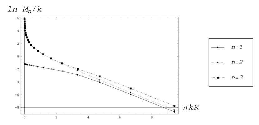
(a) Gaugino: $s=1/2$,  $\omega=0$

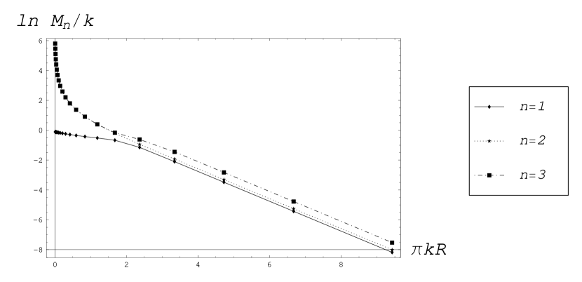
(b) Gravitino: $s=3/2$,  $\omega=0$

Figure 1: Numerical results for (a) the gaugino and (b) the gravitino mass spectra up to the third KK excited modes in terms of a dimensionless quantity $\pi kR$. The parameters in the model are chosen as in Eq. (2.41).

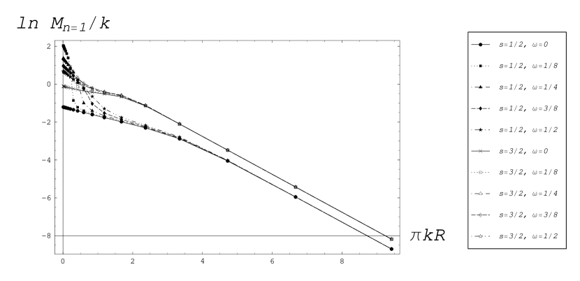
(a) The lightest gaugino ($s=1/2$) and gravitino ($s=3/2$) masses.

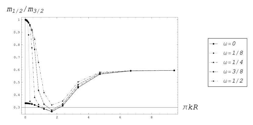
(b) The lightest gaugino/gravitino mass ratio.

Figure 2: Numerical estimation for the effect of the SS twist $\omega$ on the masses of the lightest modes in the gaugino and the gravitino KK spectra. (a) The lightest gaugino and gravitino masses are shown together, and (b) the lightest gaugino/gravitino mass ratio is shown for various values of the SS twist, $\omega$. The parameters in the model are chosen as in Eq. (2.41).

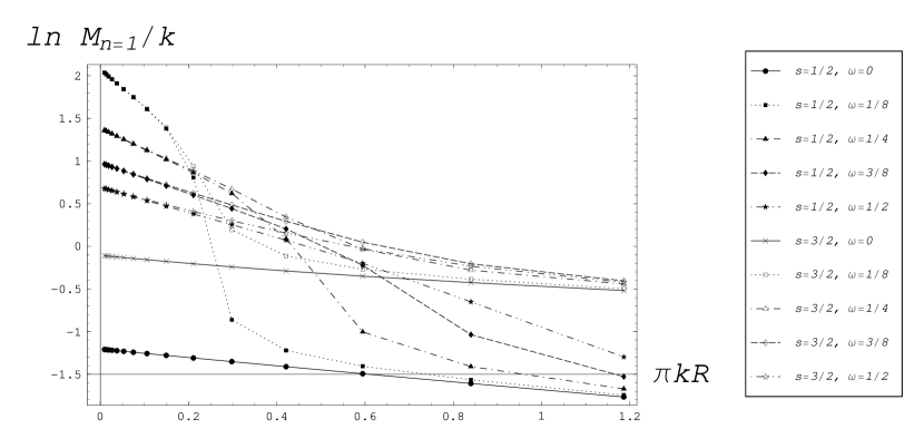
(a) The lightest gaugino ($s=1/2$) and gravitino ($s=3/2$) masses.

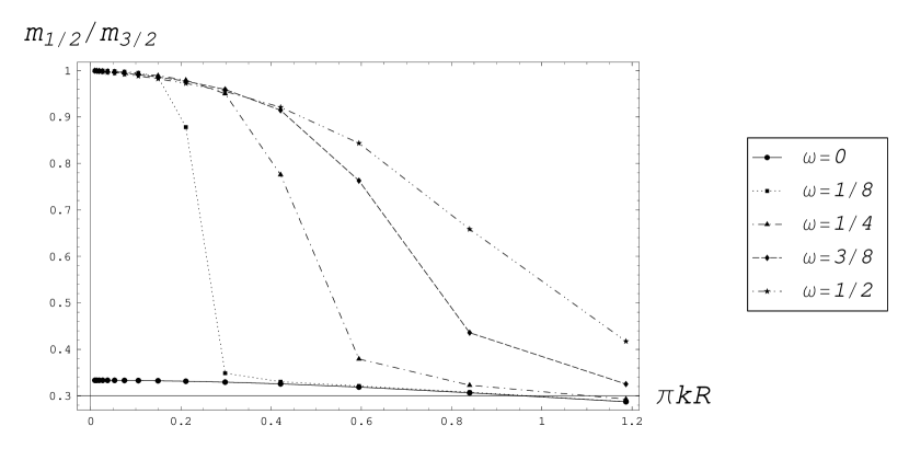
(b) The lightest gaugino/gravitino mass ratio.

Figure 3: The small $\pi kR$ region of Fig. 2 is magnified.

In the case of SUGRA with $Z_{2}$-odd coupling, Dirac-type bulk mass terms such as $\bar{\Omega}_{+}\Omega_{-}$ are generated, which results in the Bessel-type wavefunctions. On the other hand, in the case of $Z_{2}$-even coupling, we have Majorana-type mass terms such as $\bar{\Omega}_{+}\Omega_{+}$, $\bar{\Omega}_{-}\Omega_{-}$. In the latter case, we cannot solve analytically the first-order coupled differential equations (4.25). Therefore, we show some numerical results for the mass eigenvalues in the case of simple parameter choice shown in Eq. (2.41).

In Fig. 1, the $\pi kR$ dependences of the gaugino and gravitino mass spectra are given for $\omega=0$ up to the third KK excited modes. In Fig. 2 (a), the masses of the lightest modes are shown together for $\omega=0,\,1/8,\,1/4,\,3/8,\,1/2$. The small $\pi kR$ region of Fig. 2 (a) is magnified in Fig. 3 (a). From these figures, we find that, for $\pi kR\gg 1$, the lightest gaugino and gravitino masses behave like $m_{1/2},\,m_{3/2}\approx e^{-\pi kR}k$ which is exponentially suppressed as is expected from the highly warped geometry. The effect of the SS twist is negligible in this region. On the other and, it becomes more important in the region $\pi kR<2$.

The overall SUSY breaking scale can be read off from the lightest gravitino mass $m_{3/2}$. The next important quantity is the gaugino/gravitino mass ratio $m_{1/2}/m_{3/2}$, which is shown in Fig. 2 (b). The small $\pi kR$ region of Fig. 2 (b) is magnified in Fig. 3 (b). The ratio takes minimum value at $\pi kR\sim 2$ which is about $0.2$. In the flat limit $k\to 0$, the ratio $m_{1/2}/m_{3/2}$ converges on unity when $\omega\neq 0$. This is the same ratio as in the case of the radion mediation in flat space which is equivalent to the SS SUSY breaking in flat space [18]. When $\omega=0$, SUSY is restored in the flat limit, and both $m_{1/2}$ and $m_{3/2}$ approach to zero.

5 Summary and discussions

We have studied the five-dimensional SUGRA compactified on an orbifold $S^{1}/Z_{2}$ where the $U(1)_{R}$ symmetry is gauged by the graviphoton with $Z_{2}$-even coupling. In order to include superpotential terms at the orbifold boundaries as well as matter fields, we worked in the off-shell formulation of 5D SUGRA. For generality, we have introduced the SS twist parameter in the Lagrangian. After integrating out the auxiliary fields, the on-shell action is obtained including tensions induced by the constant superpotentials at the boundaries, and the Killing spinor equations are derived in an orbifold slice of AdS₅. It has been shown that the equations do not allow a Killing spinor on such background irrespective of the value of twist parameter $\omega$, that means SUSY is spontaneously broken on this background and the SS twist cannot restore it.

We have also shown the details of SUSY breaking when the constant superpotential terms at the boundaries are tuned such that the 4D cosmological constant vanishes. The KK equations for the bulk gaugino and gravitino wavefunctions are derived, which do not have an analytic expressions for the solutions in contrast to the case of SUGRA with $Z_{2}$-odd coupling. This is due to the existence of the Majorana-type bulk mass instead of the Dirac-type. A numerical computation for the KK mass eigenvalues has been performed. The result shows that the 4D (lightest) gaugino and gravitino masses behave as $m_{1/2}$, $m_{3/2}\approx e^{-\pi kR}k$ in the large warping region $\pi kR\gg 1$ that possesses a large exponential suppression, but a negligible effect of the SS twist. On the other hand, the twist provides a sizable effect in the small warping region $\pi kR<2$.

The ratio between the gaugino and the gravitino masses $m_{1/2}/m_{3/2}$ is suppressed at most by a factor of ${\cal O}(1/10)$ within the whole range of warping parameter, $\pi kR$ (at least for the simple parameter choice (2.41)). Then the mediation of SUSY breaking to the gaugino mass will be interpreted as a modulus-dominated one (radion mediation), and the contribution from 4D chiral compensator at the loop level [23] is negligible. However, in the region $\pi kR\gg 1$, the messenger scale can be naturally very low compared to the modulus (radion) mediation in a flat space without fine-tuning. Then, we may realize a low scale modulus mediation without fine-tuning within our framework. For more detailed study about the low energy phenomenology, the 4D effective theory in $N=1$ superspace would be useful. A direct and systematic derivation for such 4D effective action starting from the off-shell SUGRA is given in Ref. [24] based on the $N=1$ superfield description of 5D SUGRA proposed in Ref. [25] and developed in Ref. [26]. An application of these effective action method to the present model will be interesting and instructive.

The orbifold radius remains as a modulus in our simple setup. If we introduce, e.g., some boundary induced potential terms to stabilize the radion, they can generate constant terms in the boundary actions after the radion has a vacuum expectation value. The constant superpotentials on the boundaries in our model may originate from such constant terms. In such sense, the radion stabilization mechanism would have some connection to the SUSY breaking structure studied in this paper.

Acknowledgements

H. A. and Y. S. are supported by the Japan Society for the Promotion of Science for Young Scientists (No.182496 and No.179241, respectively). The numerical calculations were carried out on Sushiki at YITP in Kyoto University.

Appendix A Off-shell formulation of 5D orbifold supergravity

In this appendix we review the hypermultiplet compensator formulation of 5D conformal (off-shell) SUGRA derived in Refs. [12, 13].

The 5D superconformal algebra consists of the Poincaré symmetry $P$, $M$, the dilatation symmetry $D$, the $SU(2)$ symmetry $U$, the special conformal boosts $K$, $N=2$ supersymmetry $Q$, and the conformal supersymmetry $S$. We use $\mu,\nu,\ldots$ as five-dimensional curved indices and $m,n,\ldots$ as the tangent flat indices. The gauge fields corresponding to these generators $\mbox{\boldmath$X$}_{\!\!A}=\mbox{\boldmath$P$}_{m},\,\mbox{\boldmath$M$}_{mn},\,\mbox{\boldmath$D$},\,\mbox{\boldmath$U$}_{ij},\,\mbox{\boldmath$K$}_{m},\,\mbox{\boldmath$Q$}_{i},\,\mbox{\boldmath$S$}_{i}$, are respectively $h_{\mu}^{\ A}=e_{\mu}^{\ m},\,\omega_{\mu}^{mn},\,b_{\mu},\,V_{\mu}^{ij},\,f_{\mu}^{\ m},\,\psi_{\mu}^{i},\,\phi_{\mu}^{i}$, in the notation of Refs. [12, 13]. The index $i=1,2$ is the $SU(2)_{\mbox{\scriptsize\boldmath$U$}}$-doublet index which is raised and lowered by antisymmetric tensors $\epsilon^{ij}=\epsilon_{ij}$.

In this paper we are interested in the following superconformal multiplets:

• 5D Weyl multiplet: ($e_{\mu}^{\ m}$, $\psi_{\mu}^{i}$, $V_{\mu}^{ij}$, $b_{\mu}$, $v^{mn}$, $\chi^{i}$, $D$),

• 5D vector multiplet: ($M$, $W_{\mu}$, $\Omega^{i}$, $Y^{ij}$)^I,

• 5D hypermultiplet: (${\cal A}^{\alpha}_{\ i}$, $\zeta^{\alpha}$, ${\cal F}^{\alpha}_{\ i}$).

Here the index $I=0,1,2,\ldots,n_{V}$ labels the vector multiplets, and $I=0$ component corresponds to the central charge vector multiplet. For the hypermultiplets, the index $\alpha$ runs as $\alpha=1,2,\ldots,2(n_{C}+n_{H})$ where $n_{C}$ and $n_{H}$ are the numbers of the compensator and the physical hypermultiplets, respectively. In this paper we adopt the single compensator case, $n_{C}=1$, and separate the index $\alpha$ such as $\alpha=(a,\underline{\alpha})$ where $a=1,2$ and $\underline{\alpha}=1,2,\ldots,2n_{H}$ are indices for the compensator and the physical hypermultiplets, respectively.

A superconformal gauge fixing for the reduction to 5D Poincaré SUGRA is given by

$$\begin{array}[]{rcl}\mbox{\boldmath$D$}&:&{\cal N}=M_{5}^{3}\equiv 1,\\ \mbox{\boldmath$U$}&:&{\cal A}^{a}_{\ i}\propto\delta^{a}_{\ i},\qquad(n_{C}=1)\\ \mbox{\boldmath$S$}&:&{\cal N}_{I}\Omega^{Ii}=0,\\ \mbox{\boldmath$K$}&:&{\cal N}^{-1}\hat{\cal D}_{m}{\cal N}=0,\end{array}$$ (A.5)

where ${\cal N}=C_{IJK}M^{I}M^{J}M^{K}$ is the norm function of 5D SUGRA with a totally symmetric constant $C_{IJK}$, and ${\cal N}_{I}=\partial{\cal N}/\partial M^{I}$. The derivative $\hat{\cal D}_{m}$ denotes the superconformal covariant derivative. Throughout this paper we take the unit of the 5D Planck mass, $M_{5}=1$.

The off-shell action for 5D SUGRA on $S^{1}/Z_{2}$ orbifold is given by [12]

$$S = \int d^{4}x\int dy\,\bigg{\{}{\cal L}_{b}+{\cal L}_{f}+{\cal L}_{\rm aux}+\sum_{l=0,\pi}{\cal L}^{(l)}\delta(y-lR)\bigg{\}},$$ (A.6)

where ${\cal L}_{b}$, ${\cal L}_{f}$, ${\cal L}_{\rm aux}$ and ${\cal L}_{N=1}$ are the Lagrangians for the bosonic, fermionic, auxiliary fields and the boundary Lagrangian, respectively, given by

$$e^{-1}{\cal L}_{b} = -\frac{1}{2}{\cal N}R-\frac{1}{4}{\cal N}a_{IJ}F^{I}_{\mu\nu}F^{\mu\nu J}+\frac{1}{2}{\cal N}a_{IJ}\nabla^{m}M^{I}\nabla_{m}M^{J}+\frac{1}{2}{\cal N}^{IJ}{\cal Y}^{ij}_{I}{\cal Y}_{Jij}$$

$$+\nabla^{m}{\cal A}^{\bar{\alpha}}_{\ i}\nabla_{m}{\cal A}_{\alpha}^{\ i}+{\cal A}^{\bar{\alpha}}_{\ i}(g^{2}M^{2})_{\alpha}^{\ \beta}{\cal A}_{\beta}^{\ i}+{\cal N}^{-1}({\cal A}^{\bar{\alpha}i}\nabla_{m}{\cal A}_{\alpha}^{\ j})^{2}$$

$$+\frac{1}{8}e^{-1}c_{IJK}\epsilon^{\lambda\mu\nu\rho\sigma}W^{I}_{\lambda}\left(F^{J}_{\mu\nu}F^{K}_{\rho\sigma}+\frac{1}{2}g[W_{\mu},W_{\nu}]^{J}F^{K}_{\rho\sigma}+\frac{1}{10}g^{2}[W_{\mu},W_{\nu}]^{J}[W_{\rho},W_{\sigma}]^{K}\right),$$

$$e^{-1}{\cal L}_{f} = -2i{\cal N}\bar{\psi}_{\mu}\gamma^{\mu\nu\rho}\nabla_{\nu}\psi_{\rho}+2i{\cal N}a_{IJ}\bar{\Omega}^{I}\nabla\!\!\!\!/\,\Omega^{J}-2i\bar{\zeta}^{\bar{\alpha}}(\nabla\!\!\!\!/\,+gM)\zeta_{\alpha}$$

$$-2i{\cal A}^{\bar{\alpha}}_{\ i}\nabla_{n}{\cal A}_{\alpha j}\bar{\psi}_{m}^{\ (i}\gamma^{mnk}\psi_{k}^{\ j)}+2ia_{IJ}{\cal A}^{\bar{\alpha}}_{\ i}\nabla_{m}{\cal A}_{\alpha j}\bar{\Omega}^{I}_{i}\gamma^{m}\Omega^{J}_{j}-4i\nabla_{n}{\cal A}^{\bar{\alpha}}_{\ i}\bar{\psi}_{m}^{i}\gamma^{n}\gamma^{m}\zeta_{\alpha}$$

$$+{\cal N}(\bar{\psi}_{m}\psi_{n})(\bar{\psi}_{k}\gamma^{mnkl}\psi_{l}+\bar{\psi}^{m}\psi^{n})+{\cal N}(a_{IJ}\bar{\Omega}^{Ii}\gamma_{m}\Omega^{Jj})^{2}-ig{\cal N}_{I}[\bar{\Omega},\Omega]^{I}$$

$$+\frac{1}{8}(\bar{\psi}_{k}\gamma^{mnkl}\psi_{l}+2\bar{\psi}^{m}\psi^{n}+a_{JK}\bar{\Omega}^{J}\gamma^{mn}\Omega^{K}+\bar{\zeta}^{\bar{\alpha}}\gamma^{mn}\zeta_{\alpha})^{2}$$

$$+\frac{i}{4}{\cal N}_{I}F_{mn}^{I}(W)(\bar{\psi}_{k}\gamma^{mnkl}\psi_{l}+2\bar{\psi}^{m}\psi^{n}+a_{JK}\bar{\Omega}^{J}\gamma^{mn}\Omega^{K}+\bar{\zeta}^{\bar{\alpha}}\gamma^{mn}\zeta_{\alpha})$$

$$+i{\cal N}a_{IJ}\bar{\psi}_{m}(\gamma\cdot F^{I}(W)-2\nabla\!\!\!\!/\,M^{I})\gamma^{m}\Omega^{J}$$

$$-2{\cal N}a_{IJ}(\bar{\Omega}^{I}\gamma^{m}\gamma^{nk}\psi_{m})(\bar{\psi}_{n}\gamma_{k}\Omega^{J})+2{\cal N}a_{IJ}(\bar{\Omega}^{I}\gamma^{m}\gamma^{n}\psi_{m})(\bar{\psi}_{n}\Omega^{J})$$

$$+\frac{1}{4}i{\cal N}_{IJK}\bar{\Omega}^{I}\gamma\cdot F^{J}(W)\Omega^{K}-\frac{2}{3}(\bar{\Omega}^{I}\gamma^{mn}\Omega^{J}\bar{\psi}_{m}\gamma_{n}\Omega^{K}+\bar{\psi}^{i}\cdot\gamma\Omega^{Ij}\bar{\Omega}^{J}_{(i}\Omega^{K}_{j)}),$$

$$e^{-1}{\cal L}_{\rm aux} = D^{\prime}({\cal A}^{2}+2{\cal N})-8i\bar{\chi}^{{}^{\prime}i}{\cal A}^{\bar{\alpha}}_{\ i}\zeta_{\alpha}-\frac{1}{2}{\cal N}_{IJ}(Y^{Iij}-Y^{Iij}_{{\rm sol}})(Y^{J}_{ij}-Y^{J}_{ij\,{\rm sol}})$$ (A.7)

$$+2{\cal N}(v-v_{\rm sol})^{mn}(v-v_{\rm sol})_{mn}-{\cal N}(V_{\mu}-V_{{\rm sol}\,\mu})^{ij}(V^{\mu}-V_{{\rm sol}}^{\mu})_{ij}$$

$$+\big{(}1-W^{I=0}_{\mu}W^{I=0\,\mu}/(M^{I=0})^{2}\big{)}({\cal F}^{\bar{\alpha}}_{\ i}-{\cal F}^{\bar{\alpha}}_{\ i\,{\rm sol}})({\cal F}_{\alpha}^{\ i}-{\cal F}_{\alpha\ {\rm sol}}^{\ i}),$$

and

$${\cal L}^{(l)} = {\textstyle-\frac{3}{2}}\big{[}\phi\bar{\phi}e^{-K^{(l)}(S,\bar{S})/3}\big{]}_{D}+\big{[}f^{(l)}_{IJ}(S)W^{I\alpha}W^{J}_{\alpha}\big{]}_{F}+\big{[}\phi^{3}W^{(l)}(S)\big{]}_{F}.$$ (A.8)

Here we have used some expressions defined as

$${\cal F}^{\alpha}_{\ i\,{\rm sol}} = -M^{I=0}(gt_{I=0})^{\alpha}_{\ \beta}{\cal A}^{\beta}_{\ i},$$

$$V_{{\rm sol}\,m}^{ij} = -\frac{1}{2{\cal N}}\left(2{\cal A}^{\bar{\alpha}(i}\nabla_{m}{\cal A}_{\alpha}^{\ j)}-i{\cal N}_{IJ}\bar{\Omega}^{Ii}\gamma_{m}\Omega^{Jj}\right),$$

$$v_{{\rm sol}\,mn} = -\frac{1}{4{\cal N}}\left\{{\cal N}_{I}F_{mn}^{I}(W)-i\left(6{\cal N}\bar{\psi}_{m}\psi_{n}+\bar{\zeta}^{\bar{\alpha}}\gamma_{mn}\zeta_{\alpha}-\frac{1}{2}{\cal N}_{IJ}\bar{\Omega}^{I}\gamma_{mn}\Omega^{J}\right)\right\},$$

$$Y^{Iij}_{{\rm sol}} = {\cal N}^{IJ}{\cal Y}_{J}^{ij},\qquad{\cal F}^{\alpha}_{{\rm sol}\,i}\ =\ M^{I=0}(gt_{I=0})^{\alpha}_{\ \beta}{\cal A}^{\beta}_{\ i},$$

$${\cal Y}_{I}^{ij} = 2{\cal A}_{\alpha}^{\ (i}(gt_{I})^{\bar{\alpha}\beta}{\cal A}_{\beta}^{\ j)}+i{\cal N}_{IJK}\bar{\Omega}^{Ji}\Omega^{Kj},$$ (A.9)

and $D^{\prime}$, ${{\chi^{i}}^{\prime}}$ are shifted auxiliary fields from $D$, $\chi^{i}$ in the Weyl multiplet respectively for which we omit the explicit form (see Ref. [12]). The notation $A^{(i}B^{j)}$ is defined as $A^{(i}B^{j)}=(A^{i}B^{j}+A^{j}B^{i})/2$.

The bulk gauge kinetic function $a_{IJ}$ is calculated as

$$a_{IJ} \equiv -\frac{1}{2}\frac{\partial^{2}}{\partial M^{I}\partial M^{J}}\ln{\cal N}\ =\ -\frac{1}{2{\cal N}}\left({\cal N}_{IJ}-\frac{{\cal N}_{I}{\cal N}_{J}}{{\cal N}}\right).$$ (A.10)

The $n_{V}+1$ gauge scalar fields $M^{I}$ are constrained by $D$ gauge fixing shown in Eq. (A.5) resulting $n_{V}$ independent degrees of freedom. For hyperscalars ${\cal A}^{\alpha}_{\ i}$, the notation $\bar{\alpha}$ in the action stands for ${\cal A}^{\bar{\alpha}}_{\ i}=d_{\beta}^{\ \alpha}{\cal A}^{\beta}_{\ i}$ where $d_{\alpha}^{\ \beta}\equiv{\rm diag}(\mathbf{1}_{2n_{C}},-\mathbf{1}_{2n_{H}})$.

Weyl multiplet
$\Pi=+1$	$e_{\underline{\mu}}^{\ \underline{m}},\,e_{y}^{\ 4},\,\psi_{\underline{\mu}+},\,\psi_{y-},\,\varepsilon_{+},\,\eta_{-},\,b_{\underline{\mu}},\,V_{\underline{\mu}}^{(3)},\,V_{y}^{(1,2)},\,v^{4\underline{m}},\,\chi_{+},\,D$
$\Pi=-1$	$e_{\underline{\mu}}^{\ 4},\,e_{y}^{\ \underline{m}},\,\psi_{\underline{\mu}-},\,\psi_{y+},\,\varepsilon_{-},\,\eta_{+},\,b_{y},\,V_{y}^{(3)},\,V_{\underline{\mu}}^{(1,2)},\,v^{\underline{m}\underline{n}},\,\chi_{-}$
Vector multiplet
$\Pi(M)$	$M,\,W_{y},\,Y^{(1,2)},\,\Omega_{-}$
$-\Pi(M)$	$W_{\underline{\mu}},\,Y^{(3)},\,\Omega_{+}$
Hypermultiplet
$\Pi({\cal A}^{2\hat{\alpha}-1}_{\ i=1})$	${\cal A}^{2\hat{\alpha}-1}_{\ i=1},\,{\cal A}^{2\hat{\alpha}}_{\ i=2},\,{\cal F}^{2\hat{\alpha}-1}_{\ i=2},\,{\cal F}^{2\hat{\alpha}}_{\ i=1},\,\zeta^{\hat{\alpha}}_{+}$
$-\Pi({\cal A}^{2\hat{\alpha}-1}_{\ i=1})$	${\cal A}^{2\hat{\alpha}-1}_{\ i=2},\,{\cal A}^{2\hat{\alpha}}_{\ i=1},\,{\cal F}^{2\hat{\alpha}-1}_{\ i=1},\,{\cal F}^{2\hat{\alpha}}_{\ i=2},\,\zeta^{\hat{\alpha}}_{-}$

Table 1: The $Z_{2}$ parity assignment. The under-bar means that the index is 4D one. The subscript $\pm$ for all the $SU(2)$ Majorana spinors is defined as, e.g. $\psi_{+}=\psi^{i=1}_{R}+\psi^{i=2}_{L}$ and $\psi_{-}=i(\psi^{i=1}_{L}+\psi^{i=2}_{R})$ where $\psi_{R,L}=(1\pm\gamma_{5})\psi/2$, except for $\zeta_{+}^{\hat{\alpha}}=i(\zeta^{\alpha=2\hat{\alpha}-1}_{L}+\zeta^{\alpha=2\hat{\alpha}}_{R})$ and $\zeta_{-}^{\hat{\alpha}}=\zeta^{\alpha=2\hat{\alpha}-1}_{R}+\zeta^{\alpha=2\hat{\alpha}}_{L}$ ($\hat{\alpha}=1,\ldots,n_{C}+n_{H}$).

It was shown in Ref. [12, 13] that the above off-shell SUGRA can be consistently compactified on an orbifold $S^{1}/Z_{2}$ by the $Z_{2}$-parity assignment shown in Table 1 without loss of generality. In the boundary action, $\phi$ is the $N=1$ compensator chiral multiplet with the Weyl and chiral weight $(w,n)=(1,1)$ induced by the 5D compensator hypermultiplet, while $S$ and $W^{I\alpha}$ stand for generic chiral matter and gauge (field strength) multiplets with $(w,n)=(0,0)$ at the boundaries which consist of either bulk fields or pure boundary fields. The symbols $[\cdots]_{D}$ and $[\cdots]_{F}$ represent the $D$- and $F$-term invariant formulae, respectively, in the $N=1$ superconformal tensor calculus [13, 21]. Without the boundary $N=1$ action ${\cal L}_{N=1}$, the auxiliary fields on-shell are given by $V_{\mu}=V_{{\rm sol}\,\mu}$, $v_{mn}=v_{{\rm sol}\,mn}$, $Y^{Iij}=Y^{Iij}_{{\rm sol}}$, ${\cal F}^{\alpha}_{\ i}={\cal F}^{\alpha}_{{\rm sol}\,i}$, and ${\cal L}_{\rm aux}$ finally vanishes on-shell, $e^{-1}{\cal L}_{\rm aux}^{\rm on\textrm{-}shell}=0$.

References

[1]
L. Randall and R. Sundrum,
Phys. Rev. Lett. 83, 3370 (1999)
[hep-ph/9905221].
[2]
N. Arkani-Hamed and M. Schmaltz,
Phys. Rev. D 61, 033005 (2000)
[hep-ph/9903417];
E. A. Mirabelli and M. Schmaltz,
Phys. Rev. D 61, 113011 (2000)
[hep-ph/9912265].
[3]
J. M. Maldacena,
Adv. Theor. Math. Phys. 2, 231 (1998)
[Int. J. Theor. Phys. 38, 1113 (1999)]
[hep-th/9711200];
N. Arkani-Hamed, M. Porrati and L. Randall,
JHEP 0108, 017 (2001)
[hep-th/0012148].
[4]
P. Horava and E. Witten,
Nucl. Phys. B 460, 506 (1996)
[hep-th/9510209];
P. Horava and E. Witten,
Nucl. Phys. B 475, 94 (1996)
[hep-th/9603142].
[5]
A. Lukas, B. A. Ovrut, K. S. Stelle and D. Waldram,
Phys. Rev. D 59, 086001 (1999)
[hep-th/9803235];
A. Lukas, B. A. Ovrut, K. S. Stelle and D. Waldram,
Nucl. Phys. B 552, 246 (1999)
[hep-th/9806051].
[6]
R. Altendorfer, J. Bagger and D. Nemeschansky,
Phys. Rev. D 63, 125025 (2001)
[hep-th/0003117].
[7]
T. Gherghetta and A. Pomarol,
Nucl. Phys. B 586, 141 (2000)
[hep-ph/0003129];
A. Falkowski, Z. Lalak and S. Pokorski,
Phys. Lett. B 491, 172 (2000)
[hep-th/0004093].
[8]
M. A. Luty and R. Sundrum,
Phys. Rev. D 64, 065012 (2001)
[hep-th/0012158].
[9]
D. Marti and A. Pomarol,
Phys. Rev. D 64, 105025 (2001)
[hep-th/0106256].
[10]
T. Gherghetta and A. Pomarol,
Nucl. Phys. B 602, 3 (2001)
[hep-ph/0012378];
W. D. Goldberger, Y. Nomura and D. R. Smith,
Phys. Rev. D 67, 075021 (2003)
[hep-ph/0209158];
K. w. Choi, D. Y. Kim, I. W. Kim and T. Kobayashi,
Eur. Phys. J. C 35, 267 (2004)
[hep-ph/0305024].
[11]
E. Bergshoeff, R. Kallosh and A. Van Proeyen,
JHEP 0010, 033 (2000)
[hep-th/0007044].
[12]
T. Fujita, T. Kugo and K. Ohashi,
Prog. Theor. Phys. 106, 671 (2001)
[hep-th/0106051].
[13]
T. Kugo and K. Ohashi,
Prog. Theor. Phys. 108, 203 (2002)
[hep-th/0203276].
[14]
J. Scherk and J. H. Schwarz,
Phys. Lett. B 82, 60 (1979).
[15]
H. Abe and Y. Sakamura,
JHEP 0602, 014 (2006)
[hep-th/0512326].
[16]
L. J. Hall, Y. Nomura, T. Okui and S. J. Oliver,
Nucl. Phys. B 677, 87 (2004)
[hep-th/0302192].
[17]
D. E. Kaplan and N. Weiner,
hep-ph/0108001.
[18]
G. von Gersdorff and M. Quiros,
Phys. Rev. D 65, 064016 (2002)
[hep-th/0110132].
[19]
Z. Chacko and M. A. Luty,
JHEP 0105, 067 (2001)
[hep-ph/0008103].
[20]
H. Abe, K. Choi, K. S. Jeong and K. i. Okumura,
JHEP 0409, 015 (2004)
[hep-ph/0407005].
[21]
T. Kugo and S. Uehara,
Nucl. Phys. B 226, 49 (1983).
[22]
M. Zucker,
Phys. Rev. D 64, 024024 (2001)
[hep-th/0009083].
[23]
L. Randall and R. Sundrum,
Nucl. Phys. B 557, 79 (1999)
[hep-th/9810155];
G. F. Giudice, M. A. Luty, H. Murayama and R. Rattazzi,
JHEP 9812, 027 (1998)
[hep-ph/9810442].
[24]
F. P. Correia, M. G. Schmidt and Z. Tavartkiladze,
Nucl. Phys. B 751, 222 (2006)
[hep-th/0602173];
H. Abe and Y. Sakamura,
Phys. Rev. D 75, 025018 (2007)
[hep-th/0610234].
[25]
F. Paccetti Correia, M. G. Schmidt and Z. Tavartkiladze,
Nucl. Phys. B 709, 141 (2005)
[hep-th/0408138];
H. Abe and Y. Sakamura,
JHEP 0410, 013 (2004)
[hep-th/0408224].
[26]
H. Abe and Y. Sakamura,
Phys. Rev. D 71, 105010 (2005)
[hep-th/0501183];
H. Abe and Y. Sakamura,
Phys. Rev. D 73, 125013 (2006)
[hep-th/0511208].