Production of Topological Defects at the End of Inflation

Cosmological inflation and topological defects have been considered for a long time, either in disagreement or in competition. On the one hand an inflationary era is required to solve the shortcomings of the hot big bang model, while on the other hand cosmic strings and string-like objects are predicted to be formed in the early universe. Thus, one has to find ways so that both can coexist. I discuss how to reconcile cosmological inflation with cosmic strings.

1 Introduction

For a number of years, inflation and cosmological defects have been considered either as two incompatible or as two competing aspects of modern cosmology. Let me explain why. Historically, one of the reasons for which inflation was proposed is to rescue the standard hot big bang model from the monopole problem. More precisely, setting an inflationary era after the formation of monopoles, these unwanted defects would have been diluted away. However, such a mechanism could also dilute cosmic strings unless they were produced at the end or after inflation. Later on, inflation and topological defects competed as the two alternative mechanisms to provide the generation of density perturbations leading to the observed large-scale structure and the anisotropies in the Cosmic Microwave Background (CMB). However, the inconsistency between predictions from topological defect models and CMB data on the one hand, and the good agreement between adiabatic fluctuations generated by the amplification of the quantum fluctuations of the inflaton field on the other hand, indicated a clear preference for inflation. Finally, the genericity of cosmic string formation in the framework of Grand Unified Theories (GUTs) and the formation of defect-like objects in brane cosmologies, convinced us that cosmic strings have to play a rôle, which may be sub-dominant but it is definitely there. This conclusion led to the consideration of mixed models, where inflation and cosmic strings coexist. The study of such models, the comparison of their predictions against current data, and the consequences for the theories within which we based our study is the aim of this study.

In Section 2, I briefly describe cosmological inflation, its success and its open questions. I then discuss hybrid inflation in general and then I focus on F-/D-term inflation in the framework of supersymmetry and supergravity theories. In Section 3, I discuss topological defects in general, and cosmic strings in particular. I then argue the genericity of string formation in the framework of GUTs. In Section 4, I briefly discuss braneworld cosmology, focusing on inflation within braneworld cosmologies and the generation of cosmic superstrings. In Section 5, I discuss observational consequences, and in particular the spectrum of CMB anisotropies and that of gravity waves. I compare the predictions of the models against current data, which allow me to constrain the parameters space of the models. I round up with the conclusions in Section 6.

2 Cosmological Inflation

Despite its success, the standard hot big bang cosmological model has a fairly severe drawback, namely the requirement, up to a high degree of accuracy, of an initially homogeneous and flat universe. An appealing solution to this problem is to introduce, during the very early stages of the evolution of the universe, a period of accelerated expansion, known as cosmological inflation infl . The inflationary era took place when the universe was in an unstable vacuum-like state at a high energy density, leading to a quasi-exponential expansion. The combination of the hot big bang model and the inflationary scenario provides at present the most comprehensive picture of the universe at our disposal. Inflation ends when the Hubble parameter $H=\sqrt{8\pi\rho/(3M_{\rm Pl}^{2})}$ (where $\rho$ denotes the energy density and $M_{\rm Pl}$ stands for the Planck mass) starts decreasing rapidly. The energy stored in the vacuum-like state gets transformed into thermal energy, heating up the universe and leading to the beginning of the standard hot big bang radiation-dominated era.

Inflation is based on the basic principles of general relativity and field theory, while when the principles of quantum mechanics are also considered, it provides a successful explanation for the origin of the large scale structure, associated with the measured temperature anisotropies in the CMB spectrum. Inflation is overall a very successful scenario and many different models have been proposed and studied over the last 25 years. Nevertheless, inflation still remains a paradigm in search of model. In principle, one should search for an inflationary model inspired from some fundamental theory and subsequently test its predictions against current data. Moreover, releasing the present universe form its acute dependence on the initial data, inflation is faced with the challenging task of proving itself generic, in the sense that inflation would take place without fine-tuning of the initial conditions. This issue, already addressed in the past gp-cs , has been recently re-investigated GT-us .

2.1 Hybrid Inflation in SUSY GUTs

Chaotic inflation chaotic is, to my opinion, the most elegant inflationary model. Nevertheless, in order for density inhomogeneities generated at the end of inflation to have the required amplitude $(\delta\rho/\rho)\sim 10^{-4}-10^{-5}$, the model requires fine-tuning. In the simplest theory of a single scalar field minimally coupled to gravity, the coupling must be of the order of $\lambda\sim 10^{-13}-10^{-14}$; the same fine-tuning was required in the new inflationary model. This is a reason for which hybrid inflation hybrid has been proposed.

Hybrid inflation is based on Einstein’s gravity but is driven by false vacuum. The inflaton field rolls down its potential while another scalar field is trapped in an unstable false vacuum. Once the inflaton field becomes much smaller than some critical value, a phase transition to the true vacuum takes place and inflation ends (for an illustration see Fig. (1)). Such a phase transition may leave behind topological defects as false vacuum remnants. In particular, the formation of topological defects may provide the mechanism to gracefully exit the inflationary era in a number of particle physics motivated inflationary models infldef .

Figure 1: A simplistic drawing of hybrid inflation.

Theoretically motivated inflationary models can be built in the context of supersymmetry or supergravity. $N=1$ supersymmetry models contain complex scalar fields which often have flat directions in their potential, thus offering natural candidates for inflationary models. In this framework, hybrid inflation driven by F-terms or D-terms is the standard inflationary model, leading jrs generically to cosmic string formation at the end of inflation. F-term inflation is potentially plagued with the $\eta$-problem, while D-term inflation avoids it. Let me briefly explain what this problem is. It is difficult to achieve slow-roll inflation within supergravity, however inflation should last long enough to solve the shortcomings of the standard big bang model. The positive false vacuum of the inflaton field breaks spontaneously global supersymmetry, which gets restored once inflation has been completed. However, since in supergravity theories, supersymmetry breaking is transmitted by gravity, all scalar fields acquire an effective mass of the order of the expansion rate during inflation. Such a heavy mass for the scalar field playing the rôle of the inflaton spoils the slow-roll condition. It has been shown bd that the Hubble-induced mass problem has its origin on the F-term interactions, while it disappears if the vacuum energy is instead dominated by the D-terms of the superfields.

F-term Inflation

F-term inflation can be naturally accommodated in the framework of GUTs when a GUT gauge group, G_GUT, is broken down to the Standard Model (SM) gauge group, G_SM, at an energy scale $M_{\rm GUT}$ according to the scheme

$${\rm G}_{\rm GUT}\stackrel{{\scriptstyle M_{\rm GUT}}}{{\hbox to22.76228pt{\rightarrowfill}}}{\rm H}_{1}\,\lower 9.0pt\hbox{$\stackrel{{\scriptstyle\stackrel{{\scriptstyle\displaystyle M_{\rm infl}}}{{\hbox to28.45274pt{\rightarrowfill}}}}}{{\Phi_{+}\Phi_{-}}}$}\,{\rm H}_{2}{\longrightarrow}{\rm G}_{\rm SM}~{};$$ (1)

$\Phi_{+},\Phi_{-}$ is a pair of GUT Higgs superfields in non-trivial complex conjugate representations, which lower the rank of the group by one unit when acquiring non-zero vacuum expectation value. The inflationary phase takes place at the beginning of the symmetry breaking ${\rm H}_{1}\stackrel{{\scriptstyle M_{\rm infl}}}{{\longrightarrow}}{\rm H}_{2}$. The gauge symmetry is spontaneously broken by adding F-terms to the superpotential. The Higgs mechanism leads generically jrs to Abrikosov-Nielsen-Olesen strings, called F-term strings.

F-term inflation is based on the globally supersymmetric renormalisable superpotential

$$W_{\rm infl}^{\rm F}=\kappa S(\Phi_{+}\Phi_{-}-M^{2})~{},$$ (2)

where $S$ is a GUT gauge singlet left handed superfield and $\kappa$, $M$ are two constants ($M$ has dimensions of mass) which can be taken positive with field redefinition. The scalar potential, as a function of the scalar complex component of the respective chiral superfields $\Phi_{\pm},S$, reads

$$V(\phi_{+},\phi_{-},S)=|F_{\Phi_{+}}|^{2}+|F_{\Phi_{-}}|^{2}+|F_{S}|^{2}+\frac{1}{2}\sum_{a}g_{a}^{2}D_{a}^{2}~{}.$$ (3)

The F-term is such that $F_{\Phi_{i}}\equiv|\partial W/\partial\Phi_{i}|_{\theta=0}$, where we take the scalar component of the superfields once we differentiate with respect to $\Phi_{i}=\Phi_{\pm},S$. The D-terms are $D_{a}=\bar{\phi}_{i}\,{(T_{a})^{i}}_{j}\,\phi^{j}+\xi_{a}$, with $a$ the label of the gauge group generators $T_{a}$, $g_{a}$ the gauge coupling, and $\xi_{a}$ the Fayet-Iliopoulos term. By definition, in the F-term inflation the real constant $\xi_{a}$ is zero; it can only be nonzero if $T_{a}$ generates an extra U(1) group. In the context of F-term hybrid inflation the F-terms give rise to the inflationary potential energy density while the D-terms are flat along the inflationary trajectory, thus one may neglect them during inflation.

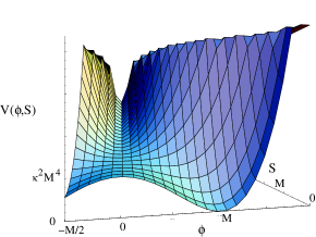
Figure 2: A representation of the potential for F-term inflation in the context of supersymmetry.

The potential, plotted in Fig. (2), has one valley of local minima, $V=\kappa^{2}M^{4}$, for $S>M$ with $\phi_{+}=\phi_{-}=0$, and one global supersymmetric minimum, $V=0$, at $S=0$ and $\phi_{+}=\phi_{-}=M$. Imposing initially $S\gg M$, the fields quickly settle down the valley of local minima. Since in the slow-roll inflationary valley the ground state of the scalar potential is non-zero, supersymmetry is broken. In the tree level, along the inflationary valley the potential is constant, therefore perfectly flat. A slope along the potential can be generated by including one-loop radiative corrections, which can be calculated using the Coleman-Weinberg expression cw

$$\Delta V_{1-{\rm loop}}=\frac{1}{64\pi^{2}}\sum_{i}(-1)^{F_{i}}m_{i}^{4}\ln\frac{m_{i}^{2}}{\Lambda^{2}}~{},$$ (4)

where the sum extends over all helicity states i, with fermion number $F_{i}$ and mass squared $m_{i}^{2}$; $\Lambda$ stands for a renormalisation scale. In this way, the scalar potential gets a little tilt which helps the inflaton field $S$ to slowly roll down the valley of minima. The one-loop radiative corrections to the scalar potential along the inflationary valley lead to the effective potential rs1

$$V_{\rm eff}^{\rm F}(|S|) = \kappa^{2}M^{4}\biggl{\{}1+\frac{\kappa^{2}\cal{N}}{32\pi^{2}}\biggl{[}2\ln\frac{|S|^{2}\kappa^{2}}{\Lambda^{2}}+(z+1)^{2}\ln(1+z^{-1})$$ (5)

$$~{}~{}~{}~{}~{}~{}~{}~{}~{}+(z-1)^{2}\ln(1-z^{-1})\biggr{]}\biggr{\}}~{}~{}\mbox{with}~{}~{}z=\frac{|S|^{2}}{M^{2}}~{};$$

$\cal{N}$ stands for the dimensionality of the representation to which the complex scalar components $\phi_{+},\phi_{-}$ of the chiral superfields $\Phi_{+},\Phi_{-}$ belong. This implies that the effective potential, Eq. (5), depends on the particular symmetry breaking scheme considered (see, Eq. (1)).

D-term Inflation

D-term inflation is one of the most interesting models of inflation. It is possible to implement it naturally within high energy physics, as for example Supersymmetric GUTS (SUSY GUTs), Supergravity (SUGRA), or string theories. Moreover, it avoids the Hubble-induced mass problem. In D-term inflation, the gauge symmetry is spontaneously broken by introducing Fayet-Iliopoulos (FI) D-terms. In standard D-term inflation, the constant FI term gets compensated by a single complex scalar field at the end of the inflationary era, which implies that standard D-term inflation ends with the formation of cosmic strings, called D-strings. More precisely, in its simplest form, the model requires a symmetry breaking scheme

$${\rm G}_{\rm GUT}\times{\rm U}(1)\stackrel{{\scriptstyle M_{\rm GUT}}}{{\hbox to22.76228pt{\rightarrowfill}}}{\rm H}\times{\rm U}(1)\,\lower 9.0pt\hbox{$\stackrel{{\scriptstyle\stackrel{{\scriptstyle\displaystyle M_{\rm infl}}}{{\hbox to28.45274pt{\rightarrowfill}}}}}{{\Phi_{+}\Phi_{-}}}$}\,{\rm H}\rightarrow{\rm G}_{\rm SM}~{}.$$ (6)

A supersymmetric description of the standard D-term inflation is insufficient; the inflaton field reaches values of the order of the Planck mass, or above it, even if one concentrates only around the last 60 e-folds of inflation; the correct analysis is therefore in the context of supergravity.

D-term inflation is based on the superpotential

$$W=\lambda S\Phi_{+}\Phi_{-}~{},$$ (7)

where $S,\Phi_{+},\Phi_{-}$ are three chiral superfields and $\lambda$ is the superpotential coupling. In its standard form, the model assumes an invariance under an Abelian gauge group $U(1)_{\xi}$, under which the superfields $S,\Phi_{+},\Phi_{-}$ have charges $0$, $+1$ and $-1$, respectively. It is also assumed the existence of a constant Fayet-Iliopoulos term $\xi$.

In the standard supergravity formulation the Lagrangian depends on the Kähler potential $K(\Phi_{i},\bar{\Phi}_{i})$ and the superpotential $W(\Phi_{i})$ only through the combination

$$G(\Phi_{i},\bar{\Phi}_{i})=\frac{K(\Phi_{i},\bar{\Phi}_{i})}{M_{\rm Pl}^{2}}+\ln\frac{|W(\Phi_{i})|^{2}}{M_{\rm Pl}^{6}}~{}.$$ (8)

However, this standard supergravity formulation is inappropriate to describe D-term inflation toine1 . In D-term inflation the superpotential vanishes at the unstable de Sitter vacuum (anywhere else the superpotential is nonzero). Thus, standard supergravity is inappropriate, since it is ill-defined at $W=0$. In conclusion, D-term inflation must be described with a non-singular formulation of supergravity when the superpotential vanishes.

Various formulations of effective supergravity can be constructed from the superconformal field theory. One must first build a Lagrangian with full superconformal theory, and then the gauge symmetries that are absent in Poincaré supergravity must be gauge fixed. In this way, one can construct a non-singular theory at $W=0$, where the action depends on all three functions: the Kähler potential $K(\Phi_{i},\bar{\Phi}_{i})$, the superpotential $W(\Phi_{i})$ and the kinetic function $f_{ab}(\Phi_{i})$ for the vector multiplets. To construct a formulation of supergravity with constant Fayet-Iliopoulos terms from superconformal theory, one finds toine1 that under U(1) gauge transformations in the directions in which there are constant Fayet-Iliopoulos terms $\xi_{\alpha}$, the superpotential $W$ must transform as toine1

$$\delta_{\alpha}W=\eta_{\alpha i}\partial^{i}W=-i\frac{g\xi_{\alpha}}{M_{\rm Pl}^{2}}W~{};$$ (9)

it is incorrect to keep the same charge assignments as in standard supergravity.

D-term inflationary models can be built with different choices of Kähler geometry. Let us first consider D-term inflation within minimal supergravity. It is based on

$$K_{\rm min}=\sum_{i}|\Phi_{i}|^{2}=|\Phi_{-}|^{2}+|\Phi_{+}|^{2}+|S|^{2}~{},$$ (10)

with $f_{ab}(\Phi_{i})=\delta_{ab}$. The tree level scalar potential is toine1

$$V_{\rm min}= \lambda^{2}\exp\left({\frac{|\phi_{-}|^{2}+|\phi_{+}|^{2}+|S|^{2}}{M^{2}_{\rm Pl}}}\right)\Biggl{[}|\phi_{+}\phi_{-}|^{2}\left(1+\frac{|S|^{4}}{M^{4}_{\rm Pl}}\right)$$ (11)

$$~{}~{}~{}~{}~{}~{}~{}~{}~{}~{}+|\phi_{+}S|^{2}\left(1+\frac{|\phi_{-}|^{4}}{M^{4}_{\rm Pl}}\right)+|\phi_{-}S|^{2}\left(1+\frac{|\phi_{+}|^{4}}{M^{4}_{\rm Pl}}\right)+3\frac{|\phi_{-}\phi_{+}S|^{2}}{M^{2}_{\rm Pl}}\Biggr{]}$$

$$+\ \frac{g^{2}}{2}\left(q_{+}|\phi_{+}|^{2}+q_{-}|\phi_{-}|^{2}+\xi\right)^{2}~{},$$

with

$$q_{\pm}=\pm 1-\xi/(2M_{\rm Pl}^{2})~{}.$$ (12)

The potential has two minima: One global minimum at zero and one local minimum equal to $V_{0}=(g^{2}/2)\xi^{2}$. For arbitrary large $S$ the tree level value of the potential remains constant and equal to $V_{0}$; the $S$ plays the rôle of the inflaton field. Assuming chaotic initial conditions $|S|\gg S_{\rm s}$, inflation begins. Along the inflationary trajectory the D-term, which is the dominant one, splits the masses in the $\Phi_{\pm}$ superfields, leading to the one-loop effective potential for the inflaton field. Considering the one-loop radiative corrections rs1 ; prl2005

$$V^{\rm eff}_{\rm min}(|S|)=\frac{g^{2}\xi^{2}}{2}\left\{1+\frac{g^{2}}{16\pi^{2}}\left[2\ln\left(z\frac{g^{2}\xi}{\Lambda^{2}}\right)+f_{V}(z)\right]\right\}~{},$$ (13)

where

$$f_{V}(z)=(z+1)^{2}\ln\left(1+\frac{1}{z}\right)+(z-1)^{2}\ln\left(1-\frac{1}{z}\right)~{},$$ (14)

with

$$z\equiv\frac{\lambda^{2}}{g^{2}\xi}|S|^{2}\exp\left(\frac{|S|^{2}}{M_{\rm Pl}^{2}}\right)~{}.$$ (15)

As a second example, consider D-term inflation based on Kähler geometry with a shift symmetry, $\phi\rightarrow\phi+c$ (where $c$ is a real constant). Such models can lead shift to flat enough potentials with stabilisation of the volume of the compactified space. They can therefore be used to built successful inflationary models in the framework of string theories. The Kähler potential is

$$K_{\rm shift}=\frac{1}{2}(S+\bar{S})^{2}+|\phi_{+}|^{2}+|\phi_{-}|^{2}~{};$$ (16)

the kinetic function has the minimal structure. The scalar potential reads rs3

$$V_{\rm shift} \simeq ~{}\frac{g^{2}}{2}\left(|\phi_{+}|^{2}-|\phi_{-}|^{2}+\xi\right)^{2}$$ (17)

$$+\lambda^{2}\exp\left({\frac{|\phi_{-}|^{2}+|\phi_{+}|^{2}}{M^{2}_{\rm Pl}}}\right)\exp\left[{\frac{(S+\bar{S})^{2}}{2M^{2}_{\rm Pl}}}\right]$$

$$~{}~{}~{}\times\Biggl{[}|\phi_{+}\phi_{-}|^{2}\left(1+\frac{S^{2}+\bar{S}^{2}}{M^{2}_{\rm Pl}}+\frac{|S|^{2}|S+\bar{S}|^{2}}{M^{4}_{\rm Pl}}\right)+|\phi_{+}S|^{2}\left(1+\frac{|\phi_{-}|^{4}}{M^{4}_{\rm Pl}}\right)$$

$$+|\phi_{-}S|^{2}\left(1+\frac{|\phi_{+}|^{4}}{M^{4}_{\rm Pl}}\right)+3\frac{|\phi_{-}\phi_{+}S|^{2}}{M^{2}_{\rm Pl}}\Biggr{]}~{}.$$

As in D-term inflation within minimal supergravity, the potential has a global minimum at zero for $\langle\Phi_{+}\rangle=0$ and $\langle\Phi_{-}\rangle=\sqrt{\xi}$ and a local minimum equal to $V_{0}=(g^{2}/2)\xi^{2}$ for $\langle S\rangle\gg S_{\rm c}$ and $\langle\Phi_{\pm}\rangle=0$.

The exponential factor $e^{|S|^{2}}$, which we got in the case of minimal supergravity, has been replaced by $e^{(S+\bar{S})^{2}/2}$. Writing $S=\eta+i\phi_{0}$ one gets $e^{(S+\bar{S})^{2}/2}=e^{\eta^{2}}$. If $\eta$ plays the rôle of the inflaton field, we obtain the same potential as for minimal D-term inflation. If instead $\phi_{0}$ is the inflaton field, the inflationary potential is identical to that of the usual D-term inflation within global supersymmetry rs1 . The latter case is better adapted with the choice $K_{\rm shift}$, since then the exponential term is constant during inflation and thus it cannot spoil the slow-roll conditions.

As a last example, consider a Kähler potential with non-renormalisable terms:

$$K_{\rm non-renorm} = |S|^{2}+|\Phi_{+}|^{2}+|\Phi_{-}|^{2}$$ (18)

$$+f_{+}\bigg{(}\frac{|S|^{2}}{M_{\rm Pl}^{2}}\bigg{)}|\Phi_{+}|^{2}+f_{-}\bigg{(}\frac{|S|^{2}}{M_{\rm Pl}^{2}}\bigg{)}|\Phi_{-}|^{2}+b\frac{|S|^{4}}{M_{\rm Pl}^{2}}~{},$$

where $f_{\pm}$ are arbitrary functions of $(|S|^{2}/M_{\rm Pl}^{2})$ and the superpotential is given in Eq. (7). The effective potential reads rs3

$$V^{\rm eff}_{\rm non-renorm}(|S|)=\frac{g^{2}\xi^{2}}{2}\left\{1+\frac{g^{2}}{16\pi^{2}}\left[2\ln\left(z\frac{g^{2}\xi}{\Lambda^{2}}\right)+f_{V}(z)\right]\right\}~{},$$ (19)

where

$$f_{V}(z)=(z+1)^{2}\ln\left(1+\frac{1}{z}\right)+(z-1)^{2}\ln\left(1-\frac{1}{z}\right)~{}$$ (20)

$$\mbox{with}~{}~{}~{}~{}z\equiv\frac{\lambda^{2}|S|^{2}}{g^{2}\xi}\exp\bigg{(}\frac{|S|^{2}}{M_{\rm Pl}^{2}}+b\frac{|S|^{4}}{M_{\rm Pl}^{4}}\bigg{)}\frac{1}{(1+f_{+})(1+f_{-})}~{}.$$ (21)

The cosmological consequences of these inflationary models will be presented in Section 5.

3 Topological Defects in GUTs

Following the standard version of the hot big bang model, the universe could have expanded from a very hot (with a temperature $T\hbox{ \raise 1.50696pt\hbox to0.0pt{$>$\hss}\lower 2.58334pt\hbox{$\sim$}\ }10^{19}{\rm GeV}$) and dense state, cooling towards its present state. As the universe expands and cools down, it undergoes a number of phase transitions, breaking the symmetry between the different interactions. Such phase transitions may leave behind topological defects  td as false vacuum remnants, via the Kibble mechanism kibble . Whether or not topological defects are formed during phase transitions followed by Spontaneously Broken Symmetries (SSB) depend on the topology of the vacuum manifold ${\cal M}_{n}$, which also determines the type of the produced defects. The properties of ${\cal M}_{n}$ are usually described by the $k^{\rm th}$ homotopy group $\pi_{k}({\cal M}_{n})$, which classifies distinct mappings from the $k$-dimensional sphere $S^{k}$ into the manifold ${\cal M}_{n}$.

Let me consider the symmetry breaking of a group G down to a subgroup H of G . If ${\cal M}_{n}={\rm G}/{\rm H}$ has disconnected components, or equivalently if the order $k$ of the nontrivial homotopy group is $k=0$, two-dimensional defects, domain walls, get formed. The spacetime dimension, $d$, of the defects is determined by the order of the nontrivial homotopy group by $d=4-1-k$. If ${\cal M}_{n}$ is not simply connected, meaning that ${\cal M}_{n}$ contains loops which cannot be continuously shrunk into a point, cosmic strings get produced. A necessary but not sufficient condition for the formation of stable strings is that the first (fundamental) homotopy group $\pi_{1}({\cal M}_{n})$ of ${\cal M}_{n}$, is nontrivial, or multiply connected. Cosmic strings are line-like $(d=2)$ defects. If ${\cal M}_{n}$ contains unshrinkable surfaces, then monopoles $(k=1,~{}d=1)$ get formed. Finally, if ${\cal M}_{n}$ contains non-contractible three-spheres, then event-like defects, called textures, $(k=3,~{}d=0)$ arise.

Depending on whether the original symmetry is local (gauged) or global (rigid), topological defects are called local or global. The energy of local defects is strongly confined, while the gradient energy of global defects is spread out over the causal horizon at defect formation. Patterns of symmetry breaking which lead to the formation of local monopoles or local domain walls are ruled out, since they should soon dominate the energy density of the universe and close it, unless an inflationary era took place after their formation. Local textures are insignificant in cosmology since their relative contribution to the energy density of the universe decreases rapidly with time textures .

Even if the non-trivial topology required for the existence of a defect is absent in a field theory, it may still be possible to have defect-like solutions. Defects may be embedded in such topologically trivial field theories embedded . While stability of topological defects is guaranteed by topology, embedded defects are in general unstable under small perturbations.

3.1 Cosmic Strings

Cosmic strings mslnp are analogous to flux tubes in type-II superconductors, or to vortex filaments in superfluid helium. Topologically stable strings do not have ends; they either form closed loops or they extend to infinity. The linear mass density of strings, $\mu$, which in the simplest models it also determines the string tension, specifies the energy scale, $\eta$, of the symmetry breaking, $\mu\sim\eta^{2}$. The strength of gravitational interactions of strings is expressed in terms of the dimensionless parameter $G\mu\sim\eta^{2}/M_{\rm Pl}^{2}$ (with $G$ the gravitational Newton’s constant and $M_{\rm Pl}$ the Planck mass). For grand unification strings, the energy per unit length is $\mu\sim 10^{22}{\rm kg}/{\rm m}$, or equivalently, $G\mu\sim{\cal O}(10^{-6})$.

At formation, cosmic strings form a tangled network, made of Brownian infinitely long strings and a distribution of closed loops. Curved segments of strings moving under their tension reach almost relativistic speeds. When two string segments intersect, they exchange partners (intercommute) with probability equal to 1. String-string and self-string intersections lead to daughter infinitely long strings and closed loops, as they can be seen in Fig. (3).

Figure 3: At the top, string-string interactions at one point leading to the formation of two new long strings via exchange of partners. In the middle, string-string interactions at two points, leading to two new long strings and a loop. At the bottom, self-self interactions leading to the formation of a new long string and a loop mslnp .

Clearly, string intercommutations produce discontinuities on the new string segments at the intersection point. These discontinuities (kinks) are composed of right- and left-moving pieces travelling along the string at the speed of light.

Early analytic work one-scale identified the key property of scaling, where at least the basic properties of the string network can be characterised by a single length scale, roughly the persistence length (defined as the distance beyond which the directions along the string are uncorrelated), $\xi(t)$, and the typical separation between string segments, $d(t)$, both grow with the cosmic horizon. This result was supported by subsequent numerical work numcs . However, further investigation revealed dynamical processes, including loop production, at scales much smaller than $\xi$ proc .

Recent numerical simulations of cosmic string evolution in a expanding universe found evidence cmf of a scaling regime for the cosmic string loops in the radiation and matter dominated eras down to the hundredth of the horizon time. It is important to note that the scaling was found without considering any gravitational back reaction effect; it was just the result of string intercommuting mechanism. As it was reported in Ref. cmf , the scaling regime of string loops appears after a transient relaxation era, driven by a transient overproduction of string loops with lengths close to the initial correlation length of the string network. Calculating the amount of energy momentum tensor lost from the string network, it was found cmf that a few percents of the total string energy density disappear in the very brief process of formation of numerically unresolved string loops during the very first timesteps of the string evolution. Subsequently, other studies supported these findings vov . A snapshot of the evolution of a cosmic string network during the matter dominated era is shown in Fig. 4.

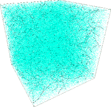
Figure 4: Snapshot of a string network in the matter-dominated era cmf .

3.2 Genericity of Cosmic String Formation within SUSY GUTs

To investigate the cosmological consequences of cosmic strings formed at the end of hybrid inflation, one should first address the question of whether such objects are generically formed. I will briefly discuss the genericity of cosmic string formation in the framework of SUSY GUTS.

Even though the Standard Model has been tested to a very high precision, it is incapable of explaining neutrino masses SK . An extension of the Standard Model gauge group can be realised within Supersymmetry (SUSY). SUSY offers a solution to the gauge hierarchy problem, while in the supersymmetric standard model the gauge coupling constants of the strong, weak and electromagnetic interactions meet at a single point $M_{\rm GUT}\simeq(2-3)\times 10^{16}$ GeV. In addition, SUSY GUTs can provide the scalar field which could drive inflation, explain the matter-antimatter asymmetry of the universe, and propose a candidate, the lightest superparticle, for cold dark matter.

Within SUSY GUTs there is a large number of SSB patterns leading from a large gauge group G to the SM gauge group G${}_{\rm SM}\equiv$ SU(3)${}_{\rm C}\times$ SU(2)${}_{\rm L}\times$ U(1)_Y. The study of the homotopy group of the false vacuum for each SSB scheme will determine whether there is defect formation and it will identify the type of the formed defect. Clearly, if there is formation of domain walls or monopoles, one will have to place an era of supersymmetric hybrid inflation to dilute them. To consider a SSB scheme as a successful one, it should be able to explain the matter/anti-matter asymmetry of the universe and to account for the proton lifetime measurements SK . In what follows, I consider a mechanism of baryogenesis via leptogenesis, which can be thermal or non-thermal one. In the case of non-thermal leptogenesis, U(1)_B-L (B and L, are the baryon and lepton numbers, respectively) is a sub-group of the GUT gauge group, G_GUT, and B-L is broken at the end or after inflation. In the case of thermal leptogenesis, B-L is broken independently of inflation. If leptogenesis is thermal and B-L is broken before the inflationary era, then one should check whether the temperature at which B-L is broken, which will define the mass of the right-handed neutrinos, is smaller than the reheating temperature which should be lower than the limit imposed by the gravitino. To ensure the stability of proton, the discrete symmetry Z₂, which is contained in U(1)_B-L, must be kept unbroken down to low energies. This implies that the successful SSB schemes should end at G${}_{\rm SM}\times$ Z₂. I will then examine how often cosmic strings have survived after the inflationary era, within all acceptable SSB patterns.

To accomplish this task one has to choose the large gauge group G_GUT. In Ref. jrs this study has been done explicitly for a large number of simple Lie groups. Since I consider GUTs based on simple gauge groups, the type of supersymmetric hybrid inflation will be of the F-type. The minimum rank of G_GUT has to be at least equal to 4, to contain the G_SM as a subgroup. Then one has to study the possible embeddings of G_SM in G_GUT to be in agreement with the Standard Model phenomenology and especially with the hypercharges of the known particles. Moreover, the group must include a complex representation, needed to describe the Standard Model fermions, and it must be anomaly free. Since, in principle, ${\rm SU}(n)$ may not be anomaly free, I assume that the ${\rm SU}(n)$ groups which I use, they have indeed a fermionic representation that certifies that the model is anomaly free. I set as the upper bound on the rank $r$ of the group, $r\leq 8$. Clearly, the choice of the maximum rank is in principle arbitrary. This choice could, in a sense, be motivated by the Horava-Witten hw model, based on ${\rm E}_{8}\times{\rm E}_{8}$. Thus, the large gauge group G_GUT could be one of the following: SO(10), E₆, SO(14), SU(8), SU(9); flipped SU(5) and [SU(3)]³ are included within this list as subgroups of SO(10) and E₆, respectively.

A detailed study of all the SSB schemes which bring us from G_GUT down to the Standard Model gauge group G_SM, by one or more intermediate steps, shows that cosmic strings are generically formed at the end of hybrid inflation. If the large gauge group G_GUT is SO(10) then cosmic strings formation is unavoidable jrs ; rachel . For ${\rm E}_{6}$ it depends whether one considers thermal or non-thermal leptogenesis. More precisely, under the assumption of non-thermal leptogenesis then cosmic strings formation is unavoidable. If I consider thermal leptogenesis then cosmic strings formation at the end of hybrid inflation arises in $98\%$ of the acceptable SSB schemes jm . If the requirement of having Z₂ unbroken down to low energies is relaxed and thermal leptogenesis is considered as being the mechanism for baryogenesis, then cosmic strings formation accompanies hybrid inflation in $80\%$ of the SSB schemes jm .

For an illustration I give below the list of the SSB schemes of ${\rm E}_{6}$ down to the G${}_{\rm SM}\times Z_{2}$ via ${\rm SO}(10)\times{\rm U}(1)$ (the reader is referred to Ref. jrs for a full analysis). Every $\stackrel{{\scriptstyle n}}{{\longrightarrow}}$ represent an SSB during which there is formation of topological defects, whose type is denoted by $n$: $1$ for monopoles, $2$ for topological cosmic strings, $2^{\prime}$ for embedded strings, $3$ for domain walls. Note that for e.g. $3_{\rm C}~{}2_{\rm L}~{}2_{\rm R}~{}1_{\rm B-L}$ stands for SU(3)${}_{\rm C}\times$ SU(2)${}_{\rm L}\times$ SU(2) ${}_{\rm R}\times$ U(1)_B-L.

$${\begin{array}[]{cllllll}{\rm E}_{6}\stackrel{{\scriptstyle 1}}{{\rightarrow}}{\rm SO(10)}~{}1_{\rm V^{\prime}}&\left\{\begin{array}[]{cllllccccc}\stackrel{{\scriptstyle 2}}{{\longrightarrow}}&{\rm SO(10)}&\stackrel{{\scriptstyle}}{{\longrightarrow}}~{}~{}~{}\mbox{{\rm Eq.~{}(\ref{eq:51})}}\\ \stackrel{{\scriptstyle 1}}{{\longrightarrow}}&5~{}1_{\rm V}~{}1_{\rm V^{\prime}}&\stackrel{{\scriptstyle}}{{\longrightarrow}}~{}~{}~{}\mbox{{\rm Eq.~{}(\ref{eq:5})}}\\ \stackrel{{\scriptstyle 1}}{{\longrightarrow}}&5_{\rm F}~{}1_{\rm V}~{}1_{\rm V^{\prime}}&\stackrel{{\scriptstyle}}{{\longrightarrow}}~{}~{}~{}\mbox{{\rm Eq.~{}(\ref{eq:5F})}}\\ \stackrel{{\scriptstyle 1}}{{\longrightarrow}}&5_{\rm E}~{}1_{\rm V}~{}1_{\rm V^{\prime}}&\stackrel{{\scriptstyle 2^{\prime},2}}{{\longrightarrow}}~{}~{}{\rm G}_{\rm SM}~{}Z_{2}\\ \stackrel{{\scriptstyle 2}}{{\longrightarrow}}&5~{}1_{\rm V^{\prime}}~{}Z_{2}&\stackrel{{\scriptstyle}}{{\longrightarrow}}~{}~{}~{}\mbox{{\rm Eq.~{}(\ref{eq:5}a)}}\\ \stackrel{{\scriptstyle 1,2}}{{\longrightarrow}}&5~{}1_{\rm V}&\stackrel{{\scriptstyle}}{{\longrightarrow}}~{}~{}~{}\mbox{{\rm Eq.~{}(\ref{eq:51}a)}}\\ \stackrel{{\scriptstyle 1}}{{\longrightarrow}}&5_{\rm F}~{}1_{\rm V}&\stackrel{{\scriptstyle 2^{\prime},2}}{{\longrightarrow}}~{}~{}{\rm G}_{\rm SM}~{}Z_{2}\\ \stackrel{{\scriptstyle 1}}{{\longrightarrow}}&{\rm G}_{\rm SM}~{}1_{\rm V}&\stackrel{{\scriptstyle 2}}{{\longrightarrow}}~{}~{}{\rm G}_{\rm SM}~{}Z_{2}\\ \stackrel{{\scriptstyle 1,2}}{{\longrightarrow}}&{\rm G}_{\rm SM}~{}1_{\rm V^{\prime}}~{}Z_{2}&\stackrel{{\scriptstyle 2}}{{\longrightarrow}}~{}~{}{\rm G}_{\rm SM}~{}Z_{2}\\ \stackrel{{\scriptstyle 1,2}}{{\longrightarrow}}&4_{\rm C}~{}2_{\rm L}~{}2_{\rm R}~{}1_{\rm V^{\prime}}&\stackrel{{\scriptstyle}}{{\longrightarrow}}~{}~{}~{}\mbox{{\rm Eq.~{}(\ref{eq:ps6})}}\\ \stackrel{{\scriptstyle 1}}{{\longrightarrow}}&4_{\rm C}~{}2_{\rm L}~{}2_{\rm R}&\stackrel{{\scriptstyle}}{{\longrightarrow}}~{}~{}~{}\mbox{{\rm Eq. (\ref{eq:ps})}}\\ \stackrel{{\scriptstyle 1}}{{\longrightarrow}}&3_{\rm C}~{}2_{\rm L}~{}2_{\rm R}~{}1_{\rm B-L}~{}1_{\rm V^{\prime}}&\stackrel{{\scriptstyle}}{{\longrightarrow}}~{}~{}~{}\mbox{{\rm Eq.~{}(\ref{eq:ps6}c)}}\\ \stackrel{{\scriptstyle 1}}{{\longrightarrow}}&3_{\rm C}~{}2_{\rm L}~{}1_{\rm R}~{}1_{\rm B-L}~{}1_{\rm V^{\prime}}&\stackrel{{\scriptstyle}}{{\longrightarrow}}~{}~{}~{}\mbox{{\rm Eq.~{}(\ref{eq:ps6}b)}}\\ \end{array}\right.\end{array}}$$ (22)

where

$${{\rm SO(10)}\left\{\begin{array}[]{cccccc}\stackrel{{\scriptstyle 1}}{{\longrightarrow}}&5~{}1_{\rm V}&\stackrel{{\scriptstyle 1}}{{\longrightarrow}}&3_{\rm C}~{}2_{\rm L}~{}1_{\rm Z}~{}1_{\rm V}&\stackrel{{\scriptstyle 2}}{{\longrightarrow}}&{\rm G}_{\rm SM}~{}Z_{2}\\ \stackrel{{\scriptstyle 1}}{{\longrightarrow}}&4_{\rm C}~{}2_{\rm L}~{}2_{\rm R}&\stackrel{{\scriptstyle}}{{\longrightarrow}}&\mbox{\rm Eq. (\ref{eq:ps})}\\ \stackrel{{\scriptstyle 1,2}}{{\longrightarrow}}&4_{\rm C}~{}2_{\rm L}~{}2_{\rm R}~{}Z_{2}^{\rm C}&\stackrel{{\scriptstyle}}{{\longrightarrow}}&\mbox{{\rm Eq. (\ref{eq:psZ2})}}\\ \stackrel{{\scriptstyle 1,2}}{{\longrightarrow}}&4_{\rm C}~{}2_{\rm L}~{}1_{\rm R}~{}Z_{2}^{\rm C}&\stackrel{{\scriptstyle}}{{\longrightarrow}}&\mbox{{\rm Eq. (\ref{eq:psZ2}b)}}\\ \stackrel{{\scriptstyle 1}}{{\longrightarrow}}&4_{\rm C}~{}2_{\rm L}~{}1_{\rm R}&\stackrel{{\scriptstyle}}{{\longrightarrow}}&\mbox{\rm Eq. (\ref{eq:ps}b)}\\ \stackrel{{\scriptstyle 1,2}}{{\longrightarrow}}&3_{\rm C}~{}2_{\rm L}~{}2_{\rm R}~{}1_{\rm B-L}~{}Z_{2}^{\rm C}&\stackrel{{\scriptstyle}}{{\longrightarrow}}&\mbox{{\rm Eq. (\ref{eq:psZ2}a)}}\\ \stackrel{{\scriptstyle 1}}{{\longrightarrow}}&3_{\rm C}~{}2_{\rm L}~{}2_{\rm R}~{}1_{\rm B-L}&\stackrel{{\scriptstyle}}{{\longrightarrow}}&\mbox{{\rm Eq. (\ref{eq:ps}a)}}\\ \stackrel{{\scriptstyle 1}}{{\longrightarrow}}&3_{\rm C}~{}2_{\rm L}~{}1_{\rm R}~{}1_{\rm B-L}&\stackrel{{\scriptstyle 2}}{{\longrightarrow}}&{\rm G}_{\rm SM}~{}Z_{2}\\ \end{array}\right.}$$ (23)

$$\begin{array}[]{clllllccc}5~{}1_{\rm V}~{}1_{\rm V^{\prime}}&\left\{\begin{array}[]{clllllccc}\stackrel{{\scriptstyle 2}}{{\longrightarrow}}&5~{}1_{\rm V^{\prime}}~{}Z_{2}&\left\{\begin{array}[]{clllllccc}\stackrel{{\scriptstyle 1}}{{\longrightarrow}}&{\rm G}_{\rm SM}~{}1_{\rm V^{\prime}}~{}Z_{2}&\stackrel{{\scriptstyle 2}}{{\longrightarrow}}&{\rm G}_{\rm SM}~{}Z_{2}\\ \end{array}\right.\\ \stackrel{{\scriptstyle 1}}{{\longrightarrow}}&{\rm G}_{\rm SM}~{}1_{\rm V}~{}1_{\rm V^{\prime}}&\left\{\begin{array}[]{cllllllccc}\stackrel{{\scriptstyle 2}}{{\longrightarrow}}&{\rm G}_{\rm SM}~{}1_{\rm V}&\stackrel{{\scriptstyle 2}}{{\longrightarrow}}&{\rm G}_{\rm SM}~{}Z_{2}\\ \stackrel{{\scriptstyle 2}}{{\longrightarrow}}&{\rm G}_{\rm SM}~{}1_{\rm V^{\prime}}~{}Z_{2}&\stackrel{{\scriptstyle 2}}{{\longrightarrow}}&{\rm G}_{\rm SM}~{}Z_{2}\\ \end{array}\right.\\ \stackrel{{\scriptstyle 2}}{{\longrightarrow}}&5~{}1_{\rm V}&\stackrel{{\scriptstyle}}{{\longrightarrow}}~{}~{}~{}\mbox{{\rm Eq.~{}(\ref{eq:51}a)}}\\ \end{array}\right.\end{array}$$ (24)

$$\begin{array}[]{clllllccc}5_{\rm F}~{}1_{\rm V}~{}1_{\rm V^{\prime}}&\left\{\begin{array}[]{cllllccc}~{}\stackrel{{\scriptstyle 2}}{{\longrightarrow}}&~{}~{}5_{\rm F}~{}1_{\rm V}&\stackrel{{\scriptstyle 2^{\prime},2}}{{\longrightarrow}}&{\rm G}_{\rm SM}~{}Z_{2}\\ ~{}\stackrel{{\scriptstyle 2^{\prime},2}}{{\longrightarrow}}&~{}{\rm G}_{\rm SM}~{}Z_{2}\\ \end{array}\right.\end{array}$$ (25)

$$\begin{array}[]{clllllccc}4_{\rm C}~{}2_{\rm L}~{}2_{\rm R}~{}1_{\rm V^{\prime}}&\left\{\begin{array}[]{cllllccc}\stackrel{{\scriptstyle 2}}{{\longrightarrow}}&4_{\rm C}~{}2_{\rm L}~{}2_{\rm R}&\stackrel{{\scriptstyle}}{{\longrightarrow}}~{}~{}~{}\mbox{{\rm Eq.~{}(\ref{eq:ps})}}\\ \stackrel{{\scriptstyle 1}}{{\longrightarrow}}&3_{\rm C}~{}2_{\rm L}~{}1_{\rm R}~{}1_{\rm B-L}~{}1_{\rm V^{\prime}}&\left\{\begin{array}[]{cllllllccc}\stackrel{{\scriptstyle 2}}{{\longrightarrow}}&3_{\rm C}~{}2_{\rm L}~{}1_{\rm R}~{}1_{\rm B-L}&\stackrel{{\scriptstyle 2}}{{\longrightarrow}}&{\rm G}_{\rm SM}~{}Z_{2}\\ \stackrel{{\scriptstyle 2^{\prime},2}}{{\longrightarrow}}&{\rm G}_{\rm SM}1_{\rm V^{\prime}}~{}Z_{2}&\stackrel{{\scriptstyle 2}}{{\longrightarrow}}&{\rm G}_{\rm SM}~{}Z_{2}\\ \stackrel{{\scriptstyle 2^{\prime},2}}{{\longrightarrow}}&{\rm G}_{\rm SM}~{}Z_{2}\\ \end{array}\right.\\ \stackrel{{\scriptstyle 1}}{{\longrightarrow}}&3_{\rm C}~{}2_{\rm L}~{}2_{\rm R}~{}1_{\rm B-L}~{}1_{\rm V^{\prime}}&\left\{\begin{array}[]{cllllccc}\stackrel{{\scriptstyle 1}}{{\longrightarrow}}&3_{\rm C}~{}2_{\rm L}~{}1_{\rm R}~{}1_{\rm B-L}~{}1_{\rm V^{\prime}}&\stackrel{{\scriptstyle}}{{\longrightarrow}}~{}~{}~{}\mbox{{\rm Eq.~{}(\ref{eq:ps6}b)}}\\ \stackrel{{\scriptstyle 2}}{{\longrightarrow}}&3_{\rm C}~{}2_{\rm L}~{}2_{\rm R}~{}1_{\rm B-L}&\stackrel{{\scriptstyle}}{{\longrightarrow}}~{}~{}~{}\mbox{{\rm Eq.~{}(\ref{eq:ps}a)}}\\ \stackrel{{\scriptstyle 2^{\prime},2}}{{\longrightarrow}}&{\rm G}_{\rm SM}1_{\rm V^{\prime}}~{}Z_{2}&\stackrel{{\scriptstyle 2}}{{\longrightarrow}}~{}~{}~{}{\rm G}_{\rm SM}~{}Z_{2}\\ \stackrel{{\scriptstyle 1,2}}{{\longrightarrow}}&3_{\rm C}~{}2_{\rm L}~{}1_{\rm R}~{}1_{\rm B-L}&\stackrel{{\scriptstyle 2}}{{\longrightarrow}}~{}~{}~{}{\rm G}_{\rm SM}~{}Z_{2}\\ \stackrel{{\scriptstyle 2^{\prime},2}}{{\longrightarrow}}&{\rm G}_{\rm SM}~{}Z_{2}\\ \end{array}\right.\\ \stackrel{{\scriptstyle 1}}{{\longrightarrow}}&4_{\rm C}~{}2_{\rm L}~{}1_{\rm R}~{}1_{\rm V^{\prime}}&\left\{\begin{array}[]{cllllccc}\stackrel{{\scriptstyle 2}}{{\longrightarrow}}&4_{\rm C}~{}2_{\rm L}~{}1_{\rm R}&\stackrel{{\scriptstyle}}{{\longrightarrow}}&~{}~{}~{}\mbox{{\rm Eq.~{}(\ref{eq:ps}b)}}\\ \stackrel{{\scriptstyle 1}}{{\longrightarrow}}&3_{\rm C}~{}2_{\rm L}~{}1_{\rm R}~{}1_{\rm B-L}~{}1_{\rm V^{\prime}}&\stackrel{{\scriptstyle}}{{\longrightarrow}}&~{}~{}~{}\mbox{{\rm Eq.~{}(\ref{eq:ps6}b)}}\\ \stackrel{{\scriptstyle 2^{\prime},2}}{{\longrightarrow}}&{\rm G}_{\rm SM}1_{\rm V^{\prime}}~{}Z_{2}&\stackrel{{\scriptstyle 2}}{{\longrightarrow}}&{\rm G}_{\rm SM}~{}Z_{2}\\ \stackrel{{\scriptstyle 1,2}}{{\longrightarrow}}&3_{\rm C}~{}2_{\rm L}~{}1_{\rm R}~{}1_{\rm B-L}&\stackrel{{\scriptstyle 2}}{{\longrightarrow}}&{\rm G}_{\rm SM}~{}Z_{2}\\ \stackrel{{\scriptstyle 2}}{{\longrightarrow}}&{\rm G}_{\rm SM}~{}Z_{2}\\ \end{array}\right.\\ \stackrel{{\scriptstyle 1,2}}{{\longrightarrow}}&{\rm G}_{\rm SM}1_{\rm V^{\prime}}~{}Z_{2}&\stackrel{{\scriptstyle 2}}{{\longrightarrow}}~{}~{}~{}{\rm G}_{\rm SM}~{}Z_{2}\\ \stackrel{{\scriptstyle 1,2}}{{\longrightarrow}}&3_{\rm C}~{}2_{\rm L}~{}2_{\rm R}~{}1_{\rm B-L}&\stackrel{{\scriptstyle}}{{\longrightarrow}}~{}~{}~{}\mbox{{\rm Eq.~{}(\ref{eq:ps}a)}}\\ \stackrel{{\scriptstyle 1}}{{\longrightarrow}}&3_{\rm C}~{}2_{\rm L}~{}1_{\rm R}~{}1_{\rm B-L}&\stackrel{{\scriptstyle 2}}{{\longrightarrow}}~{}~{}~{}{\rm G}_{\rm SM}~{}Z_{2}\\ \end{array}\right.\end{array}$$ (26)

with

$$\begin{array}[]{clllcccc}4_{\rm C}~{}2_{\rm L}~{}2_{\rm R}&\left\{\begin{array}[]{cllllccc}\stackrel{{\scriptstyle 1}}{{\longrightarrow}}&3_{\rm C}~{}2_{\rm L}~{}2_{\rm R}~{}1_{\rm B-L}&\left\{\begin{array}[]{cllllccc}\stackrel{{\scriptstyle 1}}{{\longrightarrow}}&3_{\rm C}~{}2_{\rm L}~{}1_{\rm R}~{}1_{\rm B-L}&\stackrel{{\scriptstyle 2}}{{\longrightarrow}}&{\rm G}_{\rm SM}~{}Z_{2}\\ \stackrel{{\scriptstyle 2^{\prime},2}}{{\longrightarrow}}&{\rm G}_{\rm SM}~{}Z_{2}\\ \end{array}\right.\\ \stackrel{{\scriptstyle 1}}{{\longrightarrow}}&4_{\rm C}~{}2_{\rm L}~{}1_{\rm R}&\left\{\begin{array}[]{cllllccc}\stackrel{{\scriptstyle 1}}{{\longrightarrow}}&3_{\rm C}~{}2_{\rm L}~{}1_{\rm R}~{}1_{\rm B-L}&\stackrel{{\scriptstyle 2}}{{\longrightarrow}}&{\rm G}_{\rm SM}~{}Z_{2}\\ \stackrel{{\scriptstyle 2^{\prime},2}}{{\longrightarrow}}&{\rm G}_{\rm SM}~{}Z_{2}\\ \end{array}\right.\\ \stackrel{{\scriptstyle 1}}{{\longrightarrow}}&3_{\rm C}~{}2_{\rm L}~{}1_{\rm R}~{}1_{\rm B-L}&~{}~{}~{}~{}\stackrel{{\scriptstyle 2}}{{\longrightarrow}}~{}~{}{\rm G}_{\rm SM}~{}Z_{2}\\ \end{array}\right.\end{array}$$ (27)

$$\begin{array}[]{clllcccc}4_{\rm C}~{}2_{\rm L}~{}2_{\rm R}~{}Z_{2}^{\rm C}&\left\{\begin{array}[]{cllllccc}\stackrel{{\scriptstyle 1}}{{\longrightarrow}}&3_{\rm C}~{}2_{\rm L}~{}2_{\rm R}~{}1_{\rm B-L}~{}Z_{2}^{\rm C}&\left\{\begin{array}[]{cllllccc}\stackrel{{\scriptstyle 3}}{{\longrightarrow}}&3_{\rm C}~{}2_{\rm L}~{}2_{\rm R}~{}1_{\rm B-L}&\stackrel{{\scriptstyle}}{{\longrightarrow}}&~{}~{}~{}\mbox{\rm Eq. (\ref{eq:ps}a)}\\ \stackrel{{\scriptstyle 1,3}}{{\longrightarrow}}&3_{\rm C}~{}2_{\rm L}~{}1_{\rm R}~{}1_{\rm B-L}&\stackrel{{\scriptstyle 2}}{{\longrightarrow}}&{\rm G}_{\rm SM}~{}Z_{2}\\ \end{array}\right.\\ \stackrel{{\scriptstyle 1}}{{\longrightarrow}}&4_{\rm C}~{}2_{\rm L}~{}1_{\rm R}~{}Z_{2}^{\rm C}&\left\{\begin{array}[]{cllllccc}\stackrel{{\scriptstyle 3}}{{\longrightarrow}}&4_{\rm C}~{}2_{\rm L}~{}1_{\rm R}&{\longrightarrow}&~{}~{}~{}\mbox{\rm Eq. (\ref{eq:ps}b)}\\ \stackrel{{\scriptstyle 1,3}}{{\longrightarrow}}&3_{\rm C}~{}2_{\rm L}~{}1_{\rm R}~{}1_{\rm B-L}&\stackrel{{\scriptstyle 2}}{{\longrightarrow}}&{\rm G}_{\rm SM}~{}Z_{2}\\ \end{array}\right.\\ \stackrel{{\scriptstyle 3}}{{\longrightarrow}}&4_{\rm C}~{}2_{\rm L}~{}2_{\rm R}&{\longrightarrow}~{}~{}~{}\mbox{\rm Eq. (\ref{eq:ps})}\\ \stackrel{{\scriptstyle 1}}{{\longrightarrow}}&4_{\rm C}~{}2_{\rm L}~{}1_{\rm R}&{\longrightarrow}~{}~{}~{}\mbox{\rm Eq. (\ref{eq:ps}b)}\\ \stackrel{{\scriptstyle 1,3}}{{\longrightarrow}}&3_{\rm C}~{}2_{\rm L}~{}2_{\rm R}~{}1_{\rm B-L}&\stackrel{{\scriptstyle}}{{\longrightarrow}}~{}~{}~{}~{}\mbox{\rm Eq. (\ref{eq:ps}a)}\\ \stackrel{{\scriptstyle 1,3}}{{\longrightarrow}}&3_{\rm C}~{}2_{\rm L}~{}1_{\rm R}~{}1_{\rm B-L}&\stackrel{{\scriptstyle 2}}{{\longrightarrow}}~{}~{}~{}{\rm G}_{\rm SM}~{}Z_{2}\end{array}\right.\end{array}$$ (28)

In addition, there are more direct schemes; they are listed below:

$${{\rm E}_{6}\left\{\begin{array}[]{clllllcccc}&\stackrel{{\scriptstyle 1}}{{\longrightarrow}}&5~{}1_{\rm V}~{}1_{\rm V^{\prime}}&\stackrel{{\scriptstyle}}{{\longrightarrow}}&\mbox{{\rm Eq.(\ref{eq:5})}}\\ &\stackrel{{\scriptstyle 1}}{{\longrightarrow}}&5_{\rm F}~{}1_{\rm V}~{}1_{\rm V^{\prime}}&\stackrel{{\scriptstyle}}{{\longrightarrow}}&\mbox{{\rm Eq.(\ref{eq:5F})}}\\ &\stackrel{{\scriptstyle 1}}{{\longrightarrow}}&5_{\rm E}~{}1_{\rm V}~{}1_{\rm V^{\prime}}&\stackrel{{\scriptstyle 2^{\prime},2}}{{\longrightarrow}}&{\rm G}_{\rm SM}~{}Z_{2}\\ &\stackrel{{\scriptstyle 1}}{{\longrightarrow}}&5~{}1_{\rm V}&\stackrel{{\scriptstyle}}{{\longrightarrow}}&\mbox{{\rm Eq.(\ref{eq:51}a)}}\\ &\stackrel{{\scriptstyle 1}}{{\longrightarrow}}&5~{}1_{\rm V^{\prime}}&\stackrel{{\scriptstyle}}{{\longrightarrow}}&\mbox{{\rm Eq.(\ref{eq:5}a)}}\\ &\stackrel{{\scriptstyle 1}}{{\longrightarrow}}&5_{\rm F}~{}1_{\rm V}&\stackrel{{\scriptstyle 2^{\prime},2}}{{\longrightarrow}}&{\rm G}_{\rm SM}~{}Z_{2}\\ &\stackrel{{\scriptstyle 1}}{{\longrightarrow}}&4_{\rm C}~{}2_{\rm L}~{}2_{\rm R}~{}1_{\rm V^{\prime}}&\stackrel{{\scriptstyle}}{{\longrightarrow}}&\mbox{\rm Eq. (\ref{eq:ps6})}\\ &\stackrel{{\scriptstyle 1}}{{\longrightarrow}}&4_{\rm C}~{}2_{\rm L}~{}2_{\rm R}&\stackrel{{\scriptstyle}}{{\longrightarrow}}&\mbox{{\rm Eq.~{}(\ref{eq:ps})}}\\ &\stackrel{{\scriptstyle 1}}{{\longrightarrow}}&4_{\rm C}~{}2_{\rm L}~{}1_{\rm R}&\stackrel{{\scriptstyle}}{{\longrightarrow}}&\mbox{{\rm Eq.~{}(\ref{eq:ps}b)}}\\ &\stackrel{{\scriptstyle 1}}{{\longrightarrow}}&4_{\rm C}~{}2_{\rm L}~{}1_{\rm R}~{}1_{\rm V^{\prime}}&\stackrel{{\scriptstyle}}{{\longrightarrow}}&\mbox{{\rm Eq.~{}(\ref{eq:ps6}d)}}\\ &\stackrel{{\scriptstyle 1}}{{\longrightarrow}}&3_{\rm C}~{}2_{\rm L}~{}2_{\rm R}~{}1_{\rm B-L}~{}1_{\rm V^{\prime}}&\stackrel{{\scriptstyle}}{{\longrightarrow}}&\mbox{{\rm Eq.~{}(\ref{eq:ps6}c)}}\\ &\stackrel{{\scriptstyle 1}}{{\longrightarrow}}&3_{\rm C}~{}2_{\rm L}~{}1_{\rm R}~{}1_{\rm B-L}~{}1_{\rm V^{\prime}}&\stackrel{{\scriptstyle}}{{\longrightarrow}}&\mbox{{\rm Eq.~{}(\ref{eq:ps6}b)}}\\ &\stackrel{{\scriptstyle 1}}{{\longrightarrow}}&3_{\rm C}~{}2_{\rm L}~{}1_{\rm R}~{}1_{\rm B-L}&\stackrel{{\scriptstyle 2}}{{\longrightarrow}}&{\rm G}_{\rm SM}~{}Z_{2}\\ &\stackrel{{\scriptstyle 1}}{{\longrightarrow}}&{\rm G}_{\rm SM}~{}1_{\rm V}&\stackrel{{\scriptstyle 2}}{{\longrightarrow}}&{\rm G}_{\rm SM}~{}Z_{2}\\ &\stackrel{{\scriptstyle 1,2}}{{\longrightarrow}}&{\rm G}_{\rm SM}~{}1_{\rm V^{\prime}}~{}Z_{2}&\stackrel{{\scriptstyle 2}}{{\longrightarrow}}&{\rm G}_{\rm SM}~{}Z_{2}\\ \end{array}\right.}$$ (29)

The SSB schemes of SU(6) and SU(7) down to the G_SM which could accommodate an inflationary era with no defect (of any kind) at later times are inconsistent with proton lifetime measurements and minimal SU(6) and SU(7) do not predict neutrino masses jrs , implying that these models are incompatible with high energy physics phenomenology. Higher rank groups, namely SO(14), SU(8) and SU(9), should in general lead to cosmic string formation at the end of hybrid inflation. In all these schemes, cosmic string formation is sometimes accompanied by the formation of embedded strings. The strings which form at the end of hybrid inflation have a mass which is proportional to the inflationary scale.

4 Braneworld Cosmology

One of our dreams in theoretical physics is to be able to unify all fundamental interactions into a unique theory. String theory offers one such attempt to unify gravity with the other interactions, in a self-consistent quantum theory. String theory is based on the proposal that one-dimensional extended objects (strings) are the fundamental constituents of matter. In the mid 1990’s it was realised that higher dimensional extended membranes ($p$-branes, with $p>1$) should also play a crucial rôle in string theory. In particular, branes offer the possibility of relating apparently different string theories. Of particular importance among $p$-branes are the $Dp$-branes on which open strings can end; they can describe matter fields living on the brane. Closed strings (eg. graviton) live on the higher dimensional bulk; their excitations describe perturbtions on the bulk geometry. Classically, matter and radiation fields are localised on the brane, with gravity propagating in the bulk.

Some of the extra dimensions could be far larger than what had been previously thought. If the extra dimensions were testable only via gravity then they might be relatively large, leading to a possible explanation for the weakness of gravity as compared to the other fundamental interactions. It has been proposed that the gravitational field of an object could leak out into the large but hidden extra dimensions, leading to a weaker gravity as perceived from an observer living in a four-dimensional universe. More precisely, the effective value of Newton’s constant in a four-dimensional universe, $G_{(4)}$, can be written as $G_{(4)}\equiv G_{({\rm D})}/R^{D-4}$, where $D$ denotes the total dimensionality of spacetime and $R$ stands for the radius of compactification (assumed, without loss of generality, to be the same in all extra dimensions). The absence of any observed deviation from the familiar Newton’s law (in a four-dimensional spacetime) imposes an upper limit on the compactification radius. More precisely, the present experimental constraints yield $R\hbox{ \raise 1.50696pt\hbox to0.0pt{$<$\hss}\lower 2.58334pt\hbox{$\sim$}\ }0.2{\rm mm}$.

4.1 Inflation within Braneworld Cosmologies

In the context of braneworld cosmology, brane inflation occurs in a similar way as hybrid inflation within supergravity, leading to string-like objects. In string theories, D-brane $\bar{\rm D}$-anti-brane annihilation leads generically to the production of lower dimensional D-branes, with D3- and D1-branes (D-strings) being predominant rmm .

To sketch brane inflation (for example see Ref. tye ), consider a D$p$-${\bar{\rm D}}p$ system in the context of IIB string theory. Six of the spatial dimensions are compactified on a torus; all branes move relatively to each other in some directions. A simple and well-motivated inflationary model is brane inflation where the inflaton is simply the position of a D$p$-brane moving in the bulk. As two branes approach, the open string modes between the branes develop a tachyon, indicating an instability. The relative D$p$-${\bar{\rm D}}p$-brane position is the inflaton field and the inflaton potential comes from their tensions and interactions. Brane inflation ends by a phase transition mediated by open string tachyons. The annihilation of the branes releases the brane tension energy that heats up the universe so that the hot big ban epoch can take place. Since the tachyonic vacuum has a non-trivial $\pi_{1}$ homotopy group, there exist stable tachyonic string solutions with $(p-2)$ co-dimensions. These daughter branes have all dimensions compact; a four-dimensional observer perceives them as one-dimensional objects, the D-strings. Zero-dimensional defects (monopoles) and two-dimensional ones (domain walls), which are cosmologically undesirable, are not produced during brane intersections.

4.2 Cosmic Superstrings

The first to consider cosmic superstrings as playing the rôle of cosmic strings was Witten witten . However, since for fundamental strings the linear mass density is proportional to (string energy scale)², it was realised that for a string energy scale of the order of the Planck mass, $G\mu$ becomes of the order of 1, and therefore this proposal was ruled out since observational data require $G\mu\hbox{ \raise 1.50696pt\hbox to0.0pt{$<$\hss}\lower 2.58334pt\hbox{$\sim$}\ }10^{-7}$. More recently, in the framework of braneworld scenarios the large compact dimensions and the large warp factors allow the string energy scale to be much smaller than the Planck scale. Thus, in models with large extra dimensions, cosmic superstring tensions could have values in the range between $10^{-13}<G\mu<10^{-6}$, depending on the model. These cosmic suprestrings are stable, or at least their lifetime is comparable to the age of the universe, so they can survive to form a cosmic superstring network.

Type IIB string theory, after compactification to 3+1 dimensions, has a spectrum of one-dimensional objects, the Fundamental (F) strings, carrying charge under the Neveu Schwartz – Neveu Schwartz two-form potential, and the Dirichlet (D) strings carrying charge under the Ramond–Ramond two-form potential. Both these strings are individually $\frac{1}{2}$-BPS (Bogomol’nyi-Prasad-Sommerfield) objects, with however each type breaking a different half of the supersymmetry. F- and D-strings that survive the cosmological evolution become cosmic superstrings with interesting cosmological implications polchinski . Thus, string theory offers two distinct candidates for playing the rôle of cosmic strings.

IIB string theory allows the existence of bound $(p,q)$ states of $p$ F-strings and $q$ D-strings, where $p$ and $q$ are coprime. A $(p,q)$ state is still a $\frac{1}{2}$-BPS object with tension

$$\mu_{(p,q)}=\mu_{\rm F}\sqrt{p^{2}+q^{2}/g_{\rm s}^{2}}~{},$$ (30)

where $\mu_{\rm F}$ denotes the effective F-string tension after compactification and $g_{\rm s}$ stands for the string coupling.

Cosmic superstrings share a number of properties with cosmic strings, but there are also differences which may lead to distinctive observational signatures. In general, string intersections lead to intercommutation and loop production. For cosmic strings the probability of intercommutation ${\cal P}$ is equal to 1, whereas this is not the case for F- and D-strings. Clearly, D-strings can miss each other in the compact dimension, leading to a smaller ${\cal P}$, while for F-strings the scattering has to be calculated quantum mechanically since these are quantum mechanical objects. The collisions between all possible pairs of superstrings have been studied in string perturbation theory jjp . For F-strings, the reconnection probability is of the order of $g_{\rm s}^{2}$, where $g_{\rm s}$ stands for the string coupling. For F-F string collisions, it was found jjp that the reconnection probability $\cal P$ is $10^{-3}\hbox{ \raise 1.50696pt\hbox to0.0pt{$<$\hss}\lower 2.58334pt\hbox{$\sim$}\ }{\cal P}\hbox{ \raise 1.50696pt\hbox to0.0pt{$<$\hss}\lower 2.58334pt\hbox{$\sim$}\ }1$. For D-D string collisions, one has $10^{-1}\hbox{ \raise 1.50696pt\hbox to0.0pt{$<$\hss}\lower 2.58334pt\hbox{$\sim$}\ }{\cal P}\hbox{ \raise 1.50696pt\hbox to0.0pt{$<$\hss}\lower 2.58334pt\hbox{$\sim$}\ }1$. Finally, for F-D string collisions, the reconnection probability can take any value between 0 and 1. These results have been confirmed hh1 by a quantum calculation of the reconnection probability for colliding D-strings. Similarly, the string self-intersection probability is reduced.

In contrast to the networks formed from Abelian strings, which consist of loops and long strings, $(p,q)$ networks can also contain links which start and end at a three-point vertex. More precisely, when F- and D-strings meet they can form a three-string junction, with a composite FD-string. Such links could potentially lead to a frozen network, which could dominate the matter content of the universe.

Modelling the evolution of a $(p,q)$ network is a challenging task, in particular due to the existence of the junctions. Nevertheless, various attempts have been undertaken and they all conclude ms-ep-tww that the network will reach a scaling regime, in which the length scales increase in proportion to time.

Cosmic superstrings interact with the standard model particles via gravity, implying that their detection involves gravitational interactions. Since the particular brane inflationary scenario remains unknown, the tensions of superstrings are only loosely constrained.

5 Observational Consequences

5.1 CMB Temperature Anisotropies

The CMB temperature anisotropies offer a powerful test for theoretical models aiming at describing the early universe. The characteristics of the CMB multipole moments can be used to discriminate among theoretical models and to constrain the parameters space.

The spherical harmonic expansion of the CMB temperature anisotropies, as a function of angular position, is given by

$$\frac{\delta T}{T}({\bf n})=\sum_{\ell m}a_{\ell m}{\cal W}_{\ell}Y_{\ell m}({\bf n})~{}\,\ \ \ \mbox{with}\ \ \ a_{\ell m}=\int{\rm d}\Omega_{{\bf n}}\frac{\delta T}{T}({\bf n})Y_{\ell m}^{*}({\bf n})~{};$$ (31)

${\cal W}_{\ell}$ stands for the $\ell$-dependent window function of the particular experiment. The angular power spectrum of CMB temperature anisotropies is expressed in terms of the dimensionless coefficients $C_{\ell}$, which appear in the expansion of the angular correlation function in terms of the Legendre polynomials $P_{\ell}$:

$$\biggl{\langle}0\biggl{|}\frac{\delta T}{T}({\bf n})\frac{\delta T}{T}({\bf n}^{\prime})\biggr{|}0\biggr{\rangle}\left|{}_{{~{}}_{\!\!({\bf n\cdot n}^{\prime}=\cos\vartheta)}}\right.=\frac{1}{4\pi}\sum_{\ell}(2\ell+1)C_{\ell}P_{\ell}(\cos\vartheta){\cal W}_{\ell}^{2}~{}.$$ (32)

It compares points in the sky separated by an angle $\vartheta$. In Eq. (31) the brackets denote spatial average, or expectation values if perturbations are quantised. Equation (32) holds only if the initial state for cosmological perturbations of quantum-mechanical origin is the vacuum jrsgms . The value of $C_{\ell}$ is determined by fluctuations on angular scales of the order of $\pi/\ell$. The angular power spectrum of anisotropies observed today is usually given by the power per logarithmic interval in $\ell$, plotting $\ell(\ell+1)C_{\ell}$ versus $\ell$.

On large angular scales, the main contribution to the CMB temperature anisotropies is given by the Sachs-Wolfe effect. Thus,

$$\frac{\delta T}{T}({\bf n})\simeq\frac{1}{3}\Phi[\eta_{\rm lss},{\bf n}(\eta_{0}-\eta_{\rm lss})]~{};$$ (33)

$\Phi(\eta,{\bf x})$ denotes the Bardeen potential, $\eta_{0}$ and $\eta_{\rm lss}$ stand for the conformal time at present and at the last scattering surface, respectively.

Studies of the characteristics of the CMB spectrum (amplitude and position of acoustic peaks), in the framework of topological defect models, have been performed even before receiving any data. Let me discuss briefly the differences such models have, as compared to the adiabatic perturbations induced from the amplification of the quantum fluctuations of the inflaton field at the end of inflation, and the difficulties one faces to extract the predictions.

For models with topological defects, perturbations are generated by seeds (sources), defined as any non-uniformly distributed form of energy, which contributes only a small fraction to the total energy density of the universe and which interacts with the cosmic fluid only gravitationally. Such models lead to isocurvature density perturbations, in the sense that the total density perturbation vanishes, but those of the individual particle species do not. Moreover, in models with topological defects, fluctuations are generated continuously and evolve according to inhomogeneous linear perturbation equations.

The energy momentum tensor of defects is determined by the their evolution which, in general, is a non-linear process. These perturbations are called active and incoherent. Active since new fluid perturbations are induced continuously due to the presence of the defects; incoherent since the randomness of the non-linear seed evolution which sources the perturbations can destroy the coherence of fluctuations in the cosmic fluid. The highly non-linear structure of the topological defect dynamics makes the study of the evolution of these causal (there are no correlations on super-horizon scales) and incoherent initial perturbations much more complicated.

Within linear cosmological perturbation theory, structure formation induced by seeds is determined by the solution of the inhomogeneous equation

$${\cal D}X({\bf k},t)={\cal S}({\bf k},t)~{},$$ (34)

where $X$ is a vector containing all the background perturbation variables for a given mode specified by the wave-vector ${\bf k}$, like the $a_{lm}$’s of the CMB anisotropies, the dark matter density fluctuation, the peculiar velocity potential etc., ${\cal D}$ is a linear time-dependent ordinary differential operator, and the source term ${\cal S}$ is given by linear combinations of the energy momentum tensor of the seed (the type of topological defects we are considering). The generic solution of this equation is given in terms of a Green’s function and has the following form vest

$$X_{i}({\bf k},t_{0})=\int_{t_{in}}^{t_{0}}{\cal G}_{il}({\bf k},t_{0},t){\cal S}_{l}({\bf k},t){\rm d}t~{}.$$ (35)

At the end, we need to determine expectation values, which are given by

$$\langle X_{i}({\bf k},t_{0})X_{j}({\bf k},t_{0})^{*}\rangle=\int_{t_{in}}^{t_{0}}\int_{\eta_{in}}^{\eta_{0}}{\cal G}_{il}(t_{0},t){\cal G}_{jm}^{*}(t_{0},t^{\prime})\langle{\cal S}_{l}(t){\cal S}_{m}^{*}(t^{\prime})\rangle{\rm d}t{\rm d}t^{\prime}.$$ (36)

Thus, the only information we need from topological defects simulations in order to determine cosmic microwave background and large-scale structure power spectra, is the unequal time two-point correlators cor , $\langle{\cal S}_{l}(t){\cal S}_{m}^{*}(t^{\prime})\rangle$, of the seed energy-momentum tensor. This problem can, in general, be solved by an eigenvector expansion method pen .

On large angular scales ($\ell\leq 50$), defect models lead to the same prediction as inflation, namely, they both predict an approximately scale-invariant (Harrison-Zel’dovich) spectrum of perturbations. Their only difference concerns the statistics of the induced fluctuations. Inflation predicts generically Gaussian fluctuations, whereas in the case of topological defect models, even if initially the defect energy-momentum tensor would be Gaussian, non-Gaussianities will be induced from the non-linear defect evolution. Thus, in defect scenarios, the induced fluctuations are non-Gaussian, at least at sufficiently high angular resolution. This is an interesting fingerprint, even though difficult to test through the data.

On intermediate and small angular scales however, the predictions of models with seeds are quite different than those of inflation, due to the different nature of the induced perturbations. In topological defect models, defect fluctuations are constantly generated by the seed evolution. The non-linear defect evolution and the fact that the random initial conditions of the source term in the perturbation equations of a given scale leak into other scales, destroy perfect coherence. The incoherent aspect of active perturbations does not influence the position of the acoustic peaks, but it does affect the structure of secondary oscillations, namely secondary oscillations may get washed out. Thus, in topological defect models, incoherent fluctuations lead to a single bump at smaller angular scales (larger $\ell$), than those predicted within any inflationary scenario. This incoherent feature is shared in common by local and global defects.

Let me briefly summarise the results: Global ${\cal O}(4)$ textures lead to a position of the first acoustic peak at $\ell\simeq 350$ with an amplitude $\sim 1.5$ times higher than the Sachs-Wolfe plateau rm . Global ${\cal O}(N)$ textures in the large $N$ limit lead to a quite flat spectrum, with a slow decay after $\ell\sim 100$ dkm . Similar are the predictions of other global ${\cal O}(N)$ defects num . (For a general study of the CMB anisotropies form scaling seed perturbations the reader is referred to Ref. ruthmairi ). Local cosmic strings lead to a a power spectrum with a roughly constant slope at low multipoles, rising up to a single peak, with subsequent decay at small scales mark .

At this point, I would like to bring to the attention of the reader that the B-mode of the polarisation spectrum may be a smoking gun for the cosmic strings mark , since inflation gives just a weak contribution. The reason being that scalar modes may contribute to the B-mode only through the gravitational lensing of the E-mode. Thus, the large vector contribution from cosmic strings may lead in the future to the detection of strings.

The position and amplitude of the acoustic peaks, as found by the CMB measurements (see, e.g. Ref. wmap3 ), are clearly in disagreement with the predictions of topological defect models. Thus, CMB measurements rule out pure topological defect models as the unique origin of initial density perturbations leading to the observed structure formation. However, since strings and string-like defects are generically formed, then one should consider them as a sub-dominant partner of inflation. Thus, one should study the compatibility between mixed perturbation models bprs and observational data.

Consider therefore a model in which a network of cosmic strings evolved independently of any pre-existing fluctuation background, generated by a standard cold dark matter with a non-zero cosmological constant ($\Lambda$CDM) inflationary phase. Restrict your attention to the angular spectrum, so that you are in the linear regime. Thus,

$$C_{\ell}=\alpha C^{\scriptscriptstyle{\rm I}}_{\ell}+(1-\alpha)C^{\scriptscriptstyle{\rm S}}_{\ell}~{},$$ (37)

where $C^{\scriptscriptstyle{\rm I}}_{\ell}$ and $C^{\scriptscriptstyle{\rm S}}_{\ell}$ denote the (COBE normalised) Legendre coefficients due to adiabatic inflaton fluctuations and those stemming from the string network, respectively. The coefficient $\alpha$ in Eq. (37) is a free parameter giving the relative amplitude for the two contributions. Then one has to compare the $C_{\ell}$, given by Eq. (37), with data obtained from CMB anisotropy measurements. The inflaton and string induced uncorrelated spectra as a function of $\ell$ , both normalised on the COBE data, together with the weighted sum, are shown in Fig. (5) (see, Ref. bprs ).

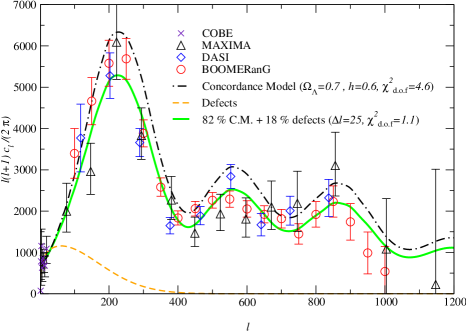
Figure 5: $\ell(\ell+1)C_{\ell}$ versus $\ell$ for three different models. The upper dot-dashed line represents the prediction of a $\Lambda$CDM model. The lower dashed line is a typical string spectrum. Combining both curves with the extra-parameter $\alpha$ produces the solid curve, with a $\chi^{2}$ per degree of freedom slightly above unity. The string contribution turns out to be some $18\%$ of the total bprs .

The quadrupole anisotropy due to freezing in of quantum fluctuations of a scalar field during inflation reads

$$\left(\frac{\delta T}{T}\right)_{\rm Q-infl}=\left[\left(\frac{\delta T}{T}\right)_{\rm Q-scal}^{2}+\left(\frac{\delta T}{T}\right)_{\rm Q-tens}^{2}\right]^{1/2}~{},$$ (38)

with the scalar and tensor contributions given by

$$\left(\frac{\delta T}{T}\right)_{\rm Q-scal}=\frac{1}{4\sqrt{45}\pi}\frac{V^{3/2}(\varphi_{Q})}{M_{\rm Pl}^{3}\,V^{\prime}(\varphi_{Q})}~{},$$ (39)

and

$$\left(\frac{\delta T}{T}\right)_{\rm Q-tens}\sim{0.77\over 8\pi}\,\frac{V^{1/2}(\varphi_{Q})}{M_{\rm Pl}^{2}}~{},$$ (40)

respectively. Here $V$ is the potential of the inflaton field $\varphi$, with $V^{\prime}\equiv{\rm d}V(\varphi)/{\rm d}\varphi$, $M_{\rm Pl}$ denotes the reduced Planck mass, $M_{\rm Pl}={(8\pi G)^{-1/2}}\simeq 2.43\times 10^{18}$ GeV, and $\varphi_{\rm Q}$ is the value of the inflaton field when the comoving scale corresponding to the quadrupole anisotropy became bigger than the Hubble radius.

Simulations of Goto-Nambu local strings in a Friedmann–Lemaître–Roberston–Walker spacetime lead to ls2003

$$\left(\frac{\delta T}{T}\right)_{\rm cs}\sim(9-10)G\mu\quad\mathrm{with}\quad\mu=2\pi\langle\chi\rangle^{2}~{},$$ (41)

where $\langle\chi\rangle$ is the vacuum expectation value of the Higgs field responsible for the formation of cosmic strings.

Before discussing F- and D-term inflation, I would like briefly to describe the curvaton mechanism lw2002 , according which the primordial fluctuations could also be generated from the quantum fluctuations of a late-decaying scalar field, the curvaton field ${\cal\psi}$, which does not play the rôle of the inflaton field. During inflation the curvaton potential is very flat and the curvaton acquires quantum fluctuations, which are expressed in terms of the the expansion rate during inflation, $H_{\rm infl}=\sqrt{(}8\pi G/3)V(\varphi)$, through

$$\delta{\cal\psi}_{\rm init}={H_{\rm inf}\over 2\pi}~{}.$$ (42)

They lead to entropy fluctuations at the end of inflation.

During the radiation-dominated era the curvaton decays and reheats the universe. The primordial fluctuations of the curvaton field are converted to purely adiabatic density fluctuations, thus the curvaton contribution in terms of the metric perturbation reads

$$\left(\frac{\delta T}{T}\right)_{\rm curv}=-{4\over 27}{\delta{\cal\psi_{\rm init}}\over\psi_{\rm init}}~{}.$$ (43)

If one assumes the additional contribution to the temperature anisotropies originated from the curvaton field, then

$$\left[\left(\frac{\delta T}{T}\right)_{\rm tot}\right]^{2}=\left[\left(\frac{\delta T}{T}\right)_{\rm infl}\right]^{2}+\left[\left(\frac{\delta T}{T}\right)_{\rm cs}\right]^{2}+\left[\left(\frac{\delta T}{T}\right)_{\rm curv}\right]^{2}~{}.$$ (44)

The total quadrupole anisotropy, the l.h.s. of Eq. (44), is the one to be normalised to the Cosmic Background Explore (COBE) data cobe , namely $\left(\delta T/T\right)_{\rm Q}^{\rm COBE}\sim 6.3\times 10^{-6}$.

F-term Inflation

Considering only large angular scales one can calculate the contributions to the CMB temperature anisotropies analytically. The quadrupole anisotropy has one contribution coming from the inflaton field, calculated using Eq. (5), and one contribution coming from the cosmic string network. Fixing the number of e-foldings to 60, the inflaton and cosmic string contributions to the CMB depend on the superpotential coupling $\kappa$, or equivalently, on the symmetry breaking scale $M$ associated with the inflaton mass scale, which coincides with the string mass scale.

The total quadrupole anisotropy, to be normalised to the COBE data, is found to be rs1

$$\left({\delta T\over T}\right)_{\rm Q-tot} \sim \Big{\{}y_{\rm Q}^{-4}\left({\kappa^{2}\mathcal{N}\,N_{\rm Q}\over 32\pi^{2}}\right)^{2}\Big{[}\frac{64N_{\rm Q}}{45\cal N}x_{\rm Q}^{-2}y_{\rm Q}^{-2}f^{-2}(x_{Q}^{2})$$ (45)

$$~{}~{}~{}~{}~{}~{}~{}~{}~{}~{}~{}~{}~{}~{}~{}~{}~{}~{}~{}~{}~{}~{}~{}~{}~{}+\left(\frac{0.77\kappa}{\pi}\right)^{2}+324\Big{]}\Big{\}}^{1/2}~{}.$$

In Eq. (45),

$$x_{\rm Q}={|S_{\rm Q}|\over M}~{}~{};~{}~{}y_{\rm Q}^{2}=\int_{1}^{x_{\rm Q}^{2}}\frac{{\rm d}z}{zf(z)}$$ (46)

and

$$N_{\rm Q}=\frac{4\pi^{2}}{\kappa^{2}\cal N}\frac{M^{2}}{M_{\rm Pl}^{2}}\,y_{\rm Q}^{2}~{},$$ (47)

with

$$f(z)=(z+1)\ln(1+z^{-1})+(z-1)\ln(1-z^{-1})~{}.$$ (48)

As noted earlier, the index _Q denotes the scale responsible for the quadrupole anisotropy in the CMB.

The cosmic string contribution is consistent with the CMB measurements provided rs1

$$M\hbox{ \raise 1.50696pt\hbox to0.0pt{$<$\hss}\lower 2.58334pt\hbox{$\sim$}\ }2\times 10^{15}{\rm GeV}~{}~{}\Leftrightarrow~{}~{}\kappa\hbox{ \raise 1.50696pt\hbox to0.0pt{$<$\hss}\lower 2.58334pt\hbox{$\sim$}\ }7\times 10^{-7}~{}.$$ (49)

Strictly speaking the above condition was found in the context of SO(10) gauge group, but the conditions imposed in the case of other gauge groups are of the same order of magnitude since $M$ is a slowly varying function of the dimensionality ${\cal N}$ of the representations to which the scalar components of the chiral Higgs superfields belong rs1 .

The superpotential coupling $\kappa$ is also subject to the gravitino constraint, which imposes an upper limit to the reheating temperature to avoid gravitino overproduction. Within the framework of SUSY GUTs and assuming the see-saw mechanism to give rise to massive neutrinos, the inflaton field decays during reheating into pairs of right-handed neutrinos. This constraint on the reheating temperature can be converted into a constraint on the superpotential coupling $\kappa$. The gravitino constraint on $\kappa$ reads rs1 $\kappa\hbox{ \raise 1.50696pt\hbox to0.0pt{$<$\hss}\lower 2.58334pt\hbox{$\sim$}\ }8\times 10^{-3}$, which is a weaker constraint than the one obtained from the CMB, Eq. (49).

The tuning of the free parameter $\kappa$ can be softened if one allows for the curvaton mechanism. Clearly, within supersymmetric theories such scalar fields are expected to exist. In addition, embedded strings, if they accompany the formation of cosmic strings, they may offer a natural curvaton candidate, provided the decay product of embedded strings gives rise to a scalar field before the onset of inflation. Considering the curvaton scenario, the coupling $\kappa$ is only constrained by the gravitino limit. More precisely, assuming the existence of a curvaton field there is an additional contribution to the temperature anisotropies. Calculating the curvaton contribution to the temperature anisotropies, one obtains the additional contribution rs1

$$\left[\left({\delta T\over T}\right)_{\rm curv}\right]^{2}=y_{Q}^{-4}\,\left({\kappa^{2}\mathcal{N}N_{\rm Q}\over 32\pi^{2}}\right)^{2}\,\left[\left(\frac{16}{81\pi\sqrt{3}}\right)\,\kappa\,\left(\frac{M_{\rm Pl}}{{\cal\psi}_{\rm init}}\right)\right]^{2}~{}.$$ (50)

Normalising the total $\left(\delta T/T\right)_{\rm Q}$ (i.e. the inflaton, cosmic string and curvaton contributions) to the data one gets rs1 the following limit on the initial value of the curvaton field

$${\cal\psi}_{\rm init}\hbox{ \raise 1.50696pt\hbox to0.0pt{$<$\hss}\lower 2.58334pt\hbox{$\sim$}\ }5\times 10^{13}\,\left(\frac{\kappa}{10^{-2}}\right){\rm GeV}~{}~{}\mbox{for}~{}~{}\kappa\in[10^{-6},~{}1].$$ (51)

Finally, I would like to point out that in the case of F-term inflation, the linear mass density $\mu$ (see, Eq. (41)) gets a correction due to deviations from the Bogomol’nyi limit, enlarging the parameter space for F-term inflation enlarge . More precisely, this correction to $\mu$ turns out to be proportional to $\ln(2/\beta)^{-1}$, where $\beta$ is proportional to the square of the ratio between the superpotential and the GUT couplings. Thus, under the assumption that strings contribute less than 10$\%$ to the power spectrum at $\ell=4$, the bound on $\kappa$ reduces to the one imposed by the gravitino limit.

D-term Inflation

D-term inflation leads to cosmic string formation at the end of the inflationary era. The total quadrupole temperature anisotropy, to be normalised to the COBE data, reads rs1

$$\left({\delta T\over T}\right)_{\rm Q}^{\rm tot} \sim \frac{\xi}{M_{\rm Pl}^{2}}\Big{\{}\frac{\pi^{2}}{90g^{2}}x^{-4}_{\rm Q}f^{-2}(x^{2}_{\rm Q})\frac{{\rm W}(x^{2}_{\rm Q}(g^{2}\xi)(\lambda^{2}M_{\rm Pl}^{2}))}{\left[1+{\rm W}(x^{2}_{\rm Q}(g^{2}\xi)(\lambda^{2}M_{\rm Pl}^{2}))\right]^{2}}$$ (52)

$$~{}~{}~{}~{}~{}~{}~{}+\left(\frac{0.77g}{8\sqrt{2}\pi}\right)^{2}+\left(\frac{9}{4}\right)^{2}\Big{\}}^{1/2}~{},$$

where the only unknown is the Fayet-Iliopoulos term $\xi$, for given values of $g$ and $\lambda$. Note that ${\rm W}(x)$ is the “W-Lambert function”, i.e. the inverse of the function $F(x)=xe^{x}$. Thus, one can get $\xi$ numerically, and then obtain $x_{\rm Q}$, as well as the inflaton and cosmic string contribution, as a function of the superpotential and gauge couplings $g$ and $\lambda$. In the case of minimal SUGRA, consistency between CMB measurements and theoretical predictions impose rs1 ; prl2005

$$g\hbox{ \raise 1.50696pt\hbox to0.0pt{$<$\hss}\lower 2.58334pt\hbox{$\sim$}\ }2\times 10^{-2}~{}~{}\mbox{and}~{}~{}\lambda\hbox{ \raise 1.50696pt\hbox to0.0pt{$<$\hss}\lower 2.58334pt\hbox{$\sim$}\ }3\times 10^{-5}~{},$$ (53)

which can be expressed as a single constraint on the Fayet-Iliopoulos term $\xi$,

$$\sqrt{\xi}\hbox{ \raise 1.50696pt\hbox to0.0pt{$<$\hss}\lower 2.58334pt\hbox{$\sim$}\ }2\times 10^{15}~{}{\rm GeV}~{}.$$ (54)

These results are shown in Fig. (6).

Figure 6: At the top, the cosmic string contribution to he CMB, as a function of the mass scale $\sqrt{\xi}$ in units of $10^{15}{\rm GeV}$. At the bottom, cosmic string contribution to the CMB temperature anisotropies, as a function of the superpotential coupling $\lambda$, for different values of the gauge coupling $g$. The maximal contribution allowed by WMAP is represented by a dotted line prl2005 .

The fine tuning on the couplings can be softened if one invokes the curvaton mechanism. Calculating the curvaton contribution to the temperature anisotropies, one obtains the additional contribution prl2005

$$\left[\left({\delta T\over T}\right)_{\rm curv}\right]^{2}=\frac{1}{6}\,\left(\frac{2}{27\pi}\right)^{2}\,\left(\frac{g\xi}{M_{\rm Pl}\psi_{\rm init}}\right)^{2}~{}.$$ (55)

Thus, the gauge coupling can reach the upper bound imposed from the gravitino mechanism, provided the initial value of the curvaton field is prl2005

$$\psi_{\rm init}\hbox{ \raise 1.50696pt\hbox to0.0pt{$<$\hss}\lower 2.58334pt\hbox{$\sim$}\ }3\times 10^{14}\left(\frac{g}{10^{-2}}\right){\rm GeV}~{}~{}\mbox{for}~{}~{}\lambda\in[10^{-1},10^{-4}]~{};$$ (56)

for smaller values of $\lambda$, the curvaton mechanism is not necessary. This result is explicitly shown in Fig. (7).

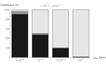
Figure 7: The cosmic string (dark grey), curvaton (light grey) and inflaton (grey) contributions to the CMB temperature anisotropies as a function of the the initial value of the curvaton field ${\cal\psi}_{\rm init}$, for $\lambda=10^{-1}$ and $g=10^{-1}$ prl2005 .

Concluding, within minimal supergravity the couplings and masses must be fine tuned to achieve compatibility between measurements on the CMB temperature anisotropies and theoretical predictions. Note that for minimal D-term inflation, one can neglect the corrections introduced by the superconformal origin of supergravity.

The constraints on the couplings remain qualitatively valid in non-minimal supergravity theories; the superpotential $W$ given in Eq. (7) and we consider a non-minimal Kähler potential. Let us first consider D-term inflation based on Kähler geometry with shift symmetry. If we identify the inflaton field with the real part of $S$ then we obtain the same constraint for the superpotential coupling as in the minimal supergravity case. However, if the inflaton field is the imaginary part of $S$, then we get that the the cosmic string contribution becomes dominant, in contradiction with the CMB measurements, unless the superpotential coupling is rs3

$$\lambda\hbox{ \raise 1.50696pt\hbox to0.0pt{$<$\hss}\lower 2.58334pt\hbox{$\sim$}\ }3\times 10^{-5}~{}.$$ (57)

We show this constraint in Fig. (8).

Figure 8: Cosmic string contribution to the CMB temperature anisotropies as a function of $\lambda$, in the case of D-term inflation based on a Kähler geometry with shift symmetry. The inflaton field is identified with the imaginary part rs3 .

Considering D-term inflation based on a Kähler potential with non-renormalisable terms, the contribution of cosmic strings dominates if the superpotential coupling $\lambda$ is close to unity. Setting $f_{\pm}(|S|^{2}/M_{\rm Pl}^{2})=c_{\pm}(|S|^{2}/M_{\rm Pl}^{2})$, we find that in the simplified case $b=0$ (see, Eq. (18)), the constraints on $\lambda$ read rs3

$$(0.1-5)\times 10^{-8}\leq\lambda\leq(2-5)\times 10^{-5}$$ (58)

or equivalently

$$\sqrt{\xi}\leq 2\times 10^{15}\;\mathrm{GeV}~{},$$ (59)

implying

$$G\mu\leq 8.4\times 10^{-7}~{}.$$ (60)

In the general case, where $b\neq 0$, the constraints are shown in Fig. (9).

Figure 9: Cosmic string contribution to the CMB temperature anisotropies as a function of $\lambda$, in the case of D-term inflation based on a Kähler potential with non-renormalisable terms rs3 . In the top panel we set $g=10^{-2}$ and $c_{\pm}=0$; the simple case $b=0$ is represented by the dashed line, while plain lines show the contributions for $b=0.5,1,2$, going from the bottom to the top rs3 . In the bottom panel we set $b=1$ and $c_{\pm}=1$; the plain lines show the contributions for $g=10^{-3},10^{-2},10^{-1}$, going from bottom to the top rs3 .

In conclusion, higher order Kähler potentials do not suppress cosmic string contribution, as it was incorrectly claimed in the literature. By allowing a small, but non-negligible, contribution of strings to the angular power spectrum of CMB anisotropies, we constrain the couplings of the inflationary models, or equivalently the dimensionless string tension. These models remain compatible with the most current CMB measurements, even when one calculates ns the spectral index. More precisely, the inclusion of a sub-dominant string contribution to the large scale power spectrum amplitude of the CMB, increases the preferred value for the spectral index ns .

Brane Inflation

The CMB temperature anisotropies originate from the amplification of quantum fluctuations during inflation, as well as from the cosmic superstring network. If the scaling regime of the superstring network is the unique source of the density perturbations, the COBE data yield $G\mu\simeq 10^{-6}$. Using the latest WMAP data, the contribution from strings to the total CMB power spectrum on observed scales is at most 10$\%$, which translates in the upper limit on the dimensionless string tension $G\mu\hbox{ \raise 1.50696pt\hbox to0.0pt{$<$\hss}\lower 2.58334pt\hbox{$\sim$}\ }1.8\ (2.7)\times 10^{-7}$ at $68\ (95)\%$ confidence pog . Thus, the cosmic superstrings produced towards the end of inflation in the context of braneworld cosmological models is in agreement with the present CMB data.

5.2 Gravitational Wave Background

Oscillating cosmic string loops emit vil Gravitational Waves (GW). Long strings are not straight but they have a superimposed wiggly small-scale structure due to string intercommutations, thus they also emit ms-gw GW. Cosmic superstrings can also generate dv a stochastic GW background. Therefore, provided the emission of gravity waves is the efficient mechanism cmf ; gwandstrings for the decay of string loops, cosmic strings/superstrings could provide a source for the stochastic GW spectrum in the low-frequency band. The stochastic GW spectrum has an almost flat region in the frequency range $10^{-8}-10^{10}$ Hz. Within this window, both ADVANCED LIGO/VIRGO (sensitive at a frequency $f\sim 10^{2}$ Hz) and LISA (sensitive at $f\sim 10^{-2}$ Hz) interferometers may have a chance of detectability.

Strongly focused beams of relatively high-frequency GW are emitted by cusps and kinks in oscillating strings/superstrings. The distinctive waveform of the emitted bursts of GW may be the most sensitive test of strings/superstrings. ADVANCED LIGO/VIRGO may detect bursts of GW for values of $G\mu$ as low as $10^{-13}$, and LISA for values down to $G\mu\geq 10^{-15}$. At this point, I would like to remind to the reader that there is still a number of theoretical uncertainties for the evolution of a string/superstring network gwandstrings .

Recently, they have been imposed limits pulsar on an isotropic gravitational wave background using pulsar timing observations, which offer a chance of studying low-frequency (in the range between $10^{-9}-10^{-7}$ Hz) gravitational waves. The imposed limit on the energy density of the background per unit logarithmic frequency interval reads $\Omega_{\rm GW}^{\rm cs}(1/8{\rm yr})h^{2}\leq 1.9\times 10^{-8}$ (where $h$ stands for the dimensionless amplitude in GW bursts).

If the source of the isotropic GW background is a cosmic string/superstring network, then it leads to an upper bound on the dimensionless tension of a cosmic string/superstring background. Under reasonable assumptions for the string network the upper bound on the string tension reads pulsar $G\mu\leq 1.5\times 10^{-8}$. This is a strongest limit than the one imposed from the CMB temperature anisotropies. Thus, F- and D-term inflation become even more fine tuned, unless one invokes the curvaton mechanism.

This limit does not affect cosmic superstrings. However, it has been argued pulsar that with the full Parkes Pulsar Timing Array (PPTA) project the upper bound will become $G\mu\leq 5\times 10^{-12}$, which is directly relevant for cosmic superstrings. In conclusion, the full PPTA will either detect gravity waves from strings and string-like objects, or they will rule out a number of models.

6 Conclusions

Cosmic strings are generically formed at the end of hybrid inflation in a large number of models within supersymmetry and supergarvity theories. String-like objects, which could play the rôle of cosmic strings, are also generically produced at the end of brane inflation, in many brane inflation models in the context of theories with large extra dimensions. These one-dimensional objects would contribute in the generation of fluctuations leading to the observed structure formation and the measured CMB temperature anisotropies. They would also source a stochastic gravity wave background.

Current measurements of the CMB spectrum, as well as of the gravitational wave background, impose severe constraints on the free parameters of the models. More precisely, the dimensionless parameter $G\mu$ must be small enough to avoid contradiction with the currently available data.

The rôle of strings can be suppressed by adding new terms in the superpotential mcdonald , or by considering the curvaton mechanism prl2005 ; endoetal . One can escape the string problem by complicating the models so that the produced strings (D-term strings formed at the end of D-term inflation, or D-strings formed at the end of brane collisions) become unstable (semilocal strings), along the lines of Refs. toine1 ; semilocal . To be more specific, it has been proposed semilocal that introducing additional matter multiplets one obtains a nontrivial global symmetry such as SU(2), leading to a simply connected vacuum manifold and the production of semilocal strings. Later on, it has been suggested toine1 that if the waterfall Higgs fields are non-trivially charged under some other gauge symmetries $H$, such that the vacuum manifold, $[H\times U(1)]/U(1)$, is simply connected, then the strings are semilocal objects.

If the daily improved data require even more severe fine tuning of the models, then I believe that one should develop and subsequently study models where the strings and string-like objects, formed at the end or after inflation, are indeed unstable.

References

- (1) A. H. Guth, Phys. Rev. D 23, 347 (1981); A. D. Linde, Rep. Prog. Phys. 47, 925 (1984).
- (2) T. Piran, Phys. Let. B 181, 238 1986; D. S. Goldwirth, Phys. Rev. D 43, 3204 1991; E. Calzetta and M. Sakellariadou, Phys. Rev. D 45, 2802 1992; E. Calzetta and M. Sakellariadou, Phys. Rev. D 47, 3184 1993.
- (3) G. W. Gibbons and N. Turok, The measure problem in cosmology, [hep-th/0609095]; C. Germani, W. Nelson and M. Sakellariadou, On the onset of inflation in loop quantum cosmology, [gr-qc/0701172].
- (4) A. D. Linde, Phys. Lett. B 129, 177 (1983).
- (5) A. D. Linde, Phys. Lett. B 259, 38 (1991).
- (6) L. A. Kofman and A. D. Linde, Nucl. Phys. B 282, 555 (1987); A. D. Linde and A. Riotto, Phys. Rev. D 56, 1841 (1997); D. H. Lyth and A. Riotto, Phys. Rep. 314, 1 (1999).
- (7) R. Jeannerot, J. Rocher and M. Sakellariadou, Phys. Rev. D 68, 103514 (2003).
- (8) E. Halyo, Phys. Lett. B 387, 43 (1996); P. Binetruy and D. Dvali, Phys. Lett. B 388, 241 (1996).
- (9) C. Coleman, and E. Weinberg, Phys. Rev. D 7, 1888 (1973).
- (10) J. Rocher and M. Sakellariadou, J. Cosm. & Astrop. Phys. 0503, 004 2005.
- (11) P. Binetruy, G. Dvali, R. Kallosh and A. Van Proeyen, Class. & Quant. Grav. 21, 3137 2004.
- (12) J. Rocher, M. Sakellariadou, Phys. Rev. Lett. 94, 011303 2005.
- (13) J. P. Hsu and R. Kallosh, J. High En. Phys. 0404, 042 2004.
- (14) J. Rocher and M. Sakellariadou, J. Cosm. & Astrop. Phys. 0611, 001 2006.
- (15) A. Vilenkin and E. P. S. Shellard; Cosmic Strings and Other Topological Defects (Cambridge University Press, Cambridge, England, 2000); M. B. Hindmarsh and T. W. B. Kibble, Rep. Prog. Phys. 58, 477 (1995).
- (16) T. W. B. Kibble, J. Phys. A 9, 387 (1976).
- (17) N. Turok, Phys. Rev. Lett. 63, 2625 (1989).
- (18) T. Vachaspati and M. Barriola, Phys. Rev. Lett. 69, 1867 (1992).
- (19) M. Sakellariadou: Cosmic Strings. In: Quantum Simulations via Analogues: From Phase Transitions to Black Holes (Springer Lecture Notes in Physics) (to appear), [arxiv:hep-th/0602276].
- (20) T. W. B. Kibble, Nucl. Phys. B 252, 277 (1985).
- (21) A. Albrecht and N. Turok, Phys. Rev. Lett. 54, 1868 (1985); A. Albrecht and N. Turok, Phys. Rev. D 40, 973 (989).
- (22) M. Sakellariadou and A. Vilenkin, Phys. Rev. D 42, 349 (1990); D. P. Bennett, in Formation and Evolution of Cosmic Strings, edited by G. Gibbons, S. Hawking and T. Vachaspati (Cambridge University Press, Cambridge, England, 1990); F. R. Bouchet, ibid; E. P. S. Shellard and B. Allen, ibid.
- (23) C. Ringeval, M. Sakellariadou and F. R. Bouchet, J. Cosm. & Astrop. Phys. 02, 023 2007.
- (24) V. Vanchurin, K. D. Olum and A. Vilenkin, Phys. Rev. D 74, 063527 92006); C. J. A. P. Martins and E. P. S. Shellard, Phys. Rev. D 73, 043515 (2006); K. D. Olum and V. Vanchurin, Cosmic string loops in the expanding universe, [arXiv:astro-ph/0610419].
- (25) Y. Fukuda, et. al., [Super-Kamiokande Collaboration], Phys. Rev. Lett. 81, 1562 (1998); Q. R. Ahmad, et al. [SNO Collaboration], Phys. Rev. Lett. 87, 071301 (2001); K. Eguchi, et al. [KamLAND Collaboration], Phys. Rev. Lett. 90, 021802 (2003).
- (26) P. Horava and E. Witten, Nucl. Phys. B 460, 506 (1996).
- (27) R. Jeannerot and A.-C. Davis, Phys. Rev. D 52, 7220 (1995).
- (28) M. Sakellariadou, Annalen Phys. 15, 264 (2006).
- (29) R. Durrer, M. Kunz and M. Sakellariadou, Phys. Lett. B 614, 12 2005.
- (30) S.-H. Tye, Brane inflation: string theory viewed from the cosmos, [hep-th/0610221].
- (31) E. Witten, Nucl. Phys. B 249, 557 (1985).
- (32) J. Polchinski, Introduction to cosmic F- and D-strings, [hep-th/0412244].
- (33) M. G. Jackson, N. T. Jones and J. Polchinski, J. High En. Phys. 0510, 013 (2005).
- (34) A. Hanany and K. Hashimoto K, JHEP 0506, 021 (2005).
- (35) M. Sakellariadou, J. Cosm. & Astrop. Phys. 0504, 003 (2005); E. Copeland and P. Saffin, J. High En. Phys. 0511, 023 (2005); S.-H. H. Tye, I. Wasserman and M. Wyman, Phys. Rev. D 71, 103508 (2005); Erratum-ibid. Phys. Rev. D 71, 129906 (2005); M. Hindmarsh and P. M. Saffin, J. High En. Phys. 0608, 066 (2006).
- (36) J. Martin, A. Riazuelo, and M. Sakellariadou, Phys. Rev. D 61, 083518 (2002); A. Gangui, J. Martin, and M. Sakellariadou, Phys. Rev. D 66, 083502 (2002).
- (37) S. Veeraraghavan and A. Stebbins, Ap. J. 365, 37 (1990).
- (38) G. Vincent, M. B. Hindmarsh and M. Sakellariadou, Phys. Rev. D 55, 573 (1997).
- (39) U.-L. Pen, U. Seljak and N. Turok Phys. Rev. Lett. 79, 1611 (1997).
- (40) R. Durrer, A. Gangui and M. Sakellariadou, Phys. Rev. Lett. 76, 579 (1996).
- (41) R. Durrer, M. Kunz, C. Lineweaver and M. Sakellariadou, Phys. Rev. Lett. 79, 5198 (1997); R. Durrer, M. Kunz and A. Melchiorri, Phys. Rev. D 59, 123005 (1999).
- (42) U.-L. Pen, U. Seljak and N. Turok, Phys. Rev. Lett. 79, 1611 (1997); N. Turok, U.-L. Pen and U. Seljak, Phys. Rev. D 58, 023506 (1998).
- (43) R. Durrer and M. Sakellariadou, Phys. Rev. D 56, 4480 (1997).
- (44) N. Bevis, M. Hindmarsk, M. Kunz and J. Urrestilla, CMB power spectrum contribution from cosmic strings using field-evolution simulations of the Abelian Higgs model, [arXiv:astro-ph/0605018].
- (45) D. N. Spergel, et. al., Wilkinson Microwave Anisotropy Probe (WMAP) Three Year Results: Implications for Cosmology, [arXiv:astro-ph/0603449].
- (46) F. R. Bouchet, P. Peter,A. Riazuelo and M. Sakellariadou, Phys. Rev. D 65, 021301(R) (2001).
- (47) M. Landriau, and E. P. S. Shellard, Phys. Rev. D 69, 023003 (2004).
- (48) D. H. Lyth and D. Wands, Phys. Lett. B 524, 5 (2002); T. Moroi, and T. Takahashi, Phys. Lett. B 522, 215 (2001), Erratum-ibid. B 539, 303 (2002); K. Enqvist, S. Kasuya, and A. Mazumdar, Phys. Rev. Lett. 90, 091302 (2003); K. Dimopoulos and D. Lyth, Phys. Rev. D 69, 123509 (2004).
- (49) C. L. Bennett, et. al. Astrophys. J. 464, 1 (1996).
- (50) R. Jeannerot and M. Postma, J. Cosm. & Astrop. Phys. 0607, 012 2006.
- (51) R. A. Battye, B. Garbrecht and A. Moss, J. Cosm. & Astrop. Phys. 0609, 007 2006.
- (52) M. Wyman, L. Pogosian and I. Wasserman, Phys. Rev. D 72, 023513 (2005); Erratum-ibid. D73, 089904 (2006).
- (53) A. Vilenkin, Phys. Lett. B 107, 47 (1981).
- (54) M. Sakellariadou, Phys. Rev. D 42, 354 (1990).
- (55) T. Damour and A. Vilenkin, Phys. Rev. D 71, 063510 (2005); X. Siemens, et. al. Phys. Rev. D 73, 105001 (2006); X. Siemens, V. Mandic and J. Creighton, Gravitational wave stochastic background from cosmic (super)strings, [astro-ph/0610920 ].
- (56) G. R. Vincent, M. Hindmarsh and M. Sakellariadou, Phys. Rev. D 56, 637 (1997); G. R. Vincent, N. D. Antunes and M. Hindmarsh, Phys. Rev. Lett. 80, 2277 (1998).
- (57) F. A. Jenet, et al., Upper bounds on the low-frequency stochastic gravitational wave background from pulsar timing observations: current limits and future prospects, [astro-ph/0609013].
- (58) C.-M. Lin and J. McDonald, Phys. Rev. D 74, 063510 (2006).
- (59) M. Endo, M. Kawasaki abd T. Moroi, Phys. Lett. B 569, 73 (2003).
- (60) J. Urrestilla, A. Achúcarro and A. C. Davis, Phys. Rev. Lett. 92, 251302 (2004).