Gauss-Bonnet cosmologies: crossing the phantom divide and the transition from matter dominance to dark energy

Abstract:

Dark energy cosmologies with an equation of state parameter $w$ less than $-1$ are often found to violate the null energy condition and show unstable behaviour. A solution to this problem may require the existence of a consistent effective theory that violates the null energy condition only momentarily and does not develop any instabilities or other pathological features for a late time cosmology. A model which incorporates a dynamical scalar field $\varphi$ coupled to the quadratic Riemann invariant of the Gauss-Bonnet form is a viable proposal. Such an effective theory is shown to admit nonsingular cosmological evolutions for a wide range of scalar-Gauss-Bonnet coupling. We discuss the conditions for which our model yields observationally supported spectra of scalar and tensor fluctuations, under cosmological perturbations. The model can provide a reasonable explanation for the transition from matter dominance to dark energy regime and the late time cosmic acceleration, offering an interesting testing ground for investigations of the cosmological modified gravity.

1 Introduction and Overview

Dark energy and its associated cosmic acceleration problem has been presented as three well posed conundrums in modern cosmology: (1) why the dark energy equation of state $w_{\lower 2.0pt\hbox{$\scriptstyle\rm DE$}}$ is so close to $-1$, (2) why the dark energy density is comparable to the matter density now, the so-called cosmic coincidence problem, and (3) why the cosmological vacuum energy is small and positive. Additionally, we do not yet have a good theoretical understanding of the result that the expansion of our universe is accelerating after a long period of deceleration as inferred from the observations of type Ia supernovae, gravitational weak lensing and cosmic microwave background (CMB) anisotropies  [1, 2]; for review, see, e.g. [3].

A possible source of the late time acceleration is given by vacuum energy with a constant equation of state, known as the cosmological constant, or a variant of it, quintessence [4]. Several plausible cosmological scenarios have also been put forward to explain these problems within the context of modified theories of scalar-tensor gravity such as, coupled quintessence [5], k-inflation or dilatonic-ghost model [6], scalar-phantom model [7], Gauss-Bonnet dark energy [8] and its various generalizations [9, 10, 11]. These ideas are interesting as, like quintessence, they offer a possible solution to the cosmic coincidence problem. The proposals in [7, 8, 9, 10, 11] are promising because they may lead to the observationally supported equation of state, $w\approx-1$, while more interestingly provide a natural link between cosmic acceleration and fundamental particle theories, such as superstring theory. In this paper we will focus primarily on the first two questions raised above within the context of a generalized theory of scalar-tensor gravity that includes the Gauss-Bonnet curvature invariant coupled to a scalar field $\varphi$.

The question of whether the gravitational vacuum energy is something other than a pure cosmological term will not be central to our discussion. But we note that Einstein’s general relativity supplemented with a cosmological constant term does not appear to have any advantages over scalar-tensor gravity containing a standard scalar potential. The recent observation that the dark energy equation of state parameter $w$ is $\approx-1$ does not necessarily imply that the dark energy is in the form of a cosmological constant; it is quite plausible that after inflation the scalar field $\varphi$ has almost frozen, so that $V(\phi)\approx{\rm const}=\Lambda$. In a cosmological background, there is no deep reason for expecting the energy density of the gravitational vacuum to be a constant, instead perhaps it can be determined by the underlying theory, as in the case where a scalar potential possesses many minima. It is thus worth exploring dynamical dark energy models, supporting both $w<-1$ and $w>-1$, and also $w^{*}(z)\equiv dw/dz\neq 0$ (where $z$ is the redshift parameter).

The expansion of the universe is perhaps best described by a monotonically decreasing Hubble expansion rate, implying that $\dot{H}\equiv\ddot{a}/a-\dot{a}^{2}/a^{2}\leq 0$, where $a=a(t)$ is the scale factor of a four-dimensional Friedmann-Robertson-Walker universe and the dot represents a derivative with respect to the cosmic time $t$. In the presence of a barotropic fluid of pressure $p$ and energy density $\rho$, this last inequality implies that the cosmic expansion obeys the null energy condition (NEC), $p+\rho\geq 0$, and hence $w\equiv p/\rho\geq-1$. The standard view is that the Hubble expansion rate increases as we consider earlier epochs until it is of a similar order to that of the Planck mass, $m_{Pl}\sim{10}^{18}\,GeV$. However, in strong gravitational fields, such as, during inflation, the Einstein description of gravity is thought to break down and quantum gravity effects are expected to become important. This provides a basis for the assumption that the expansion of the universe is inseparable from the issue of the ultraviolet completion of gravity. In recent years, several proposals have been made in order to establish such a link. For instance, reference [12] introduced a system of a derivatively coupled scalar Lagrangian which violates the condition $\dot{H}\leq 0$ spontaneously: the model would involve a short-scale (quantum) instability associated with a super-luminal cosmic expansion (see also [13]).

The beauty of Einstein’s theory is in its simplicity. It has been remarkably successful as a classical theory of gravitational interactions from scales of millimeters through to kiloparsecs. Thus any modification of Einstein’s theory, both at small and large distance scales, must be consistent with known tests. Several proposals in the literature, e.g. in [12, 14], do not seem to fall into this category as these ideas would involve modifications of Einstein’s theory in a rather non-standard (and non-trivial) way.

We motivate our work through the theoretical insights of superstring or M-theory as it would appear worthwhile to explore the cosmological implications of such models. In this paper we examine whether we can achieve observationally supported cosmological perturbations in the low-energy string effective action, which includes a non-trivial interaction between a dynamical scalar field $\varphi$ and a Riemann invariant of the Gauss-Bonnet form, and study its phenomenological viability as a dark energy model. It is appreciated that a generalized theory of scalar-tensor gravity, featuring one or several scalar fields coupled to a spacetime curvature, or a Riemann curvature invariant, can easily account for an accelerated universe with quintessence ($w>-1$), cosmological constant ($w=-1$) or phantom ($w<-1$) equation of state without introducing the wrong sign on the scalar kinetic term.

This paper is organised as follows. In the following section we discuss a general scalar-field Lagrangian framework and write equations of motion that describe gravity and a scalar field $\varphi$, allowing non-trivial matter-scalar couplings. We discuss some astrophysical and cosmological constraints on the model. In section 3 we present the construction of a number of scalar potentials for some specific constraints, in an attempt to gain insight into the behaviour of the scalar potential for late time cosmology. In section 4 we discuss inflationary cosmologies for specific cases and study the parameters related to cosmological perturbations of the background solution. The problem of suitable initial conditions, given stable observationally viable solutions with a full array of background fields for the general system is considered in section 5 using numerical and analytic techniques for both minimal and non-minimal scalar-matter couplings. In section 6 we present several remarks about the existence of superluminal propagation and/or short-scale negative instabilities for the tensor modes. Section 7 is devoted to the discussions of our main results.

2 Essential Ingredients

An unambiguous and natural way of modifying Einstein’s General Relativity in four dimensions is to introduce one or more fundamental scalar fields and their interactions with the leading order curvature terms in the $\alpha^{\prime}$ expansion, as arising in string or M theory compactifications from ten- or eleven-dimensions to four-dimensions. The simplest version of such scalar-tensor gravities, which is sufficiently general for explaining the cosmological evolution of our universe, may be given by

$$S=S_{grav}+S_{m},$$ (1)

with the following general action

$$S_{grav} = \int d^{4}{x}\sqrt{-g}\left(\frac{R}{2\kappa^{2}}-\frac{\gamma}{2}\,(\nabla\varphi)^{2}-V(\varphi)-\frac{1}{8}f(\varphi){\cal R}_{GB}^{2}\right),$$ (2)

$$S_{m} = S(\varphi,A^{2}(\varphi)g_{\mu\nu},\psi_{m})=\int d^{4}x\sqrt{-g}\left(A^{4}(\varphi)\left(\rho_{m}+\rho_{r}\right)\right),$$ (3)

where ${{\cal R}_{GB}^{2}}\equiv R^{2}-4\,R_{\mu\nu}\,R^{\mu\nu}+R_{\mu\nu\rho\sigma}\,R^{\mu\nu\rho\sigma}$ is the Gauss-Bonnet (GB) curvature invariant. We shall assume that $\varphi$ is a canonical field, so $\gamma>0$. The coupling $f(\varphi)$ between $\varphi$ and the GB term is a universal feature of all four-dimensional manifestations of heterotic superstring and M theory [15, 16]. For example, such a form arises at heterotic string tree-level if $\varphi$ represents a dilaton, and at one-loop level if $\varphi$ represents the average volume modulus; in a known example of heterotic string theory, one has $f(\varphi)\propto\sum_{n=1}c_{n}\,e^{(n-2)\varphi}>0$ in the former case, while $f(\varphi)\propto\varphi-\frac{\pi}{3}\,e^{\varphi}+4\sum_{n=1}\ln\left(1-e^{-2n\pi\,e^{\varphi}}\right)+\ln 2<0$ in the latter case (see also discussions in  [17]). As discussed in [10, 11], a non-trivial or non-constant $f(\varphi)$ is useful not only for modelling a late time cosmology but also desirable for embedding the model in a fundamental theory, such as superstring theory. Here we also note that from a model building point of view, only two of the functions $V(\varphi),f(\varphi)$ and $A(\varphi)$ are independent; these can be related through the Klein-Gordan equation (see below).

One can supplement the above action with other higher derivative terms, such as those proportional to $f(\varphi)(\nabla_{\lambda}\varphi\nabla^{\lambda}\varphi)^{2}$ and curvature terms, but in such cases it would only be possible to get approximate (asymptotic) solutions, so we limit ourselves to the above action. In the model previously studied by Antoniadis et al. [15], $V(\varphi)$ and $S_{m}$ were set to zero. However, the states of string or M theory are known to include extended objects of various dimensionalities, known as ‘branes, beside trapped fluxes and non-trivial cycles or geometries in the internal (Calabi-Yau) spaces. It is also natural to expect a non-vanishing potential to arise in the four-dimensional string theory action due to some non-pertubative effects of branes and fluxes. With supersymmetry broken, such a potential can have isolated minima with massive scalars, this then avoids the problem with runway behaviour of $\varphi$ after inflation.

In this paper we fully extend the earlier analysis of the model in [10] by introducing background matter and radiation fields. We allow $\varphi$ to couple with both an ordinary dust-like matter and a relativistic fluid. We show that the model under consideration is sufficient to solve all major cosmological conundrums of concordance cosmology, notably the transition from matter dominance to a dark energy regime and the late time cosmic acceleration problem attributed to dark energy, satisfying $w_{\rm eff}\approx-1$.

2.1 Basic equations

In order to analyse the model we take a four-dimensional spacetime metric in standard Friedmann-Robertson-Walker (FRW) form: $ds^{2}=-dt^{2}+a^{2}(t)\sum_{i=1}^{3}(dx^{i})^{2}$, where $a(t)$ is the scale factor of the universe. The equations of motion that describe gravity, the scalar field $\varphi$, and the background fluid (matter and radiation) are given by

$$-\frac{3}{\kappa^{2}}+3\dot{\varphi}Hf_{,\,\varphi}+\frac{\gamma}{2}x^{2}+{y}+3\Omega_{b} = 0,$$ (4)

$$\frac{1}{\kappa^{2}}\left(2\epsilon+3\right)+\frac{\gamma}{2}x^{2}-y-\ddot{f}-2\dot{\varphi}Hf_{,\,\varphi}(1+\epsilon)+3w_{b}\Omega_{b} = 0,$$ (5)

$$\gamma\left(\ddot{\varphi}+3H\,\dot{\varphi}\right)+V_{,\,\varphi}+{3}\left(1+\epsilon\right)f_{,\,\varphi}H^{4}-\eta QA^{4}\rho_{m} = 0,$$ (6)

where $\ddot{f}\equiv f_{,\,\varphi\varphi}\,\dot{\varphi}^{2}+f_{,\,\varphi}\,\ddot{\varphi}$, $V_{,\,\varphi}\equiv dV/d\varphi$, $\eta$ is a numerical parameter which we define below and

$$\epsilon=\frac{\dot{H}}{H^{2}},\quad{x}=\frac{\dot{\varphi}}{H},\quad y=\frac{V(\varphi)}{H^{2}},\quad w_{b}\equiv\frac{p_{b}}{\rho_{b}},\quad\Omega_{b}\equiv\frac{\rho_{b}A^{4}}{3H^{2}},\quad Q\equiv\frac{d\ln A(\varphi)}{d\varphi},$$ (7)

where $b$ stands for the background matter and radiation. Let us also define

$$\Omega_{\varphi}\equiv\frac{\rho_{\varphi}}{3H^{2}}=\frac{\gamma x^{2}+2y}{6},\qquad u\equiv f_{,\,\varphi}H^{2},\qquad\Omega_{GB}=\dot{\varphi}Hf_{,\,\varphi}=ux\equiv\mu,$$ (8)

so that the constraint equation (4) reads $\Omega_{\varphi}+\Omega_{GB}+\Omega_{b}=1$. The density fraction $\Omega_{b}$ may be split into radiation and matter components: $\Omega_{b}=\Omega_{r}+\Omega_{m}$ and $w_{b}\Omega_{b}=w_{m}\Omega_{m}+w_{r}\Omega_{r}$. Similarly, in the component form, $Q\rho_{m}=Q_{i}\rho_{m}^{(i)}$. Stiff matter for which $w_{m}=1$ may also be included. The analysis of Steinhardt and Turok [18] neglects such a contribution, where only the ordinary pressureless dust ($w_{m}=0$) and radiation ($w_{r}=1/3$) were considered, in a model with $f(\varphi)=0$. The implicit assumption above is that matter couples to $A^{2}(\varphi)g_{\mu\nu}$ with scale factor $\hat{a}$, where $\hat{a}\equiv aA(\varphi)$, rather than the Einstein metric $g_{\mu\nu}$ alone, and $\rho_{r}\propto 1/\hat{a}^{4}$, so $\rho_{r}$ does not enter the $\varphi$ equation of motion, (6). That is, by construction, the coupling of $\varphi$ to radiation is vanishing. This is, in fact, consistent with the fact that the quantity $Q$ couples to the trace of the matter stress tensor, $g_{(i)}^{\mu\nu}T_{\mu\nu}^{(i)}$, which is vanishing for the radiation component, $T_{\mu}^{\mu}=-\rho_{\lower 2.0pt\hbox{$\scriptstyle r$}}+3P_{\lower 2.0pt\hbox{$\scriptstyle r$}}=0$. We also note that, in general, $\rho\propto 1/\hat{a}^{3(1+w)}$, thus, for ordinary matter or dust ($w=0$), we have $\eta=1$, while for a highly relativistic matter ($w=1$), we have $\eta=-2$. Especially, for radiation ($w=1/3$), we have $\eta=0$; while, for any other relativistic matter having a pressure $\rho>p>\rho/3$, $-2<\eta<0$.

Equations (4)-(6) may be supplemented with the equation of motion for a barotropic perfect fluid, which is given by

$$\hat{a}\frac{d\rho_{b}}{d\hat{a}}=\frac{1}{H}\frac{\partial\rho_{b}}{\partial t}+\frac{\dot{\varphi}}{H}\frac{\partial\rho_{b}}{\partial\varphi}=-3(1+w_{b})\rho_{b},$$ (9)

where $p_{b}$ is the pressure of the fluid component with energy density $\rho_{b}$. In the case of minimal scalar-matter coupling, the quantity $\partial\rho_{b}/\partial\varphi\to 0$  and hence

$$\Omega_{b}^{\prime}+2\epsilon\Omega_{b}+3(1+w_{b})\Omega_{b}=0,$$ (10)

where the prime denotes a derivative with respect to $\Delta N=\ln[a(t)]+{\rm const}$ and $a(t)$ is the scale factor of a four-dimensional Friedman-Robertson-Walker universe. In this case the dynamics in a homogeneous and isotropic FRW spacetime may be determined by specifying the field potential $V(\varphi)$ and/or the scalar-GB coupling $f(\varphi)$.

For $A(\varphi)\neq{\rm const}$, there exists a new parameter, $Q$; more precisely,

$$\frac{\partial\rho_{m}^{(i)}}{\partial\varphi}=-\eta\rho_{m}^{(i)}Q_{i},\quad\frac{\partial\rho_{r}}{\partial\varphi}=0.$$ (11)

The variation in the energy densities of the ordinary matter, $\rho_{m}^{(d)}$, and the relativistic fluid, $\rho_{m}^{(s)}$, and their scalar couplings $Q_{i}$ are not essentially the same. Thus, hereafter, we denote the $Q$ by $Q_{d}$ for an ordinary matter (or dust) and $Q_{s}$ for a relativistic matter (or stiff fluid coupled to $\varphi$). Equation (9) may be written as

$$\Omega_{\lower 2.0pt\hbox{$\scriptstyle m,s$}}^{\prime}+2\epsilon\Omega_{\lower 2.0pt\hbox{$\scriptstyle m,s$}}+3(1+w_{m})\Omega_{m,s} = -3\eta Q_{\lower 2.0pt\hbox{$\scriptstyle s$}}\Omega_{m,s}\varphi^{\prime},$$ (12)

$$\Omega_{m,d}^{\prime}+2\epsilon\Omega_{m,d}+3\Omega_{m,d} = -3Q_{\lower 2.0pt\hbox{$\scriptstyle d$}}\Omega_{\lower 2.0pt\hbox{$\scriptstyle m,d$}}\varphi^{\prime},$$ (13)

$$\Omega_{r}^{\prime}+2\epsilon\Omega_{r}+4\Omega_{r} = 0.$$ (14)

For a slowly rolling scalar (or dark energy) field $\varphi$, satisfying $\Delta\varphi\propto\Delta N$ (where $N\equiv\ln[a(t)]$ is the e-folding time), $Q_{d}$ is dynamically determined, for any $f(\varphi)$, by the relation

$$\Omega_{\lower 2.0pt\hbox{$\scriptstyle r$}}=Q_{d}\varphi^{\prime}{\Omega_{\lower 2.0pt\hbox{$\scriptstyle m,d$}}}.$$ (15)

For $\Omega_{r}\sim\Omega_{\lower 2.0pt\hbox{$\scriptstyle m,d$}}$, the scalar field presumably couples strongly to matter. However, for the present value of $\Omega_{\lower 2.0pt\hbox{$\scriptstyle r$}}\sim 10^{-4}$ (on large cosmological scales), one would hardly find a noticeable difference between the cases of non-minimal and minimal coupling of $\varphi$ with matter.

In the following we adopt the convention $\kappa^{2}=8\pi G=1$, unless shown explicitly.

2.2 Cosmological and astrophysical constraints

It is generally valid that scalar-tensor gravity models of the type considered in this paper are constrained by various cosmological and astrophysical observations, including the big bang nucleosynthesis bound on the $\varphi$-component of the total energy density and the local gravity experiments. However, the constraints obtained in a standard cosmological setup (for instance, by analyzing the CMB data), which assumes general relativity, that is, $Q=0$, cannot be straightforwardly applied to the present model. The distance of the last scattering surface can be (slightly) modified if the universe at the stage of BBN contained an appreciable amount in energy in $\varphi$-component, like $\Omega_{\varphi}\lesssim 1/6$ (see, e.g. [21]).

The couplings $Q_{d}$ and $Q_{s}$ can be constrained by taking into account cosmological and solar system experiments. We should also note that observations are made of objects that can be classified as visible matter or dust [22, 23]; hence a value of $Q_{d}^{2}\ll 1$ is suggestive to agree with the current observational limits on deviations from the equivalence principle. If we also require $Q_{s}^{2}\ll 1$, then the non-minimal coupling of $\varphi$ with a relativistic fluid may be completely neglected at present, since $\Omega_{s}\ll\Omega_{d}$. In this subsection, as we are more interested on astrophysical and cosmological constraints of the model, we take $\Omega_{s}=0$, without loss of generality.

Under PPN approximations [24], the local gravity constraints on $Q_{d}$ and its derivative loosely imply that

$$m_{Pl}^{2}Q_{d}^{2}\lesssim 10^{-5},\qquad m_{Pl}\,|dQ_{d}/d\varphi|\lesssim{\cal O}(1).$$ (16)

If $A(\varphi)$ is sufficiently flat near the current value of $\varphi=\varphi_{0}$, then these couplings have modest effects on large cosmological scales. Especially, in the case that $A(\varphi)\propto e^{\zeta\kappa\varphi}$, the above constraints may be satisfied only for a small $\zeta$ ($\ll 1$) since $Q_{d}=\zeta$ is constant. On the other hand, if $A(\varphi)\propto\cosh[\zeta\kappa\varphi]$, then $Q_{d}$ is only approximately constant, at late times. Another possibility is that $Q_{d}\propto e^{-\,\zeta\kappa\varphi}$; in this case, however, for the consistency of the model, one also requires a steep potential. In the particular case of $A(\varphi)\propto e^{\zeta\kappa\varphi}$ with $\zeta\sim{\cal O}(1)$ (as one may expect from string theory or particle physics beyond the standard model), it may be difficult to satisfy the local gravity constraints (under PPN approximation), unless there is a mechanism like the one discussed in [25] (see also [26]).

Only in the case $Q_{d}\varphi^{\prime}\gtrsim 1$, is the last term in (13) possibly relevant, leading to a measurable effect including a ‘fifth force causing violations of the equivalence principle (see, e.g., [22]). However, in our model, it is important to realize that the coupling $Q_{d}$ is dynamically determined by the ratio $\Omega_{r}/(\varphi^{\prime}\Omega_{m})$. Even if we allow a small slope for the time variation of the field, $\varphi^{\prime}\simeq 0.01$, which may be required for satisfying the BBN bound imposed on the time variation of Newton’s constant (see below), we find $Q_{d}\sim 10^{-2}$ in the present universe, since $\Omega_{r}\sim 10^{-4}$ and $\Omega_{m}\sim 0.3$. In our numerical studies below we shall allow $Q_{d}$ in a large range $10^{-5}\leq Q_{d}^{2}\lesssim 0.01$ and study the effect of $Q_{d}$ on the duration of matter (and radiation) dominance (cf figure 13).

One may be interested to give an order of magnitude to the scalar field mass, $m_{\varphi}$. This is especially because the lighter scalar fields appear to be more tightly constrained by local gravity experiments as they presumably couple strongly to matter fields. However, one of the important features of our model is that the dynamics of the field $\varphi$ is not governed by the field potential $V(\varphi)$ alone but rather by the effective potential (cf equation (6)):

$$V_{\rm eff}=V(\varphi)+\frac{1}{8}f(\varphi){\cal R}^{2}-\eta\tilde{\rho}_{\lower 2.0pt\hbox{$\scriptstyle m$}}\int QA(\varphi)d\varphi.$$

Here $\tilde{\rho}_{\lower 2.0pt\hbox{$\scriptstyle m$}}\propto 1/a^{3}$, which is conserved with respect to the Einstein frame metric $g_{\mu\nu}$. One can take $Q<0$, so that the last term above contributes positively to the effective potential; for the parametrization $A(\varphi)\propto e^{\zeta\varphi/m_{P}}$, this requires $\zeta<0$. An important implication of the above potential is that the mass of the field $\varphi$, which is given by $m_{\varphi}$ ($\equiv\sqrt{V_{{\rm eff},~{}\varphi\varphi}}$), it not constant, rather it depends on the ambient matter density, $\tilde{\rho}_{m}$. It may well be that, on large cosmological scales, $\varphi$ is sufficiently light, i.e. $m_{\phi}\gtrsim 10^{-33}{\rm eV}\approx(10^{28}{\rm cm})^{-1}$, and its energy density evolves slowly over cosmological time-scales, such that $V_{\rm eff}\sim V(\phi)+\frac{1}{8}\,f(\phi){\cal R}^{2}\sim{10}^{-47}({\rm GeV})^{4}$. However, in a gravitationally bound system, e.g. on Earth, where the $\rho_{m}$ is some $10^{30}$ times larger than on cosmological scales, that is $\rho_{m}\sim\rho_{c}\times 10^{30}\sim 2~{}{\rm g/cm^{3}}$, the Compton wavelength of the field may be sufficiently small, $\lambda_{c}\sim m_{\varphi}^{-1}\lesssim 10^{3}\,{\rm eV}^{-1}\sim 0.2~{}{\rm mm}$ as to satisfy all major tests of gravity (see, e.g. [25], for similar discussions).

There may also exist a constraint on the time variation of Newton’s constant. With the approximation that the matter is well described by a pressureless (non-relativistic) perfect fluid with density $\rho_{m}$, satisfying $\rho_{r}\ll\rho_{m}$, which implies that $Q_{d}\ll 1$ or $A\simeq{\rm const}$ (cf equation 15), the growth of matter fluctuation may be expressed in a standard form:

$$\ddot{\delta}+2\dot{\delta}H=4\pi G_{\rm eff}\,\rho_{m}\,\delta,$$ (17)

where $\delta\equiv\delta\rho_{m}/\rho_{m}$. The effective Newton’s constant ${G}_{\rm eff}$ is given by [27]

$${G}_{\rm eff}={G}\left[1+3\,\Omega_{GB}-\frac{\dot{\varphi}}{H}\left(\frac{\ddot{\varphi}}{\dot{\varphi}^{2}}+\frac{f_{\varphi\varphi}}{f_{\varphi}}\right)\Omega_{GB}\right],$$ (18)

where $\Omega_{GB}\equiv H\dot{f}<1$. In the particular case of $f(\varphi)\propto e^{\alpha\varphi}$, this yields

$${G}_{\rm eff}={G}\left[1+f(2H\dot{\varphi}-\ddot{\varphi})\right].$$ (19)

It is not improbable that ${G}_{\rm eff}\simeq G$ for the present value of the field $\varphi_{0}$ and the coupling $f(\varphi_{0})$, since $\ddot{\varphi}/\dot{\varphi}\ll 1$ and $H\dot{f}<1$. Indeed, $\dot{G}_{\rm eff}$ is suppressed (as compared to $G_{\rm eff}$) by a factor of $\dot{\varphi}$ and thus one may satisfy the current bound $\frac{d{G}_{\rm eff}}{dt}/{G}_{\rm eff}<0.01\,H_{0}$, where $H_{0}$ is the present value of $H$, by taking $\dot{\varphi}/H<0.01$. This translates to the constraint $|G_{\rm now}-G_{\rm nucleo}|/G_{\rm now}(t_{\rm now}-t_{\rm nucleo})<10^{-12}{\rm yr}^{-1}$. Another opportunity for our model to overcome constraints coming from GR is to have a coupling $f(\varphi_{0})$ which is nearly at its minimum.

The constraint on the time variation of Newton’s constant may arise even if $\Omega_{GB}=0$, given that $Q_{d}$ is nonzero. In this case we find

$${G}_{\rm eff}=GA^{2}(\varphi)\left(1+Q_{d}^{2}\right).$$

Nevertheless, in the present universe, since $\rho_{r}\ll\rho_{m}$, $A(\varphi)\approx{\rm const}$ and $Q_{d}^{2}$ is small ($\ll 1$).

3 Construction of inflationary potentials

In this section we study the model in the absence of background matter (and radiation). Equations (4)-(6) form a system of two independent equations of motions, as given by

$$\gamma x^{2}+2y+6\mu-6 = 0,$$ (20)

$$\mu^{\prime}+(\epsilon-1)\mu-\gamma x^{2}-2\epsilon = 0.$$ (21)

The solution $\epsilon=0$ corresponds to a cosmological constant term, for which $w=-1$ . We shall assume that the scalar potential is non-negative, so $y\geq 0$. Evidently, with $x^{2}>0$, as is the case for a canonical $\varphi$, the inequality $\mu<1$ holds at all times. Here $\mu=1$ is a saddle point for any value of $\epsilon$. Thus, an apparent presence of ghost states (or short-scale instabilities) at a semi-classical level, as discussed in [28], which further extends the discussion in [29], is not physical. We shall return to this point in more detail, in our latter discussions on small scale instabilities incorporating superluminal propagations or ghost states.

An interesting question to ask is: can one use the modified Gauss-Bonnet theory for explaining inflation in the distant past? In search of an answer to this novel question, it is sufficiently illustrative to focus first on one simple example, by making the ansatz

$$x\equiv x_{0}\,e^{\alpha N/2},\quad\mu\equiv\mu_{0}\,e^{\beta N},$$ (22)

where $x_{0}$, $\mu_{0}$, $\alpha$ and $\beta$ are all arbitrary constants. The implicit assumption is that both $x$ and $\mu$ decrease exponentially with $N$, or the expansion of the universe. We then find

$$\epsilon=\frac{2(\beta-1)\mu-\gamma x^{2}}{2(2-\mu)}.$$ (23)

From this we can see that a transition between the $\epsilon>0$ and $\epsilon<0$ phases is possible if $\mu\neq 0$. Moreover, the first assumption in (22) implies that $\alpha N=2\ln\varphi+\ln\varphi_{1}$, where $\varphi_{1}$ is an arbitrary constant. The scalar potential is then given by

$$V(\varphi)=H(\varphi)^{2}\,\left(3-\lambda_{0}\varphi^{2}-\lambda_{1}\,\varphi^{\,2\beta/\alpha}\right),$$ (24)

where $\lambda_{0},\lambda_{1}$ are (arbitrary) constants. For a canonical $\varphi$, so $x^{2}>0$, we have $\lambda_{0}>0$, whereas the sign of $\lambda_{1}$ is determined by the sign of $\mu_{0}$. Note that $\alpha=\beta$ is a special case for which the potential takes the form $V(\varphi)\equiv H^{2}(\varphi)\left(3-(\lambda_{0}+\lambda_{1})\varphi^{2}\right)$. The quantity $\epsilon$ (and hence $1+w$) cannot change its sign in this case. Typically, if $\beta=2\alpha$, then the scalar potential would involve a term which is fourth power in $\varphi$, i.e., $V\propto H^{2}(\varphi)\,\varphi^{4}$. At this point we also note that the potential (24) is different from a symmetry breaking type potential $V\propto(\Lambda\pm m_{\varphi}^{2}\varphi^{2}+\lambda_{1}\varphi^{4}+\cdots)$ considered in the literature; here it is multiplied by $H^{2}(\varphi)$. An inflationary potential of the form $V\propto\varphi^{4}$ is already ruled out by recent WMAP results, at 3$\sigma$-level, see e.g. [34]. In the view of this result, rather than the monomial potentials, namely $V(\varphi)\propto(\varphi/\varphi_{0})^{p}$, a scalar potential of the form $V(\varphi)\propto H^{2}(\varphi)(\varphi/\varphi_{0})^{p}$, with $p\geq 2$, as implied by the symmetries of Einstein’s equations, is worth studying in the context of inflationary paradigm. Further details will appear elsewhere.

Another interesting question to ask is: is it possible to use the modified Gauss-Bonnet theory to explain the ongoing accelerated expansion of the universe? Before answering this question, we note that, especially, at late times, the rolling of $\varphi$ can be modest. In turn, it is reasonable to suppose that $\dot{\varphi}/H\simeq$ const, or $x\simeq x_{0}$. Hence

$$V(\varphi)=\frac{H^{2}}{2}\left(6-\gamma{x_{0}}^{2}+6\mu_{0}\,{\rm e}^{\beta\phi}\right)\equiv H(\varphi)^{2}\left(\Lambda_{0}+\Lambda_{1}\,{\rm e}^{\beta\phi}\right),$$ (25)

where $\phi\equiv(\varphi-\varphi_{0})/x_{0}$ and the Hubble parameter is given by

$$H=H_{0}\,\left(1-\mu_{0}\,e^{\beta\phi}\right)^{(2+x_{0})/2\beta-1}\,e^{-\,x_{0}\phi/2},$$ (26)

with $H_{0}$ being an integration constant. Interestingly, a non-vanishing $f(\varphi)$ not only supports a quartic term in the potential, propotional to $H^{2}(\varphi)\,\varphi^{4}$, but its presence in the effective action also allows the possibility that the equation of state parameter $w$ switches its value between the $w>-1$ and $w<-1$ phases. We shall analyse the model with the choice (25) and in the presence of matter fields, where we will observe that the universe can smoothly pass from a stage of matter dominance to dark energy dominance.

In the case where $\varphi$ is rolling with a constant velocity, $\varphi^{\prime}\equiv c$, satisfying the power-law expansion $a(t)\propto t^{1/p}$, or equivalently $H\equiv H_{0}\,e^{-\,pN}$ and $p\neq 1$, we find that the scalar potential and the scalar-GB coupling evolve as

$$V = V_{0}\,e^{-\,2p\phi}+3(3p+1)f_{1}H_{0}^{2}\,e^{\,(1-p)\phi},$$ (27)

$$f = f_{0}\,e^{\,2p\phi}-\frac{f_{1}}{H_{0}^{2}}\,e^{\,(1+3p)\phi}+f_{2},$$ (28)

where $\phi\equiv(\varphi-\varphi_{0})/{c}$, $f_{1}$ and $f_{2}$ are arbitrary constants, and

$$V_{0}\equiv\frac{(6-6p+5c^{2}-pc^{2})H_{0}^{2}}{2(1+p)},\quad f_{0}\equiv\frac{2p-c^{2}}{2p(p+1)H_{0}^{2}}.$$ (29)

The potential is a sum of two exponential terms; such a potential may arise, for example, from a time-dependent compactification of $10$ or $11d$ supergravities on factor spaces [30]. In general, both $V(\varphi)$ and $f(\varphi)$ pick up additional terms in the presence of matter fields, but they may retain similar structures. In fact, various special or critical solutions discussed in the literature, for example [8], correspond to the choice $f_{1}=f_{2}=0$.

We can be more specific here. Let us consider the following ansatz [8]:

$$a\propto(t+t_{1})^{\alpha},\qquad\varphi=\varphi_{0}+\beta\ln(t+t_{1}),$$ (30)

for which obviously both $\epsilon$ and $\varphi^{\prime}$ are constants:

$$\epsilon\equiv\dot{H}/{H}^{2}=-1/\alpha,\quad\varphi^{\prime}\equiv\frac{\dot{\varphi}}{H}=\frac{\beta}{\alpha}.$$ (31)

For $\epsilon<0$, one can take $t_{1}=0$; the Hubble parameter is given by

$$H=|\alpha|\,{\rm e}^{-(1/\beta)(\varphi-\varphi_{0})}.$$ (32)

The scalar potential is double exponential, which is given by

$$V=V_{0}\,{\rm e}^{-\,2\phi}+V_{1}\,{\rm e}^{(\alpha-1)\phi},$$ (33)

where $\phi\equiv(\varphi-\varphi_{0})/\beta$ and

$$V_{0}\equiv\frac{6\alpha^{2}(\alpha-1)+\beta^{2}(5\alpha-1)}{2(\alpha+1)},\quad V_{1}\equiv-3(\alpha+3)\alpha c_{1}.$$ (34)

The scalar-GB coupling $f(\varphi)$ may be given by

$$f=f_{0}\,{\rm e}^{2\phi}+f_{1}\,{\rm e}^{(\alpha+3)\phi}+f_{2},$$ (35)

with

$$f_{0}\equiv\frac{2\alpha-\beta^{2}}{2(1+\alpha)\alpha^{2}},\quad f_{1}\equiv\frac{c_{1}}{\alpha^{2}(\alpha+3)},\quad f_{2}\equiv\frac{c_{2}}{\alpha^{2}}.$$ (36)

Of course, the numerical coefficient $f_{2}$ does not contribute to Einstein’s equations in four dimensions but, if non-zero, it will generate a non-trivial term for the potential.

In the case $\epsilon>0$ (or $\dot{H}>0$), the above ansatz may be modified as

$$a\propto(t_{\infty}-t)^{\alpha},\qquad\varphi=\varphi_{0}+\beta\ln(t_{\infty}-t),$$ (37)

where $\alpha<0$. The Hubble parameter is then given by $H=-\,\alpha(t_{\infty}-t)^{-1}$. Such a solution to dark energy is problematic. To see the problem, first note that although this solution avoids the initial singularity at $t=0$, it nonetheless develops a big-rip type singularity at an asymptotic future $t=t_{\infty}$. This is not a physically appealing case. Also the above critical solution may be unstable under (inhomogeneous) cosmological perturbations, which often leads to a super-luminal expansion and also violates all energy conditions.

The reconstruction scheme presented, for example, in ref. [31] was partly based on some special ansatz, e.g. (30), which may therefore suffer from one or more future singularities. However, as we show below, for the model under consideration there exists a more general class of cosmological solutions without any (cosmological) singularity.

4 Inflationary cosmology: scalar-field dynamics

Inflation is now a well established paradigm of a consistent cosmology, which is strongly supported by recent WMAP data . It is also generally believed that the small density (or scalar) fluctuations developed during inflation naturally lead to the formation of galaxies, stars and all the other structure in the present universe. It is therefore interesting to consider the possibility of achieving observationally supported cosmological perturbations in low-energy string effective actions. For the model under consideration, this can be done by using the standard method of studying the tensor, vector, and scalar modes. We omit the details of our calculations because they are essentially contained in [29] (see also  [28, 32]).

4.1 Inflationary parameters

One may define the slow roll parameters, such as $\epsilon_{H}$ and $\eta_{H}$, associated with cosmological perturbations in a FRW background, using two apparently different versions of the slow roll expansion. The first (and more widely used) scheme in the literature takes the potential as the fundamental quantity, while the second scheme takes the Hubble parameter as the fundamental quantity. A real advantage of the second approach [33] is that it also applies to models where inflation results from the term(s) other than the scalar field potential. Let us define these variables in terms of the Hubble parameters :

$$\epsilon_{H}\equiv 2\left(\frac{H_{\varphi}}{H}\right)^{2}=\frac{2\epsilon^{2}}{{\varphi^{\prime}}^{2}},\quad\eta_{H}\equiv\frac{2H_{\varphi\varphi}}{H}=\frac{2}{{\varphi^{\prime}}^{2}}\left(\epsilon^{\prime}+\epsilon^{2}-\epsilon\frac{\varphi^{\prime\prime}}{\varphi^{\prime}}\right)$$ (38)

(in the units $\kappa=1$). Here, as before, the prime denotes a derivative w.r. to e-folding time $N\equiv\ln[a(t)]$, not the field $\varphi$. One also defines the parameter $\xi_{H}$, which is second order in slow roll expansion:

$$\xi_{H}\equiv\frac{1}{2}\left(\frac{H_{\varphi}H_{\varphi\varphi\varphi}}{H^{2}}\right)^{1/2}=\left(\epsilon_{H}\eta_{H}-\sqrt{2\epsilon_{H}}\,\frac{\eta_{H}^{\prime}}{\varphi^{\prime}}\right)^{1/2}.$$ (39)

These definitions are applicable to both cases, $V(\varphi)\neq 0$ and $V(\varphi)=0$, and are based on the fact that inflation occurs as long as $\frac{{\rm d}}{{\rm d}t}(\frac{1}{aH})<0$ holds. The above quantities ($\epsilon_{H},\eta_{H},\xi_{H}$) are known as, respectively, the slope, curvature and jerk parameters.

Typically, in the case $f(\varphi)=0$, or simply when $|\Omega_{GB}|\ll\Omega_{\varphi}$, so that the coupled GB term becomes only subdominant to the field potential, the spectral indices of scalar and tensor perturbations to the second order in slow roll expansion may be given by [33] (see also [34])

$$n_{\cal R}-1 = -4\epsilon_{H}+2\eta_{H}-2(1+c)\epsilon_{H}^{2}-\frac{1}{2}(3-5c)\epsilon_{H}\eta_{H}+\frac{1}{2}(3-c)\xi_{H}^{2},$$

$$n_{T} = -2\epsilon_{H}-(3+c)\epsilon_{H}^{2}+(1+c)\epsilon_{H}\eta_{H},$$ (40)

where $c=4(\ln 2+\gamma)-5\approx 0.08$. For the solutions satisfying $\xi_{H}\simeq 0$, implying that both $\epsilon_{H}$ and $\eta_{H}$ are much smaller than unity (at least, near the end of inflation) and their time derivatives are negligible, we have

$$n_{\cal R}-1\simeq-4\epsilon_{H}+2\eta_{H},\qquad n_{T}\simeq-2\epsilon_{H}.$$ (41)

In fact, $n_{\cal R}$ and $n_{T}$, along with the scalar-tensor ratio $r$, which is given by $r\approx 16\epsilon_{H}+32c(\epsilon_{H}-\eta_{H})\epsilon_{H}$, are the quantities directly linked to inflationary cosmology.

Below we write down the results directly applicable to the theories of scalar-tensor gravity with the Gauss-Bonnet term. Let us introduce the following quantities: 

$$\epsilon_{1}=-\frac{\dot{H}}{H^{2}}=-\epsilon,\qquad\epsilon_{2}=\frac{\ddot{\varphi}}{\dot{\varphi}H}=\frac{x^{\prime}+\epsilon x}{x},\qquad\epsilon_{4}=\frac{\varrho^{\prime}}{2\varrho},$$

$$\epsilon_{5}\equiv\frac{\mu}{2(1-\mu)},\qquad\epsilon_{6}\equiv-\frac{\mu^{\prime}}{2(1-\mu)}.$$ (42)

where

$$\varrho\equiv\gamma+\frac{3\mu^{2}}{2(1-\mu)x^{2}},\qquad\mu\equiv\dot{f}H=f^{\prime}H^{2}.$$ (43)

Even in the absence of the GB coupling ($\mu=0$), hence $\epsilon_{4}=\epsilon_{5}=\epsilon_{6}=0$, there are particular difficulties in evaluating the spectral indices $n_{\cal R}$ and $n_{T}$, and the tensor-scalar ratio $r$, in full generality. In perturbation theory it is possible to get analytic results only by making one or more simplifying assumptions. In the simplest case, one treats the parameters $\epsilon_{i}$ almost as constants, so their time derivatives are (negligibly) small as compared to other terms in the slow roll expansion. An ideal situation like this is possible if inflation occurred entirely due to the power-law expansion, $a(\tau)\propto|\tau|^{-\,1/(1+\epsilon)}$, where the conformal time $\tau\equiv-1/[aH(1+\epsilon)]$. In this case, the spectral indices of scalar and tensor perturbations are well approximated by

$$n_{\cal R}-1=3-\Big{\arrowvert}\frac{3+\epsilon_{1}+2\epsilon_{2}+2\epsilon_{4}}{1-\epsilon_{1}}\Big{\arrowvert},\quad n_{T}=3-\Big{\arrowvert}\frac{3-\epsilon_{1}+2\epsilon_{6}}{1-\epsilon_{1}}\Big{\arrowvert}.$$ (44)

Note that not all $\epsilon_{i}$ are smaller than unity. Nevertheless, an interesting observation is that, for various explicit solutions found in this paper, the quantity $\epsilon_{4}$ is close to zero, while $\epsilon_{5}$, $\epsilon_{6}$ can have small variations during the early phase of inflation. But, after a few e-folds of inflation, $\Delta N\gtrsim 5$, these all become much smaller than unity, so only the first two terms ($\epsilon_{1}$, $\epsilon_{2}$) enter into any expressions of interest. In any case, below we will apply the formulae (44) to some explicit cosmological solutions.

The above relations are trustworthy only in the limit where the speeds of propagation for scalar and tensor modes, which may be given by

$$c_{\cal R}^{2}=1+\frac{\mu^{2}[4\epsilon(1-\mu)+\ddot{f}-\mu]}{(1-\mu)[2\gamma(1-\mu)x^{2}+3\mu^{2}]},\quad c_{T}^{2}=\frac{1-\ddot{f}}{1-\dot{f}H}=\frac{1-\mu^{\prime}+\epsilon\mu}{1-\mu},$$ (45)

where $\mu=\dot{f}H$ and $x=\dot{\varphi}/H$, take approximately constant values. These formulae may be expressed in terms of the quantity $\nu$, which is defined below in (47), using the relation $\mu=\nu^{\prime}-2\epsilon\nu$. The propagation speeds depend on the scalar potential only implicitly, i.e., through the background solutions which may be different for the $V(\varphi)=0$ and $V(\varphi)\neq 0$ cases. In the case where $c_{\cal R}^{2}$ and $c_{T}^{2}$ are varying considerably, the derivative terms like $\dot{\epsilon_{5}}$, $\ddot{\epsilon_{5}}$ are non-negligible, for which there would be non-trivial corrections to the above formulae for $n_{\cal R}$ and $n_{T}$. Furthermore, the spectral indices diverge for $\epsilon_{1}\sim 1$, thus the results would apply only to the case where $\epsilon_{1}\ll 1$. In this rather special case, which may hold after a few e-folds of power-law expansion through to near the end of inflation, we find that the tensor-to-scalar ratio is approximately given by

$$r\equiv\frac{A_{T}^{2}}{A_{\cal R}^{2}}\approx 16\frac{2\gamma x^{2}(1-\mu)+3\mu^{2}}{(2-\mu)^{2}}\left(\frac{c_{\cal R}}{c_{T}}\right)^{3}.$$ (46)

This is also the quantity directly linked to observations, other than the spectral indices $n_{\cal R}$ and $n_{T}$. The WMAP data put the constraint $r<0.55$ at $2\sigma$ level.

4.2 Inflating without the potential, $V(\varphi)=0$

In this subsection we show that in our model it is possible to obtain an inflationary solution even in the absence of the scalar potential. It is convenient to introduce a new variable:

$$\nu(\varphi)\equiv f(\varphi)H^{2}.$$ (47)

This quantity should normally decrease with the expansion of the universe, so that all higher-order corrections to Einstein’s theory become only sub-leading . In the absence of matter fields, and with $V(\varphi)=0$, the equations of motion reduce to the form

$$x^{\prime}=-\frac{6(1+\epsilon)+(5+\epsilon)\gamma x^{2}}{2\gamma x},$$

$$\nu^{\prime}=1+2\epsilon\nu-\frac{\gamma}{6}x^{2}.$$ (48)

Fixing the (functional) form of $\nu(\varphi)$ would alone give a desired evolution for $\epsilon$. Notice that for $x=$ const, one has $\epsilon=$ const; such a solution cannot support a transition between acceleration and deceleration phases. It is therefore reasonable to suppose that $x\neq$ const, and also that $\nu$ varies with the number of e-folds, $N$. Take

$$\nu\propto{\rm e}^{mN},$$ (49)

where $m$ is arbitrary. As the simplest case, suppose that $m\simeq 0$ or equivalently $\nu\simeq$ const $\equiv\nu_{0}$. In this case we find an explicit exact solution which is given by

$$\epsilon=-\beta_{0}+\beta\tanh\left(\beta\Delta N\right),$$ (50)

where $\Delta N=N+N_{0}$, with $N_{0}$ being an integration constant , and

$$\beta_{0}\equiv\frac{5\nu_{0}+1}{2\nu_{0}},\quad\beta\equiv\frac{1}{2\nu_{0}}\sqrt{25\nu_{0}^{2}-2\nu_{0}+1}$$ (51)

Clearly, the case $\nu_{0}=0$ must be treated separately. The evolution of $\varphi$ is given by $\varphi^{\prime}=\pm\sqrt{(6+12\epsilon\nu_{0})/\gamma}$. The Hubble parameter is given by

$$H=H_{0}\,{\rm e}^{-\beta_{0}N}\cosh(\beta\Delta N).$$ (52)

For $\nu_{0}>0$, both $\beta_{0}$ and $\beta$ are positive and $\beta_{0}>\beta$, implying that Hubble rate would decrease with the number of e-folds. In turn, the EOS parameter $w$ is greater than $-1$. However, if $\nu_{0}<0$, then we get $\beta<0$, whereas $\beta_{0}<0$ for $-0.2<\nu_{0}<0$ and $\beta_{0}>0$ for $\nu_{0}<-0.2$. The $v_{0}<0$ solution clearly supports a super-luminal expansion, see also [35].

With the solution (50), we can easily obtain $50-60$ e-folds of inflation (as is required to solve the horizon and the flatness problem) by choosing parameters such that $1+\beta-\beta_{\lower 2.0pt\hbox{$\scriptstyle 0$}}>0$. An apparent drawback of this solution is that it lacks a mechanism for ending inflation. We will suggest below a scenario where this problem may be overcome.

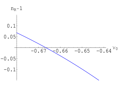
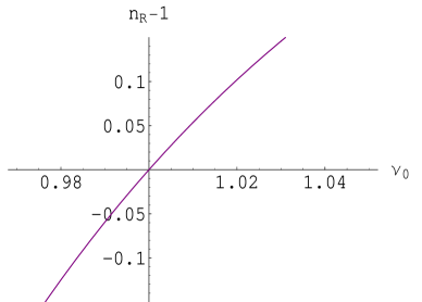
Figure 1: The index $n_{\cal R}-1$ as the function of $\nu_{0}$, with $V(\varphi)=0$ (cf equation 4.13); $n_{\cal R}$ does not vary much with the number of e-folds except that it is blue-tilted for $\Delta N\lesssim 0$. Even though $\nu_{0}<0$ generally implies a super-luminal inflation, it is possible to achieve a red-tilted spectrum for $\nu_{0}>-2/3$.

The constraint on the spectral indices might give a stringent bound on the scalar-Gauss-Bonnet coupling $f(\varphi)$, or the GB density fraction, $\Omega_{GB}$. The scalar index satisfies the bounds provided by the recent WMAP results, namely $n_{\cal R}=0.958_{-0.018}^{+0.014}$, for both signs of $\nu$, but in a limited range, see Fig. 1. In the $V(\varphi)=0$ case, in order to end inflation the function $\nu(\varphi)$ could be modified in a suitable way; in the case $mN<0$, implying that $\nu(\varphi)$ decreases with $N$, inflation ends naturally. With this particular example, we do not wish to imply that the model with a vanishing potential alone is compatible with recent data. Such a model may suffer from one or more (quantum) instabilities at short distance scales and/or local GR constraints [27] once the model is coupled to matter fields. As in  [36], we find that a model with $V(\varphi)>0$ is phenomenologically more viable than with $V(\varphi)=0$.

As noted above, a super-luminal expansion may occur if $\nu_{0}<0$, which corresponds to the case $\delta<0$ studied before in [15]. However, unlike claimed there, we find that it is possible to get a cosmic inflation of an arbitrary magnitude without violating the (null energy) condition $\dot{H}/H^{2}\leq 0$. For the solution (50), this simply required $\nu_{0}>0$; the Hubble rate would decrease with $N$. For $\nu_{0}<0$, one gets $\dot{H}/H^{2}>0$, especially, when ${\Delta N}\gtrsim 0$. The precise value of redshift $z$ ($\equiv e^{\Delta N}-1$) with such a drastic change in the background evolution actually depends on the strength of the coupling $f(\varphi)$, or the time variation of $\varphi$.

4.3 Inflating with an exponential potential

Let us take the scalar potential of the form

$$V(\varphi)=V_{0}\,e^{-\,2\varphi/\varphi_{0}},$$ (53)

leaving $f(\varphi)$ unspecified. The system of autonomous equations is then described by

$$\frac{dy}{dN}=-2y\epsilon-\frac{2xy}{\varphi_{0}},$$ (54)

$$\frac{dx}{dN}=\frac{(1+\epsilon)(y-3)}{\gamma x}-\frac{2y}{\gamma\varphi_{0}}-\frac{(5+\epsilon)x}{2},$$ (55)

$$u=\frac{1}{x}-\frac{y}{3x}-\frac{\gamma x}{6}.$$ (56)

These equations admit the following de Sitter (fixed point) solution

$$x=0,\quad V=\Lambda_{0},\quad H=\sqrt{\frac{\Lambda_{0}}{3}},\quad u=u(\varphi),$$ (57)

which corresponds to the case of a cosmological constant term, for which $w=-1$. In the particular case that $u\propto x$, so that $u\equiv f_{,\,\varphi}H^{2}$ is varying (decreasing) being proportional to the kinetic term for $\varphi$, we find an explicit solution, which is given by

$$x=\varphi_{0}-\alpha\,\varphi_{0}\tanh\alpha(N+N_{\lower 2.0pt\hbox{$\scriptstyle 1$}}),\quad u=-\frac{\gamma x}{3},\quad\epsilon=\frac{2\gamma x^{2}\varphi_{0}-2x(6+\gamma x^{2})}{\varphi_{0}(6+\gamma x^{2})},$$ (58)

where $\alpha\equiv\sqrt{(\gamma\varphi_{0}^{2}-6)/\gamma\varphi_{0}^{2}}<1$ and $N_{\lower 2.0pt\hbox{$\scriptstyle 1$}}$ is an integration constant. This solution supports a transition from deceleration ($\epsilon<-1$) to acceleration ($\epsilon>-1$), but inflation has no exit. The model should be supplemented by an additional mechanism, allowing the field $\varphi$ to exit from inflation after $50-60$ e-folds of expansion (see a discussion below).

For a negligibly small kinetic term, $x\simeq 0$, we have $\Omega_{GB}\propto x^{2}\approx 0$, while for a slowly rolling $\varphi$, $\Omega_{GB}\neq 0$. This behaviour is seen also from our numerical solutions in the next section. The evolution of $\varphi$ is given by

$$\varphi=\int x\,dN=N\varphi_{0}-\varphi_{0}\,\ln\cosh\alpha(N+N_{\lower 2.0pt\hbox{$\scriptstyle 1$}})+{\rm const}.$$ (59)

The scale factor, as given by $a\propto\exp[\int H\,dt]\propto\exp\left[\int\exp[\int\epsilon\,dN]\,dt\right]$, is regular everywhere. The coupling $f(\varphi)\equiv\int[u(\varphi)/\varphi^{\prime}H^{2}]\,d\varphi$ is rather a complicated function of $\varphi$, which is generally a sum of exponential terms. But given the fact that $x\simeq$ const at late times, or when $|\alpha(N+N_{\lower 2.0pt\hbox{$\scriptstyle 1$}})|\gtrsim 2$, we get $f_{,\,\varphi}\propto e^{\,2\varphi/\varphi_{0}}$. It is not difficult to see that the special solution considered in [8] corresponds to this particular case. To see it concretely, take

$$f(\varphi)=f_{0}\,e^{2\varphi/\varphi_{0}},$$ (60)

or, equivalently $\varphi_{0}u^{\prime}-2u(\varphi_{0}\epsilon+x)=0$. For the solution (58) this last condition imposes the constraint $\gamma\varphi_{0}^{2}=6$ and hence

$$x=x_{0},\quad u=-\gamma x_{0}/3.$$ (61)

The choice made in [8] for $V(\varphi)$ and $f(\varphi)$ thus over-constrains the system unnecessarily.

Can the solution (58) be used for explaining early inflation? In order to answer this question concretely, one may wish to evaluate cosmological parameters such as $n_{\cal R}$ and $n_{T}$. We can get the value of $n_{\cal R}$ in the range $0.94\lesssim n_{\cal R}\lesssim 0.99$ by taking $9\lesssim\sqrt{\gamma}\varphi_{0}\lesssim 20$. In fact, $n_{\cal R}$ may exceed unity precisely when $\epsilon>0$, leading to a momentary violation of the null energy condition (cf figure 2 (left panel)). However, after a certain number of e-folds of expansion, the tensor modes or the gravitational waves damp away (cf figure 2 (right panel)), leading to the observationally consistent result $|n_{T}|\lesssim 0$ and $n_{\cal R}-1\lesssim 0$ - leading to slightly red-tilted spectra (cf figure 3).

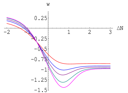
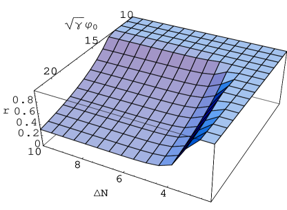
Figure 2: The left panel shows that the equation of state parameter $w$ that momentarily crosses the value $w=-1$. From top to bottom $\sqrt{\gamma}\varphi_{0}=4,5,6,8$ and $10$. The right panel shows the tensor-to-scalar ratio of cosmological perturbations; to adhere to the experimental constraint coming from recent WMAP results, namely $r<0.5$, one might require an almost flat potential, $\sqrt{\gamma}\varphi_{0}\gtrsim 16$.

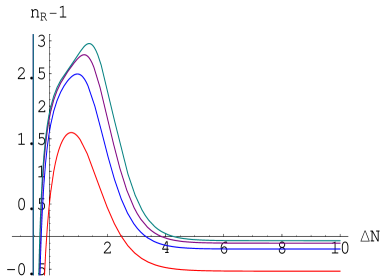
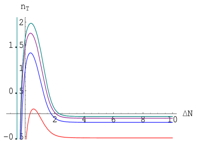
Figure 3: The spectral indices $n_{\cal R}-1$ and $n_{T}$ evaluated for the solution (4.21) by using the formulae given in (4.7); from top to bottom $\sqrt{\gamma}\varphi_{0}=10,8,6$ and $4$.

For the validity of (44), we require not only $\dot{\epsilon_{i}}\ll 1$ but also that the speed of propagation for scalars and tensor modes, $c_{k}^{2}$ and $c_{T}^{2}$, are nearly constant. This is however not the case for the above solution when $0\lesssim\Delta N\lesssim 3$, for which both $c_{r}^{2}$ and $c_{T}^{2}$ change rapidly. That means, the relations (44) must be modified in the regime where $c_{\cal R}^{2},c_{T}^{2}$ are varying. After a few number of e-folds of expansion, we have $c_{\cal R}^{2},c_{T}^{2}\simeq$ const. In this limit the spectral indices are found to be slightly red-tilted, i.e. $n_{\cal R}-1\lesssim 0$, for $\sqrt{\gamma}\varphi_{0}\gtrsim 8$.

A few remarks may be relevant before we proceed. The WMAP constraints on inflationary parameters that we referred to above, such as, the scalar index $n_{\cal R}$ and the tensor-to-scalar ratio $r$, are rather model dependent and may differ, for instance, for a model where the “inflaton” field is non-minimally coupled to gravity, or the spacetime curvature tensor. Hence, although those values may be taken as useful references, they may not be strictly applicable to all inflationary solutions driven by one or more scalar fields. In fact, some of our cases may have more freedom (less tight constraints) than the canonical models with a scalar potential proportional to $\varphi^{4}$ or $m_{\varphi}^{2}\varphi^{2}$, and $f(\varphi)=0$. We leave for future work the implications of WMAP data to scalar potentials of the form $V\propto H^{2}(\varphi)\varphi^{n}$ ($n\geq 2$).

4.4 Inflating with an exponential coupling

Let us take the scalar-GB coupling of the following form:

$$f_{,\varphi}=f_{0}\,e^{2\varphi/\varphi_{0}},$$ (62)

but without specifying the potential, $V(\varphi)$. With this choice, the system of monotonous equations is given by

$$\frac{du}{dN} = \frac{2(x+\epsilon\varphi_{0})}{\varphi_{0}}\,u,$$ (63)

$$\frac{dx}{dN} = \frac{2\epsilon+\gamma x^{2}}{u}+(1-3\epsilon)x-\frac{2x^{2}}{\varphi_{0}},$$ (64)

$$y = 3-\frac{\gamma}{2}\,x^{2}-3ux.$$ (65)

The de Sitter fixed point solution for which $x=0$ is the same as (57). In the following we consider two special cases:
(1) Suppose that $\mu\equiv{\rm const}$, that is, $\Omega_{GB}=$ const $\equiv\mu_{0}$. Then we find

$$\epsilon=\frac{\mu_{0}+\gamma x^{2}}{\mu_{0}-2},\quad\frac{dx}{dN}=\frac{2(\gamma\varphi_{0}x^{3}-(2-\mu_{0})x^{2}+2\mu_{0}\varphi_{0}x)}{(2-\mu_{0})\varphi_{0}}.$$ (66)

These equations may be solved analytically for $\mu_{0}=2/3$ ; as the solutions are still messy to write, we only show the behavior of $w$ in Mathematica plots. In the next section we will numerically solve the field equations, in the presence of matter, allowing us to consider all values of $\mu_{0}$. We should at least mention that the above system of equations has a pair of fixed point solutions:

$$x_{1}={2-\mu_{0}-\sqrt{(2-\mu_{0})^{2}-8\gamma\varphi_{0}\mu_{0}}\over 2\gamma\varphi_{0}},\quad x_{2}={2-\mu_{0}+\sqrt{(2-\mu_{0})^{2}-8\gamma\varphi_{0}\mu_{0}}\over 2\gamma\varphi_{0}}.$$ (67)

The fixed point $x_{1}$ is an attractor, while the $x_{2}$ is a repeller provided that $x_{1},x_{2}$ are real. In the case where $8\gamma\varphi_{0}\mu_{0}>(2-\mu_{0})^{2}$ the solution diverges. The solution also diverges for initial values of $x$ such that $x<0$ and $x>x_{2}$. If these conditions are not violated, the solutions would always converge to the attractor fixed point $x=x_{1}$. The evolution of the solution is monotonic from the initial value of $\epsilon$ to the $\epsilon$ given by the attractor fixed point at $x=x_{1}$. The initial value of $w$ for a wide range of $\mu_{0}$ and initial values of $x$ may be read from figure 4(a), and evolve to the $w$ given in figure 4(b) for a specific value of $\mu_{0}$.

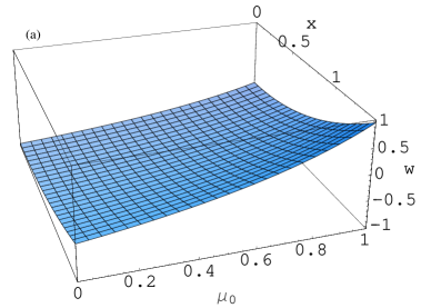
Figure 4: The left panel (a) shows the initial equation of state parameter ${\rm w}$ with various initial conditions for $\Omega_{GB}=\mu_{0}$ and $x$, while, the right panel (b) shows a possible variation of $w$ for a particular value of $\mu_{0}$; solutions evolve to these values regardless of $x_{ini}$ provided the fixed points exist and $0<x_{\rm ini}<x_{2}$. We have taken $\varphi_{0}^{-1}=2$ and $\gamma=1$

(2) Next suppose that $u=$ const $\equiv u_{0}$, instead of $ux=\mu$ =const. In this case, the quantity $x$ decreases quickly with the expansion of the universe; the GB density fraction, $\Omega_{GB}$, also decreases with the number of e-folds. The explicit solution is

$$\epsilon=-\frac{x}{\varphi_{0}},\qquad x=\frac{2-u_{0}\varphi_{0}}{\gamma\varphi_{0}+u_{0}+(2-u_{0}\varphi_{0})u_{1}\,e^{(2/u_{0}\varphi_{0}-1)N}},$$ (68)

where $u_{1}$ is an integration constant. Without any surprise, as $x\to 0$, $\epsilon\to 0$; the model then corresponds to the cosmological constant case.

Inflation is apparently future eternal for most solutions discussed above, e.g. (50) and (58). However, in a more viable cosmological scenario, the contribution of matter field may not be completely negligible. This is because, during inflation, the field $\phi$, while slowly evolving down its potential, which satisfies $\Delta\varphi\propto\Delta N$, decays into lighter particles and radiation. The inflaton may even decay to heavier particles, especially, if the reheating of the universe was due to an instance preheating [37]. In turn, a significant amount of the energy density in the $\varphi$ component might be transforming into the radiation and (baryonic plus dark) matter, with several hundreds of degrees of freedom and with all components present, e.g. stiff matter ($p=\rho$) and radiation ($3p=\rho$). In turn, the slow roll type parameter $\epsilon$ would receive a non-trivial contribution from the matter fields. Explicitly, we find

$$\epsilon=-\frac{3}{2}\,(1+w)\Omega_{\lower 2.0pt\hbox{$\scriptstyle b$}}-\frac{{\varphi^{\prime}}^{2}}{2},$$ (69)

where $\Omega_{b}=\Omega_{\lower 2.0pt\hbox{$\scriptstyle m$}}+\Omega_{\lower 2.0pt\hbox{$\scriptstyle r$}}$ and $w\equiv(p_{\lower 2.0pt\hbox{$\scriptstyle m$}}+p_{\lower 2.0pt\hbox{$\scriptstyle r$}})/(\rho_{\lower 2.0pt\hbox{$\scriptstyle m$}}+\rho_{\lower 2.0pt\hbox{$\scriptstyle r$}})$. Inflation ends when there is significant portion of matter fields, which makes $\epsilon$ more and more negative and hence $\epsilon<-1$.

Before proceeding to next section we also wish to make a clear separation between the inflationary solutions that we discussed above and the dark energy cosmologies that we will discuss in the following sections. Although it might be interesting to provide a natural link between the early universe inflation and the late time cosmic acceleration attributed to dark energy, postulating a string-inspired model of quintessential inflation, the time and energy scales involved in the gravitational dynamics may vastly differ. As we have seen, through the construction of potentials, the scalar potential driving an inflationary phase at early epoch and a second weak inflationary episode at late times could be due to a single exponential term or a sum of exponential terms, but the slopes of the potential of the leading terms could be very different. In fact, one of the very interesting features of an exponential potential is that the cosmological evolution puts stringent constraints, e.g. during big-bang nucleosynthesis, on the slope of the potential, but its coefficient may not be tightly constrained. That is, even if we use the potential $V(\varphi)=V_{0}\,e^{-\beta\varphi}$, with $\beta\sim{\cal O}(1-10)$, for explaining both the early and the late time cosmic accelerations, the magnitude of the coefficient $V_{0}$ can be significantly different, hence indicating completely different time and energy scales.

5 When matter fields are present

The above results were found in the absence of radiation and matter fields. It is thus natural to ask what happens in a more realistic situation, at late times, when both radiation and matter evolve together with the field $\varphi$. In such cases a number of new and interesting background evolutions might be possible. Also some of the pathological features, like the appearance of super-luminal scalar modes, may be absent due to non-trivial scalar-matter couplings.

5.1 Minimally coupled scalar field

We shall first consider the case of a minimal coupling between $\varphi$ and the matter, so $A(\varphi)=1$. Then, equations (4)-(6) and (10) can be easily expressed as a system of three independent equations. After a simple calculation, we find

$$\epsilon=-\frac{1}{2}\left(\ln\Omega_{b}\right)^{\prime}-\frac{3}{2}(1+w_{b}),$$ (70)

$$\mu^{\prime}=3(1+w_{b}\Omega_{b})+2\epsilon+\frac{\gamma x^{2}}{2}-y-(2+\epsilon)\mu,$$ (71)

subject to the constraint $\Omega_{\varphi}+\Omega_{GB}+\Omega_{b}=1$. Note that the background equation of state parameter $w_{b}$ is a function of $N$, not a constant. One can write $w_{b}\Omega_{b}=w_{m}\Omega_{m}^{(d)}+w_{m}^{(s)}\Omega_{m}^{(s)}+w_{r}\Omega_{r}$, so that $w_{m}=0$ and $w_{r}=1/3$ for pressureless dust and radiation, respectively, while for a relativistic fluid, e.g. hot and warm dark matter, we have $w_{m}^{(s)}>0$. In fact, the first equation above, (70), gives the condition for accelerated expansion, which requires $\epsilon>-1$. There are two ways to interpret this equation: either it gives $w_{\rm eff}$ in terms of $w_{b}$, assuming that the ratio $\Omega_{b}^{\prime}/\Omega_{b}$ is known, or it provides for fixed $w_{b}$ the value of $w_{\rm eff}$ that may be related to the ratio $\Omega_{b}^{\prime}/\Omega_{b}$. Of course, in the absence of kinetic term for $\varphi$ (so $x=0$), $f(\varphi)$ is uniquely fixed once $V(\varphi)$ is chosen. Such a construction is however not very physical.

An interesting question to ask is: What is the advantage of introducing a non-trivial coupling $f(\varphi)$, if it only modifies the potential or the variable $y$, without modifying the functional relation between $\epsilon$ and $\Omega_{b}$? For the model under consideration without such a coupling there does not exist a cosmological solution crossing the phantom divide, $w=-1$.

As a very good late time approximation, suppose that the ratio $\dot{\varphi}/H$ takes an almost constant value, say $\beta$, rather than $\dot{\varphi}=0$, along with $H\propto\,e^{-\,\lambda\phi/2}$, where $\phi\equiv\sqrt{\gamma}\,(\varphi-\varphi_{0})/{\beta}=N$. The background matter density fraction is then given by

$$\Omega_{b}=\Omega_{0}\,\exp[\lambda\phi-3(1+w_{b})\phi],$$ (72)

where $\Omega_{0}\equiv c_{1}\,(6w_{b}+8-\lambda)/[3(2-\lambda)]$. For $\lambda<2$, the physical choice is $c_{1}>0$, so that $\Omega_{b}>0$. The scalar potential and the GB density fraction evolve as

$$V = \frac{3(2-\lambda)+\beta^{2}(5-\lambda/2)}{2+\lambda}\,e^{-\,\lambda\phi}-c_{1}\,e^{-\,3(1+w_{b})\phi}+c_{2}\,e^{\,\lambda\phi/2},$$ (73)

$$\Omega_{GB} \equiv \mu=\frac{2(\lambda-\beta^{2})}{2+\lambda}-\frac{c_{1}(1+w_{b})}{2-\lambda}\,e^{\lambda\phi-3(1+w_{b})\phi}-\frac{c_{2}}{3}\,e^{(2+\lambda)\phi/2},$$ (74)

where $c_{1},c_{2}$ are integration constants. The second term in each expression indicates a non-trivial contribution of the background matter and radiation. The presence of $c_{1}$ term in (73) implies that the value of the density fraction $\Omega_{b}$ must be known rather precisely for an accurate reconstruction of the potential. Equation (74) implies that

$$f(\varphi)\equiv f_{0}\,{\rm e}^{\lambda\phi}+f_{1}\,e^{2\lambda\phi-3(1+w_{b})\phi}-f_{2}\,e^{(2+\lambda/2)\phi},$$ (75)

where $f_{1}$ and $f_{2}$ take, respectively, the signs of $c_{1}$ and $c_{2}$. If $V$ is sufficiently flat near the current value of $\varphi$, then both the background and Gauss-Bonnet density fractions, $\Omega_{b}$ and $\Omega_{GB}$, may take nearly constant values. At late times, $w_{b}\simeq w_{m}\simeq 0$ for the pressureless dust, while the radiation contribution may be neglected since $\Omega_{r}\sim 10^{-4}$.

5.2 Non-minimally coupled scalar field

To investigate a possible post-inflation scenario, where the scalar field may couple non-minimally to a relativistic fluid or stiff-matter other than to ordinary matter or dust, we consider the following three different epochs: (1) background domination by a stiff relativistic fluid, (2) radiation domination and (3) a relatively long period of dust-like matter domination which occurred just before the current epoch of dark energy or scalar field domination. To this end, we define the fractional densities as follows: $\Omega_{s}$ for stiff-matter, $\Omega_{r}$ for radiation and $\Omega_{d}$ for dust, where the respective equation of state parameters are given by $w_{s}=1$, $w_{r}=1/3$ and $w_{d}=0$. Equations (12)-(14) may be written as

$$\Omega_{s}^{\prime}+2\epsilon\Omega_{s}+3\Omega_{s}(1+w_{s}) = -3\eta_{s}Q_{s}\Omega_{s}\varphi^{\prime},$$ (76)

$$\Omega_{d}^{\prime}+2\epsilon\Omega_{d}+3\Omega_{d} = -3Q_{d}\Omega_{d}\varphi^{\prime}.$$ (77)

$$\Omega_{r}^{\prime}+2\epsilon\Omega_{r}+4\Omega_{r} = 0,$$ (78)

In order for current experimental limits on verification of the equivalence principle to be satisfied, the coupling must be small, $Q_{d}^{2}\ll 1$, at present, see e.g. [22].

Superstring theory in its Hagedorn phase (a hot gas of strings), and also some brane models, naturally predict a universe filled with radiation and stiff-matter. To this end, it is not unreasonable to expect a non-trivial coupling of the field $\varphi$ with the stiff-matter: highly relativistic fluids may have strong couplings of the order of unity, $Q_{s}\sim{\cal O}(1)$. More specifically, as we do not observe a highly relativistic stiff-matter at the present time, i.e. $\Omega_{s}\approx 0$, the scalar-stiff-matter coupling $Q_{s}$ in the order of unity is not ruled out and may have a quantifiable effect on the evolution of the early universe.

5.3 The $\Omega_{GB}=$ const solution

It is interesting to study the case of a constant $\Omega_{GB}$ as it allows us to evolve the potential without constraining it through an ansatz. An exponential potential is generally used in the literature due to the simplification it affords allowing a change of variables and hence a system of autonomous equations.

It is worthwhile to investigate whether a physically interesting result can be found without the need for an ansatz for the potential. To this end, let us take $\Omega_{GB}\simeq{\rm const}\equiv\mu_{0}$. With the ansatz (62), we have

$$\frac{{\rm d}x}{{\rm d}N}=-2x(\epsilon+{x\over\varphi_{0}})$$ (79)

$$y=3-{\gamma\over 2}x^{2}-3\mu_{0}-3(\Omega_{r}+\Omega_{s}+\Omega_{d}),$$ (80)

where

$$\epsilon=\frac{\gamma x^{2}+\mu_{0}+2x(\eta_{s}Q_{s}\Omega_{s}+\eta_{d}Q_{d}\Omega_{d})+3\Omega_{r}(1+w_{r})+3\Omega_{s}(1+w_{s})+3\Omega_{d}(1+w_{d})}{\mu_{0}-2},$$ (81)

in addition to the continuity equations (76)-(78) describing the system. We also note that, since $\epsilon=H^{\prime}/H$, $H$ is solved from equation (81), allowing us to find both the scalar field potential $V=yH^{2}$ and the effective potential $\Lambda(\varphi)\equiv V(\varphi)+3f(\varphi)H^{4}(1+\epsilon)$ explicitly. We can see that there is a strong correlation between the length of dust-like matter domination and the parameter values, $\mu_{0}$ and $\Omega_{d,\rm ini}$.

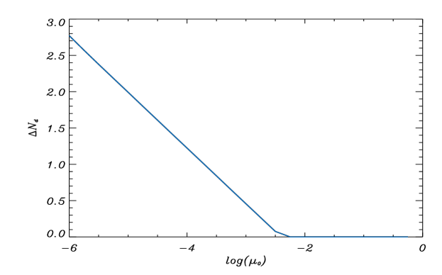
Figure 5: The period of dust-like matter domination as a function of $\mu_{0}$ for $f_{,\varphi}=f_{0}\,e^{3\varphi}$, $\gamma=1$, $Q^{2}_{d}=10^{-5}$ and $Q^{2}_{s}=0.01$. The initial conditions are $x=10^{-7}$, $y=10^{-15}$, $\Omega_{d}=0.1$ and $\Omega_{r}=0.45$.

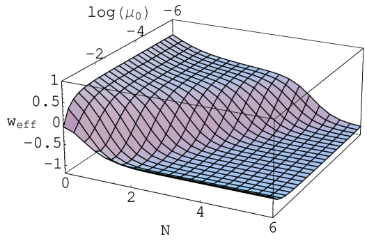
Figure 6: The behaviour of $w_{\rm eff}$ for varying $\mu_{0}$ for $f_{,\varphi}=f_{0}\,e^{3\varphi}$, $\gamma=1$, $Q^{2}_{d}=10^{-5}$ and $Q^{2}_{s}=0.01$. The initial conditions are $x=10^{-7}$, $y=10^{-15}$, $\Omega_{d}=0.1$ and $\Omega_{r}=0.45$.

The dust domination period is expected to last for about $5-7$ e-folds of expansion. However, in the above case, no parameter ranges meet this condition while still maintaining a (relatively) long period of radiation domination. This is problematic as at least some period of radiation domination appears to be a requirement for reconciling any cosmological model with observations. Our results here are therefore presented in the spirit of a toy model, which allow the evolution of an unconstrained potential for parameter ranges and give solutions with the expected qualitative features.

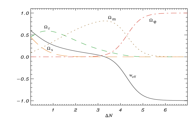
Figure 7: The evolution of the fractional densities and $w_{\rm eff}$ (solid line, black) for a fixed $\mu_{0}=10^{-6}$ with parameters $\gamma=1$, $\varphi_{0}=2/3$, $Q^{2}_{d}=10^{-5}$ and $Q^{2}_{s}=0.01$, and initial conditions as $x=10^{-7}$, $y=10^{-15}$, $\Omega_{d}=0.1$ (dots, brown) and $\Omega_{r}=0.45$ (dashes, green). $\Omega_{s}$ is represented by long dashes (orange) and $\Omega_{\varphi}$ by dot-dash (red).

Figure 8: The left panel shows the evolution of $V(\varphi)$ while the right panel shows the evolution of $V_{\rm eff}\equiv V(\varphi)+3f(\varphi)H^{4}(1+\epsilon)$ for $\mu_{0}=10^{-6}$, $\gamma=1$, $f(\varphi)\propto e^{3\varphi}$, $Q^{2}_{d}=10^{-5}$ and $Q^{2}_{s}=0.01$ with initial conditions $x=10^{-7}$, $y=10^{-15}$, $\Omega_{d}=0.1$, $\Omega_{r}=0.45$, $H=0.01$ and $f(\varphi)_{\lower 2.0pt\hbox{$\scriptstyle\rm ini$}}=10^{-10}$.

Figure 5 shows the period of dust domination observed for various values of $\mu_{0}$. We see that, in the parameter range $\mu_{0}\lesssim 10^{-3}$, there exist solutions supporting both radiation and stiff-matter domination prior to matter domination. While for larger values of $\mu_{0}$ the Gauss-Bonnet contribution suppresses the background fields and we may observe a quick transition to scalar-field domination, missing either the radiation dominated era or the matter dominated era, or both. For smaller values of $\mu_{0}$, no solutions exist for the parameters used above due to constraints in the field equations. The behaviour of $w_{\rm eff}$ for varying $\mu_{0}$ and the general evolution of the cosmology are shown in figure 6 and figure 7, respectively. In the cases where the second derivative of $w_{\rm eff}$ is monotonic there is no radiation domination ($w_{\rm eff}\sim 1/3$) or dust domination ($w_{\rm eff}\sim 0$). For lower values of $\mu_{0}$, the second derivative of $w_{\rm eff}$ obviously changes sign and hence implies a period of background matter or radiation domination. We show the behaviour of the scalar potential and the corresponding effective potential in figure 8.

5.4 Simplest exponential potentials

We now wish to consider the evolution of the full system while putting minimal restrictions on the evolution of the cosmological constituents. To do this we employ simple single exponential terms for both the field potential and the scalar-GB coupling:

$$f_{,\varphi}(\varphi)=f_{0}\,e^{\alpha\varphi}\hskip 17.07182pt{\rm and}\hskip 17.07182ptV(\varphi)=V_{0}\,e^{-\beta\varphi}.$$ (82)

The commonly invoked exponential potential ansatz has some physical motivation in supergravity and superstring theories as it could arise due to some nonperturbative effects, such as gaugino condensation and instantons. One can see that these choices are almost undoubtedly too naive to allow all the expected physical features of our universe from inflation to the present day. This is because generally the slopes of the potential considered in post-inflation scenarios are too steep to allow the required number of e-folds of inflation in the early universe. As a post-inflation approximation, however, these may hold some validity, as one can replicate many observable physical features from nucleosynthesis to the present epoch while allowing non-trivial scalar-matter couplings. In follow-up work we will discuss the possibility of a two-scalar fields model where the potential related to one scalar field meets the requirements of inflation while the other scalar drives the late time cosmology.

The ansätze (82) allow us to write an autonomous system

$$\quad{{\rm d}x\over{\rm d}N} = -{1\over 2\gamma}\big{[}2\gamma x\epsilon+6\gamma x-2\beta y+6u(1+\epsilon)-6\eta_{s}Q_{s}\Omega_{s}$$ (83)

$$\quad+\eta_{d}Q_{d}\{\gamma x^{2}+2y+6(ux+\Omega_{r}+\Omega_{s}-1)\}\big{]}$$

$${{\rm d}y\over{\rm d}N} = -y(\beta x+2\epsilon)$$ (84)

$${{\rm d}u\over{\rm d}N} = u(\alpha x+2\epsilon)$$ (85)

where

$$\hskip 14.22636pt\epsilon = \frac{1}{6(2\gamma ux-2\gamma-3u^{2})}\bigg{[}18\gamma\left(1+w_{d}-w_{d}\Omega_{r}-w_{d}\Omega_{s}+w_{r}\Omega_{r}+w_{s}\Omega_{s}\right)$$ (86)

$$+6\gamma ux-6\gamma y+3\gamma^{2}x^{2}+18u^{2}-3\gamma^{2}w_{d}x^{2}-6\beta uy-6\gamma\alpha ux^{2}-18\gamma w_{d}ux-6\gamma w_{d}y$$

$$-\eta_{d}Q_{d}(2\gamma^{2}x^{3}+18u-18u^{2}x-6uy-18u\Omega_{r}-12\gamma x+4\gamma xy+12\gamma x\Omega_{r}+9\gamma ux^{2})$$

$$-\left(\eta_{d}Q_{d}-\eta_{s}Q_{s}\right)\left(12\gamma x-18u\Omega_{s}\right)\bigg{]},$$

which along with the continuity equations (76)-(78) and the Friedmann constraint equation, $\Omega_{d}+\Omega_{\varphi}+\Omega_{GB}+\Omega_{r}+\Omega_{s}=1$, allow us to proceed with numerical computation.

We look particularly at two values for $\beta$ here, $\beta=\sqrt{2/3}$ and $\beta=\sqrt{3}$, while keeping the other parameters constant to limit the vast parameter space. These values may be motivated by various schemes of string or M theory compactifications (see, e.g. [30]). We will discuss the effects of varying these other parameters and some of the physically relevant results. The evolution of the various constituents is shown in figures 9-10.

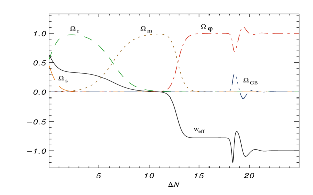
Figure 9: Evolution of the fractional densities and $w_{\rm eff}$ (solid line, black) where $\beta=\sqrt{2/3}$, $\gamma=1$, $\alpha=12$, $Q_{d}^{2}={10}^{-5}$ and $Q_{s}^{2}=0.01$ with initial conditions $x=\sqrt{6}\times 10^{-4}$, $y=5\times 10^{-20}$, $u=0.08$, $\Omega_{r}=0.549$ (dashes, green) and $\Omega_{s}=0.45$ (long dashes, orange). $\Omega_{d}$ is represented by dots (brown), $\Omega_{\varphi}$ by dot-dash (red) and $\Omega_{GB}$ by dot-dot-dot-dash (blue).

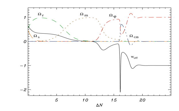
Figure 10: Evolution of the fractional densities and $w_{\rm eff}$ (solid line, black) where $\beta=\sqrt{3}$, $\gamma=1$, $\alpha=12$, $Q_{d}^{2}={10}^{-5}$ and $Q_{s}^{2}=0.01$ with initial conditions $x=\sqrt{6}\times 10^{-4}$, $y=5\times 10^{-20}$, $u=0.08$, $\Omega_{r}=0.549$ (dashes, green) and $\Omega_{s}=0.45$ (long dashes, orange). $\Omega_{d}$ is represented by dots (brown) and $\Omega_{\varphi}$ by dot-dash (red), $\Omega_{GB}$ by dot-dot-dot-dash (blue).

The $\beta=\sqrt{2/3}$ case appears to show a smoother evolution and has a short period during which there is acceleration and an appreciable amount of matter in the universe. In the table below we look at some of the features of the accelerating period for the solution given in figure 9. At the onset of acceleration, $w_{\rm eff}=-1/3$, we have $\Omega_{d}=0.650$. Within the best-fit concordance cosmology the present observational data seem to require $w_{\rm eff}<-0.74$ [39]. However, in the above case, this requires less matter ($\Omega_{d}\lesssim 0.12$) than in $\Lambda$CDM model.

Condition imposed at present	$\Delta N_{\rm accelerating}$	Implied $w_{\rm eff}$	Implied $\Omega_{d}$
$\Omega_{d}=0.27$	$0.582$	$-\,0.648$	N/A
$w_{\rm eff}=-\,0.74$	$0.955$	N/A	$0.123$
$w_{\rm eff}=-\,0.9$	$5.48$	N/A	$3.02\times 10^{-6}$
$w_{\rm eff}=-\,1.0$	$5.55$	N/A	$2.46\times 10^{-6}$
$\Delta N=0.69$	N/A	$-\,0.685$	$0.215$
$\Delta N=0.91$	N/A	$-\,0.734$	$0.134$

The recent type Ia supernovae observations [40] appear to indicate that the universe may be accelerating out to a redshift of $z\sim 0.4-1$ [41]. In terms of the number of e-folds of expansion, this corresponds to $\Delta N=\ln(1+z)\sim 0.34-0.69$, if one assumes a rescaling of $N\rightarrow 0$ at the present epoch using the freedom in choosing the initial value of the scale factor, $a_{0}$. We have chosen the initial value of $y$, or the ratio $V(\varphi)/H^{2}$, such that the period of dust-like matter domination is $\Delta N_{\Omega_{d}}\sim 6.5$ as this corresponds to a total redshift of $z\sim 1100$ to the epoch of matter-radiation equality.

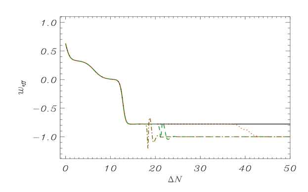
Figure 11: Evolution of $w_{\rm eff}$ with $\beta=\sqrt{2/3}$, $\gamma=1$, $Q_{d}^{2}=10^{-5}$ and $Q_{s}^{2}=0.01$; $\alpha=12$ (dash-dot, brown), $8$ (dashes, green), $3$ (dots, red), $\sqrt{2/3}$ (solid, black), with initial values $x=\sqrt{6}\times 10^{-4}$, $y=5\times 10^{-20}$, $u=0.08$, $\Omega_{r}=0.549$ and $\Omega_{s}=0.45$.

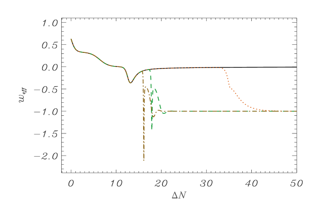
Figure 12: Evolution of ${\rm w}_{\rm eff}$ with $\beta=\sqrt{3}$, $\gamma=1$, $Q_{d}^{2}=10^{-5}$ and $Q_{s}^{2}=0.01$; $\alpha=12$ (dash-dot, brown), $8$ (dashes, green), $3$ (dots, red), $\sqrt{2/3}$ (solid, black), with initial values $x=\sqrt{6}\times 10^{-4}$, $y=5\times 10^{-20}$, $u=0.08$, $\Omega_{r}=0.549$ and $\Omega_{s}=0.45$.

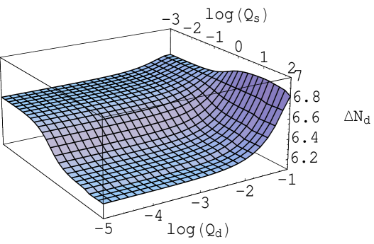
Figure 13: The period of dust-like matter domination for varying $Q_{s}$ and $Q_{d}$ for $\gamma=1$, $\alpha=12$ and $\beta=\sqrt{2/3}$ with initial conditions $x=\sqrt{6}\times 10^{-5}$, $y=5\times 10^{-20}$, $u=0.08$, $\Omega_{r}=0.549$ and $\Omega_{s}=0.45$.

Figure 14: Evolution of $w_{\rm eff}$ for different values of $Q_{s}$: $Q_{s}^{2}=10^{4}$ (dots, green) $100$ (dashes, orange), $0$ (solid, black) and $1$ (dash-dot, red) with fixed $Q_{d}=\sqrt{10^{-5}}$ and $\gamma=1$, $\alpha=12$, $\beta=\sqrt{2/3}$. The initial conditions are $x=\sqrt{6}\times 10^{-4}$, $y=5\times 10^{-20}$, $u=0.1$, $\Omega_{r}=0.549$ and $\Omega_{s}=0.45$. The larger, more violent oscillations seen for $Q_{s}>1$ are due to significant scalar-stiff-matter couplings, while the smooth oscillations for smaller couplings at some later stage are due to an appreciable contribution of the coupled Gauss-Bonnet term.

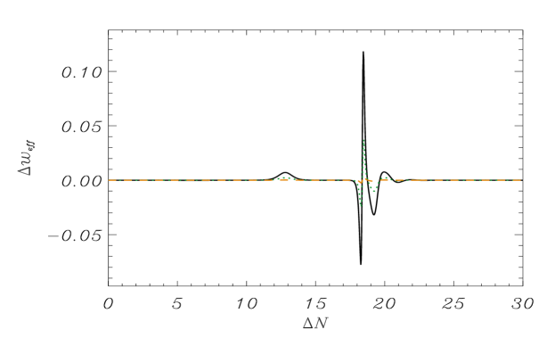
Figure 15: Variation of $w_{\rm eff}$ for non-zero $Q_{d}$ as compared to the $Q_{d}=0$ case, $\Delta w_{\rm eff}\equiv w_{\rm eff}(Q_{d}\neq 0)-w_{\rm eff}(Q_{d}=0)$; $Q_{d}^{2}=10^{-5}$ (solid, black), $10^{-6}$ (dots, green) and $10^{-8}$ (dashes, orange) and $Q_{s}=0.1$. Clearly, for higher values of the scalar dust-matter couplings, $Q_{d}^{2}>{10}^{-5}$, we find slightly larger variations in $w_{\rm eff}$.

The evolution with $\beta=\sqrt{3}$ does not seem to be in favourable agreement with current cosmological observations. The solution may undergo a period of sudden change in $w_{\rm eff}$ when the Gauss-Bonnet contribution becomes appreciable (or significant); this would have to occur around at the present epoch as to retrieve the current value of $w_{eff}\sim-1$. This result does not reconcile with either the supernovae data, which seem to indicate a longer period of acceleration, or with a constraint for the present value of Gauss-Bonnet density [27] which may require that $\Omega_{GB}\lesssim 0.2$, or with the presently anticipated value of $\Omega_{d}$ ($\sim 0.27$).

We can observe an oscillatory crossing of $w_{\rm eff}=-1$ limit for all cases in which the Gauss-Bonnet contribution becomes appreciable, even momentarily. Such a behaviour may be seen in variants of scalar-tensor models [42]. In our case, the amplitude of these oscillations corresponds to the amplitude of the oscillations seen in the Gauss-Bonnet contribution and hence is heavily dependent on the slope of the scalar-GB coupling; for large $\alpha$ we observe much larger oscillations. These oscillations damp quickly as the Gauss-Bonnet contribution becomes negligibly small, and settle to a late time evolution for which $w_{\rm eff}\approx-1$. As this limit is approached from above, none of the issues inherent with super-inflation or a violation of unitarity will be applicable to the late time cosmology.

As the parameter space for the initial conditions is very large we have presented solutions with initial conditions and parameters selected to give reasonable periods of radiation and dust-like matter domination as well as other physically favourable features. Although the quantitative behaviour is observed to change smoothly with changes in initial conditions and parameters, such changes do have some qualitative effects as limits of certain behaviour are encountered. A quantitative variation in the period of dust-like matter domination can be attributed to altering the initial value of $y$ or $\Omega_{d,\rm ini}$; lower values of $y_{\rm ini}$ extend the period before scalar field domination begins. This is effectively a change in the initial potential and has a monotonic effect on the epoch at which scalar field domination begins. In a qualitative sense, it has no effect on the period of radiation domination until a $y_{\rm ini}$ is selected which is large enough that the scalar field contribution completely suppresses the dust-like matter domination period. The value of $\Omega_{d,\rm ini}$ is relevant to the epoch of matter-radiation equality, larger values result in an earlier epoch. For small values, no dust-like matter domination occurs and the solution is entirely dominated by the other four constituents considered. The limits at which all these effects occur are dependent on other parameters and hence discussion of actual values instead of the general behaviour does not add further insight.

We note that the exponential terms for both the potential and the coupling have some noticeable effects on the evolution of the system. This may be seen to an extent in terms of $\beta$ in figures 9-12. It does, however, appear that the ratio of these parameters also influences the expansion during dust-like matter domination remaining, relatively unchanged when this ratio is constant within realistic $\beta$ and $\alpha$ parameter ranges. Phenomenological bounds on these values have been studied in [20].

For $\alpha\sim\beta$ we do not observe a significant period of Gauss-Bonnet contribution and hence no crossing of the $w_{\rm eff}=-1$ limit. The closer the value of $\alpha$ is to this limit the later this period of significant Gauss-Bonnet density fraction occurs. As $\alpha$ increases there is a minimum epoch at which the Gauss-Bonnet contribution becomes significant, this epoch occurs after the scalar field becomes the dominant component in the energy budget of our universe. Results for various values of $\alpha$ are shown in figures 11 and 12.

The consequences of matter coupling to the scalar field on the cosmology are of particular interest. The effect in the period of dust-like matter-domination is minimal in relation to both $Q_{d}$ and $Q_{s}$ and can be seen in figure 13, though we allowed the value $Q_{s}\gg Q_{d}$. As there is a lack of observational or theoretical motivation refuting the possibility of a high relativistic-matter-scalar coupling we consider a range that extends beyond $Q_{s}=1$ whereas the dust-like-matter-scalar coupling must take values $Q_{d}^{2}<10^{-5}$ due to the current level of experimental verification in solar system tests of GR.

The solution undergoes a transition in qualitative behaviour when we extend through the limit $Q_{s,\rm lim}\sim 1$, where the exact onset and amplitude of its effects are dependent on the other parameter values taken. Hence our remarks again apply to the general behaviour observed rather than specific cases. Couplings greater than $Q_{s,\rm lim}$ cause a non-negligible reemergence of the stiff-matter contribution at the end of dust-like matter domination. The density fraction of the relativistic matter undergoes a damped oscillations, generally with a much shorter period of oscillation than the oscillations observed in the non-negligible Gauss-Bonnet contribution. This causes corresponding oscillations in the effective EoS, while still generally showing the same overall trend as for lower $Q_{s}$ values of the otherwise same solution, with the density fraction of the relativistic matter stabilising to a non-zero late time value. This cosmological behaviour does not appear to be physically valid as no mechanism to generate this relativistic matter seems plausible and would hence lead us to suggest that the value of $Q_{s}$ would have an upper-bound such that $Q_{s,\rm max}\sim Q_{s,\rm lim}$. The effects of $Q_{s}$ and $Q_{d}$ on the effective equation of state parameter, $w_{\rm eff}$, may be seen in figures 14 and 15. Note that in figure 15 we have considered $\Delta w_{eff}$ rather than $w_{eff}$ as the effects of varying $Q_{d}$ are so minimal that no discernable variation can be seen otherwise. In these figures we have considered the same solutions as in figure 9. The magnitude of the effects are, however, the same throughout the parameter space.

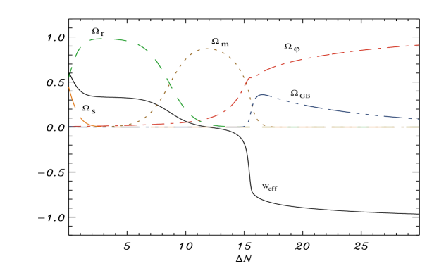
Figure 16: Evolution of the fractional densities and $w_{\rm eff}$ (solid line, black) for the potential ansatz $V(\varphi)=H^{2}(\Lambda_{0}+\Lambda_{1}e^{-\beta\varphi})$ where $\gamma=1$, $\alpha=9$, $\beta=\sqrt{2/3}$, $\Lambda_{0}=10^{-8}$, $Q_{d}^{2}={10}^{-5}$ and $Q_{s}^{2}=0.01$ with initial conditions $x=\sqrt{6}\times 10^{-2}$, $y=9\times 10^{-3}$, $u=0.1$, $\Omega_{r}=0.549$ and $\Omega_{d}=10^{-4}$. $\Omega_{\rm r}$ is represented by dashes (green), $\Omega_{\rm d}$ by dots (brown) $\Omega_{s}$ by long dashes (orange), $\Omega_{\varphi}$ by dot-dash (red) and $\Omega_{GB}$ by dot-dot-dot-dash (blue).

5.5 A canonical potential

Motivated by our results in section 3, we consider the potential

$$V(\varphi)=H^{2}(\Lambda_{0}+\Lambda_{1}e^{\beta\varphi}).$$ (87)

Imposing this ansatz along with the scalar-GB coupling given in equation (82), $f(\varphi)\propto e^{\alpha\varphi}$, allows us to find solutions that have reasonable agreement with concurrent observations while not crossing the $w_{\rm eff}=-1$ limit at any stage of the evolution. From figure (16) we can see that the cosmic evolution shows a smooth progression to $w_{\rm eff}=-1$, which may be physically more sensible. The amplitude of the Gauss-Bonnet density fraction at maximum is dependent on the values of slope $\alpha$, for smaller $\alpha$ it never becomes relevant. The period of dust-like matter domination again shows a heavy dependence on the initial value of $y$ or the potential $V(\varphi)$.

Here we also make an essential remark related to all our numerical plots in sections $5$ and $6$. Taking into account the relation $\Delta N\equiv\ln(1+z)$, one may (incorrectly) find that the present epoch corresponds to $\Delta N\sim 15$. However, in our numerical analysis, we are interested in the general evolution of the universe, in terms of the e-folding time $N\equiv\ln[a(t)]$, from the (early) epoch of radiation-dominated universe to the present epoch. Indeed, our solutions are completely invariant under a constant shift in $\Delta N$, so the choice of $N_{\lower 2.0pt\hbox{$\scriptstyle 0$}}$ in $\Delta N=N+N_{\lower 2.0pt\hbox{$\scriptstyle 0$}}$ is arbitrary. One may choose $N_{\lower 2.0pt\hbox{$\scriptstyle 0$}}$ such that $\Omega_{\lower 2.0pt\hbox{$\scriptstyle m$}}\simeq 0.27$ at present, or alternatively $N_{\lower 2.0pt\hbox{$\scriptstyle 0$}}\sim 15$, so that $a_{\lower 2.0pt\hbox{$\scriptstyle 0$}}=1$ (the present value of the scale factor) corresponds to $N\simeq 0$.

6 Remarks on ghost conditions

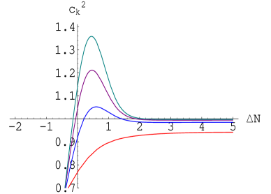
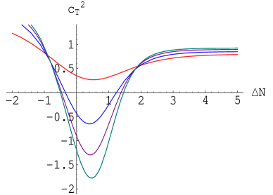
Figure 17: The speeds of propagation for scalar and tensor modes, corresponding to the solution (4.21) with $\sqrt{\gamma}\varphi_{0}=3,4,5$ and $6$ from top to bottom (bottom to top) for the left (right) panel.

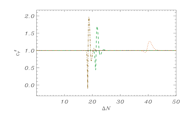
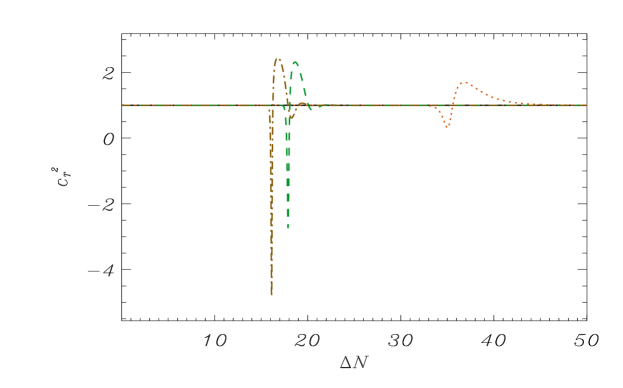
Figure 18: The variation of $c_{T}^{2}$ with $\Delta N$; (top panel) $\beta=\sqrt{2/3}$ and $\alpha=12\,{\rm(dash-dot,brown)},\,8\,{\rm(dashes,green)},\,3\,{\rm(dots,orange)},\,\sqrt{2/3}\,{\rm(solid,black)}$; (bottom panel) $\beta=\sqrt{3}$ and $\alpha=12\,{\rm(dash-dot,brown)},\,8\,{\rm(dashes,green)},\,3\,{\rm(dots,orange)},\,\sqrt{2/3}\,{\rm(solid,black)}$. Other parameters are chosen as $\gamma=1$, $Q_{d}^{2}=10^{-5}$ and $Q_{s}^{2}=0.01$, with initial conditions $x=\sqrt{6}\times 10^{-4}$, $y=5\times 10^{-20}$, $u=0.08$, $\Omega_{r}=0.549$ and $\Omega_{s}=0.45$.

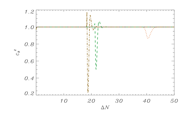
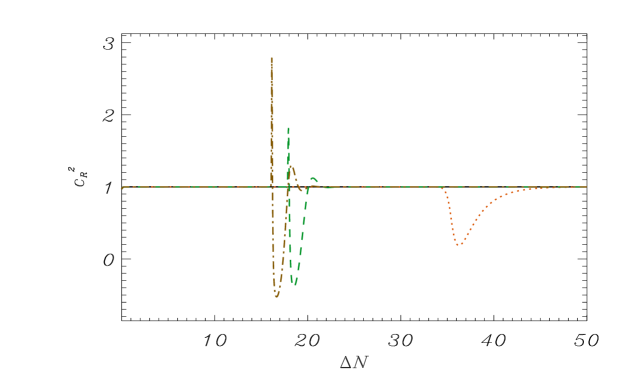
Figure 19: The variation of $c_{{\cal R}}^{2}$ with $\Delta N$; (top panel) $\beta=\sqrt{2/3}$ and $\alpha=12\,{\rm(dash-dot,brown)},\,8\,{\rm(dashes,green)},\,3\,{\rm(dots,orange)},\,\sqrt{2/3}\,{\rm(solid,black)}$; (bottom panel) $\beta=\sqrt{3}$ and $\alpha=12\,{\rm(dash-dot,brown)},\,8\,{\rm(dashes,green)},\,3\,{\rm(dots,orange)},\,\sqrt{2/3}\,{\rm(solid,black)}$, for $\gamma=1$, $Q_{d}^{2}=10^{-5}$ and $Q_{s}^{2}=0.01$ with initial conditions $x=\sqrt{6}\times 10^{-4}$, $y=5\times 10^{-20}$, $u=0.08$, $\Omega_{r}=0.549$ and $\Omega_{s}=0.45$.

Recently, a number of authors [28, 38]  discussed constraints on the field-dependent Gauss-Bonnet couplings with a single scalar field, so as to avoid the short-scale instabilities or superluminal propagation of scalar and tensor modes . These conditions are nothing but

$$0<c_{\cal R}^{2}\leq 1,\quad 0<c_{T}^{2}\leq 1,\quad 1-\mu>0.$$ (88)

As long as $\mu<1$ and $\mu^{\prime}/\mu<\epsilon$, we also get $c_{\cal R}^{2}<1$ and $c_{T}^{2}<1$. The short-scale instabilities observed in [28] corresponding to the value $\mu\sim 1$, or equivalently $\nu^{\prime}-2\epsilon\nu\sim 1$, may not be physical as the condition $\mu\sim 1$ effectively invalidates the assumptions of linear perturbation theory (see e.g.  [29, 20]). Furthermore, in the limit $|\mu|\to 1$, other higher order curvature corrections, like cubic terms in the Riemann tensor, may be relevant. To put this another way, the Gauss-Bonnet modification of Einstein’s theory alone is possibly not sufficient for describing cosmology in the regime $\Omega_{GB}\to\Omega_{\rm total}$. For the consistency of the model under cosmological perturbations, the condition $|\mu|=|\Omega_{GB}|<2/3$ must hold, in general [27, 20].

Let us first neglect the contribution of matter fields and consider the special solution (58), obtained with a simple exponential potential. From figure (17) we see that both $c_{\cal R}^{2}$ and $c_{T}^{2}$ temporarily exceed unity, because of which cosmological perturbations may exhibit a superluminal scalar or tensor mode. However, this behaviour can be significantly different in the presence of matter, especially, if $\varphi$ is allowed to couple non-minimally to matter fields.

The propagation speeds normally depend on the spatial (intrinsic) curvature of the universe rather than on a specific realization of the background evolution during the stage of quantum generation of scalar and tensor modes (or gravity waves). Thus a plausible explanation for the existence of super-luminal scalar or tensor modes ($c_{\cal R}^{2}>1$ or $c_{T}^{2}>1$) is that at the initial phase of inflation the spatial curvature $K$ is non-negligible, while the interpretation of $c_{T}^{2}$ (and $c_{\cal R}^{2}$) as the propagation speed is valid only for $K=0$. Additionally, in the presence of matter, the above result for $c_{\cal R}^{2}$ does not quite hold since the scalar modes are naturally coupled to the matter sector. The result for $c_{T}^{2}$ may be applicable as tensor modes are generally not coupled to matter fields.

From figures (18) and (19) we can see that, for ansätze such as (82), $c_{\cal R}^{2}$ and $c_{T}^{2}$ may become negative, though temporarily, if one allows a larger slope for the scalar-GB coupling, namely $\alpha\gg\beta$. It is precisely this last case for which $c_{\cal R}^{2}$ and $c_{T}^{2}$ may also take values larger than unity at subsequent stages, leading to superluminal propagation speeds for scalar and/or tensor modes (see also [19, 43] for discussions on a similar theme). The case where $c_{T}^{2}>1$ normally corresponds to the epoch where the contribution of the coupled Gauss-Bonnet term becomes significant. However, for smaller values of $\alpha$ and $\beta$, satisfying $\alpha\lesssim\beta$, both $c_{\cal R}^{2}$ and $c_{T}^{2}$ never become negative and there do not arise any ghost-like states, though depending upon the initial conditions the tensors modes may become superluminal, temporarily.

7 Discussion and Conclusions

Considering earlier publications on the subject by one of us (IPN), perhaps it would be useful first to outline the new results in this paper. Originally [10] the model was analysed by making an appropriate ansatz for the effective potential, namely

$$V(\varphi)+\frac{1}{8}\,f(\varphi)R_{GB}^{2}=\Lambda(\varphi)\equiv H^{2}(\varphi)\left[3+\epsilon(\varphi)\right],$$ (89)

which is a kind of gauge choice, and is well motivated by at least two physical assumptions: firstly, the effective equation of state $w_{\rm eff}\leq 1$ for $\epsilon\geq-3$ ; secondly, this choice would allow us to find an explicit solution and compute the primordial spectra more easily. In this work we have relaxed such a constraint and extended our analysis of the cosmological solutions of these systems by allowing non-trivial couplings between the scalar field $\varphi$ and the matter fields. The cosmological viability of such a generalized theory of scalar-tensor gravity is fully investigated by placing minimal constraints on the model parameters and the scalar-matter couplings.

In summary, we outline the main findings of the paper. We discussed some astrophysical and cosmological constraints applicable to a general scalar-tensor gravity models and then outlined the conditions under which those constraints may be satisfied for the model under study, with generic choices of the model parameters. Under the assumptions that the quantity $\varphi^{\prime}=\dot{\varphi}/H$ and the time-derivative of the scalar-GB coupling decrease during inflation being proportional to some exponential functions of $N\equiv\ln[a(t)]$, namely $\dot{\varphi}/H\propto e^{\alpha_{\lower 2.0pt\hbox{$\scriptstyle 1$}}N}$ and $\dot{f}H\propto e^{\alpha_{\lower 2.0pt\hbox{$\scriptstyle 2$}}N}$, the (reconstructed) scalar potential was shown to take an interesting form $V(\varphi)=H^{2}(\varphi)(C_{\lower 2.0pt\hbox{$\scriptstyle 0$}}+C_{\lower 2.0pt\hbox{$\scriptstyle 1$}}\,\varphi^{2}+C_{\lower 2.0pt\hbox{$\scriptstyle 2$}}\,\varphi^{\alpha_{\lower 2.0pt\hbox{$\scriptstyle 2$}}/\alpha_{\lower 2.0pt\hbox{$\scriptstyle 1$}}})$. Such a potential, being proportional to the square of the Hubble parameter, would naturally relax its value as the universe expands and might have useful implications for the early universe inflation. With the approximation $\varphi^{\prime}\approx{\rm const}$, $V(\varphi)$ was shown to take the form $V(\varphi)=H^{2}(\varphi)\left(V_{\lower 2.0pt\hbox{$\scriptstyle 0$}}+V_{\lower 2.0pt\hbox{$\scriptstyle 1$}}\,e^{\beta\varphi}\right)$, for which the effective equation of state approaches $-1$ without exhibiting any pathological features at late times.

We have studied the cases where inflaton field $\varphi$ rolls with a constant velocity ($\varphi^{\prime}=c$) and/or the universe experiences a power law inflation, $a(t)\propto a^{\alpha}$. In several cases of physical interest, the form of the (reconstructed) potentials and the scalar-Gauss-Bonnet couplings are found to be a sum of exponential terms, rather than a single exponential. We have explicitly shown that, for a spatially flat metric $K=0$, non-singular inflationary solutions are possible for a wide range of scalar-GB couplings. We have found explicit cosmological solutions by imposing minimal restrictions on model parameters; for example, we allowed the scalar potential to take the simplest exponential form, but without specifying the coupling $f(\varphi)$. The model was also shown to admit an epoch of inflation for a vanishing potential, $V(\varphi)=0$. This should not come as a surprise since we have already known from Starobinsky’s work [44] that inflation can easily be triggered by the 4D anomaly driven $R^{2}$-terms. However, in this case, although the spectral indices of cosmological perturbations may be brought close to observationally supported values, such as $n_{\lower 2.0pt\hbox{$\scriptstyle s$}}\approx 0.96$, it is generally difficult to obtain an inflationary solution supporting a small tensor-to-scalar ratio, $r\ll 0.5$.

We have shown (both analytically and numerically) that getting only a small deviation from $w=-1$ in our model necessarily implies a non-trivial scalar-GB coupling. The question of course is how natural is the existence of the phase $w<-1$ and the phase supporting matter to dark energy dominance. Depending upon the initial values of the model parameters, a momentary crossing of the EoS $w=-1$ may be realized in various contexts. We have explained under what conditions $w+1$ can be negative, given the required period of matter-dominance is maintained before realizing the currently observed acceleration of the universe. We have also established rather systematically that in theories of scalar-tensor gravity with the coupled Gauss-Bonnet term, the quantity $w+1$ can be negative only momentarily, while approaching the limit $w=-1$ from above. Hence indicating that none of the issues inherent with a super-luminal propagation or a violation of unitarity will be applicable for a late time cosmology. It would be of interest to extend our analysis to the $K=\pm 1$ cases.

Our analysis is not conclusive in answering whether the model under consideration is viable for describing our universe from the epoch of nucleosynthesis until today without any violation of unitarity, for instance, due to an imaginary propagation speed for the tensor or scalar modes. Such violations imply the existence of some sort of ghost states, or superluminal propagation, implying a break down of the weak energy condition or causality. Nevertheless, such pathological features of the model observed for simplest choices of the potential, e.g. $V(\varphi)\propto e^{-\,\beta\varphi}$ and $f(\varphi)\propto e^{\,\alpha\varphi}$, may be avoided by introducing scalar-matter couplings and/or by suitably choosing values of the slope parameters $\alpha$ and $\beta$ that are phenomenologically viable. Extension to a more general situation with $V(\varphi)\to V(\varphi,\sigma)$ where the latter is a sum of exponential terms can be made rigourously by considering another scalar field $\sigma$. This will appear elsewhere.

Appendix A Appendix:

In the appendices below we will present some technical details relevant to solving the field equations, along with a linear stability analysis of a critical solution.

A.1 Basic equations

We find it convenient to define

$$f_{,\,\varphi}H^{2}(\varphi)\equiv u(\varphi),\quad\frac{\dot{\varphi}}{H}=\varphi^{\prime}\equiv x,$$ (A.1)

where a prime denotes the derivative with respect to the number of e-folds, $N=\int H\,{dt}=\ln(a(t)/a_{0})$. A simple calculation shows that

$$\ddot{f}=(ux)^{\prime}-\epsilon(ux),\quad\ddot{\varphi}=(x^{\prime}+\epsilon x)H^{2},\quad\frac{1}{H^{2}}\,V_{,\,\varphi}=\frac{y^{\prime}+2\epsilon}{x}.$$ (A.2)

Equations (4)-(6) may be expressed as the following set of autonomous equations:

$$0=-3+\frac{\gamma\kappa^{2}}{2}\,x^{2}+\kappa^{2}y+3\kappa^{2}xu+3\Omega_{m}+3\Omega_{r},$$ (A.3)

$$0=2\varepsilon+3-\kappa^{2}(xu)^{\prime}-\kappa^{2}(\varepsilon+2)xu+\frac{\gamma\kappa^{2}}{2}\,x^{2}-\kappa^{2}y+3w_{m}\Omega_{m}+\Omega_{r},$$ (A.4)

$$0=\gamma\kappa^{2}xx^{\prime}+\kappa^{2}(\varepsilon+3)\gamma x^{2}+\kappa^{2}(y^{\prime}+2\varepsilon y)+3\kappa^{2}(1+\varepsilon)xu-3\eta Q\Omega_{m}x,$$ (A.5)

where $\eta=1,-2$ and $0$ respectively for ordinary matter ($w_{m}=0$), stiff matter ($w_{m}=1$) and radiation ($w_{r}=1/3$). The continuity equation (9) may be given by

$$0=\Omega^{\prime}_{m}+2\epsilon\Omega_{m}+3(1+w_{m})\Omega_{m}+3\eta Q\Omega_{m}x,$$ (A.6)

$$0=\Omega^{\prime}_{r}+2(\epsilon+2)\Omega_{r}.$$ (A.7)

In the case of minimal coupling, so $Q=0$, we $\rho_{b}\propto e^{-3(1+w_{b})N}$. This last expression implies that the energy density due to radiation ($w_{b}=1/3$) decreases faster (by a factor of $e^{N}$) than due to the ordinary matter ($w_{b}=0$).

A.2 A special solution

As a canonical choice, consider the potential $V(\varphi)$ and the coupling $f(\varphi)$ as the simplest exponential functions of the field:

$$V(\varphi)=V_{1}\,{\rm e}^{m\varphi/\varphi_{0}},\quad f(\varphi)=f_{1}\,{\rm e}^{n\varphi/\varphi_{0}}.$$ (A.8)

These choices may be motivated in the heterotic string theory as the first term of the perturbative string expansion[15]. One may solve the equations (4)-(6) by expressing $V(\varphi)$ and $f(\varphi)$ as in (A.8), with $n=-m=2$, and dropping the effects of matter fields. The simplest (and also perhaps the modest) way of solving field equations is to make a particular ansatz for the scale factor, as well as for the scalar field, namely

$$a=a_{0}\left(\frac{t}{t_{0}}\right)^{h},\quad\varphi=\varphi_{0}\ln\frac{t}{t_{1}}\quad(h>0,~{}t>0),$$ (A.9)

$$a=a_{0}\left(\frac{t_{\infty}-t}{t_{0}}\right)^{h},\quad\varphi=\varphi_{0}\ln\frac{t_{\infty}-t}{t_{1}}\quad(h<0,~{}t<0~{}\mbox{or}~{}0<t<t_{\infty}).$$ (A.10)

We can then reduce the field equations in the following form:

$$0 = -\frac{3h^{2}}{\kappa^{2}}+\frac{\gamma\varphi_{0}^{2}}{2}+V_{1}t_{1}^{2}+\frac{6f_{1}h^{3}}{t_{1}^{2}},$$ (A.11)

$$0 = \frac{h(3h-2)}{\kappa^{2}}+\frac{\gamma\varphi_{0}^{2}}{2}-V_{1}t_{1}^{2}-\frac{2f_{1}h^{3}(2h-1)}{t_{1}^{2}},$$ (A.12)

$$0 = \gamma(1-3h)\varphi_{0}^{2}+2V_{1}t_{1}^{2}-\frac{6f_{1}h^{3}(h-1)}{t_{1}^{2}}.$$ (A.13)

By solving any two of these equations, we find

$$V_{1}t_{1}^{2} = \frac{(5h-1)\gamma\varphi_{0}^{2}\kappa^{2}+6h^{2}(h-1)}{\kappa^{2}(1+h)},$$

$$\frac{2f_{1}h^{2}}{t_{1}^{2}} = \frac{2h-\gamma\varphi_{0}^{2}\kappa^{2}}{\kappa^{2}(1+h)},\quad\varphi_{0}=\varphi_{0},$$ (A.14)

for $h\neq-1$, while

$$\varphi_{0}^{2}=-\frac{2}{\gamma\kappa^{2}},\quad V_{1}t_{1}^{2}=\frac{4}{\kappa^{2}}+\frac{6f_{0}}{t_{1}^{2}},\quad f_{1}=f_{1},$$ (A.15)

for $h=-1$. By fixing the values of $V_{0}$ and $t_{1}$, one can fix the value of $\varphi_{0}$, in terms of the expansion parameter $h$, which itself needs to be determined by observation. The equation of state parameter can be written as

$$w=-1+\frac{2}{3h}.$$ (A.16)

Of course, $w<-1$ is possible for $h<0$. In this case the Hubble rate would increase with proper time $t$, since $H=-{h}/{(t_{\infty}-t)}$. The observational results, coming from Hubble parameter measurements using Hubble space telescope and luminosity measurements of Type Ia supernovae, appear to indicate the value [39]

$$-1.62<w<-0.74$$

at $95\%$ confidence level. One may think of this value of $w$ as two separate regimes:

$$-1.62<w<-1,\qquad-1<w<-0.74$$

which, for the above critical solution, require that $h<-1.0753$ or $2.5641<h<\infty$. That means, even if $\gamma>0$, as is the case for a canonical $\varphi$, then the Gauss-Bonnet gravity could support both the effective phantom and the quintessence phase of the late universe. This was also one of the main points of the Gauss-Bonnet dark energy proposal made by Nojiri et al in [8], where the Gauss-Bonnet potential $V_{GB}\equiv f(\varphi)\,{\cal R}_{GB}^{2}$ is important, although it contributes to the effective action only subdominantly.

Although the special solution above avoids the initial singularity at $t=0$, it develops a big-rip type singularity at an asymptotic future $t=t_{\infty}$. Such solutions are typically only the fixed point, or critical solutions, which in general are not applicable once the matter degrees of freedom are taken into account, both for minimal and non-minimal couplings of $\varphi$ with matter. Nevertheless, it may be interesting to check stability of such solutions under linear (homogeneous) perturbations, when $V(\varphi)\neq 0$, which was not done in [8].

A.3 A linear stability analysis

Our analysis in this subsection provides some new insights into the nature of instability of the critical solution under a linear (homogeneous) perturbation; the earlier analysis in [8] would be a special case of our treatment.

With the ansatz (A.9)-(A.10), and the choice (A.8) and $m=-n=-2$, the system of autonomous equations, in the absence of matter fields, is given by

$$\frac{dx}{dN} = \frac{\gamma^{2}\varphi_{0}x^{3}-\gamma x(2ux^{2}-13ux\varphi_{0}+6\varphi_{0})+2(2y-3ux)-6u(\varphi_{0}-2xu\varphi_{0}+x^{2}u)}{\varphi_{0}(2\gamma-2\gamma xu+3u^{2})},$$

$$\frac{du}{dN} = \frac{2u\left(-\gamma^{2}x^{2}\varphi_{0}+u(2y-3(\varphi_{0}-x)u)+2\gamma(x-2\varphi_{0}u)\right)}{\varphi_{0}(2\gamma-2\gamma xu+3u^{2})},$$ (A.18)

where $y\equiv V/H^{2}$. For the following special (critical) solution

$$x=x_{0}=\frac{\varphi_{0}}{h},\qquad y=y_{0}=\frac{V_{1}t_{1}^{2}}{h^{2}},\qquad u=u_{0}=\frac{2f_{1}h^{2}}{\varphi_{0}t_{1}^{2}},$$ (A.19)

the right hand sides of the above equations are trivially satisfied, implying that $x^{\prime}=y^{\prime}=z^{\prime}=0$.

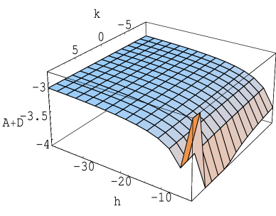
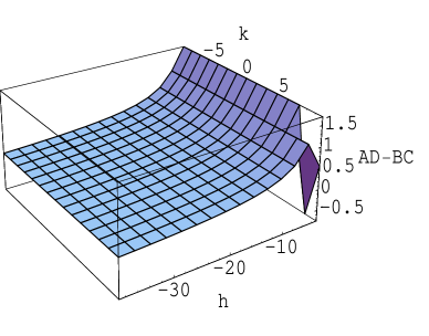
Figure 20: Only for negative eigenvalues, satisfying the conditions $A+D<0$ and $AD-BC>0$ the linear perturbations become small and the system may be stable.

Let us consider the following (homogeneous) perturbation around the critical solution (A.9) or (A.10):

$$x=x_{0}+\delta x,\qquad u=u_{0}+\delta u.$$ (A.20)

Since the functional form of the potential is already specified, the variation of $y$ is encoded into the variation of $\varphi$. For stability of the solution, under a small perturbation about the critical or fixed point solution, requires

$$A+D<0,\qquad AD-BC>0,$$ (A.21)

where $A,B,C,D$ are the eigenvalues of a $2\times 2$ matric, as given by

$$\frac{d}{dN}\left(\begin{array}[]{c}\delta x\\ \delta z\end{array}\right)=M\left(\begin{array}[]{c}\delta x\\ \delta z\end{array}\right),\qquad M=\left(\begin{array}[]{c}A\qquad B\\ C\qquad D\end{array}\right).$$ (A.22)

In the following, we define $V_{1}t_{1}^{2}\equiv k$. We find

$$A=-\frac{\tilde{A}}{hE},\quad B=-\frac{\tilde{B}}{\gamma E},\quad C=-\frac{\gamma\,\tilde{C}}{3h^{2}(3h^{2}-3h-2k)E},\quad D=-\frac{\tilde{D}}{hE}$$ (A.23)

where

$$\tilde{A} \equiv 18h^{4}(h-1)(9h^{2}-4h+1)+3k(1-24h)h^{2}+k^{2}(132h^{3}-22h^{2}-7h+1),$$

$$\tilde{B} \equiv 3(3h^{2}-3h-2k)\left(6h^{2}(3h^{2}-2h+1)-k(22h^{2}-13h+1)\right),$$ (A.25)

$$\tilde{C} \equiv \left(36h^{5}(3h^{2}-1)-2kh^{2}(72h^{3}+42h^{2}-12h(3h+2)+6)+2k^{2}(28h^{2}-12h+1)\right)$$ (A.26)

$$\times\,(9h^{3}-3h^{2}-6hk+k),$$

$$\tilde{D} = 36h^{4}(3h-1)(h-1)^{2}+2k^{2}(24h^{3}-68h^{2}+17h-1)-4kh^{2}(36h^{3}-93h^{2}+51h-6).$$

$${E} = 18h^{4}(5h^{2}-4h+1)+k^{2}(60h^{2}-16h+1)-6kh^{2}(25h^{2}+17h-2).$$ (A.28)

We find the result in [8] by taking $k=0$ . In the case $\gamma>0$ and $h<0$, all eigenvalues are negative, except when $|h|$ is small, $|h|\lesssim 2$, or when the parameter $k$ takes a large value (cf figure 20). While, for $\gamma<0$, two of them ($B$ and $C$) take positive values, leading to a classical instability of the critical solution. Such a system is normally unstable also under inhomogeneous (cosmological) perturbations. In particular, for a large and positive potential, so that $k\gg 0$, only the $h>0$ solution can be stable.

A.4 Fixed dilaton/modulus

It is quite plausible that after inflation the field $\varphi$ would remain almost frozen for a long time, so $x\simeq 0$, leading to an universe filled dominantly with radiation and highly relativistic or stiff matter. Such a phase of the universe is described by the solution

$$\Omega_{m}^{w=1}=\frac{1}{1+\Omega_{1}},\quad\Omega_{r}=\frac{\rho_{1}\,e^{2N}}{1+\Omega_{1}},\quad\epsilon=\frac{-3-2\rho_{1}\,e^{2N}}{1+\Omega_{1}},\quad y=\frac{3\rho_{2}\,e^{6N}}{1+\Omega_{1}}$$ (A.29)

where $\Omega_{1}\equiv\rho_{1}\,e^{2N}+\rho_{2}\,e^{6N}$ and $\rho_{i}$ are integration constants. One takes $\rho_{i}>0$, so that $\Omega_{r}>0$ and $V(\phi)\approx\Lambda$. The density fraction for a stiff fluid, $\Omega_{m}^{w=1}$, decreases quickly as the universe further expands, $N\gg 0$, thereby creating a vast amount of thermal radiation.

While, at late-times, $\varphi$ is again rolling slowly, such that $x\approx 0$. The cosmic expansion is then characterized by

$$\Omega_{m}^{w=0}=\frac{1}{1+\Omega_{2}},\quad\Omega_{r}=\frac{\delta_{1}e^{-N}}{1+\Omega_{2}},\quad\epsilon=\frac{-3-4\delta_{1}\,e^{-N}}{2+2\Omega_{2}},\quad y=\frac{3\delta_{1}\,e^{3N}}{1+\Omega_{2}}$$ (A.30)

where $\Omega_{2}\equiv\delta_{1}\,e^{-N}+\delta_{2}\,e^{3N}$ and $\delta_{i}$ are integration constants. Both $\Omega_{m}$ and $\Omega_{r}$ decrease with the expansion of the universe, but unlike a universe dominated by highly relativistic fluids or stiff-matter, the radiation energy density decreases now faster as compared to the matter energy density, as it is red-shifted away by a factor of $e^{-N}$.

References

- [1] A. G. Riess et al [Supernova Search Team Collaboration], Type Ia Supernova Discoveries at From the Hubble Space Telescope: Evidence for Past Deceleration and Constraints on Dark Energy Evolution, Astrophys. J. 607, 665 (2004).
- [2] D. N. Spergel et al [WMAP Collaboration], First Year Wilkinson Microwave Anisotropy Probe (WMAP) Observations: Determination of Cosmological Parameters, Astrophys. J. Suppl. 148, 175 (2003).
-
[3]
T. Padmanabhan,
Cosmological constant: The weight of the vacuum,
Phys. Rept. 380, 235 (2003)
[arXiv:hep-th/0212290];
E. J. Copeland, M. Sami and S. Tsujikawa, Dynamics of dark energy, Int. J. Mod. Phys. D 15 (2006) 1753 [arXiv:hep-th/0603057];
V. Sahni and A. Starobinsky, Reconstructing dark energy, arXiv:astro-ph/0610026. -
[4]
C. Wetterich,
Cosmology and the fate of dilatation symmetry,
Nucl. Phys. B 302, 668 (1988);
P. G. Ferreira and M. Joyce, Structure formation with a self-tuning scalar field, Phys. Rev. Lett. 79, 4740 (1997) [arXiv:astro-ph/9707286];
I. Zlatev, L. M. Wang and P. J. Steinhardt, Quintessence, Cosmic Coincidence, and the Cosmological Constant, Phys. Rev. Lett. 82, 896 (1999) [arXiv:astro-ph/9807002]. - [5] L. Amendola, Coupled quintessence, Phys. Rev. D 62, 043511 (2000) [arXiv:astro-ph/9908023].
-
[6]
C. Armendariz-Picon, T. Damour and V. F. Mukhanov, k-inflation, Phys. Lett. B 458, 209 (1999)
[arXiv:hep-th/9904075];
F. Piazza and S. Tsujikawa, Dilatonic ghost condensate as dark energy, JCAP 0407, 004 (2004) [arXiv:hep-th/0405054]. -
[7]
B. Boisseau, G. Esposito-Farese, D. Polarski and A. A. Starobinsky,
Reconstruction of a scalar-tensor theory of gravity in an accelerating
universe,
Phys. Rev. Lett. 85, 2236 (2000)
[arXiv:gr-qc/0001066];
E. Elizalde, S. Nojiri and S. D. Odintsov, Late time cosmology in (phantom) scalar-tensor theory: Dark energy and the cosmic speed-up, Phys. Rev. D 70, 043539 (2004) [arXiv:hep-th/0405034].
R. Gannouji, D. Polarski, A. Ranquet and A. A. Starobinsky, Scalar-tensor models of normal and phantom dark energy, astro-ph/0606287. - [8] S. Nojiri, S. D. Odintsov and M. Sasaki, Gauss-Bonnet dark energy, Phys. Rev. D 71, 123509 (2005) [arXiv:hep-th/0504052].
-
[9]
M. Sami, A. Toporensky, P. V. Tretjakov and S. Tsujikawa,
The fate of (phantom) dark energy universe with string curvature
corrections,
Phys. Lett. B 619, 193 (2005)
[arXiv:hep-th/0504154];
G. Calcagni, S. Tsujikawa and M. Sami, Dark energy and cosmological solutions in second-order string gravity, Class. Quant. Grav. 22, 3977 (2005) [arXiv:hep-th/0505193]. -
[10]
I. P. Neupane and B. M. N. Carter, Dynamical Relaxation of
Dark Energy: A Solution to Early Inflation,
Late time Acceleration and the Cosmological Constant Problem,
Phys. Lett. B 638, 94 (2006) [arXiv:hep-th/0510109];
I. P. Neupane and B. M. N. Carter, Towards inflation and dark energy cosmologies from modified Gauss-Bonnet theory, JCAP 0606, 004 (2006) [arXiv:hep-th/0512262]. -
[11]
I. P. Neupane,
On compatibility of string effective action with an accelerating
universe,
Class. Quant. Grav. 23, 7493 (2006)
[arXiv:hep-th/0602097];
I. P. Neupane, Towards inflation and accelerating cosmologies in string-generated gravity models, arXiv:hep-th/0605265. -
[12]
P. Creminelli, M. A. Luty, A. Nicolis and L. Senatore,
Starting the universe: Stable violation of the null energy condition and
non-standard cosmologies,
arXiv:hep-th/0606090;
N. Arkani-Hamed, H. C. Cheng, M. A. Luty and S. Mukohyama, Ghost condensation and a consistent infrared modification of gravity, JHEP 0405, 074 (2004) [arXiv:hep-th/0312099]. - [13] I. Y. Aref’eva and I. V. Volovich, On the null energy condition and cosmology, hep-th/0612098.
-
[14]
S. Capozziello, S. Carloni and A. Troisi,
Quintessence without scalar fields, astro-ph/0303041;
S. M. Carroll, V. Duvvuri, M. Trodden and M. S. Turner, Phys. Rev. D 70, 043528 (2004) [arXiv:astro-ph/0306438];
S. Nojiri and S. D. Odintsov, Modified gravity with ln R terms and cosmic acceleration, Gen. Rel. Grav. 36, 1765 (2004) [arXiv:hep-th/0308176]. - [15] I. Antoniadis, J. Rizos and K. Tamvakis, Singularity - free cosmological solutions of the superstring effective action, Nucl. Phys. B 415, 497 (1994) [arXiv:hep-th/9305025].
-
[16]
D. J. Gross and J. H. Sloan,
The quartic effective action for the heterotic string,
Nucl. Phys. B 291, 41 (1987);
I. Antoniadis, E. Gava and K. S. Narain, Moduli Corrections To Gauge And Gravitational Couplings In Four-Dimensional Superstrings, Nucl. Phys. B 383, 93 (1992) [arXiv:hep-th/9204030]. -
[17]
R. Easther and K. i. Maeda,
One-Loop Superstring Cosmology and the Non-Singular Universe,
Phys. Rev. D 54, 7252 (1996)
[arXiv:hep-th/9605173];
P. Kanti, J. Rizos and K. Tamvakis, Singularity-free cosmological solutions in quadratic gravity, Phys. Rev. D 59, 083512 (1999) [arXiv:gr-qc/9806085];
S. Kawai, M. a. Sakagami and J. Soda, Instability of 1-loop superstring cosmology, Phys. Lett. B 437, 284 (1998) [arXiv:gr-qc/9802033];
S. Tsujikawa, R. Brandenberger and F. Finelli, On the construction of nonsingular pre-big-bang and ekpyrotic cosmologies and the resulting density perturbations, Phys. Rev. D 66, 083513 (2002) [arXiv:hep-th/0207228]. - [18] P.J. Steinhardt and N.Turok, A cyclic model of the Universe, Science 296 (2002) 1436-39.
- [19] S. Tsujikawa and M. Sami, String-inspired cosmology: Late time transition from scaling matter era to dark energy universe caused by a Gauss-Bonnet coupling, JCAP 0701 (2007) 006 [arXiv:hep-th/0608178].
-
[20]
T. Koivisto and D. F. Mota,
Cosmology and Astrophysical Constraints of Gauss-Bonnet Dark Energy,
Phys. Lett. B 644 (2007) 104 [arXiv:astro-ph/0606078]
T. Koivisto and D. F. Mota, Gauss-Bonnet quintessence: Background evolution, large scale structure and cosmological constraints, Phys. Rev. D 66, 023518 (2007) [arXiv:hep-th/0609155]. - [21] A. Coc, K. A. Olive, J. P. Uzan and E. Vangioni, Big bang nucleosynthesis constraints on scalar-tensor theories of gravity, Phys. Rev. D 73, 083525 (2006) [arXiv:astro-ph/0601299].
- [22] T. Damour, F. Piazza and G. Veneziano, Violations of the equivalence principle in a dilaton-runaway scenario, Phys. Rev. D 66, 046007 (2002) [arXiv:hep-th/0205111].
- [23] T. Damour, G. W. Gibbons and C. Gundlach, Dark Matter, Time Varying G, And A Dilaton Field, Phys. Rev. Lett. 64, 123 (1990).
- [24] J. Martin, C. Schimd and J. P. Uzan, Testing for in the solar system, Phys. Rev. Lett. 96, 061303 (2006) [arXiv:astro-ph/0510208].
- [25] J. Khoury and A. Weltman, Chameleon fields: Awaiting surprises for tests of gravity in space, Phys. Rev. Lett. 93, 171104 (2004) [arXiv:astro-ph/0309300].
- [26] D. F. Mota and D. J. Shaw, Evading equivalence principle violations, astrophysical and cosmological constraints in scalar field theories with a strong coupling to matter, Phys. Rev. D 75, 063501 (2007) [arXiv:hep-ph/0608078].
- [27] L. Amendola, C. Charmousis and S. C. Davis, Constraints on Gauss-Bonner gravity in dark energy cosmologies, JCAP 0612 (2006) 020 [arXiv:hep-th/0506137].
- [28] G. Calcagni, B. de Carlos and A. De Felice, Ghost conditions for Gauss-Bonnet cosmologies, Nucl. Phys. B 752, 404 (2006) [arXiv:hep-th/0604201].
-
[29]
J. c. Hwang and H. Noh,
Cosmological perturbations in generalized gravity theories,
Phys. Rev. D 54, 1460 (1996);
C. Cartier, J. c. Hwang and E. J. Copeland, Evolution of cosmological perturbations in non-singular string cosmologies, Phys. Rev. D 64, 103504 (2001) [arXiv:astro-ph/0106197];
J. c. Hwang and H. Noh, Classical evolution and quantum generation in generalized gravity theories including string corrections and tachyon: Unified analyses, Phys. Rev. D 71, 063536 (2005) [arXiv:gr-qc/0412126]. -
[30]
I. P. Neupane,
Accelerating cosmologies from exponential potentials,
Class. Quant. Grav. 21, 4383 (2004)
[arXiv:hep-th/0311071];
I. P. Neupane, Cosmic acceleration and M theory cosmology, Mod. Phys. Lett. A 19, 1093 (2004) [arXiv:hep-th/0402021];
I. P. Neupane and D. L. Wiltshire, Cosmic acceleration from M theory on twisted spaces, Phys. Rev. D 72, 083509 (2005) [arXiv:hep-th/0504135]; I.P. Neupane, hep-th/0609086. -
[31]
S. Nojiri, S. D. Odintsov and M. Sami,
Dark energy cosmology from higher-order, string-inspired
gravity and its reconstruction,
arXiv:hep-th/0605039.
G. Cognola, E. Elizalde, S. Nojiri, S. Odintsov and S. Zerbini, String-inspired Gauss-Bonnet gravity reconstructed from the universe expansion history and yielding the transition from matter dominance to dark energy, arXiv:hep-th/0611198. - [32] Z. K. Guo, N. Ohta and S. Tsujikawa, Realizing scale-invariant density perturbations in low-energy effective string theory, Phys. Rev. D 75 (2007) 023520 [arXiv:hep-th/0610336].
-
[33]
E. D. Stewart and D. H. Lyth,
A More accurate analytic calculation of the spectrum of cosmological
perturbations produced during inflation,
Phys. Lett. B 302, 171 (1993)
[arXiv:gr-qc/9302019];
E. J. Copeland, E. W. Kolb, A. R. Liddle and J. E. Lidsey, Reconstructing the inflaton potential: Perturbative reconstruction to second order, Phys. Rev. D 49, 1840 (1994) [arXiv:astro-ph/9308044]. - [34] H. Peiris and R. Easther, Recovering the Inflationary Potential and Primordial Power Spectrum With a Slow Roll Prior: Methodology and Application to WMAP 3 Year Data, JCAP 0607, 002 (2006) [arXiv:astro-ph/0603587].
- [35] S. Kanno and J. Soda, Lorentz violating inflation, Phys. Rev. D 74, 063505 (2006) [arXiv:hep-th/0604192].
-
[36]
G. Esposito-Farese and D. Polarski,
Scalar-tensor gravity in an accelerating universe,
Phys. Rev. D 63, 063504 (2001)
[arXiv:gr-qc/0009034];
G. Esposito-Farese, Tests of scalar-tensor gravity, AIP Conf. Proc. 736, 35 (2004) [arXiv:gr-qc/0409081];
T. P. Sotiriou and E. Barausse, Post-Newtonian expansion for Gauss-Bonnet gravity, arXiv:gr-qc/0612065. - [37] G. N. Felder, L. Kofman and A. D. Linde, Instant preheating, Phys. Rev. D 59, 123523 (1999) [arXiv:hep-ph/9812289].
- [38] A. De Felice, M. Hindmarsh and M. Trodden, Ghosts, instabilities, and superluminal propagation in modified gravity models, JCAP 0608, 005 (2006) [arXiv:astro-ph/0604154].
- [39] Y. Wang and M. Tegmark, New dark energy constraints from supernovae, microwave background and galaxy clustering, Phys. Rev. Lett. 92, 241302 (2004) [arXiv:astro-ph/0403292].
-
[40]
A. G. Riess et al.,
New Hubble Space Telescope Discoveries of Type Ia Supernovae at :
Narrowing Constraints on the Early Behavior of Dark Energy,
arXiv:astro-ph/0611572;
P. Astier et al., The Supernova Legacy Survey: Measurement of , and from the First Year Data Set, Astron. Astrophys. 447, 31 (2006) [arXiv:astro-ph/0510447]. - [41] U. Alam, V. Sahni and A. A. Starobinsky, Exploring the Properties of Dark Energy Using Type Ia Supernovae and Other Datasets, arXiv:astro-ph/0612381.
-
[42]
S. M. Carroll, M. Hoffman and M. Trodden,
Can the dark energy equation of state parameter w be less than ?,
Phys. Rev. D 68, 023509 (2003) [astro-ph/0301273];
P. Singh, M. Sami and N. Dadhich, Cosmological dynamics of phantom field, Phys. Rev. D 68, 023522 (2003) [arXiv:hep-th/0305110];
U. Alam, V. Sahni and A. A. Starobinsky, The case for dynamical dark energy revisited, JCAP 0406, 008 (2004) [arXiv:astro-ph/0403687];
W. Hu, Crossing the phantom divide: Dark energy internal degrees of freedom, Phys. Rev. D 71, 047301 (2005) [arXiv:astro-ph/0410680];
S. Nojiri, S. D. Odintsov and S. Tsujikawa, Properties of singularities in (phantom) dark energy universe, Phys. Rev. D 71, 063004 (2005) [arXiv:hep-th/0501025];
H. K. Jassal, J. S. Bagla and T. Padmanabhan, Observational constraints on low redshift evolution of dark energy: How consistent are different observations?, Phys. Rev. D 72, 103503 (2005) [arXiv:astro-ph/0506748];
L. Perivolaropoulos, Crossing the phantom divide barrier with scalar tensor theories, JCAP 0510, 001 (2005) [arXiv:astro-ph/0504582];
M. z. Li, B. Feng and X. m. Zhang, A single scalar field model of dark energy with equation of state crossing , JCAP 0512, 002 (2005) [arXiv:hep-ph/0503268];
I. Y. Aref’eva, A. S. Koshelev and S. Y. Vernov, Crossing of the barrier by D3-brane dark energy model, Phys. Rev. D 72, 064017 (2005) [arXiv:astro-ph/0507067];
P. S. Apostolopoulos and N. Tetradis, Late acceleration and w = -1 crossing in induced gravity, Phys. Rev. D 74, 064021 (2006) [arXiv:hep-th/0604014];
Z. G. Huang, H. Q. Lu and W. Fang, Dilaton coupled quintessence model in the omega-omega’ plane, arXiv:hep-th/0610018;
H. Wei and R. G. Cai, A note on crossing the phantom divide in hybrid dark energy model, Phys. Lett. B 634, 9 (2006) [arXiv:astro-ph/0512018];
H. Wei and R. G. Cai, Interacting vector-like dark energy, the first and second cosmological coincidence problems, Phys. Rev. D 73, 083002 (2006) [arXiv:astro-ph/0603052];
Z. G. Huang, H. Q. Lu and W. Fang, Coupled quintessence and phantom based on dilaton, Class. Quant. Grav. 23, 6215 (2006) [arXiv:hep-th/0604160]; - [43] C. Bonvin, C. Caprini and R. Durrer, A no-go theorem for k-essence dark energy, Phys. Rev. Lett. 97, 081303 (2006) [arXiv:astro-ph/0606584].
- [44] A. A. Starobinsky, Phys. Lett. B 91, 99 (1980).