Primordial perturbations from slow-roll inflation on a brane

Abstract

In this paper we quantise scalar perturbations in a Randall-Sundrum-type model of inflation where the inflaton field is confined to a single brane embedded in five-dimensional anti-de Sitter space-time. In the high energy regime, small-scale inflaton fluctuations are strongly coupled to metric perturbations in the bulk and gravitational back-reaction has a dramatic effect on the behaviour of inflaton perturbations on sub-horizon scales. This is in contrast to the standard four-dimensional result where gravitational back-reaction can be neglected on small scales. Nevertheless, this does not give rise to significant particle production, and the correction to the power spectrum of the curvature perturbations on super-horizon scales is shown to be suppressed by a slow-roll parameter. We calculate the complete first order slow-roll corrections to the spectrum of primordial curvature perturbations.

I Introduction

Recent developments have suggested that our four-dimensional Universe could lie on a brane embedded in a higher-dimensional space-time Review . This new perspective may dramatically change our picture of the early Universe. One of the most studied scenarios is the model proposed by Randall and Sundrum where a single brane is embedded in five-dimensional anti-de Sitter (adS) space-time RS99 . In this model, the Friedmann equation is modified at high energy densities BDEL and the bulk gravity is strongly coupled to the dynamics on the brane. Because of that inflation in the early Universe, and the perturbations generated during inflation, could be significantly modified compared with conventional four-dimensional models.

The simplest way to realize inflation in the brane world is to consider inflation driven by the potential energy of a scalar field, the inflaton, confined to the brane MWBH99 . The amplitude of the resulting scalar curvature perturbations is given by

$$\langle{\cal R}_{c}^{2}\rangle^{1/2}=\left(\frac{H}{\dot{\phi}}\right)\langle\delta\phi^{2}\rangle^{1/2},$$ (1)

where $H$ is the Hubble parameter, $\dot{\phi}$ is the time derivative of the inflaton $\phi$, and $\delta\phi$ is the inflaton fluctuation on a spatially flat hypersurface. The quantum expectation value of the inflaton fluctuations on super-horizon scales in the de Sitter space-time is

$$\langle\delta\phi^{2}\rangle=\left(\frac{H}{2\pi}\right)^{2}.$$ (2)

It has been shown that the constancy of the curvature perturbation ${\cal R}_{c}$ on comoving hypersurfaces outside the horizon is independent of the gravitational theory WMLL and thus it is also valid in this brane-world model LMSW . The curvature perturbation, Eq. (1), can thus be directly related to the observables like Cosmic Microwave Background (CMB) temperature anisotropy. Although the formula for the curvature perturbation is exactly the same as in the four-dimensional case, the relation between the Hubble parameter $H$ and the scalar field potential $V$ is modified at high energy densities due to the modification of the Friedmann equation MWBH99 . This changes the prediction of the spectrum of scalar perturbations for a given potential. Based on Eq. (1), interesting progress has been made on observational predictions of the brane-world inflation models obs ; RL .

A crucial assumption in deriving Eq. (2), and hence calculating the amplitude of the curvature perturbation (1), is that back-reaction due to metric perturbations in the bulk can be neglected. In the extreme slow-roll limit, where the coupling between inflaton fluctuations and metric perturbations vanishes, this assumption must be valid, but it is not obvious whether this assumption is still valid once slow-roll effects are taken into account. Ref. KLMW initiated the study of bulk metric perturbations generated by inflaton fluctuations on a brane. It was shown that sub-horizon inflaton fluctuations on a brane excite an infinite ladder of Kaluza–Klein modes of the bulk metric perturbations already at the first order in slow-roll parameters. Subsequently Ref. KMW found that, due to this infinite ladder of modes, a naive slow-roll expansion breaks down in the high energy regime once one takes into account the back-reaction of the bulk metric perturbations. This was confirmed in Ref. HK by direct numerical simulations that solved the coupled equations for inflaton perturbations and bulk metric perturbations without using any slow-roll approximation.

Although these results indicate that the back-reaction of the bulk metric perturbations give rise to corrections of order one to the behaviour of inflaton fluctuations on sub-horizon scales even in slow-roll inflation, this does not necessarily imply that the amplitude of the inflaton perturbations receives corrections of order one on large scales. In order to address the amplitude of the inflaton perturbations, and hence the curvature perturbations (1) on large scales, we need to quantise properly the coupled brane inflaton fluctuations and bulk metric perturbations. The purpose of this paper is to perform quantisation of the coupled fluctuations and determine the corrections to the inflaton fluctuations amplitude, Eq. (2). In this way we study whether the bulk metric perturbations give rise to a significant modification of the amplitude of the primordial fluctuations, Eq. (1), generated during high-energy inflation on a brane.

This paper is organised as follows. In section II, we begin by describing the model and present the coupled equations for the inflaton fluctuations on a brane and the metric perturbations in the bulk. Slow-roll parameters are defined and our approximation for dealing with the brane-bulk coupling is explained. Based on this approximation, late-time solutions are derived. In section III, we study the behaviour of the bound states, which determine the final amplitude of the curvature perturbations. We perform numerical simulations to evolve the late-time bound states backwards in time and to find their early-time behaviour. We also develop a semi-analytic method to derive solutions for the bound states at early times. The bound states are shown to consist of an infinite ladder of the Kaluza–Klein modes. Using the semi-analytic analysis, asymptotic solutions for perturbations on small scales are derived. Section IV is devoted to the quantisation of the bound states. We present a method to determine the quantum amplitude of fluctuations with the knowledge of asymptotic solutions for the bound states on small scales. Then the corrections to the formula (1) at the first order in the slow-roll parameters are presented and compared with the standard slow-roll corrections in four-dimensional gravity. We end up with our conclusions in Section V.

II Description of the Model

II.1 Basic equations

We take as a starting point the analyses of Refs. KLMW ; KMW ; HK . The model under consideration is the single-brane Randall–Sundrum model RS99 with a cosmological constant in the bulk and an inflaton field $\phi$ confined to the brane, whose potential $V(\phi)$ satsifies the slow-roll conditions. The action for the model is

$$S=\frac{1}{2\kappa_{5}^{2}}\int_{\cal M}d^{5}x\sqrt{-^{{}^{(5)}}\!g}\>\Big{\{}R-2\Lambda\Big{\}}+\int_{\partial\cal M}d^{4}x\sqrt{-^{{}^{(4)}}\!g}\left\{-\lambda+\frac{1}{\kappa_{5}^{2}}K\right\}-\int d^{4}x\sqrt{-^{{}^{(4)}}\!g}\left\{\frac{1}{2}(\partial\phi)^{2}+V(\phi)\right\},$$ (3)

where $K$ is the trace of the extrinsic curvature of the boundary ${\partial\cal M}$ and $\lambda$ is the tension. The adS curvature scale is defined by $\Lambda=-6\mu^{2}$ and the tension is tuned as $\lambda=6\mu/\kappa_{5}^{2}$.

The background line element has the form

$$ds^{2}=-N^{2}(y,t)dt^{2}+A^{2}(y,t)\delta_{ij}dx^{i}dx^{j}+dy^{2}.$$ (4)

Here the warp function $A(y,t)$ and the lapse function $N(y,t)$ are BDEL

$$A(y,t) =a(t)\left\{\cosh(\mu y)-\left(1+\frac{\kappa_{5}^{2}\rho}{6\mu}\right)\sinh(\mu y)\right\},$$ (5)

$$N(y,t) =\cosh(\mu y)-\left\{1-\frac{\kappa_{5}^{2}}{6\mu}(2\rho+3p)\right\}\sinh(\mu y),$$ (6)

where

$$\rho=\frac{1}{2}\dot{\phi}^{2}+V(\phi),\quad p=\frac{1}{2}\dot{\phi}^{2}-V(\phi).$$ (7)

In these coordinates, the brane is located at $y=y_{\rm b}=0$. The scale factor is determined by the Friedmann equation and the equation of motion for the scalar field,

$$H^{2} = \frac{\kappa_{4}^{2}}{3}\rho\left(1+\frac{\rho}{2\lambda}\right),\quad\ddot{\phi}+3H\dot{\phi}+V^{\prime}(\phi)=0.$$ (8)

Allowing for the linearised metric perturbations gives the metric

$$ds^{2}=-N(y,t)^{2}(1+2{\cal A})dt^{2}+A(y,t)^{2}(1+2{\cal R})\delta_{ij}dx^{i}dx^{j}\\ +(1+2A_{yy})dy^{2}+N(y,t)A_{y}dydt.$$ (9)

It was shown in Refs Mukohyama ; Kodama that the perturbed five-dimensional Einstein equations are solved in the adS background if the metric perturbations are derived from a master variable $\Omega$:

$${\cal A} =-\frac{1}{6A}\left\{\left(2\Omega^{\prime\prime}-\frac{N^{\prime}}{N}\Omega^{\prime}\right)+\frac{1}{N^{2}}\left(\ddot{\Omega}-\frac{\dot{N}}{N}\dot{\Omega}\right)-\mu^{2}\Omega\right\}\,,$$ (10)

$$A_{y} =\frac{1}{NA}\left(\dot{\Omega}^{\prime}-\frac{N^{\prime}}{N}\dot{\Omega}\right)\,,$$ (11)

$$A_{yy} =\frac{1}{6A}\left\{\left(\Omega^{\prime\prime}-2\frac{N^{\prime}}{N}\Omega^{\prime}\right)+\frac{2}{N^{2}}\left(\ddot{\Omega}-\frac{\dot{N}}{N}\dot{\Omega}\right)+\mu^{2}\Omega\right\}\,,$$ (12)

$${\cal R} =\frac{1}{6A}\left\{\left(\Omega^{\prime\prime}+\frac{N^{\prime}}{N}\Omega^{\prime}\right)+\frac{1}{N^{2}}\left(-\ddot{\Omega}+\frac{\dot{N}}{N}\dot{\Omega}\right)-2\mu^{2}\Omega\right\}\,.$$ (13)

The remaining perturbed five-dimensional Einstein equation then gives the wave equation in the bulk,

$$-\left(\frac{1}{NA^{3}}\dot{\Omega}\right)^{\cdot}+\left(\frac{N}{A^{3}}\Omega^{\prime}\right)^{\prime}+\left(\mu^{2}-\frac{k^{2}}{A^{2}}\right)\frac{N}{A^{3}}\Omega=0\,,$$ (14)

for perturbations with comoving wavenumber $k$ on the brane.

On the brane, there is also the perturbation of the inflaton $\delta\phi$. It is useful to express the scalar field perturbations $\delta\phi$ on the brane in terms of the gauge invariant, Mukhanov–Sasaki variable Mukhanov

$$Q\equiv\delta\phi-\frac{\dot{\phi}}{H}{\cal R}_{\rm b},$$ (15)

where subscript b denotes the quantity evaluated at the brane. The equation of motion is HK

$$\ddot{Q}+3H\dot{Q}+\frac{k^{2}}{a^{2}}Q+\left\{\frac{\ddot{H}}{H}-2\frac{\dot{H}}{H}\frac{V^{\prime}(\phi)}{\dot{\phi}}-2\left(\frac{\dot{H}}{H}\right)^{2}+V^{\prime\prime}(\phi)\right\}Q=J(\Omega),$$ (16)

where

$$J(\Omega)=-\frac{\dot{\phi}}{H}\left[\left(-\frac{\dot{H}}{H}+\frac{\ddot{H}}{2\dot{H}}\right)\kappa_{4}^{2}\delta q_{{\cal E}}+\frac{1}{3}\left(1-\frac{\dot{H}}{2{\cal H}^{2}}\right)\kappa_{4}^{2}\delta\rho_{{\cal E}}+\frac{1}{3}\kappa_{4}^{2}k^{2}\delta\pi_{{\cal E}}+\frac{1}{3}\frac{\dot{H}}{{\cal H}^{2}}\frac{k^{2}}{a^{2}}{\cal R}_{\rm b}\right],$$ (17)

${\cal H}=(A^{\prime}/A)_{\rm b}$ and $\kappa_{4}^{2}=\kappa_{5}^{2}\mu$. Here

$$\kappa_{4}^{2}\delta\rho_{\cal E} =\left(\frac{k^{4}\Omega}{3a^{5}}\right)_{\rm b},$$ (18)

$$\kappa_{4}^{2}\delta q_{{\cal E}} =-\frac{k^{2}}{3a^{3}}\left(H\Omega-\dot{\Omega}\right)_{\rm b},$$ (19)

$$\kappa_{4}^{2}\delta\pi_{{\cal E}} =\frac{1}{6a^{3}}\left\{3\ddot{\Omega}-3H\dot{\Omega}+\frac{k^{2}}{a^{2}}\Omega-3\left(\frac{N^{\prime}}{N}-\frac{A^{\prime}}{A}\right)\Omega^{\prime}\right\}_{\rm b}$$ (20)

come form the projected Weyl tensor SMS ; Deffayet , while the curvature perturbation, Eq. (13), evaluated at the brane is given in terms of $\Omega$ as

$${\cal R}_{\rm b}=\frac{1}{6a}\left(3{\cal H}\Omega^{\prime}-3H\dot{\Omega}-3\mu^{2}\Omega+\frac{k^{2}}{a^{2}}\Omega\right)_{\rm b}.$$ (21)

The junction condition, which describes how the brane field provides the boundary condition for the bulk metric perturbation is HK

$$\kappa_{5}^{2}a\dot{\phi}^{2}\left(\frac{H}{\dot{\phi}}Q\right)^{\cdot}=-\frac{k^{2}}{a^{2}}\left\{\frac{\kappa_{5}^{2}\dot{\phi}^{2}}{6}\left(\dot{\Omega}-H\Omega\right)+H\left(\Omega^{\prime}-\frac{A^{\prime}}{A}\Omega\right)\right\}_{\rm b}.$$ (22)

The master equation (14), the Mukhanov–Sasaki equation (16) with a source (17) and the junction condition (22) describe the coupled system of the inflaton and metric perturbations.

II.2 Slow-roll inflation

The slow-roll parameters are defined as

$$\epsilon_{{}_{H}}=-\frac{\dot{H}}{H^{2}},\quad\eta_{{}_{H}}=-\frac{\ddot{\phi}}{H\dot{\phi}}\;.$$ (23)

In terms of the scalar potential, these parameters are given by MWBH99

$$\epsilon_{{}_{H}} = \frac{1}{2\kappa_{4}^{2}}\left(\frac{V^{\prime}}{V}\right)^{2}\left[\frac{2\lambda(2\lambda+2V)}{(2\lambda+V)^{2}}\right],$$ (24)

$$\eta_{{}_{H}} = \frac{1}{\kappa_{4}^{2}}\left(\frac{V^{\prime\prime}}{V}\right)\left(\frac{2\lambda}{2\lambda+V}\right)-\epsilon_{{}_{H}}\;.$$ (25)

Self-consistency of the slow-roll approximation requires $\epsilon_{{}_{H}},|\eta_{{}_{H}}|\ll 1$. In the high energy regime, $V\gg\lambda$ (equivalently $H/\mu\gg 1$), the modification of the Friedmann equation eases the condition for slow-roll inflation for a given potential.

The amplitude of the scalar perturbations is determined by the curvature perturbations on a comoving hypersurface, which is conserved on large scales:

$${\cal R}_{c}=-\frac{H}{\dot{\phi}}Q.$$ (26)

At the zeroth order in the slow-roll parameters, the quantum expectation value of squared $Q$ is $\langle Q^{2}\rangle=(H/2\pi)^{2}$. Slow-roll dynamics of the inflaton field gives corrections to this result. One contribution comes from the evolution of $Q$ on super-horizon scales. As is seen from Eq. (16), deviations from the de Sitter space-time give an effective mass to $Q$ and modify the behaviour of $Q$ outside the horizon. In four-dimensional cosmology this correction is known as the Stewart–Lyth correction. This Stewart–Lyth correction in the present brane-world inflation model was calculated in Ref. RL assuming that the coupling to the bulk metric perturbations could be neglected.

In four-dimensional cosmology, the slow-roll corrections do not affect the dynamics of $Q$ on sub-horizon scales, as the effective mass induced by the dynamics of the inflaton can be neglected in comparison with the gradient term. It is then possible to quantise $Q$ as an effectively massless field in the de Sitter space-time. However, in the brane-world case there is no reason to believe that the coupling to the bulk metric perturbations can be neglected on sub-horizon scales. In fact in Refs. KMW ; HK it is shown that the coupling to the bulk metric perturbations can lead to $O(1)$ effect on the behaviour of $Q$ on small scales at high energies ($H/\mu\gg 1$) even though the coupling is suppressed by the slow-roll parameter. However, it has been an open question how this coupling affects the quantum amplitude of $Q$ on larger scales. The aim of this paper is to investigate the effect which the mixing between the bulk metric perturbations and the brane inflaton fluctuations has on the quantum amplitude of $Q$ after crossing out the horizon. We are only interested in corrections of the first order in the slow-roll parameters. Thus, we can study separately the effect of the brane-bulk coupling and other slow-roll corrections. Almost to the end of this paper we neglect all the slow-roll corrections in the equations of motion except for the coupling between $Q$ and $\Omega$, as we study the effect of the brane-bulk coupling.

II.3 de Sitter approximation

As explained above, we assume zeroth-order slow-roll for the background everywhere except for the terms inducing the mixing between the bulk and brane perturbations. This means that, in practice, we consider the background as the de Sitter brane configuration Kaloper ,

$${\rm d}s^{2}=N(z)^{2}\left[{\rm d}z^{2}+\frac{1}{H^{2}\tau^{2}}\big{(}-{\rm d}\tau^{2}+\delta_{ij}dx^{i}dx^{j}\big{)}\right]\,,$$ (27)

where

$$N(z)=\frac{H}{\mu\sinh(Hz)}\,,$$ (28)

and the brane is located at

$$z_{\rm b}=H^{-1}{\,\text{arcsinh}}\left(\frac{H}{\mu}\right)\,.$$ (29)

Here, $H$ is the Hubble parameter (constant in the de Sitter Universe) and $\tau$ is the conformal time coordinate. Hereafter we redefine the time variable

$$\tau\to-\tau\,,$$ (30)

so that evolution forward in $\tau$ is evolution backwards in time.

It is convenient to define a new variable $\chi$, related to the master variable as follows,

$$\Omega=k^{-2}a^{2}N^{3/2}\chi\,.$$ (31)

The equation of motion for $\chi$ derived from Eq. (14) is

$$\chi_{,\tau\tau}+k^{2}\chi-\frac{2}{\tau^{2}}\chi+\frac{1}{H^{2}\tau^{2}}\big{(}-\chi^{\prime\prime}+U(z)\chi\big{)}=0\,,$$ (32)

where

$$U(z)=\frac{H^{2}}{4}\left(9-\frac{1}{\sinh^{2}(Hz)}\right)\,.$$ (33)

Note that Eq. (32) is separable. The other equations are simplified by defining a new brane variable

$$u=aQ+\frac{\dot{\phi}}{6H}\chi|_{{}_{\rm b}}\,.$$ (34)

It obeys the following equation of motion,

$$u_{,\tau\tau}+k^{2}u-\frac{2}{\tau^{2}}u=\frac{\dot{\phi}}{3H\tau}\left[\chi_{,\tau}-\frac{2}{\tau}\chi\right]_{{}_{\rm b}}\,,$$ (35)

derived from Eq. (16), and the junction condition

$$\left[\chi^{\prime}+\left(\frac{1}{2}\frac{N^{\prime}}{N}+\frac{\kappa_{5}^{2}\dot{\phi}^{2}}{3}\right)\chi\right]_{{}_{\rm b}}=\kappa_{5}^{2}\dot{\phi}H\left[\tau u_{,\tau}-u\right],$$ (36)

derived from Eq. (22). Here we have neglected all terms suppressed by the slow-roll parameters except for the terms responsible for the coupling between $u$ and $\chi$, i.e., the terms that induce the mixing between the brane and bulk modes. The latter terms at the first non-trivial order in slow-roll are $O(\beta)$, where

$$\beta^{2}=\frac{\kappa_{5}^{2}\dot{\phi}^{2}}{6H}.$$ (37)

To the leading order in the slow-roll parameters, $\beta^{2}$ can be written as

$$\beta^{2}=\frac{1}{3}\epsilon_{{}_{H}}\left(1+\left(\frac{\mu}{H}\right)^{2}\right)^{-1/2}\;.$$ (38)

This is the parameter that controls the strength of the coupling between the inflaton perturbation on the brane and the gravitational perturbations in the bulk.

The second order action for the variables $\Omega$ and $Q$ has been derived in Ref. YK . In terms of $u$ and $\chi$, the action is

$$S = \int d^{4}x\left[\frac{1}{2}(u_{,\tau}^{2}-k^{2}u^{2}+\frac{2}{\tau^{2}}u^{2})+\frac{\dot{\phi}}{3H}\left(\frac{u\chi_{,\tau}}{\tau}-\frac{2u\chi}{\tau^{2}}\right)\right]$$ (39)

$$+ \frac{1}{6\kappa_{5}^{2}}\int d^{4}xdz\left[\chi_{,\tau}^{2}-k^{2}\chi^{2}+\frac{2}{\tau^{2}}\chi^{2}-\frac{{\chi^{\prime}}^{2}+U(z)\chi^{2}}{(H\tau)^{2}}\right]+\frac{1}{6\kappa_{5}^{2}}\left[\frac{1}{2}\left(\frac{N^{\prime}}{N}\right)_{{}_{\rm b}}+\frac{\kappa_{5}^{2}\dot{\phi}^{2}}{3}\right]\int d^{4}x\frac{1}{(H\tau)^{2}}\chi^{2}\,.$$

From this action, the coupled equations (32), (35) and (36) can be derived. It is useful to define the time-independent Wronskian of two solutions,

$$W(f^{*},f)=u^{*}u_{,\tau}-uu_{,\tau}^{*}-\frac{\dot{\phi}}{3H\tau}\big{(}u^{*}\chi|_{{}_{\rm b}}-u\chi^{*}|_{{}_{\rm b}}\big{)}+\frac{1}{3\kappa_{5}^{2}}\int^{\infty}_{z_{{}_{\rm b}}}dz\,\big{(}\chi^{*}\chi_{,\tau}-\chi\chi_{,\tau}^{*}\big{)}\,,$$ (40)

where $f=(u,\chi)$ is a state comprising a brane and a bulk mode. The Wronskian will play an important role in quantisation.

Without mixing, $u$ and $\chi$ would behave as canonical scalar fields in four dimensions and five dimensions, respectively. The existence of the mixing terms in the field equations and in the Wronskian makes the analysis complicated. We simplify the equations further by defining yet another new variable to describe the perturbations of the inflaton field on the brane,

$$\xi=u_{,\tau}+\frac{1}{\tau}u-\frac{\dot{\phi}}{3H}\frac{1}{\tau}\chi|_{{}_{\rm b}}\,,$$ (41)

which is related to the density perturbation on a comoving hypersurface Kodama . The brane equation of motion (35) is now written as

$$\xi_{,\tau\tau}+k^{2}\xi=-\frac{k^{2}\dot{\phi}}{3H\tau}\chi|_{{}_{\rm b}}\,,$$ (42)

and the junction condition (36) becomes

$$\left[\chi^{\prime}+\frac{1}{2}\frac{N^{\prime}}{N}\chi\right]_{{}_{\rm b}}=\kappa_{5}^{2}\dot{\phi}H\tau\xi\,.$$ (43)

Upon substituting (41) into (40), the Wronskian becomes

$$W(f^{*},f)=\frac{1}{k^{2}}(\xi^{*}\xi_{,\tau}-\xi\xi_{,\tau}^{*})+\frac{1}{3\kappa_{5}^{2}}\int^{\infty}_{z_{{}_{\rm b}}}dz\,\big{(}\chi^{*}\chi_{,\tau}-\chi\chi_{,\tau}^{*}\big{)}\,,$$ (44)

where $f=(\xi,\chi)$.

In this and next sections we are going to study the coupled system of equations (32), (35) and (36), or, equivalently, (32), (42) and (43).

II.4 Late time solutions

At late times, it is possible to find analytic solutions to the coupled equations. Solutions divide into bound states and continuum modes. There are two independent bound state solutions KLMW . A growing bound state solution is

$$u_{g}=\frac{A_{g}}{\tau}+B\tau\,,\quad\chi_{g}=C_{g}\,\tau\sqrt{\sinh(Hz)}\,\log\left(\frac{\cosh(Hz)-1}{\cosh(Hz)+1}\right)\,,$$ (45)

where $A_{g}$ is the overall amplitude, while $B$ and $C_{g}$ can be determined through $A_{g}$. In terms of $\xi$, the growing mode solution is given by

$$\xi_{g}=k^{2}A_{g},$$ (46)

which is clearly the growing mode solution of Eq. (42) at late times $k\tau\to 0$. A decaying bound state is given by

$$u_{d}=A_{d}\tau^{2}\,,\quad\chi_{d}=C_{d}\,\tau^{2}\sqrt{\sinh(Hz)}\left[1+\frac{\cosh(Hz)}{2}\log\left(\frac{\cosh(Hz)-1}{\cosh(Hz)+1}\right)\right]\,,$$ (47)

where $C_{d}$ is linearly related to $A_{d}$. We will re-derive these solutions later on in a slightly different language. For the time being we do not need explicit relations between the coefficients entering (45) or (47).

On the other hand, the continuum modes are

$$u_{\lambda}=g_{\lambda}\tau^{\alpha_{\lambda}},\quad\chi_{\lambda}=f_{\lambda}(z)\tau^{\alpha_{\lambda}},$$ (48)

where

$$\alpha_{\lambda}=\frac{1}{2}\pm i\lambda\,,$$ (49)

and in the high energy regime

$$f_{\lambda}(z)=N_{\lambda}\cos(\lambda z+\beta_{\lambda}).$$ (50)

The coupled equations determine $g_{\lambda}$ and $\beta_{\lambda}$ in terms of $N_{\lambda}$. Again, we do not need the explicit relations here and in what follows. It suffices to say that using these solutions, one can check that the Wronskian between the bound states and the continuum modes vanishes as $\tau\to 0$, and hence at all $\tau$. In other words, they are orthogonal to each other. Furthermore, unlike the growing bound state solution, the continuum modes decay away as $\tau\to 0$, so they do not have any effect at super-horizon scales. Thus, we focus on the bound states in the rest of this paper.

We are interested in the final amplitude of perturbations, which is determined by the the growing bound state. On large scales, the growing mode gives

$${\cal R}_{c}=-\frac{H^{2}}{\dot{\phi}}A_{g}\,.$$ (51)

The amplitude $A_{g}$ has to be determined by quantisation of the inflaton and metric fields on sub-horizon scales. We thus have to evolve the growing bound state backwards in time. For reasons that will become clear later, the early-time behaviour of the decaying bound state is also of importance.

III Bound-state solutions

III.1 Numerical analysis

We now investigate what becomes of the bound states at early times. By using the numerical method developed in Ref. HK , the coupled equations are evolved backwards in time using the late time bound state solutions, Eqs. (45) or (47), as initial conditions. In this section, we rescale to dimensionless variables

$$\tau\to k^{-1}\tau\,,\qquad z\to H^{-1}z\,,\qquad\xi\to\kappa_{5}^{2}\dot{\phi}k^{-1}\xi,$$ (52)

to simplify the problem further. Recall that the evolution backwards in time is the evolution forward in $\tau$ because we redefined the time variable $\tau\to-\tau$. The boundary equations (42) and (43) become

$$\xi_{,\tau\tau}+\xi = -2\beta^{2}\frac{\chi_{{}_{\rm b}}}{\tau},$$

$$\left[\chi^{\prime}+\frac{1}{2}\frac{N^{\prime}}{N}\chi\right]_{{}_{\rm b}} = \tau\xi.$$ (53)

In terms of rescaled $\xi$ and $\chi$, the Wronskian is

$$W(f^{*},f)=\frac{k}{(\kappa_{5}^{2}\dot{\phi})^{2}}\bar{W}(f^{*},f),\quad\bar{W}(f^{*},f)=W_{\xi}(\xi^{*},\xi)+W_{\chi}(\chi^{*},\chi),$$ (54)

where

$$W_{\xi}(\xi^{*},\xi)=\xi^{*}\xi_{,\tau}-\xi\xi_{,\tau}^{*},\quad W_{\chi}(\chi^{*},\chi)=2\beta^{2}\int^{\infty}_{z_{{}_{\rm b}}}dz\,\big{(}\chi^{*}\chi_{,\tau}-\chi\chi_{,\tau}^{*}\big{)}\,.$$ (55)

Fig. 1 shows the behaviour of $\chi(z,\tau)$ for the mode that grows as $\tau\to 0$, i.e., has late-time asymptotics (45). It is clear that the bound state persists at large $\tau$. As can be seen from Fig. 2, the amplitude of $\chi$ on the brane increases for large $\tau$ like $\chi(z_{b},\tau)\propto\tau^{1/3}$. As for the profile in the bulk, $\chi(z,\tau)$ is more and more concentrated near the brane at earlier times (larger $\tau$). This means that the solution for $\chi(z,\tau)$ is not a separable function of $\tau$ and $z$. On the other hand, the amplitude of $\xi$ approaches a constant for large $\tau$ as is seen from Fig. 3. The right panel of Fig. 3 shows that the phase difference between the growing mode and the decaying mode is roughly equal to $\pi/2$. Fig. 4 shows the behaviour of the Wronskian between the growing mode and the decaying mode. For large $\tau$ the Wronskian is conserved independently for $W_{\xi}$ and $W_{\chi}$. In these calculations, we have set $A_{g}=A_{d}=1$.

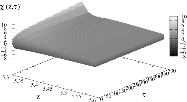
Figure 1: The growing mode solution for $\chi(z,\tau)$. We take $\beta=0.1$ and $H/\mu=100$. The brane is located at $z_{b}=5.3$.

Figure 2: The growing mode solution for $\chi(z,\tau)$ for the same parameters as in Fig. 1. Left: the profile of $\chi(z,\tau)$ in the bulk. The amplitude is normalised so that the amplitude on the brane is equal to 1. Right: behaviour of $\chi$ on the brane, $\chi(z_{b},\tau)$.

Figure 3: Left: The growing mode solution for $\xi(\tau)$ for the same parameters as in Fig. 1. Right: Comparison between the growing mode $\xi_{g}$ (solid line) and decaying mode $\xi_{d}$ (dotted line).

Figure 4: Behaviour of the Wronskian between the growing and decaying bound states, $\bar{W}(f_{g},f_{d})$.

III.2 Kaluza–Klein tower

The numerical results indicate that even at early times, there exists the bound states. In Refs. KLMW ; KMW , the behaviour of the bound states has been analyzed by performing the perturbative expansion in $\beta^{2}$. It was shown that, in terms of the Kaluza–Klein decomposition, the bound state is composed of an infinite ladder of modes with negative mass squared. Due to the excitation of the infinite ladder of the modes, the naive perturbation expansion in $\beta^{2}$ breaks down at early times KMW . In this paper, we derive the solutions without performing the perturbative expansion in $\beta^{2}$.

The bulk equation of motion for $\chi$, Eq. (32) is straightforward to solve. The solutions can be written in the form KLMW

$$\chi=\int d\nu\,B_{\nu}f_{\nu}(z)T_{\nu}(\tau)\,,$$ (56)

where $\nu$ is related to the conventional Kaluza–Klein mass as

$$\nu=\sqrt{\frac{9}{4}-\frac{m^{2}}{H^{2}}},$$ (57)

$\tau^{-1/2}T_{\nu}(\tau)$ is in general a linear combination of the Bessel function $J_{\nu}(\tau)$ and Neumann function $N_{\nu}(\tau)$, and $(\sinh z)^{-1/2}f_{\nu}(z)$ is a linear combination of the Legendre functions $P_{\nu-1/2}(\cosh z)$ and $Q_{\nu-1/2}(\cosh z)$. We are interested in the bound states for which $\chi$ vanishes as $\tau\to 0$ and/or $z\to\infty$, so we consider the solutions composed of the following mode functions:

$$T_{\nu}(\tau)=\tau^{1/2}J_{\nu}(\tau)\,,\qquad f_{\nu}(z)=\left(\frac{\sinh z}{\sinh z_{{}_{\rm b}}}\right)^{1/2}\frac{Q_{\nu-1/2}(\cosh z)}{Q_{\nu-1/2}(\cosh z_{{}_{\rm b}})}\,,$$ (58)

where $\mbox{Re}~{}\nu>0$. Our normalisation ensures $f_{\nu}(z_{{}_{\rm b}})=1$. We can then write the brane field $\xi$ in terms of the mode functions $T_{\nu}(\tau)$ as

$$\xi=\int d\nu\,C_{\nu}T_{\nu}(\tau)\,.$$ (59)

The brane equation of motion (42) and the junction condition (43) then reduce to two coupled difference equations relating the coefficients $B_{\nu}$ and $C_{\nu}$ entering Eqs. (56) and (59),

$$\frac{F_{\nu+1}}{2(\nu+1)}B_{\nu+1}+\frac{F_{\nu-1}}{2(\nu-1)}B_{\nu-1}=C_{\nu}\,,$$ (60)

$$\frac{(\nu+1)^{2}-1/4}{2(\nu+1)}C_{\nu+1}+\frac{(\nu-1)^{2}-1/4}{2(\nu-1)}C_{\nu-1}=-2\beta^{2}B_{\nu}\,,$$ (61)

where we use the shorthand

$$F_{\nu}=\frac{Q^{1}_{\nu-1/2}(\cosh z_{{}_{\rm b}})}{Q_{\nu-1/2}(\cosh z_{{}_{\rm b}})}\;.$$ (62)

We now derive two independent bound state solutions to these coupled equations.

To get a bound state we require that $B_{\nu}=0$ whenever $\mbox{Re}~{}\nu\leq 0$. It can be seen from Eqs. (60) and (61) that there are two such solutions: one for which $C_{2n-1/2}$ and $B_{2n+1/2}$ are non-vanishing only, and the other with non-zero values only of $C_{2n+1/2}$ and $B_{2n+3/2}$, where $n=0,1,2,\dots$. Importantly, we choose $C_{-1/2}$ real, then all $C_{2n-1/2}$ and $B_{2n+1/2}$ obtained from Eqs. (60) and (61) are real; the same is true for the second solution.

At late times, the modes with higher $n$ decay faster, thus the late time solutions are described by the lowest mode:

$$\chi_{g} = B_{1/2}f_{1/2}(z)T_{1/2}(\tau),\quad\xi_{g}=C_{-1/2}T_{-1/2}(\tau),$$

$$\chi_{d} = B_{3/2}f_{3/2}(z)T_{3/2}(\tau),\quad\xi_{d}=C_{1/2}T_{1/2}(\tau)\;,$$ (63)

where $C_{-1/2}$ and $C_{1/2}$ are arbitrary constants and according to (60)

$$B_{1/2}=\frac{C_{-1/2}}{F_{1/2}}\;,\quad B_{3/2}=\frac{3C_{1/2}}{F_{3/2}}\;.$$ (64)

We see that the solution that starts from $C_{-1/2}$ corresponds to the growing mode (45) with $A_{g}=C_{-1/2}\sqrt{2/\pi}$, while the solution that starts from $C_{1/2}$ corresponds to the decaying mode (47) with $A_{d}=C_{1/2}\sqrt{2/\pi}$. Hence, solving the recurrence equations (60) and (61) starting from $C_{-1/2}$ or $C_{1/2}$ is equivalent to evolving the late time bound state solutions backwards to obtain their early time behaviour. We have solved the recurrence relations numerically, the results are shown in Figs. 5 and 6. Using these solutions, we have checked that the solutions $\chi(\tau,z)$, $\xi(\tau)$ obtained by summing up the ladder of modes are in excellent agreement with the results of numerical simulations described in section III.1.

Figure 5: Solutions for $C_{\nu}$ with $\beta^{2}=0.1$. The growing mode solution with $C_{2n-1/2}$ is shown by $+$ and the decaying mode solution with $C_{2n+1/2}$ is shown by $\times$. We took $C_{1/2}=C_{-1/2}=1.$

Figure 6: Solutions for $C_{2n-1/2}$ and $B_{2n+1/2}$ for large $n$.

III.3 High energy limit: analytical treatment

From now on we will work in the high energy limit $H/\mu\gg 1$. In this limit one has

$$F_{\nu}\to-\left(\nu+\frac{1}{2}\right)\quad\text{as}\quad H/\mu\to\infty\,.$$ (65)

and the expression (58) for the mode function simplifies to

$$f_{\nu}(z)=e^{-\nu(z-z_{b})}.$$ (66)

In order to derive analytically the asymptotic behaviour of the bound state solutions at early times, $\tau\to\infty$, it is useful to have an asymptotic expansion for $B_{\nu}$ and $C_{\nu}$ for large $n$ or equivalently for large $\nu$. From the numerical solutions we find that the sequences $B_{2n+1/2}$ and $C_{2n-1/2}$ alternate in sign (and the same for the other solution) so we define new sequences

$$\overline{B}_{2n+1/2}=(-1)^{n+1}B_{2n+1/2}\,,\quad\overline{C}_{2n-1/2}=(-1)^{n}C_{2n-1/2}\,,$$ (67)

for the growing bound state and

$$\overline{B}_{2n+3/2}=(-1)^{n+1}B_{2n+3/2}\,,\quad\overline{C}_{2n+1/2}=(-1)^{n}C_{2n+1/2}\,,$$ (68)

for the decaying bound state. For large $\nu$, we can write the difference equations as

$$\overline{C}_{\nu} = \left[\frac{x-1/2}{2x}\overline{B}_{x}\right]_{x=\nu-1}^{x=\nu+1}\simeq\frac{d}{d\nu}\left(\overline{B}_{\nu}\right)\,,$$ (69)

$$-2\beta^{2}\overline{B}_{\nu} = \left[\frac{x^{2}-1/4}{2x}\overline{C}_{x}\right]_{x=\nu-1}^{x=\nu+1}\simeq\frac{d}{d\nu}\left(\nu\overline{C}_{\nu}\right)\,,$$ (70)

provided that $\overline{B}_{\nu}$ and $\overline{C}_{\nu}$ are smooth functions of $\nu$ whose derivatives vanish as $\nu\to\infty$. From Eqs. (69) and (70) it follows that the coefficients $\overline{B}_{\nu}$ satisfy the differential equation

$$\frac{d}{d\nu}\left(\nu\frac{d\overline{B}_{\nu}}{d\nu}\right)+2\beta^{2}\overline{B}_{\nu}=0\,,$$ (71)

to the leading order in $\nu^{-1}$, which has solutions

$$\overline{B}_{\nu}\propto Z_{0}\big{(}2\beta\sqrt{2\nu}\big{)}\,,$$ (72)

where $Z_{0}$ is a linear combination of the Bessel function of order 0,

$$Z_{0,i}\big{(}2\beta\sqrt{2\nu}\big{)}=A_{J,i}J_{0}\big{(}2\beta\sqrt{2\nu}\big{)}+A_{N,i}N_{0}\big{(}2\beta\sqrt{2\nu}\big{)},$$ (73)

where $i=g$ for the growing mode solution and $i=d$ for the decaying mode solution, and $A_{J,i}$ and $A_{N,i}$ are yet undetermined real constants, two for the growing mode and two for the decaying mode. The reality of $A_{J,i}$ and $A_{N,i}$ follows from the reality of $B_{\nu}$. From (60) we find, again to the leading order in $\nu^{-1}$,

$$\overline{C}_{\nu}=\frac{d\overline{B}_{\nu}}{d\nu}=-\beta\sqrt{\frac{2}{\nu}}\,Z_{1}\big{(}2\beta\sqrt{2\nu}\big{)}\,,$$ (74)

where $Z_{1}$ is the combination of $J_{1}$ and $N_{1}$ with the same coefficients $A_{J,i}$ and $A_{N,i}$ as in Eq. (73). In the large-$n$ asymptotics, the coefficients for the growing bound-state solution are thus

$$B_{2n+1/2}=(-1)^{n+1}Z_{0}\big{(}4\beta\sqrt{n}\big{)}\,,\qquad C_{2n-1/2}=(-1)^{n+1}\beta\,\frac{Z_{1}\big{(}4\beta\sqrt{n}\big{)}}{\sqrt{n}}\,.$$ (75)

In the same way, the decaying bound state has

$$B_{2n+3/2}=(-1)^{n+1}Z_{0}\big{(}4\beta\sqrt{n}\big{)}\,,\qquad C_{2n+1/2}=(-1)^{n+1}\beta\,\frac{Z_{1}\big{(}4\beta\sqrt{n}\big{)}}{\sqrt{n}}\,,$$ (76)

We have checked that the agreement between these asymptotic solutions and the numerical solutions of Eqs. (60) and (61) is excellent after we fit the two coefficients $A_{J,i}$ and $A_{N,i}$ for each mode.

To the zeroth order in $\beta^{2}$, the constants $A_{J,i}$ and $A_{N,i}$ can be expressed analytically through $C_{-1/2}$ (for the growing mode) and $C_{1/2}$ (for the decaying mode). Since for the growing mode $C_{\nu}$ is $O(\beta^{2})$ for $\nu>-1/2$, we can neglect $C_{\nu}$ with $\nu>-1/2$ in Eq. (60) for the this mode. Likewise, we can neglect $C_{\nu}$ with $\nu>1/2$ for the decaying mode. Then, as was first shown in KLMW , Eq. (60) can be solved as

$$B_{2n+1/2}=(-1)^{n}\left(2n+\frac{1}{2}\right)\frac{2}{F_{2n+1/2}}C_{-1/2},\quad B_{2n+3/2}=(-1)^{n}\left(2n+\frac{3}{2}\right)\frac{2}{F_{2n+3/2}}C_{1/2}.$$ (77)

Making use of the expression (65) valid in the high energy regime, we get for $n\gg 1$

$$B_{2n+1/2}=(-1)^{n+1}2C_{-1/2},\quad B_{2n+3/2}=(-1)^{n+1}2C_{1/2}.$$ (78)

Comparing with the non-perturbative solutions (76) and (75), we find that the perturbative solutions (78) are valid for $\beta\sqrt{n}\ll 1$. Taking the small argument limit of Eqs. (76) and (75), we obtain

$$A_{J,g}=2C_{-1/2},\quad A_{J,d}=2C_{1/2},\quad A_{N,g}=A_{N_{d}}=0,$$ (79)

at the zeroth order in $\beta^{2}$. The latter relations effectively provide matching between the late-time behaviour (63) and the early-time asymptotics which we are about to find. This matching, however, is valid to the zeroth order in $\beta^{2}$ only.

It should be emphasized that the perturbative approach breaks down for $\beta\sqrt{n}\gtrsim 1$. This is because, even if each $C_{\nu}$ with $\nu\neq\pm 1/2$ is $O(\beta^{2})$, the contribution to $B_{\nu}$ from $C_{\nu}$ in Eq. (60) is $O(n\times C_{\nu})\sim O(n\beta^{2})$. As we will see later, large-$n$ modes become dominant for large $\tau$. Then even for small $\beta^{2}$, the naive perturbation theory in $\beta$ breaks down at large $\tau$. This is in accord with Ref. KMW . For finite $\beta^{2}$, $A_{J,i}$ and $A_{N,j}$ are found from numerical solutions of Eqs. (60) and (61) and they are shown in Fig. 7.

Figure 7: Numerical solutions for the coefficients $A_{J,i}$ and $|A_{N,i}|^{2}/|A_{J,i}|^{2}$, defined in Eq. (73), for different values of $\beta^{2}$. We took $C_{1/2}=C_{-1/2}=1.$

Using the asymptotic expressions for the coefficients given in Eqs. (76) and (75), we can approximate the solutions at $z-z_{b}\ll 1$ by

$$\chi_{g}(\tau,z) \simeq \sum_{n}(-1)^{n+1}Z_{0}\big{(}4\beta\sqrt{n}\big{)}\sqrt{\tau}J_{2n+1/2}(\tau)e^{-2n(z-z_{b})},$$

$$\chi_{d}(\tau,z) \simeq \sum_{n}(-1)^{n+1}Z_{0}\big{(}4\beta\sqrt{n}\big{)}\sqrt{\tau}J_{2n+3/2}(\tau)e^{-2n(z-z_{b})}\,.$$ (80)

For large $\tau$, the sums over the modes can be evaluated explicitly. First we use the asymptotic expression for the Bessel functions,

$$J_{\nu}(\tau)\simeq\sqrt{\frac{2}{\pi\nu\tan\theta}}\cos\big{(}\nu\tan\theta-\nu\theta-\pi/4\big{)},$$ (81)

where $\cos\theta=\nu/\tau$, see Ref. GradRyz . The sums are dominated by the modes for which $n/\tau\ll 1$ but $n^{2}/\tau\gg 1$. In this regime the asymptotic expression simplifies to

$$J_{n+1/2}(\tau)=\sqrt{\frac{2}{\pi\tau}}\cos\big{(}\tau+n^{2}/(2\tau)-n\pi/2-\pi/2\big{)}\,.$$ (82)

The standard large-argument asymptotic form GradRyz for the Bessel function $Z_{0}$ in Eq. (76) enables one to approximate the sums in Eqs. (III.3) and (80) as

$$\chi_{g} \propto (A_{J,g}+iA_{N,g})\int dn\,n^{-1/4}\,\exp\left(-2n(z-z_{b})-4i\beta\sqrt{n}+i\tau+2in^{2}\tau^{-1}\right)+c.c.\,,$$

$$\chi_{d} \propto (A_{J,d}+iA_{N,d})\int dn\,n^{-1/4}\,\exp\left(-2n(z-z_{b})-4i\beta\sqrt{n}+i\tau+2in^{2}\tau^{-1}-\frac{\pi}{2}i\right)+c.c.\,,$$ (83)

where we keep only the terms that give dominant contributions to the integrals (see below). The phase difference of $\pi/2$ between the growing mode and decaying mode solutions comes from the fact that the growing mode and decaying mode solutions contain $J_{2n+1/2}$ and $J_{2n+3/2}$, respectively. At large $\tau$ (early times) these integrals are saturated by modes with large $n$. This means, in particular, that we cannot truncate the ladder of modes if we wish to describe the early time behaviour KMW . The leading-order contribution comes from the saddle point at

$$n_{{}_{\rm saddle}}=\frac{1}{2^{2/3}}\beta^{2/3}\tau^{2/3}-\frac{i}{3}(z-z_{b})\tau\,.$$ (84)

The integrals in Eq. (III.3) can thus be approximated as

$$\chi_{g} \propto (A_{J,g}+iA_{N,g})\tau^{1/3}\exp\left(i\tau-\frac{3i}{2^{1/3}}\beta^{4/3}\tau^{1/3}-2^{1/3}\beta^{2/3}\tau^{2/3}(z-z_{b})+\frac{i}{3}\tau(z-z_{b})^{2}\right)+c.c.\,,$$

$$\chi_{d} \propto (A_{J,d}+iA_{N,d})\tau^{1/3}\exp\left(i\tau-\frac{3i}{2^{1/3}}\beta^{4/3}\tau^{1/3}-2^{1/3}\beta^{2/3}\tau^{2/3}(z-z_{b})+\frac{i}{3}\tau(z-z_{b})^{2}-\frac{\pi}{2}i\right)+c.c.\,.$$ (85)

Note that at large $\tau$, these wave functions are localized in a narrow region in the bulk, $z-z_{b}\sim(\beta\tau)^{-3/2}\ll 1$, as we anticipated when writing Eq. (III.3). The terms omitted in Eq. (III.3) do not have saddle points near the semi-axis of positive $n$ and thus give the contributions which are exponentially suppressed as compared to Eq. (85). In the same way we can find the asymptotic behaviour of $\xi$,

$$\xi_{g} \propto (A_{J,g}+iA_{N,g})\exp\left(i\tau-\frac{3i}{2^{1/3}}\beta^{4/3}\tau^{1/3}\right)+c.c\,,$$

$$\xi_{d} \propto (A_{J,d}+iA_{N,d})\exp\left(i\tau-\frac{3i}{2^{1/3}}\beta^{4/3}\tau^{1/3}-\frac{\pi}{2}i\right)+c.c\,.$$ (86)

These asymptotic expressions nicely explain the behaviour of solutions at early times ($\tau\gg 1$) obtained in our numerical simulations. We see that the amplitude of $\chi(z_{b},\tau)$ increases as $\chi(z_{b},\tau)\propto\tau^{1/3}$ while the amplitude of $\xi$ tends to a constant at large $\tau$. At the same time, $\chi(z,\tau)$ is increasingly dominated by large-$n$ modes and becomes more and more closely bound to the brane at large $\tau$. This behaviour ensures that the Wronskian for $\chi$, given in Eq. (55), is conserved at late times. We also notice that the phase difference between the growing mode and decaying mode solutions is approximately equal to $\pi/2$, provided that $A_{J,i}\gg A_{N,i}$. As we saw above, the latter inequality is indeed valid at small $\beta^{2}$, so the pattern shown in the right panel of Fig. 3 also has its analytical explanation.

To conclude this section, we notice that at early times, the original coupled system Eqs. (32), (42) and (43) may be treated within the WKB approximation. This is done in Appendix A. The WKB analysis is in prefect agreement with the results Eqs. (85) and (86).

IV The quantum amplitude

In the preceding section, we have found the early time behaviour of the bound state solutions, Eqs. (85) and (86). For finite $\beta^{2}$ they are parameterized by the real coefficients $A_{J,i}$ and $A_{N,i}$ where $i=g,d$ for the growing and decaying bound state solution, respectively. These coefficients can be found numerically, see Fig. 7. Importantly, the expressions (85) and (86) show that despite the complicated behaviour of the bound states at early times, the division of solutions into positive- and negative-frequency parts is well defined as $\tau\to\infty$. This is also clear from the WKB analysis, see Appendix A. Thus, as in the familiar four-dimensional case, we can straightforwardly quantise the perturbations and define the vacuum state on small scales (early times) to determine the final amplitude of the inflaton fluctuations. We follow the method developed in Refs wronskian1 ; wronskian2 to relate the amplitude of the growing mode solution to the creation and annihilation operators. In principle, this method involves the construction of properly normalised positive- and negative-frequency solutions at early times and the evaluation of the inner product (Wronskian) between these solutions and the bound states. However, there is a short-cut: all we need are the values of the real coefficients $A_{J,i}$ and $A_{N,i}$. We first explain this short-cut by making use of the familiar four-dimensional example, and then proceed to the brane-world model. In this section, we restore $k$, but we are still working with redefined time $\tau\to-\tau$.

IV.1 Four-dimensional case

Let us begin with the standard four-dimensional case. At the first order in the slow-roll parameters, the equation for $u$ is

$$u_{,\tau\tau}+k^{2}u-\frac{1}{\tau^{2}}(2+6\epsilon_{{}_{H}}-3\eta_{{}_{H}})u=0.$$ (87)

In the same way as in Eq. (41), we define

$$\xi=u_{,\tau}+(1+2\epsilon_{{}_{H}}-\eta_{{}_{H}})\frac{u}{\tau}.$$ (88)

The equation for $\xi$ is

$$\xi_{,\tau\tau}+k^{2}\xi-\frac{2\epsilon_{{}_{H}}-\eta_{{}_{H}}}{\tau^{2}}\xi=0,$$ (89)

The Wronskian is defined as

$$W(\xi^{*},\xi)=\frac{1}{k^{2}}(\xi^{*}\xi_{,\tau}-\xi\xi^{*}_{,\tau}).$$ (90)

Neglecting $k^{2}$ in Eq. (89), one obtains the growing mode and the decaying mode solutions at late times, $\tau\to 0$,

$$\xi_{g}\to(k\tau)^{1/2-\nu}2^{\nu}\frac{1}{\Gamma(-\nu+1)},\quad\xi_{d}\to(k\tau)^{1/2+\nu}2^{-\nu}\frac{1}{\Gamma(\nu+1)}.$$ (91)

where $\nu=1/2+2\epsilon_{{}_{H}}-\eta_{{}_{H}}$ and we included numerical factors for later convenience. We are interested in quantum field which behaves at late times as

$$\hat{\xi}\to\hat{Z}\xi_{g},$$ (92)

where $\hat{Z}$ is a time-independent quantum operator. This field is quantised on small scales where we can expand $\hat{\xi}$ in terms of negative- and positive-frequency modes,

$$\hat{\xi}=\hat{a}\varphi^{(-)}+\hat{a}^{\dagger}\varphi^{(+)},$$ (93)

where $\hat{a}$ and $\hat{a}^{\dagger}$ are annihilation and creation operators, respectively, which define the vacuum

$$\hat{a}|0\rangle=0.$$ (94)

We should note that due to the redefinition of time $\tau\to-\tau$, the definitions of the negative- and positive-frequency functions are $\varphi^{(-)}\propto e^{ik\tau}$ and $\varphi^{(+)}\propto e^{-ik\tau}$. The mode functions should be normalised as

$$W(\varphi^{(-)},\varphi^{(+)})=-i\;.$$ (95)

The latter condition ensures the canonical commutational relation between $\xi$ and its conjugate momentum.

Our aim is to express $\hat{Z}$ in terms of $\hat{a}$ and $\hat{a}^{\dagger}$. We exploit the constancy of the Wronskian for this purpose. At late times, $\hat{Z}$ can be related to the Wronskians,

$$\hat{Z}=\frac{W(\hat{\xi},\xi_{d})}{W(\xi_{g},\xi_{d})}.$$ (96)

Here $W(\xi_{g},\xi_{d})$ can be calculated using the late time solutions (91) for $\xi_{g}$ and $\xi_{d}$,

$$W(\xi_{g},\xi_{d})=\frac{1}{k}\left(\frac{2}{\pi}\right)\sin(\nu\pi).$$ (97)

On the other hand, $W(\hat{\xi},\xi_{d})$ can be calculated at early times. For this purpose, we expand the growing mode and the decaying mode solutions in $\varphi^{(+)}$ and $\varphi^{(-)}$ at early times,

$$\xi_{g}=c_{g}\varphi^{(-)}+c_{g}^{*}\varphi^{(+)},\quad\xi_{d}=c_{d}\varphi^{(-)}+c_{d}^{*}\varphi^{(+)}.$$ (98)

Then, $W(\hat{\xi},\xi_{d})$ is calculated as

$$W(\hat{\xi},\xi_{d})=-i\left(\hat{a}c_{d}^{*}-\hat{a}^{\dagger}c_{d}\right).$$ (99)

As usual, the operator $\hat{Z}$ corresponds to the Gaussian random field, fully characterised by the vacuum expectation value of its square. The latter is evaluated as

$$\langle\hat{Z}^{\dagger}\hat{Z}\rangle=k^{2}\left(\frac{\pi}{2}\right)^{2}|c_{d}|^{2}(\sin\nu\pi)^{-2}.$$ (100)

Thus the problem reduces to finding $c_{d}$, which is the expansion coefficient for the decaying mode solution.

Now, the trick is that we do not need to know the precise expressions for $\varphi^{(\pm)}$ to determine $|c_{d}|$. Indeed, by solving for the growing mode and decaying mode backwards, it is possible, at least in principle (and in practice in the four-dimensional example), to derive the early-time solutions for $\xi_{g}$, $\xi_{d}$. In the four-dimensional case they are

$$\xi_{g}=N_{g}\cos(k\tau+\Delta_{g}),\quad\xi_{d}=N_{d}\cos(k\tau+\Delta_{d}).$$ (101)

This immediately impies that the positive- and negative-frequency modes have the form

$$\varphi^{(\pm)}=|\varphi|e^{\mp i\delta}e^{\mp ik\tau}\,,$$ (102)

where the normalisation factor $|\varphi|$ may be found from (95), but will not be needed in what follows, and $\delta$ is some phase (which is irrelevant in the four-dimensional case). Comparing Eqs. (98) and (101), we get

$$\frac{|c_{d}|}{|c_{g}|}=\frac{N_{d}}{N_{g}},\quad\mbox{Arg}\,c_{g}-\mbox{Arg}\,c_{d}\equiv\delta_{g}-\delta_{d}=\Delta_{g}-\Delta_{d}.$$ (103)

The additional information on $c_{d},c_{g}$ and $|\delta_{d}-\delta_{g}|$ can be obtained from the Wronskian $W(\xi_{g},\xi_{d})$. In terms of $c_{g}$ and $c_{d}$, the Wronskian is calculated as

$$W(\xi_{g},\xi_{d})=2|c_{g}||c_{d}||\sin(\delta_{g}-\delta_{d})|\,.$$ (104)

Now we can use Eq. (97) together with Eqs (103) and (104) to obtain $|c_{d}|^{2}$ in terms of $N_{d}/N_{g}$ and $|\Delta_{g}-\Delta_{d}|$,

$$|c_{d}|^{2}=\frac{1}{2}\frac{N_{d}}{N_{g}}\frac{1}{|\sin(\Delta_{g}-\Delta_{d})|}\frac{1}{k}\left(\frac{2}{\pi}\right)\sin\nu\pi.$$ (105)

Thus, the quantity $|c_{d}|^{2}$ entering (100) is expressed in terms of the ratio $N_{d}/N_{g}$ of the amplitudes and difference $(\Delta_{g}-\Delta_{d})$ of the phases of the decaying and growing modes evolved back in time.

In the four-dimensional case, the growing mode and the decaying mode solutions are

$$\xi_{g}=(k\tau)^{1/2}J_{-\nu}(k\tau),\quad\xi_{d}=(k\tau)^{1/2}J_{\nu}(k\tau),$$ (106)

At late times, $\tau\to 0$, they have the form (91), while at early times, $k\tau\gg 1$, the solutions become

$$\xi_{g}\to\sqrt{\frac{2}{\pi}}\cos\left(k\tau+\frac{1}{2}\nu\pi-\frac{1}{4}\pi\right),\quad\xi_{d}\to\sqrt{\frac{2}{\pi}}\cos\left(k\tau-\frac{1}{2}\nu\pi-\frac{1}{4}\pi\right).$$ (107)

We thus find

$$\frac{N_{d}}{N_{g}}=1,\quad\Delta_{g}-\Delta_{d}=\nu\pi.$$ (108)

Then $|c_{d}|^{2}$ is obtained as

$$|c_{d}|^{2}=\frac{1}{2k}\left(\frac{2}{\pi}\right),$$ (109)

and the expectation value for $\hat{Z}$ squared is given by

$$\langle\hat{Z}^{\dagger}\hat{Z}\rangle=\frac{k\pi}{4}(\sin\nu\pi)^{-2}.$$ (110)

In this way, from the solutions for the growing and decaying modes, we can determine the quantum amplitude of the fluctuations. We note in parenthesis that the slow-roll corrections do not affect the value of $|c_{d}|$ in the four-dimensional case. This is because the slow-roll effects do not play any role at early times in Eq. (89).

The quantity that is related to observables is the comoving curvature perturbation,

$${\cal R}_{c}=-\frac{H}{a\dot{\phi}}u.$$ (111)

Using the result for the quantum expectation value for $\hat{Z}^{\dagger}\hat{Z}$, Eq. (110), and the late-time asymptotics (91), we get from (88) at $k\tau\ll 1$

$$\langle u^{2}\rangle^{1/2}\to 2^{2\epsilon_{{}_{H}}-\eta_{{}_{H}}}\frac{\Gamma(3/2+2\epsilon_{{}_{H}}-\eta_{{}_{H}})}{\Gamma(3/2)}\frac{1}{\sqrt{2k}}(k\tau)^{-1-2\epsilon_{{}_{H}}+\eta_{{}_{H}}}.$$ (112)

Expanding the Gamma function in Eq. (112), we find

$$\langle u^{2}\rangle^{1/2}\to\Big{\{}1+(2\epsilon_{{}_{H}}-\eta_{{}_{H}})(2-\gamma-\ln 2)\Big{\}}\frac{1}{\sqrt{2k}}(k\tau)^{-1-2\epsilon_{{}_{H}}+\eta_{{}_{H}}}\,.$$ (113)

Here we have used the formula for the psi function

$$\psi(3/2)\equiv\frac{\Gamma^{\prime}(3/2)}{\Gamma(3/2)}=2-\gamma-2\ln 2,$$ (114)

where $\gamma$ is the Euler constant. The power spectrum of the curvature perturbation is then given by

$${\cal{P}}_{{\cal R}_{c}}(k)=\frac{k^{3}}{2\pi^{2}}\langle{\cal R}_{c}^{2}\rangle=\frac{k^{3}}{2\pi^{2}}\left(\frac{H}{a\dot{\phi}}\right)^{2}\langle u^{2}\rangle.$$ (115)

Using the fact that conformal time is given, up to the first order in slow-roll parameters, by

$$\tau=\frac{1}{aH}(1+\epsilon_{{}_{H}}),$$ (116)

one finds the power spectrum of the curvature perturbation,

$${\cal{P}}_{{\cal R}_{c}} = \left(\frac{H}{\dot{\phi}}\right)^{2}\left(\frac{H}{2\pi}\right)^{2}\Big{[}1+2S(\epsilon_{{}_{H}},\eta_{{}_{H}})\Big{]},\quad S(\epsilon_{{}_{H}},\eta_{{}_{H}})=(2\epsilon_{{}_{H}}-\eta_{{}_{H}})(2-\ln 2-\gamma)-\epsilon_{{}_{H}}\,,$$ (117)

where $S$ is known as the Stewart–Lyth correction SL .

IV.2 Brane-world case

We now apply the method presented in the preceding subsection to the brane-world case. The late time behaviour of $\xi$ is the same as in the four-dimensional case: at late times we have

$$\hat{\xi}\to\hat{Z}\xi_{g}.$$ (118)

We expand the quantum operators $\hat{\xi}$ and $\hat{\chi}$ at early times as

$$\hat{\xi} = \hat{a}\varphi^{(-)}+\hat{a}^{\dagger}\varphi^{(+)},$$

$$\hat{\chi} = \hat{a}\phi^{(-)}+\hat{a}^{\dagger}\phi^{(+)},$$ (119)

where $\varphi^{(\pm)}$ and $\phi^{(\pm)}$ are the positive and negative frequency solutions to the coupled equations, obeying the normalisation condition

$$W(f^{(-)},f^{(+)})=-i,$$ (120)

where $f^{(\pm)}=(\varphi^{(\pm)},\phi^{(\pm)})$, and the Wronskian has precisely the form (44). This normalisation ensures the canonical quantisation conditions for the fields, as is shown in Appendix B.

The growing mode solution and the decaying mode solution are also expanded as

$$\xi_{i}\to c_{i}\varphi^{(-)}+c_{i}^{*}\varphi^{(+)},\quad\chi_{i}\to c_{i}\phi^{(-)}+c_{i}^{*}\phi^{(+)},$$ (121)

where $i=g,d$. At late times, the contribution from $\chi$ to the Wronskian can be neglected and the dominant contribution comes from the lowest mode in the ladder of the modes, Eq. (63),

$$\xi_{g}=(k\tau)J_{-1/2}(k\tau),\quad\xi_{d}=(k\tau)J_{1/2}(k\tau),$$ (122)

where we set $C_{1/2}=C_{-1/2}=1$. In this way we obtain the Wronskian,

$$W(f_{g},f_{d})=\frac{1}{k}\frac{2}{\pi}.$$ (123)

Then, as in the four-dimensional case, the expectation value of the quantum operator $\hat{Z}^{\dagger}\hat{Z}$ is calculated as

$$\langle\hat{Z}^{\dagger}\hat{Z}\rangle=k^{2}\left(\frac{\pi}{2}\right)^{2}|c_{d}|^{2}.$$ (124)

The virtue of the approach outlined above is that it works even in cases when the early-time solutions have complicated form. In the brane-world case, the positive- and negative-frequency solutions can be read off from Eqs. (85) and (86), and they indeed are rather complicated. Nevertheless, the above argument goes through, and we find, in exact analogy with the result (105),

$$|c_{d}|^{2}=\frac{1}{2}\frac{N_{d}}{N_{g}}\frac{1}{|\sin(\Delta_{g}-\Delta_{d})|}\frac{1}{k}\left(\frac{2}{\pi}\right),$$ (125)

where

$$\frac{|N_{d}|^{2}}{|N_{g}|^{2}}=\frac{A_{J,d}^{2}+A_{N,d}^{2}}{A_{J,g}^{2}+A_{N,g}^{2}},\quad\Delta_{g}-\Delta_{d}=\frac{\pi}{2}+\left[\arctan\frac{A_{N,g}}{A_{J,g}}-\arctan\frac{A_{N,d}}{A_{J,d}}\right].$$ (126)

As a cross check, let us show that the standard four-dimensional result is recovered at the zeroth order in $\beta^{2}$. At this order, the solutions for $A_{J,i}$ and $A_{N,i}$ are given by Eq. (79). Then Eq. (126) yields

$$\frac{|N_{d}|^{2}}{|N_{g}|^{2}}=1,\quad\Delta_{g}-\Delta_{d}=\frac{\pi}{2},$$ (127)

and we get

$$|c_{d}|^{2}=\frac{1}{2k}\left(\frac{2}{\pi}\right),$$ (128)

which agrees with the four-dimensional result, Eq. (109).

For finite $\beta^{2}$ we use numerical solutions for $A_{J,i}$ and $A_{N,i}$ shown in Fig. 7 to evaluate $N_{d}/N_{g}$ and $(\Delta_{g}-\Delta_{d})$. The results are presented in Fig. 8. Using these numerical results, we obtain the expectation value of interest,

$$\langle\hat{Z}^{\dagger}\hat{Z}\rangle=\frac{k\pi}{4}\Big{[}1+K(\beta^{2})\Big{]}\,,$$ (129)

where $K(\beta^{2})$ is shown in Fig. 9. As is seen from Fig. 9, $K(\beta^{2})\sim O(\beta^{2})\sim O(\epsilon_{{}_{H}})$.

Figure 8: Numerical solutions for $|N_{d}|/|N_{g}|$ and $|\Delta_{g}-\Delta_{d}-\pi/2|$.

Figure 9: Numerical solutions for $K(\beta^{2})$.

IV.3 Amplitude of curvature perturbations

Finally, the amplitude of the comoving curvature perturbations is calculated using Eqs. (51) and (46). At late times, $\hat{\xi}$ behaves as

$$\hat{\xi}=\hat{Z}\sqrt{\frac{2}{\pi}}.$$ (130)

Then, comparing this with Eq. (46), we find the amplitude of $A_{g}$,

$$\langle A_{g}^{2}\rangle=\frac{1}{k^{4}}\frac{2}{\pi}\langle\hat{Z}^{\dagger}\hat{Z}\rangle=\frac{1}{2k^{3}}\Big{[}1+K(\beta^{2})\Big{]}.$$ (131)

Using Eq. (46), the spectrum of the curvature perturbations is evaluated as

$${\cal{P}}_{{\cal R}_{c}} = \left(\frac{H}{\dot{\phi}}\right)^{2}\left(\frac{H}{2\pi}\right)^{2}\Big{[}1+K(\beta^{2})\Big{]}.$$ (132)

We should note that we did not take into account the standard slow-roll corrections at the super-horizon scales in this calculation. The correction $K(\beta^{2})$ is solely due to the coupling between the inflaton and the bulk metric perturbations. Although the mode functions are significantly affected by this coupling at early times, the final correction to the quantum amplitude at late times is suppressed by the slow-roll parameter even in the high energy regime.

As the correction $K(\beta^{2})$ is of the same order as the usual slow-roll corrections, we should also take into account the corrections to the amplitude at the superhorizon scales. Since $K(\beta^{2})$ is already the first-order correction, the slow-roll corrections to $K(\beta^{2})$ are of higher order. Then we just need to add the Stewart–Lyth correction. Indeed, neglecting the coupling to the bulk metric perturbations that is already first order in the slow-roll parameter, the equation for $u$ is given by

$$u_{,\tau\tau}+k^{2}u-\frac{1}{\tau^{2}}(2+6\epsilon_{{}_{H}}-3\eta_{{}_{H}})u=0.$$ (133)

We find that this is exactly the same as in the four-dimensional case. Thus, the Stewart–Lyth correction is precisely the same as well; this was first shown in Ref. RL . Then at the first order in slow-roll, we get the final result

$${\cal{P}}_{{\cal R}_{c}} = \left(\frac{H}{\dot{\phi}}\right)^{2}\left(\frac{H}{2\pi}\right)^{2}\Big{[}1+K(\beta^{2})+2S(\epsilon_{{}_{H}},\eta_{{}_{H}})\Big{]}\,,$$ (134)

where $S=(2\epsilon_{{}_{H}}-\eta_{{}_{H}})(2-\ln 2-\gamma)-\epsilon_{{}_{H}}$ is the Stewart–Lyth correction. Fig. 10 shows the complete first order corrections in the brane-world model at high energies, $H\gg\mu$, compared with the Stewart–Lyth corrections.

Figure 10: First order corrections $2S(\epsilon_{{}_{H}},\eta_{{}_{H}})+K(\beta^{2})$ in the high energy regime $H\gg\mu$, compared with $2S(\epsilon_{{}_{H}},\eta_{{}_{H}})$ for $\eta_{{}_{H}}=0.1$ (left) and $\eta_{{}_{H}}=0.01$ (right).

V Conclusions

In this paper, we performed the quantisation of the inflaton perturbations during slow-roll inflation driven by an inflaton confined to a brane in the Randall-Sundrum brane world-model. The slow-roll dynamics leads to a finite coupling between the inflaton fluctuations on the brane and metric perturbations in the bulk. We first studied the effect of this coupling at the first order in the slow-roll expansion by keeping the coupling term while neglecting all other slow-roll corrections. This enabled us to deal with five-dimensional perturbations around the de Sitter brane for which the bulk wave equation is separable and solutions can be described as sums of bulk modes. At late times there exists bound states with single bulk modes, and the growing bound state determines the final amplitude of the comoving curvature perturbation on large scales. The continuum modes were shown to be orthogonal to the bound state in the sense that the Wronskian between them vanishes; furthermore, the continuum modes decay away at late times. Thus we could neglect the continuum modes in our analysis.

We evolved this late time bound state backwards numerically to find its early time behaviour. It was shown that the behaviour of the inflaton fluctuations is significantly affected by its coupling to an infinite tower of bulk modes, even at the first order in the slow-roll approximation. Asymptotically, the amplitude of $\xi$, that describes the inflaton perturbations on the brane, becomes constant while the amplitude of $\chi$, that describes the bulk metric perturbations, increases on the brane at early times. It was also found that $\chi$ is more and more concentrated near the brane at early times, becoming dominated by modes with large (and negative) Kaluza–Klein mass-squared. We found that it is possible to reproduce these numerical solutions by the summation of the infinite ladders of modes. The growing mode and decaying mode solutions have different ladders of modes, which leads to a phase shift between them. The infinite sum of the modes can be evaluated using a saddle point method and analytic formula for the asymptotic solutions was derived.

We then performed the quantisation of the bound state. We developed a scheme where the quantum amplitude of the perturbations can be derived by finding the early time behaviour of the growing mode and the decaying mode. In this method, the constancy of the Wronskian is exploited to connect the quantum operator at late times to the creation and annihilation operators defined at early times, without the explicit analysis of the early-time positive- and negative-frequency functions and the calculation of the Bogoliubov coefficients. This method was applied to the standard four-dimensional case to re-derive the Stewart–Lyth correction, which arises from corrections to the field evolution after horizon exit. We then applied this method to our brane-world model. In this case, there is a correction that arises from the modified solutions for the perturbations on small scales. Thus, this correction is due to the coupling of the inflaton to the bulk metric perturbations. Despite the fact that the behaviour of perturbations on small scales is qualitatively different due to this coupling, it was found that particle production is suppressed by the smallness of the coupling. The correction to the final amplitude was thus shown to be of the order of the slow-roll parameter, $\epsilon_{{}_{H}}$, even in the high energy regime.

Because the effect of the mixing between the brane inflaton fluctuations and the bulk metric perturbations is of the first order in the slow-roll parameter, the complete first order corrections consist of the correction $K(\beta^{2})$ coming from the brane-bulk mixing and the Stewart–Lyth correction $S(\epsilon_{{}_{H}},\eta_{{}_{H}})$, which was shown to have the same form as in the four-dimensional case. Fig. 10 is our main result showing the complete first order corrections in the brane-world model.

In four-dimensional general relativity the corrections to the evolution of inflaton fluctuations that arise at the first order in the slow-roll parameters can be neglected for wavelengths much smaller than the Hubble scale. Thus, the vacuum fluctuations on sub-horizon scales are essentially the same as those of a massless field in the de Sitter space-time Mukhanov . The only change in the amplitude of quantum fluctuations comes from the modification of evolution on super-horizon scales, leading to the familiar Stewart–Lyth correction SL .

By contrast, in the brane world the coupling between the inflaton fluctuations and bulk metric perturbations that arises at the first order in the slow-roll parameters leads to a radically different picture of the bound sates at early times compared with the zeroth-order solution. Short wavelength inflaton fluctuations do not decouple in the high energy regime ($H\gg\mu$) from the bulk metric perturbations and support an infinite tower of bulk modes, which become increasingly dominated by large-$n$ modes on small scales. Nonetheless, the mixing between positive- and negative-frequency modes is absent in the sub-horizon regime, while additional mixing near the horizon crossing is suppressed by slow-roll parameters, so the final correction to the amplitude of fluctuations on super-horizon scales is again first order in the slow-roll parameters.

Appendix A WKB approximation for early-time solution

Let us consider early times, i.e., large $\tau$. In this case we can find the bound state solutions to the coupled system of equations (32), (42) and (43) by making use of the WKB approximation. Using the rescaling given in Eq. (52) we approximate the solutions by

$$\xi=A(\tau)\exp(iS_{\xi}(\tau))\,,\qquad\chi=B(\tau,z)\exp(iS_{\chi}(\tau,z))\,,$$ (135)

where $A$ and $B$ are slowly varying functions but the exponential factors are varying rapidly. Consistency with the brane equation of motion (42) requires that

$$S_{\xi}(\tau)=S_{\chi}(\tau,z_{{}_{\rm b}})=S_{{}_{\rm b}}(\tau)\,.$$ (136)

In the WKB regime and in the high-energy limit, Eqs. (42) and (43) reduce to

$$\left(-\left(\frac{\partial S_{{}_{\rm b}}}{\partial\tau}\right)^{2}+1\right)A=-\frac{2\beta^{2}}{\tau}B_{{}_{\rm b}}\,,$$ (137)

$$i\left[\frac{\partial S_{\chi}}{\partial z}\right]_{{}_{\rm b}}B_{{}_{\rm b}}=\tau A\,.$$ (138)

From these equations we obtain the boundary condition for $S_{\chi}$,

$$\left(-\left(\frac{\partial S_{{}_{\rm b}}}{\partial\tau}\right)^{2}+1\right)\left[\frac{\partial S_{\chi}}{\partial z}\right]_{{}_{\rm b}}=2i\beta^{2}\,.$$ (139)

Let us also write the equation of motion for $\chi$, Eq. (32), at the boundary,

$$-\left(\frac{\partial S_{{}_{\rm b}}}{\partial\tau}\right)^{2}+1+\frac{1}{\tau^{2}}\left[\frac{\partial S_{\chi}}{\partial z}\right]^{2}_{{}_{\rm b}}=0\,.$$ (140)

The latter two equations give

$$\left(\frac{\partial S_{{}_{\rm b}}}{\partial\tau}\right)^{2}=1-\left(\frac{2\beta^{2}}{\tau}\right)^{2/3}\,,\qquad\left[\frac{\partial S_{\chi}}{\partial z}\right]_{{}_{\rm b}}=i2^{1/3}\beta^{2/3}\tau^{2/3}\,.$$ (141)

One can use this approach to solve for $S_{\chi}$ as a Taylor series about the brane position. The next derivative is

$$\left[\frac{\partial^{2}S_{\chi}}{\partial z^{2}}\right]_{{}_{\rm b}}=\frac{2}{3}\tau\,,$$ (142)

and so on. Note that this solution indeed satisfies the applicability conditions for the WKB approximation.

We can obtain the amplitudes $A$ and $B$ in a similar way by using the next order of the WKB approximation, finding that

$$A=\text{const}\,,\qquad B_{{}_{\rm b}}=\text{const}\cdot\tau^{1/3}\,.$$ (143)

Note that the amplitude of $\xi$ is constant but the amplitude of $\chi$ increases like $\tau^{1/3}$. The expansion near the brane gives

$$\chi(\tau,z)\propto\tau^{1/3}\,e^{-2^{1/3}\beta^{2/3}\tau^{2/3}(z-z_{b})}\,e^{-iS_{{}_{\rm b}}}\,.$$ (144)

This expression implies, in particular, that the contribution from the small-$z$ region to the normalisation integral

$$\int dx\,(\chi^{*}\chi_{,\tau}-c.c.),$$ (145)

is constant in $\tau$. The asymptotic solution Eq. (144) agrees with the solution obtained in Section III.B, Eq. (85).

Appendix B quantisation condition for coupled system

We normalised the positive- and negative-frequency modes as

$$W(f^{(-)},f^{(+)})=\frac{1}{k^{2}}(\varphi^{(-)}\varphi_{,\tau}^{(+)}-\varphi^{(+)}\varphi_{,\tau}^{(-)})+\frac{1}{3\kappa_{5}^{2}}\int_{z_{b}}^{\infty}dz(\phi^{(-)}\phi^{(+)}_{,\tau}-\phi^{(+)}\phi^{(-)}_{,\tau})=-i.$$ (146)

We justify this as follows. In terms of $\xi$ and $\chi$, the quadratic action is given by

$$S = \frac{1}{2k^{2}}\int d\tau(\xi_{,\tau}^{2}-k^{2}\xi^{2})+\frac{1}{6\kappa_{5}^{2}}\int^{\infty}_{z_{b}}dzd\tau\left(\chi_{,\tau}^{2}-k^{2}\chi^{2}-\frac{\chi^{\prime 2}+(U(z)-2H^{2})\chi^{2}}{(H\tau)^{2}}\right)$$ (147)

$$- \frac{\dot{\phi}}{3H}\int d\tau\frac{1}{\tau}\chi\xi+\frac{1}{12\kappa_{5}^{2}}\left(\frac{N^{\prime}}{N}\right)_{{}_{\rm b}}\int d\tau\frac{\chi^{2}}{(H\tau)^{2}}.$$

Therefore, the conjugate momenta are

$$\pi_{\xi}=-\frac{\xi_{,\tau}}{k^{2}},\quad\pi_{\chi}=-\frac{1}{3\kappa_{5}^{2}}\chi_{,\tau},$$ (148)

where the minus sign comes from the redefinition of time $\tau\to-\tau$. From the expansions of the fields in terms of $\hat{a}$ and $\hat{a}^{\dagger}$,

$$\xi = \hat{a}\varphi^{(-)}+\hat{a}^{\dagger}\varphi^{(+)},$$

$$\chi = \hat{a}\phi^{(-)}+\hat{a}^{\dagger}\phi^{(+)},$$ (149)

we can express $\hat{a}$ and $\hat{a}^{\dagger}$ as

$$W(f^{(-)},f)=-i\hat{a}^{\dagger},\quad W(f^{(+)},f)=i\hat{a}.$$ (150)

Then the commutation relation between $\hat{a}$ and $\hat{a}^{\dagger}$ is calculated as

$$[\hat{a},\hat{a}^{\dagger}] = [W(f^{(+)},f),W(f^{(-)},f)]$$ (151)

$$= \frac{1}{k^{2}}(\varphi^{(-)}\varphi_{,\tau}^{(+)}-\varphi^{(+)}\varphi_{,\tau}^{(-)})[\xi,\pi_{\xi}]+\frac{1}{3\kappa_{5}^{2}}\int dz(\phi^{(-)}\phi^{(+)}_{,\tau}-\phi^{(+)}\phi^{(-)}_{,\tau})[\chi,\pi_{\chi}]$$

$$+ \frac{1}{k^{2}}\int dz(\varphi_{,\tau}^{(+)}\phi^{(-)}-\varphi_{,\tau}^{(-)}\phi^{(+)})[\xi,\pi_{\chi}]+\frac{1}{3\kappa_{5}^{2}}\int dz(\phi_{,\tau}^{(+)}\varphi^{(-)}-\phi_{,\tau}^{(-)}\varphi^{(+)})[\chi,\pi_{\xi}].$$

Imposing the canonical commutational relations

$$[\xi,\pi_{\xi}]=i,\quad[\chi(z),\pi_{\chi}(z^{\prime})]=i\delta(z,z^{\prime}),\quad[\xi,\pi_{\chi}]=0,\quad[\chi,\pi_{\xi}]=0,$$ (152)

and using the normalisation (146) we get

$$[\hat{a},\hat{a}^{\dagger}]=1.$$ (153)

This justifies our normalisation.

A cross check is the calculation of the Hamiltonian which is derived from the action (147) in the standard way. By making use of the decomposition (149), the Hamiltonian for the bound state is calculated as

$$H_{k}=k\left(\hat{a}\hat{a}^{\dagger}+\frac{1}{2}\right),$$ (154)

provided we normalise the modes as in (146). Thus, with our normalisation we obtain the free harmonic oscillator picture as we should.

References

- (1) For a review, see V. A. Rubakov, Phys. Usp. 44 (2001) 871 [Usp. Fiz. Nauk 171 (2001) 913] [arXiv:hep-ph/0104152]; R. Maartens, Liv. Rev. Rel. 7, 7 (2004) [arXiv:gr-qc/0312059].
- (2) L. Randall and R. Sundrum, Phys. Rev. Lett. 83, 4690 (1999) [arXiv:hep-th/9906064].
- (3) P. Binetruy, C. Deffayet, U. Ellwanger and D. Langlois, Phys. Lett. B 477, 285 (2000) [arXiv:hep-th/9910219].
- (4) R. Maartens, D. Wands, B. A. Bassett and I. Heard, Phys. Rev. D 62, 041301 (2000) [arXiv:hep-ph/9912464].
- (5) D. Wands, K. A. Malik, D. H. Lyth and A. R. Liddle, Phys. Rev. D 62, 043527 (2000) [arXiv:astro-ph/0003278].
- (6) D. Langlois, R. Maartens, M. Sasaki and D. Wands, Phys. Rev. D 63, 084009 (2001) [arXiv:hep-th/0012044].
- (7) A. Liddle and A. N. Taylor, Phys. Rev. D 65, 041301 (2002); A. R. Liddle and A. J. Smith, Phys. Rev. D 68 (2003) 061301; S. Tsujikawa and A. R. Liddle, JCAP 0403 (2004) 001. D. Seery and A. Taylor, Phys. Rev. D 71, 063508 (2005) [arXiv:astro-ph/0309512].
- (8) E. Ramirez and A. R. Liddle, Phys. Rev. D 69, 083522 (2004) [arXiv:astro-ph/0309608]; G. Calcagni, JCAP 0311, 009 (2003) [arXiv:hep-ph/0310304]; JCAP 0406, 002 (2004) [arXiv:hep-ph/0312246].
- (9) K. Koyama, D. Langlois, R. Maartens and D. Wands, JCAP 0411 (2004) 002 [arXiv:hep-th/0408222].
- (10) K. Koyama, S. Mizuno and D. Wands, JCAP 0508 (2005) 009 [arXiv:hep-th/0506102].
- (11) T. Hiramatsu and K. Koyama, JCAP 0612 (2006) 009 [arXiv:hep-th/0607068].
- (12) S. Mukohyama, Phys. Rev. D 62, 084015 (2000).
- (13) H. Kodama, A. Ishibashi and O. Seto, Phys. Rev. D 62, 064022 (2000).
- (14) M. Sasaki, Prog. Theor. Phys. 76, 1036 (1986); V. F. Mukhanov, Sov. Phys. JETP 67, 1297 (1988) [Zh. Eksp. Teor. Fiz. 94N7, 1 (1988)]. V. F. Mukhanov, H. A. Feldman and R. H. Brandenberger, Phys. Rept. 215, 203 (1992).
- (15) T. Shiromizu, K. I. Maeda and M. Sasaki, Phys. Rev. D 62, 024012 (2000) [arXiv:gr-qc/9910076].
- (16) C. Deffayet, Phys. Rev. D 66, 103504 (2002).
- (17) N. Kaloper, Phys. Rev. D 60, 123506 (1999).
- (18) H. Yoshiguchi and K. Koyama, Phys. Rev. D 71 (2005) 043519 [arXiv:hep-th/0411056].
- (19) I.S. Gradshteyn and I.M. Ryzhik, Tables of Integrals, Series and Products, Sixth Ed. (2000) Academic Press, San Diego, USA.
- (20) D. S. Gorbunov, V. A. Rubakov and S. M. Sibiryakov, JHEP 0110, 015 (2001) [arXiv:hep-th/0108017]; T. Kobayashi and T. Tanaka, Phys. Rev. D 71, 124028 (2005) [arXiv:hep-th/0505065]; T. Kobayashi and T. Tanaka, Phys. Rev. D 73, 044005 (2006) [arXiv:hep-th/0511186]; T. Kobayashi, Phys. Rev. D 73, 124031 (2006) [arXiv:hep-th/0602168].
- (21) M. V. Libanov and V. A. Rubakov, Phys. Rev. D 72, 123503 (2005) [arXiv:hep-ph/0509148].
- (22) E. D. Stewart and D. H. Lyth, Phys. Lett. B 302 (1993) 171 [arXiv:gr-qc/9302019].