hep-th/0701240
ITEP-TH-06/07
UUITP-02/07

1 Introduction

According to the AdS/CFT correspondence, the large-$N$ string of the super-Yang-Mills (SYM) theory in four dimensions has $AdS_{5}\times S^{5}$ as the target space [1, 2, 3]. The sigma-model on $AdS_{5}\times S^{5}$ [4] is a complicated interacting field theory whose direct solution is currently beyond reach. A relatively simple kinematic truncation of the AdS sigma-model was proposed recently by Maldacena and Swanson [5]. Technical simplifications brought about by this trunctation potentially allow one to test various guesses and conjectures about the AdS/CFT correspondence, and eventually can help in quantizing strings in $AdS_{5}\times S^{5}$. The purpose of this paper is to test the quantum mechanical consistency of this truncation.

The left and right movers on the world-sheet of the AdS string mix and cannot be factored from each other. Maldacena and Swanson proposed to separate what is as close to the left-moving sector as it could be, namely to consider modes whose right-moving momentum $p_{+}$ is much smaller than $p_{-}$. Massive string states in the near-flat-space limit of $AdS_{5}\times S^{5}$ [2] are built precisely from these asymmetric modes [6]. As was shown in [5], the action of the sigma-model can be consistently truncated and considerably simplified, if $p_{\pm}$ scale as $p_{\pm}\sim\lambda^{\mp 1/4}$, where $\lambda$ is the (large) ’t Hooft coupling of SYM and $2\pi/\sqrt{\lambda}$ is the (small) loop-counting parameter of the sigma-model. However, it is not at all obvious if such truncation is quantum mechanically consistent. Keeping only high-energy modes in the external legs does not guarantee that low-momentum modes do not appear as intermediate states in quantum loops.

To test the quantum consistency of the truncation we will calculate the one-loop S-matrix in the reduced model and compare it to the corresponding limit of the complete S-matrix. The S-matrix plays an important role in the AdS/CFT correspondence [7] because both planar SYM [8, 9, 10] and the string sigma-model [11, 12] are completely integrable, and their common spectrum is in principle completely determined by feeding the two-body S-matrix in the Bethe equations [13]. The tensor structure of the two-particle S-matrix is determined by symmetries [14]. The left over freedom is given by an abelian phase factor which has not been derived from first principles but may be already known exactly: the phase of the S-matrix satisfies a linear functional equation as a consequence of the crossing symmetry [17]; the tree-level phase can be extracted [6] from classical Bethe equations [12] or from the scattering of giant magnons [18]; the one-loop phase was guessed in [19] and is well tested by comparing one-loop corrections to various classical string configurations [20, 21, 22, 23, 24] to the Bethe-ansatz predictions [25, 26, 27, 28, 29, 30, 31]; an all-order solution of the crossing equation was found in [32] and the non-perturbative phase factor valid for the whole range of $\lambda$ was proposed in [33]. We will see that the one-loop amplitude in the truncated sigma-model perfectly agrees with the one-loop phase in [19]. This is not so much a check of the latter, but rather a check of the quantum consistency of the near-flat space limit. The agreement means that the low momentum modes which are projected out in the reduced theory do not show up in the one-loop amplitudes or that their contribution cancels for external states with large $p_{-}$. In other words, the near-flat space limit and the one-loop computation commute.

2 Reduced sigma-model

The action of the reduced model in the light-cone gauge is [5]:

$$\frac{1}{4}\mathcal{L} = \partial_{+}Y\partial_{-}Y-\frac{1}{4}\,Y^{2}+\partial_{+}Z\partial_{-}Z-\frac{1}{4}\,Z^{2}+i\,\psi_{+}\partial_{-}\psi_{+}+i\,\psi_{-}\mathnormal{\Pi}\psi_{+}$$ (2.1)

$$+i\,\psi_{-}\partial_{+}\psi_{-}+\left(Y^{2}-Z^{2}\right)\left[\left(\partial_{-}Y\right)^{2}+\left(\partial_{-}Z\right)^{2}\right]+i\left(Y^{2}-Z^{2}\right)\psi_{-}\partial_{-}\psi_{-}$$

$$+i\psi_{-}\left(\partial_{-}Y^{i^{\prime}}\mathnormal{\Gamma}^{i^{\prime}}+\partial_{-}Z^{i}\mathnormal{\Gamma}^{i}\right)\left(Y^{i^{\prime}}\mathnormal{\Gamma}^{i^{\prime}}-Z^{i}\mathnormal{\Gamma}^{i}\right)\psi_{-}$$

$$-\frac{1}{24}\left(\psi_{-}\mathnormal{\Gamma}^{i^{\prime}j^{\prime}}\psi_{-}\,\psi_{-}\mathnormal{\Gamma}^{i^{\prime}j^{\prime}}\psi_{-}-\psi_{-}\mathnormal{\Gamma}^{ij}\psi_{-}\,\psi_{-}\mathnormal{\Gamma}^{ij}\psi_{-}\right)\;.$$

The four-component bosonic fields $Y^{i^{\prime}}$ and $Z^{i}$ describe string fluctuations in the $S^{5}$ and $AdS_{5}$ directions, respectively. The fermionic fields $\psi_{\pm}$ are eight-dimensional Majorana-Weyl spinors of the same chirality, $\mathnormal{\Gamma}^{I}$ are real $SO(8)$ Dirac matrices and $\mathnormal{\Pi}=\mathnormal{\Gamma}^{1}\mathnormal{\Gamma}^{2}\mathnormal{\Gamma}^{3}\mathnormal{\Gamma}^{4}$. $\partial_{\pm}$ are the usual light-cone derivatives: $\partial_{\pm}=(\partial_{0}-\partial_{1})/2$. The Lagrangian (2.1) does not depend on any parameters, dimensionful or dimensionless, but for making the power-counting easier it is convenient to introduce such parameters by rescaling the world-sheet coordinates and the fermions as $\sigma^{\pm}\rightarrow\gamma^{\pm 1/2}m\sigma^{\pm}$, $\psi_{\pm}\rightarrow\gamma^{\mp 1/4}m^{-1/2}\psi_{\pm}$ (this is a combination of a dilatation and a boost). It is also convenient to rescale all the fields by a factor of $1/\sqrt{2}$ which brings the kinetic terms to the canonical form. In addition we integrate out $\psi_{+}$ which enters the action quadratically. After all these transformations and dropping the minus from $\psi_{-}$, the action becomes

$$\mathcal{L} = \frac{1}{2}\left(\partial Y\right)^{2}-\frac{m^{2}}{2}\,Y^{2}+\frac{1}{2}\left(\partial Z\right)^{2}-\frac{m^{2}}{2}\,Z^{2}+\frac{i}{2}\,\psi\,\frac{\partial^{2}+m^{2}}{\partial_{-}}\,\psi$$ (2.2)

$$+\gamma\left(Y^{2}-Z^{2}\right)\left[\left(\partial_{-}Y\right)^{2}+\left(\partial_{-}Z\right)^{2}\right]+i\gamma\left(Y^{2}-Z^{2}\right)\psi\partial_{-}\psi$$

$$+i\gamma\psi\left(\partial_{-}Y^{i^{\prime}}\mathnormal{\Gamma}^{i^{\prime}}+\partial_{-}Z^{i}\mathnormal{\Gamma}^{i}\right)\left(Y^{i^{\prime}}\mathnormal{\Gamma}^{i^{\prime}}-Z^{i}\mathnormal{\Gamma}^{i}\right)\psi$$

$$-\frac{\gamma}{24}\left(\psi\mathnormal{\Gamma}^{i^{\prime}j^{\prime}}\psi\,\psi\mathnormal{\Gamma}^{i^{\prime}j^{\prime}}\psi-\psi\mathnormal{\Gamma}^{ij}\psi\,\psi\mathnormal{\Gamma}^{ij}\psi\right)\;.$$

The truncated model (2.1) was obtained from the sigma-model on $AdS_{5}\times S^{5}$ by a boost in the $\sigma^{-}$ direction with rapidity $\sim\lambda^{1/4}\gg 1$ [5]. The rescaling with $\gamma$ essentially undoes the boost and by setting

$$\gamma=\frac{\pi}{\sqrt{\lambda}}\;,$$ (2.3)

we make the kinemtical variables in the truncated model the same as in the original sigma-model, assuming that $p_{-}\gg p_{+}$ in the latter. The numerical coefficient in (2.3) is most easily fixed by comparing the tree-level scattering amplitudes with those in the sigma-model [15]. The mass $m$ should be set to $1$ at the end of the calculation.

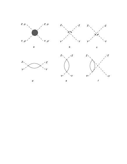
Figure 1: The scattering amplitude $ZY\rightarrow ZY$. Diagrams (b) and (c) contribute at tree level. The one-loop amplitude contains s-, t-, and u-channel diagram: (d), (e) and (f). Any of the fields $Z$, $Y$ and $\psi$ can propagate in the loop.

We now turn to the calculation of the S-matrix. Since all its components are related by symmetry, it suffices to calculate only one matrix element. We will compute the forward $ZY\rightarrow ZY$ scattering amplitude, drawn in fig. 1 (a). This particular amplitude is chosen because its calculation involves the least amount of combinatorics, which becomes rather cumbersome already at the one-loop level.

2.1 Tree-level amplitude

In two dimensions $2\rightarrow 2$ scattering has no phase space, and particles can either preserve or exchange their momenta, since the conservation condition of the two-momentum can be written as

$$\delta(p+p^{\prime}-k-k^{\prime})=\frac{p_{0}p^{\prime}_{0}}{p^{\prime}_{0}p_{1}-p_{0}p^{\prime}_{1}}\,\Bigl{(}\delta(p_{1}-k_{1})\delta(p_{1}-k^{\prime}_{1})+\delta(p_{1}-k^{\prime}_{1})\delta(p^{\prime}_{1}-k_{1})\Bigr{)}\;.$$ (2.4)

We consider the transition amplitude $Z(p)Y(p^{\prime})\rightarrow Z(p)Y(p^{\prime})$ which amounts in keeping only the first delta-function in the right-hand side. The Jacobian in (2.4) and relativistic normalization factors in the wave functions ($1/\sqrt{2p_{0}}$ for each external line) combine into an extra factor

$$\frac{1}{4}\,\frac{1}{p^{\prime}_{0}p_{1}-p_{0}p^{\prime}_{1}}=\frac{p_{-}p^{\prime}_{-}}{2m^{2}\left(p^{\prime}{}^{2}_{-}-p_{-}^{2}\right)}$$ (2.5)

that should be taken into account when extracting the S-matrix elements from Feynman diagrams. Here $p_{\pm}=(p_{0}\pm p_{1})/2$.

At tree level we need to evaluate just two diagrams, (b) and (c) in fig. 1. A simple calculation gives:

$$S=1-2i\gamma p_{-}p^{\prime}_{-}+\mathcal{O}(\gamma^{2})\;.$$ (2.6)

Upon identification (2.3), this agrees with the tree-level scattering amplitude in the sigma-model [15] in the limit

$$p_{-}\rightarrow\infty\quad,\quad p_{+}p_{-}=\mbox{fixed}\;.$$ (2.7)

2.2 One-loop amplitude

The one-loop diagrams are shown on fig. 1 (d), (e), (f). There are also several ways of distributing the derivatives in the vertices among various lines. The superficial degree of divergence of these diagrams is zero, which potentially leaves room for logarithmic UV divergences. Nevertheless, all the diagrams turn out to be finite. There are two reasons for that. First, fermi-bose cancelations reduce the degree of divergence by one and, second, the integrands behave as $k_{-}^{2}/k^{4}$ at large momenta, which gives zero upon angular integration even before the cancelations are taken into account.

Using Feynman rules that follow from the Lagrangian (2.2), we find for the one-loop amplitude (which has to be divided by the Jacobian (2.5) to get the S-matrix element):

$$\mathcal{A}_{\rm 1-loop} = 16\gamma^{2}\left(p_{-}^{2}+p^{\prime 2}_{-}\right)\left\{\int\frac{d^{2}k}{\left(2\pi\right)^{2}}\,\frac{\left(p_{-}+p^{\prime}_{-}\right)k_{-}}{\left(k^{2}-m^{2}\right)\left[\left(p+p^{\prime}-k\right)^{2}-m^{2}\right]}\right.$$ (2.8)

$$\qquad\qquad\qquad\;\;+\left.\int\frac{d^{2}k}{\left(2\pi\right)^{2}}\,\frac{\left(p_{-}-p^{\prime}_{-}\right)k_{-}}{\left(k^{2}-m^{2}\right)\left[\left(p-p^{\prime}-k\right)^{2}-m^{2}\right]}\right\}$$

$$+64\gamma^{2}p_{-}^{2}p^{\prime}{}^{2}_{-}\int\frac{d^{2}k}{\left(2\pi\right)^{2}}\,\frac{1}{\left(k^{2}-m^{2}\right)^{2}}\;.$$

The first two integrals correspond to the two-particle exchange in the s- and u-channels. The last term is the t-channel contribution. The s-channel amplitude contains an absorptive part from the on-shell intermediate states. This can be related to the tree amplitudes by unitarity (see below). The u-channel diagram is an analytic continuation of the s-channel contribution to Euclidean momenta. This happens to lead to additional cancelations, and the final result takes a relatively simple form:

$$S_{\rm 1-loop}=\frac{8i\gamma^{2}p_{-}^{3}p^{\prime}{}^{3}_{-}}{\pi\left(p^{\prime}{}^{2}_{-}-p_{-}^{2}\right)}\left(1-\frac{p^{\prime}{}^{2}_{-}+p_{-}^{2}}{p^{\prime}{}^{2}_{-}-p_{-}^{2}}\,\ln\frac{p^{\prime}_{-}}{p_{-}}\right)-\frac{2\gamma^{2}p_{-}^{2}p^{\prime}{}^{2}_{-}\left(p^{\prime}{}^{2}_{-}+p_{-}^{2}\right)}{\left(p^{\prime}_{-}-p_{-}\right)^{2}}\;.$$ (2.9)

3 Near-flat space limit of canonical S-matrix

In this section we compare our one-loop results to the $p_{-}\rightarrow\infty$ limit of the S-matrix of the full string sigma-model. The exact S-matrix is expressed in terms of the following kinemtical variables

$$x_{\pm}(p)=\frac{1+\sqrt{1+P^{2}}}{P}\,\,{\rm e}\,^{\pm\frac{i\pi p}{\sqrt{\lambda}}}\;,\qquad P=\frac{\sqrt{\lambda}}{\pi}\,\sin\frac{\pi p}{\sqrt{\lambda}}\;.$$ (3.1)

The amplitude for $ZY\rightarrow ZY$ scattering is given by [14, 16]

$$S^{\rm string}=\frac{1-\frac{1}{x^{\prime}_{+}x_{-}}}{1-\frac{1}{x^{\prime}_{-}x_{+}}}\,\,\frac{x^{\prime}_{-}-x_{+}}{x^{\prime}_{+}-x_{-}}\,\left(\frac{x^{\prime}_{-}-x_{-}}{x^{\prime}_{-}-x_{+}}\right)^{2}\,{\rm e}\,^{\frac{2i\pi p}{\sqrt{\lambda}}+i\theta(p,p^{\prime})}\;,$$ (3.2)

where $x_{\pm}\equiv x_{\pm}(p_{1})$, $x^{\prime}_{\pm}\equiv x_{\pm}(p^{\prime}_{1})$. The first term in the exponent indicates that we use the canonical S-matrix in the string basis [16] and the second term is the dressing phase discussed in the introduction. It is a gauge dependent quantity, however, in the near-flat-space limit all generalized light-cone gauges become identical. For simplicity we choose therefore the uniform gauge, where the dressing phase is of the form [6, 34]:

$$\theta(p,p^{\prime})=\frac{1}{\pi}\sum_{r,s=\pm}rs\,\chi(x_{r},x^{\prime}_{s})\;,$$ (3.3)

with (we will only need this second derivative)

$$\frac{\partial^{2}\chi(x,y)}{\partial x\,\partial y}=\frac{\sqrt{\lambda}}{2}\sum_{r=2}^{\infty}\sum_{n=0}^{\infty}\frac{c_{r,n}}{x^{r}y^{r+2n+1}}-\left(x\leftrightarrow y\right)\;,$$ (3.4)

and, to the one-loop accuracy [19],

$$c_{r,n}=\delta_{n\,0}-\frac{8}{\sqrt{\lambda}}\,\,\frac{(r-1)(r+2n)}{(2r+2n-1)(2n+1)}+\ldots\;.$$ (3.5)

We will now demonstrate that within the near-flat-space kinematics, the exact amplitude (3.2) agrees with (2.9) upon expansion in $\pi/\sqrt{\lambda}$ and identification (2.3). Let us first expand the phase $\theta(p,p^{\prime})$. Taking into account that the difference between $P$ in (3.1) and $p_{1}$ is unimportant at the one-loop level, we find from (3.3), (3.1):

$$\theta(p,p^{\prime})=-\frac{4\pi}{\lambda}\left(1+p_{0}\right)\left(1+p^{\prime}_{0}\right)\left.\frac{\partial^{2}\chi}{\partial x\,\partial y}\right|_{x=\frac{1+p_{0}}{p_{1}}\,,\,\,y=\frac{1+p^{\prime}_{0}}{p^{\prime}_{1}}}\;.$$ (3.6)

The summation in (3.4) yields

$$\frac{\partial^{2}\chi}{\partial x\,\partial y} = \frac{\sqrt{\lambda}}{2}\,\,\frac{x-y}{x^{2}y^{2}\left(xy-1\right)}$$ (3.7)

$$+\frac{2}{(xy-1)(x-y)}+\left[\frac{1}{(xy-1)^{2}}+\frac{1}{(x-y)^{2}}\right]\ln\frac{(x+1)(y-1)}{(x-1)(y+1)}+\ldots\;,$$

and we get

$$\theta(p,p^{\prime}) = \frac{\pi}{\sqrt{\lambda}}\,\,\frac{\left[(p^{\prime}_{0}-1)p_{1}-(p_{0}-1)p^{\prime}_{1}\right]^{2}}{p^{\prime}_{0}p_{1}-p_{0}p^{\prime}_{1}}+\frac{4\pi}{\lambda}\,\,\left(\frac{p_{1}p^{\prime}_{1}}{p^{\prime}_{0}p_{1}-p_{0}p^{\prime}_{1}}\right)^{2}\left[p^{\prime}_{0}p_{1}-p_{0}p^{\prime}_{1}\vphantom{\frac{(1+p_{0}+p_{1})(1+p^{\prime}_{0}-p^{\prime}_{1})}{(1+p_{0}-p_{1})(1+p^{\prime}_{0}+p^{\prime}_{1})}}\right.$$ (3.8)

$$\left.-p\cdot p^{\prime}\ln\frac{(1+p_{0}+p_{1})(1+p^{\prime}_{0}-p^{\prime}_{1})}{(1+p_{0}-p_{1})(1+p^{\prime}_{0}+p^{\prime}_{1})}\right]+\ldots\;.$$

The real part of the amplitude (the imaginary part of the S-matrix element) comes entirely from the dressing phase, and in the limit (2.7) becomes

$$\mathop{\mathrm{Im}}S^{\rm string}_{\rm 1-loop}=\frac{8\pi}{\lambda}\,\,\frac{p_{-}^{3}p^{\prime}{}^{3}_{-}}{p^{\prime}{}^{2}_{-}-p_{-}^{2}}\left(1-\frac{p^{\prime}{}^{2}_{-}+p_{-}^{2}}{p^{\prime}{}^{2}_{-}-p_{-}^{2}}\,\ln\frac{p^{\prime}_{-}}{p_{-}}\right)\;,$$ (3.9)

in complete agreement with (2.9).

The rest of (3.2), including the interference of the tree-level phases, determines the absorptive part of the amplitude:

$$\mathop{\mathrm{Re}}S^{\rm string}_{\rm 1-loop}=-\frac{\pi^{2}}{2\lambda}\left[(p^{\prime}_{0}p_{1}-p_{0}p^{\prime}_{1})^{2}+2(p_{1}^{2}-p_{1}p^{\prime}_{1}-p^{\prime}_{1}{}^{2})+\frac{(p_{1}+p^{\prime}_{1})^{2}(p_{1}^{2}+p^{\prime}_{1}{}^{2})}{(p^{\prime}_{0}p_{1}-p_{0}p^{\prime}_{1})^{2}}\right]\;.$$ (3.10)

In the limit (2.7) this becomes

$$\mathop{\mathrm{Re}}S^{\rm string}_{\rm 1-loop}=-\frac{2\pi^{2}}{\lambda}\,\frac{p_{-}^{2}p^{\prime}{}^{2}_{-}\left(p^{\prime}{}^{2}_{-}+p_{-}^{2}\right)}{\left(p^{\prime}_{-}-p_{-}\right)^{2}}\;,$$ (3.11)

also in agreement with (2.9).

The absorptive part of the one-loop amplitude can be reconstructed from tree-level amplitudes by unitarity. Writing

$$\mathbbm{S}=\mathbbm{1}+\frac{2\pi i}{\sqrt{\lambda}}\,T,$$

$$T\mathopen{|}Z_{\alpha\dot{\alpha}}Y^{\prime}_{a\dot{a}}\mathclose{\rangle}=2L(p,p^{\prime})\mathopen{|}Z_{\alpha\dot{\alpha}}Y^{\prime}_{a\dot{a}}\mathclose{\rangle}-H(p,p^{\prime})\mathopen{|}\mathnormal{\Psi}_{a\dot{\alpha}}\mathnormal{\Upsilon}^{\prime}_{\alpha\dot{a}}\mathclose{\rangle}+H(p,p^{\prime})\mathopen{|}\mathnormal{\Upsilon}_{\alpha\dot{a}}\mathnormal{\Psi}^{\prime}_{a\dot{\alpha}}\mathclose{\rangle}$$ (3.12)

and taking the tree-level amplitudes from [15]

$$L(p,p^{\prime}) =\frac{1}{4}\biggl{[}(1-2a)\left(p^{\prime}_{0}p_{1}-p_{0}p^{\prime}_{1}\right)+\frac{p_{1}^{2}-p^{\prime}_{1}{}^{2}}{p^{\prime}_{0}p_{1}-p_{0}p^{\prime}_{1}}\biggl{]}\;,$$ (3.13)

$$H(p,p^{\prime}) =\frac{1}{2}\,\frac{p_{1}p^{\prime}_{1}}{p^{\prime}_{0}p_{1}-p_{0}p^{\prime}_{1}}\,\frac{\left(p_{0}+1\right)\left(p^{\prime}_{0}+1\right)-p_{1}p^{\prime}_{1}}{\sqrt{\left(p_{0}+1\right)\left(p^{\prime}_{0}+1\right)}}\;,$$ (3.14)

we can use the optical theorem

$$\mathop{\mathrm{Im}}T=\frac{\pi}{\sqrt{\lambda}}\,T^{\dagger}T$$ (3.15)

to find the imaginary part of the one-loop contribution to $S^{\rm string}$. In the limit of large $p_{-}$ we find

$$\bigl{|}2L(p,p^{\prime})\bigr{|}^{2}+2\bigl{|}H(p,p^{\prime})\bigr{|}^{2}=\frac{p_{-}^{2}p^{\prime}{}^{2}_{-}\left(p^{\prime}_{-}{}^{2}+p_{-}^{2}\right)}{\left(p^{\prime}_{-}-p_{-}\right)^{2}}\;,$$ (3.16)

which, multiplied by $\frac{\pi}{\sqrt{\lambda}}\cdot\frac{2\pi}{\sqrt{\lambda}}$, is exactly what we have obtained before.

4 Conclusions and outlook

The string sigma-model on $AdS_{5}\times S^{5}$ simplifies considerably in the near-flat space limit thus making loop computations feasible. This opens up a possibility to check various conjectures about the exact S-matrix or the spectrum of the AdS string. It is not obvious that the reduced theory agrees with the full sigma-model at the quantum level, because low-momentum states could survive in loop diagrams even if the external legs all have large light-cone momenta. For instance, the momentum flowing through the t-channel loop in diagram fig. 1 (e) is zero. However, the agreement of the one-loop scattering amplitudes strongly suggests that the low-momentum states indeed decouple.

Another indication of the self-consistency of the near-flat space reduction is the finiteness of the one-loop amplitudes. The divergences cancel due to the asymmetric treatment of left- and right-moving modes. We believe that the same mechanism renders the model finite to all loop orders.

Acknowledgments

We would like to thank T. McLoughlin, R. Roiban and especially J. Minahan for interesting discussions. We would also like to thank J. Minahan for collaboration on the early stages of this project. The work of K.Z. was supported in part by the Swedish Research Council under contract 621-2004-3178, by grant NSh-8065.2006.2 for the support of scientific schools, and by RFBR grant 06-02-17383. The work of T.K. and K.Z. was supported by the Göran Gustafsson Foundation.

References

- [1] J. M. Maldacena, “The large N limit of superconformal field theories and supergravity”, Adv. Theor. Math. Phys. 2, 231 (1998), hep-th/9711200.
- [2] S. S. Gubser, I. R. Klebanov and A. M. Polyakov, “Gauge theory correlators from non-critical string theory”, Phys. Lett. B428, 105 (1998), hep-th/9802109.
- [3] E. Witten, “Anti-de Sitter space and holography”, Adv. Theor. Math. Phys. 2, 253 (1998), hep-th/9802150.
- [4] R. R. Metsaev and A. A. Tseytlin, “Type IIB superstring action in background”, Nucl. Phys. B533, 109 (1998), hep-th/9805028.
- [5] J. Maldacena and I. Swanson, “Connecting giant magnons to the pp-wave: An interpolating limit of ”, hep-th/0612079.
- [6] G. Arutyunov, S. Frolov and M. Staudacher, “Bethe ansatz for quantum strings”, JHEP 0410, 016 (2004), hep-th/0406256.
- [7] M. Staudacher, “The factorized S-matrix of CFT/AdS”, JHEP 0505, 054 (2005), hep-th/0412188.
- [8] J. A. Minahan and K. Zarembo, “The Bethe-ansatz for 4 super Yang-Mills”, JHEP 0303, 013 (2003), hep-th/0212208.
- [9] N. Beisert, C. Kristjansen and M. Staudacher, “The dilatation operator of 4 conformal super Yang-Mills theory”, Nucl. Phys. B664, 131 (2003), hep-th/0303060.
- [10] N. Beisert and M. Staudacher, “The 4 SYM Integrable Super Spin Chain”, Nucl. Phys. B670, 439 (2003), hep-th/0307042.
- [11] I. Bena, J. Polchinski and R. Roiban, “Hidden symmetries of the superstring”, Phys. Rev. D69, 046002 (2004), hep-th/0305116.
- [12] V. A. Kazakov, A. Marshakov, J. A. Minahan and K. Zarembo, “Classical/quantum integrability in AdS/CFT”, JHEP 0405, 024 (2004), hep-th/0402207.
- [13] N. Beisert and M. Staudacher, “Long-range Bethe ansaetze for gauge theory and strings”, Nucl. Phys. B727, 1 (2005), hep-th/0504190.
- [14] N. Beisert, “The dynamic S-matrix”, hep-th/0511082.
- [15] T. Klose, T. McLoughlin, R. Roiban and K. Zarembo, “Worldsheet scattering in ”, hep-th/0611169.
- [16] G. Arutyunov, S. Frolov and M. Zamaklar, “The Zamolodchikov-Faddeev algebra for superstring”, hep-th/0612229.
- [17] R. A. Janik, “The superstring worldsheet S-matrix and crossing symmetry”, Phys. Rev. D73, 086006 (2006), hep-th/0603038.
- [18] D. M. Hofman and J. M. Maldacena, “Giant magnons”, J. Phys. A39, 13095 (2006), hep-th/0604135.
- [19] R. Hernandez and E. Lopez, “Quantum corrections to the string Bethe ansatz”, JHEP 0607, 004 (2006), hep-th/0603204.
- [20] S. Frolov and A. A. Tseytlin, “Semiclassical quantization of rotating superstring in ”, JHEP 0206, 007 (2002), hep-th/0204226.
- [21] S. Frolov and A. A. Tseytlin, “Quantizing three-spin string solution in ”, JHEP 0307, 016 (2003), hep-th/0306130.
- [22] S. A. Frolov, I. Y. Park and A. A. Tseytlin, “On one-loop correction to energy of spinning strings in S(5)”, Phys. Rev. D71, 026006 (2005), hep-th/0408187.
- [23] I. Y. Park, A. Tirziu and A. A. Tseytlin, “Spinning strings in : One-loop correction to energy in SL(2) sector”, JHEP 0503, 013 (2005), hep-th/0501203.
- [24] S. Frolov, A. Tirziu and A. A. Tseytlin, “Logarithmic corrections to higher twist scaling at strong coupling from AdS/CFT”, hep-th/0611269.
- [25] S. Schafer-Nameki, M. Zamaklar and K. Zarembo, “Quantum corrections to spinning strings in and Bethe ansatz: A comparative study”, JHEP 0509, 051 (2005), hep-th/0507189.
- [26] N. Beisert and A. A. Tseytlin, “On quantum corrections to spinning strings and Bethe equations”, Phys. Lett. B629, 102 (2005), hep-th/0509084.
- [27] S. Schafer-Nameki and M. Zamaklar, “Stringy sums and corrections to the quantum string Bethe ansatz”, JHEP 0510, 044 (2005), hep-th/0509096.
- [28] S. Schafer-Nameki, “Exact expressions for quantum corrections to spinning strings”, Phys. Lett. B639, 571 (2006), hep-th/0602214.
- [29] L. Freyhult and C. Kristjansen, “A universality test of the quantum string Bethe ansatz”, Phys. Lett. B638, 258 (2006), hep-th/0604069.
- [30] S. Schafer-Nameki, M. Zamaklar and K. Zarembo, “How accurate is the quantum string Bethe ansatz?”, JHEP 0612, 020 (2006), hep-th/0610250.
- [31] M. K. Benna, S. Benvenuti, I. R. Klebanov and A. Scardicchio, “A test of the AdS/CFT correspondence using high-spin operators”, hep-th/0611135.
- [32] N. Beisert, R. Hernandez and E. Lopez, “A crossing-symmetric phase for strings”, JHEP 0611, 070 (2006), hep-th/0609044.
- [33] N. Beisert, B. Eden and M. Staudacher, “Transcendentality and crossing”, hep-th/0610251.
- [34] N. Beisert and T. Klose, “Long-range gl(n) integrable spin chains and plane-wave matrix theory”, J. Stat. Mech. 0607, P006 (2006), hep-th/0510124.