We discuss some aspects of higher-dimensional gravitational solitons and kinks, including in particular their stability. We illustrate our discussion with the examples of (non-BPS) higher-dimensional Taub-NUT solutions as the spatial metrics in $(6+1)$ and $(8+1)$ dimensions. We find them to be stable against small but non-infinitesimal disturbances, but unstable against large ones, which can lead to black-hole formation. In $(8+1)$ dimensions we find a continuous non-BPS family of asymptotically-conical solitons connecting a previously-known kink metric with the supersymmetric ${{{A}}_{8}}$ solution which has Spin(7) holonomy. All the solitonic spacetimes we consider are topologcally, but not geometrically, trivial. In an appendix we use the techniques developed in the paper to establish the linear stability of five-dimensional Myers-Perry black holes with equal angular momenta against cohomogeneity-2 perturbations.

1 Introduction

1.1 Gravitational solitons and kinks

By analogy with other areas of physics, a Gravitational Soliton in $n$ spacetime dimensions may be defined to be an everywhere complete non-singular globally stationary Lorentzian spacetime $M$, satisfying the vacuum Einstein equations [2]. Thus a gravitational soliton has by definition neither an event horizon nor an ergo-sphere and should therefore be distinguished from a stationary or static black hole, which is only required to be non-singular outside a a regular event horizon. For conventional solitons in flat space, one usually adds as a requirement that the solution not only be non-singular, but also have finite total energy. Furthermore, this energy is determined by the conserved charges the soliton may carry and also by quantities specifying asymptotic boundary conditions. Thus, for example, a magnetic monopole in Yang-Mills theory has a mass determined by its magnetic charge and by the vacuum expectation value of the Higgs field at infinity.

There are no gravitational solitons without horizons in four spacetime dimensions but in higher dimensons such objects do exist: perhaps the best known example being the Kaluza-Klein monopole in five dimensions [4, 14]. This has a metric of the form

$$d\hat{s}_{5}^{2}=-dt^{2}+ds_{4}^{2}\,,$$ (1)

where $ds_{4}^{2}$ is the self-dual Taub-NUT gravitational instanton metric. This four-dimensional metric is asymptotically locally flat, with a circle direction that stabilises to a constant length at large distance. The Kaluza-Klein monopole, upon reduction along this circle to $(3+1)$ spacetime dimensions, has a finite ADM mass given by the length of the circle at infinity.

1.2 Vacuum interpolation

In common with many flat-space solitons, the Kaluza-Klein monopole may be thought of as spatially interpolating between two inequivalent “vacua” or “ground states” of the theory, namely the flat five-dimensional Minkowski spacetime ${{E}}^{4,1}$ near the origin, and the compactified Kaluza-Klein ground state $S^{1}\times{{E}}^{3,1}$ near infinity. If a solitonic solution of the Einstein equations exhibits vacuum interpolation, it seems reasonable to refer to it also as a Gravitational Kink.

Again by analogy with other areas of physics, one does not expect to find an Asymptotically Flat gravitational soliton, i.e. one which outside a compact spatial set or world tube tends to the flat metric on $n$-dimensional Minkowski spacetime ${{E}}^{n-1,1}$. This is because it would interpolate between two copies of the same vacuum. Indeed, as we shall see shortly, this intuitive expectation is borne out by a No-Go theorem. Thus with respect to the flat Minkowski vacuum ${{E}}^{n-1,1}$, one cannot think of a gravitational soliton as having finite energy with respect to the flat Minkowski vacuum. Nevertheless, with respect to the ground state near infinity it may well have finite energy.

Vacuum interpolation also occurs in the case of extreme black holes or extreme black $p$-branes. Again, this is between different kinds of ground states; typically between a flat vacuum at infinity, and a compactified AdS${}_{p+2}\times K$, where $K$ is an $(n-p-2)$-dimensional compact manifold [10].

1.3 Classical stability

The definition given above does not specify whether a gravitational soliton should be stable. That is deliberate, because although to be important as a potentially long-lived classical “lump,” to use Coleman’s phrase [12], a gravitational soliton should at least be be classically stable against small but non-infinitesimal disturbances (i.e. not merely linearized fluctuations). It is not reasonable, however, to demand classical stability, in any gravitational theory, against all possible large disturbances, since nothing forbids gravitational collapse to a black hole with the same asymptotics. After all, even Minkowski spacetime is unstable against the possibility of a concentrated region of gravitational waves undergoing gravitational collapse to a black hole. Indeed in a recent numerical study of the dynamics of Kaluza-Klein monopoles [20], precisely such a collapse was seen to occur. The possibility of black hole formation, and the resulting spacetime singularities, invalidate the type of of topological stability criteria derived from cobordism theory that were discussed in [22].

Both Minkowski spacetime and the Kaluza-Klein monopole are supersymmetric, or BPS. Thus these two examples clearly demonstrate the fallacy of the widespread belief that to prove stability in general relativity it suffices to establish that the spacetime admits a Killing spinor.

The singularity theorems of classical general relativity show that these black holes contain spacetime singularities, which are a clear indication that the classical theory is incomplete. If these singularities are hidden inside event horizons, i.e. if cosmic censorship holds, they may not be an obstacle to studying the evolution of the exteriors of black holes. However, such black holes do not have a fixed mass, and may grow by, for example, absorbing radiation. Thus in general, black holes cannot be thought of as solitons. An exception may arise if one considers so-called extreme black holes, in which the mass may be determined entirely in terms of conserved charges [24]. We shall not discuss this type of “solitonic” black hole further in this paper.

1.4 Quantum stability

The stability considerations described above were purely classical. Quantum mechanically, black holes are unstable against thermal Hawking radiation. Thus in the case of the collapsed Kaluza-Klein monopole, it seems very likely that the ultimate quantum-mechanical state is the monopole itself, since the magnetic charge cannot be radiated away.

If, as is currently widely believed, the evaporation of neutral black holes leads to their complete disappearance, it would seem that Hawking evaporation is essential in order to solve the problem of classical singularities.

A frequently used criterion for the stability of a particle in quantum mechanics is that it has the least mass of any state carrying the same conserved charges. This criterion, often associated with BPS bounds, is often used to argue that various solitons, or indeed ground states, are stable. In the case of spacetimes, what is often in one’s mind is quantum tunnelling. While it is certainly true that a BPS condition, or the existence of a Killing spinor, may mean that tunnelling is impossible, it does not rule out the sort of classical instabilities we discussed previously.

1.5 Ultra-Staticity

The main subject of the present paper is the case of gravitational solitons in nine spacetime dimensions. This dimension is large enough to admit a rather richer structure of solitonic solutions than can be obtained in lower dimensions. Before describing our new results however, it may be useful to continue the general discussion, making it a little more precise. In particular we wish to establish the general result that that a gravitational soliton, as we have defined it, must be ultra-static, i.e. the (unwarped) product $M={{R}}\times\Sigma$ of time with a complete non-singular Ricci flat spatial Riemannian $(n-1)$-manifold $\Sigma$.

The assumption of global stationarity means that the spacetime is an ${{R}}$-bundle over $\Sigma$ the space of orbits of time translations. The metric may thus be cast in the form

$$ds^{2}=-V^{2}(dt+\omega_{i}dx^{i})^{2}+g_{ij}dx^{i}dx^{j}\,$$ (2)

where $i=1,2,\ldots,n-1$, and the everywhere non-vanishing strictly positive function $V$ and the Sagnac ${{R}}$-connection $\omega_{i}dx^{i}$ are independent of time. The curvature of the Sagnac connection is given by

$$F_{ij}=\partial_{i}\omega_{j}-\partial_{j}\omega_{i}\,.$$ (3)

We begin by noting that the vacuum Einstein equations imply that

$$\nabla_{i}\bigl{(}V^{3}F^{ij}\bigr{)}=0\,.$$ (4)

Multiplication by $\omega_{j}$ and integration by parts gives

$${\textstyle{\frac{\scriptstyle 1}{\scriptstyle 2}}}\int_{\Sigma}V^{3}F_{ij}F^{ij}\sqrt{g}d^{n-1}\,x=\int_{\infty}V^{3}\omega_{j}F^{ij}d\sigma_{i}.$$ (5)

If the boundary term at infinity vanishes, then we conclude that

$$F_{ij}=0\,.$$ (6)

The Einstein equations then imply

$$\nabla^{2}V=0\,.$$ (7)

Thus if $V$ is bounded at infinity, a standard argument based on the maximum principle shows that

$$V={\rm constant}$$ (8)

The remaining Einstein equation then implies that the spatial metric $g_{ij}$ is Ricci flat

$$R_{ij}=0.$$ (9)

If we assume that $\Sigma$ is simply connected, or pass to a finite covering space if it is not, we may set $\omega_{i}=0$, $V=1$ and the metric is ultra-static

$$ds^{2}=-dt^{2}+g_{ij}dx^{i}dx^{j}\,.$$ (10)

It follows from (10) that the question of the existence of gravitational solitons reduces completely to that of the existence of complete Ricci-flat spatial manifolds $\{\Sigma,g_{ij}\}$. It is known [18] that there are no non-trivial Asymptotically Euclidean metrics, and hence no asymptotically flat gravitational solitons but there are plenty of metrics which are Asymptotically Locally Euclidean as well as metrics with much more complicated asymptotics.

1.6 BPS solitons

Among the various possibilities for the Ricci-flat spatial metric, of particular interest are those admitting a covariantly constant spinor. They have reduced holomony, and if $n<12$, the spinor field is a Killing spinor of a supergravity theory and the solitons are thus supersymmetric. The existence of the Killing spinor allows one to relate the spectrum of the Lichnerowicz operator acting on symmetric traceless second-rank tensors to the spectrum of other differential operators. In this way, one may establish the linearized stability of solitons with special holonomy. For example, a metric with Spin(7) holonomy admits a covariantly constant self-dual 4-form. This 4-form may be used [40] to establish a 1-1 correspondence between the spectrum of the Lichnerowicz operator and the spectrum of the Hodge de-Rham operator acting on anti-self-dual 4-forms. Since the spectrum of the latter is manifestly non-negative, it follows that the Lichnerowicz operator has no modes of negative eigenvalue, and hence that Spin(7) solitons are stable at the linearised level. However, as we discussed earlier, they will not be stable against deformations sufficiently large that collapse to black holes takes place. Similar remarks about linearised stability apply to the other cases of special holonomy, which are as follows:

• Ricci-flat Kähler or Calabi-Yau with holonomy $SU(k)\subset SO(2k)$ and thus $n=2k+1$,

• Hyper-Kähler with holonomy $Sp(k)\subset SO(4k)$, and thus $n=4k+1$,

• Holonomy $G_{2}\subset SO(7)$, and thus $n=8$,

• Holonomy $Spin(7)\subset SO(8)$, and thus $n=9$.

Explicit complete non-singular metrics are known in all cases. The easiest examples to construct are cohomogenity one and are Asymptotically Conical(AC); they tend to Ricci flat cones over an Einstein manifolds which are:

• Holonomy $SU(k)\subset SO(2k)$: Einstein-Sasaki,

• Holonomy $Sp(k)\subset SO(4k)$: Einstein-Tri-Sasaski,

• Holonomy $G_{2}\subset SO(7)$ : Weak $SU(3)$,

• Holonomy $Spin(7)\subset SO(8)$: Weak $G_{2}$.

Other explicit cohomogenity one examples have been found which are Asymptotically Locally Conical (ALC). In this case a circle subgroup of the isometry group has orbits which tend to constant length at infinity. The ur-example is the Taub-NUT metric, i.e. the Kaluza-Klein monopole.

1.7 Cohomogeneity One and Cohmogeneity Two

In this paper we shall restrict attention to complete Ricci flat $(n-1)$-dimensional positive definite metrics which are of cohomogeneity one, that is whose isometry group $G$ has principal orbits which are $(n-2)$ dimensional. Such solutions give rise to static solitions on $n$-dimensional Lorentzian spacetime obtained by taking the metric product with time. The isometry group of the $n$-dimensional static spacetime is therefore the product ${{R}}\times G$.

We then construct a consistent time-dependent ansatz for the $n$-dimensional spacetime, which is is invariant under just the action of the orginal group $G$, and which agrees with the static soliton solution in the special case that there is no time dependence. The general time-dependent Lorentzian spacetime is thus of cohomogeneity two. The word “consistent” means that every solution of the resulting system of $(1+1)$-dimensional equations gives a solution of the $n$-dimensional vacuum Einstein equations.

The reason for restricting to cohomogeneity one and cohomogeneity two is not only for simplicity but because it allows us to exploit the considerable body of existing information in the literature on cohomogeneity-one Ricci-flat metrics.

We shall also mainly concentrate on the case when the spatial manifold is topologically, but not geometrically ${{R}}^{n}$.

2 Higher-Dimensional Time-Dependent Taub-NUT Solitons

One may consider a variety of higher-dimensional static metrics of the form $d\hat{s}^{2}=-dt^{2}+ds^{2}$, where $ds^{2}$ is a Ricci-flat spatial soliton metric. Then, following the same strategy as in [20], these metrics may be used to provide initial data for the time-dependent vacuum Einstein equations. Following the discussion in [20], we shall consider the higher-dimensional analogues [26, 28] of the four-dimensional self-dual Taub-NUT metric. It should be noted, however, that these higher-dimensional analogues are non-supersymmetric, in the sense that unlike the four-dimensional Taub-NUT case, there is no Killing spinor. We shall discuss the examples of the Taub-NUT metrics in six and eight dimensions below, after first presenting a general time-dependent ansatz.

2.1 The time-dependent ansatz

A suitably general time-dependent ansatz for our purposes is

$$d\hat{s}^{2}=-Ae^{-2\delta}\,dt^{2}+A^{-1}\,dr^{2}+r^{2}[e^{3B}\,d\Sigma_{m}^{2}+e^{-6mB}\,\sigma^{2}]\,,$$ (11)

where $d\Sigma_{m}^{2}$ is the metric on an Einstein-Kähler space of real dimension $2m$, normalized so that it satisfies $R_{ab}=2(m+1)g_{ab}$. The 1-form $\sigma$ is given by $\sigma=d\psi+{\cal B}$, where ${\cal B}$ is a potential on the Einstein-Kähler base space, such that $d{\cal B}=2J$, where $J$ is the Kähler form. The total dimension of the spacetime is $D=2m+3$.

Special cases of (11) include, if $e^{2\delta}=A$ and the metric is assumed to be independent of time, the Taub-NUT solitons. For these solutions, the Einstein-Kähler base spaces are taken to be ${{{C}}{{P}}}^{m}$. Other important special cases are the higher-dimensional Kerr and Kerr-AdS metrics. In the case of $(2m+3)$ dimensions, with all rotation parameters set equal, these have cohomogeneity one, and their stability can be analysed by a small extension of our procedure in which the Kaluza-Klein vector is retained also in the reduction. This is discussed in the Appendix.

The time-dependent Einstein equations $\hat{R}_{MN}=2(m+1)\lambda\,\hat{g}_{MN}$ for the metric (11) break up into momentum and Hamiltonian constraint equations

$$A^{\prime} = -\frac{2mA}{r}+\frac{2m}{(2m+1)r}\,[2(m+1)e^{-3B}-e^{-6(m+1)B}]-\frac{9}{2}mr(e^{2\delta}A^{-1}\,\dot{B}^{2}+A{B^{\prime}}^{2})$$

$$-\frac{c^{2}}{2(2m+1)}\,r^{-4m-3}\,e^{6mB}-2(m+1)\lambda\,r\,,$$

$$\dot{A} = -9mrA\dot{B}B^{\prime}\,,$$ (12)

a slicing condition

$$\delta^{\prime}=-\frac{9}{2}mr(e^{2\delta}\,A^{-2}\,\dot{B}^{2}+{B^{\prime}}^{2})\,,$$ (13)

and a wave equation

$$\Big{(}e^{\delta}\,A^{-1}\,r^{2m+1}\,\dot{B}\Big{)}^{.}-\Big{(}e^{-\delta}\,A\,r^{2m+1}\,B^{\prime}\Big{)}^{\prime}+\frac{4(m+1)}{3(2m+1)}e^{-\delta}\,r^{2m-1}\,(e^{-3B}-e^{-6(m+1)B})$$

$$+\frac{c^{2}}{2(2m+1)}r^{-2m-3}\,e^{-\delta}\,e^{6mB}=0\,.$$ (14)

If we define a mass functional $M(r,t)$, by writing $A=1-M(r,t)/r^{2m}-\lambda r^{2}$, then the Hamiltonian constraint becomes

$$M^{\prime} = \frac{9}{2}mr^{2m+1}\,(e^{2\delta}A^{-1}{\dot{B}}^{2}+A{B^{\prime}}^{2})+\frac{c^{2}}{2(2m+1)}r^{-2m-3}\,e^{6mB}$$ (15)

$$+\frac{2m}{2m+1}\,r^{2m-1}[(2m+1)+e^{-6(m+1)B}-2(m+1)e^{-3B}]\,.$$

Note that the right-hand side is manifestly positive.

In what follows, we shall specialise to the case of the vacuum Einstein equations, by setting $\lambda=0$.

2.2 The $(6+1)$-dimensional Taub-NUT soliton

The spatial metric of the time-independent $(6+1)$-dimensional Taub-NUT soliton is given by

$$ds_{6}^{2}=\frac{(\rho+\ell)^{2}\,d\rho^{2}}{2(\rho-\ell)(\rho+3\ell)}+\frac{2\ell^{2}(\rho-\ell)(\rho+3\ell)}{(\rho+\ell)^{2}}\,\sigma^{2}+(\rho^{2}-\ell^{2})\,d\Sigma_{2}^{2}\,,$$ (16)

with $\rho\geq\ell$, where the notation for $\sigma$ and $d\Sigma^{2}$ here is the same as in (11). One can see that the metric near $\rho=\ell$ approaches the origin of hyperspherical coordinates in ${{{R}}}^{6}$, by defining a new radial coordinate $y=\sqrt{2\ell(\rho-\ell)}$. At large $\rho$, the metric approaches ${{{R}}}^{5}$ times a circle of asymptotic radius $\sqrt{2}\,\ell$. The manifold on which (16) is defined has the topology of ${{{R}}}^{6}$.

Comparing with the ansatz (11), with $m=2$, we see that the six-dimensional Taub-NUT metric gives initial data with

$$e^{-15B_{0}}=\frac{2\ell^{2}(\rho+3\ell)}{(\rho+\ell)^{3}}\,,\qquad A_{0}=\frac{2(\rho+3\ell)(\rho-\ell)}{(\rho+\ell)^{2}}\,\Big{(}\frac{dr}{d\rho}\Big{)}^{2}\,,\qquad e^{2\delta_{0}}=A_{0}\,,$$ (17)

where

$$r^{10}=2\ell^{2}(\rho-\ell)^{5}(\rho+\ell)^{2}(\rho+3\ell)\,.$$ (18)

2.3 The $(8+1)$-dimensional Taub-NUT soliton

The spatial metric of the time-independent $(8+1)$-dimensional Taub-NUT soliton is given by

$$ds_{8}^{2}=\frac{5(\rho+\ell)^{3}\,d\rho^{2}}{8(\rho-\ell)(\rho^{2}+4\ell\rho+5\ell^{2})}+\frac{8\ell^{2}(\rho-\ell)(\rho^{2}+4\ell\rho+5\ell^{2})}{5(\rho+\ell)^{3}}\,\sigma^{2}+(\rho^{2}-\ell^{2})d\Sigma_{3}^{2}\,,$$ (19)

with $\rho\geq\ell$. It is defined on the manifold ${{{R}}}^{8}$.

Comparing with (11) with $m=3$, we see that the eight-dimensional Taub-NUT metric gives initial data with

$$e^{-21B_{0}}=\frac{8\ell^{2}(\rho^{2}+4\ell\rho+5\ell^{2})}{5(\rho+\ell)^{4}}\,,\qquad A_{0}=\frac{8(\rho-\ell)(\rho^{2}+4\ell\rho+5\ell^{2})}{5(\rho+\ell)^{3}}\,\Big{(}\frac{dr}{d\rho}\Big{)}^{2}\,,\qquad e^{2\delta_{0}}=A_{0}\,,$$ (20)

where

$$r^{14}={\textstyle{\frac{\scriptstyle 8}{\scriptstyle 5}}}\,\ell^{2}(\rho+\ell)^{3}(\rho-\ell)^{7}(\rho^{2}+4\ell\rho+5\ell^{2})\,.$$ (21)

As we shall see below this solution is a special case of a more general ansatz.

3 Nine-Dimensional Squashed Seven-Sphere Solitons

Our previous ansatz (11) was based on the Hopf fibring of $S^{2m+1}$ by $U(1)$ Hopf fibres over a ${{{C}}{{P}}}^{m}$ base manifold. In the case where $m=2p$, one can instead consider $S^{4p+3}$ regarded as an $SU(2)$ bundle over ${{{H}}{{P}}}^{p}$. The simplest case is for $p=1$, with $S^{7}$ regarded as an $SU(2)$ bundle over $S^{4}$. In this section, we shall consider a time-dependent ansatz for an $(8+1)$-dimensional time-dependent metric where the spatial 8-metric has surfaces at constant radius that have $S^{7}$ topology, fibred by $S^{3}$. Two deformation parameters will be included, one parameterising the volume of the $S^{3}$ fibres, and the other parameterising a homogeneous squashing of the $S^{3}$ fibres themselves.

We begin with some group-theoretic preliminaries, by considering left-invariant 1-forms $L_{AB}$ for $SO(5)$, These obey $L_{AB}=-L_{BA}$ and

$$dL_{AB}=L_{AC}\wedge L_{CB}\,.$$ (22)

We take the $SO(5)$ indices to range over $0\leq A\leq 4$, and split them as $A=(a,4)$, with $0\leq a\leq 3$. The $SO(4)$ 1-forms $L_{ab}$ are then expressed in an $SU(2)_{L}\times SU(2)_{R}$ basis with generators

$$R_{i}={\textstyle{\frac{\scriptstyle 1}{\scriptstyle 2}}}(L_{0i}+{\textstyle{\frac{\scriptstyle 1}{\scriptstyle 2}}}{\epsilon}_{ijk}L_{jk})\,,\qquad L_{i}={\textstyle{\frac{\scriptstyle 1}{\scriptstyle 2}}}(L_{0i}-{\textstyle{\frac{\scriptstyle 1}{\scriptstyle 2}}}{\epsilon}_{ijk}L_{jk})\,,$$ (23)

where $1\leq i\leq 3$. The $S^{7}=SO(5)/S0(3)$ coset is then spanned by the 1-forms

$$R_{i}\,,\qquad P_{a}\equiv{\textstyle{\frac{\scriptstyle 1}{\scriptstyle 2}}}L_{a4}\,.$$ (24)

(Note a rescaling of $P_{a}$, relative to [32]. This is done for convenience, to avoid factors of 2 later.) The algebra of the 1-forms is easily seen to be

$$dR_{i} = -{\epsilon}_{ijk}R_{j}\wedge R_{k}-J^{i}_{ab}\,P_{a}\wedge P_{b}\,,$$

$$dP_{a} = J^{i}_{ab}\,R_{i}\wedge P_{b}+\mathaccent 869{J}^{i}_{ab}\,L_{i}\wedge P_{b}\,,$$ (25)

$$dL_{i} = {\epsilon}_{ijk}L_{j}\wedge L_{k}-\mathaccent 869{J}^{i}_{ab}\,P_{a}\wedge P_{b}\,,$$

where we have defined antisymmetric self-dual and anti-self-dual ’tHooft tensors $J^{i}_{ab}$ and $\mathaccent 869{J}^{i}_{ab}$ by

$$J^{i}_{0j} = \delta^{i}_{j}\,,\qquad J^{i}_{jk}={\epsilon}_{ijk}\,,$$

$$\mathaccent 869{J}^{i}_{0j} = \delta^{i}_{j}\,,\qquad\mathaccent 869{J}^{i}_{jk}=-{\epsilon}_{ijk}\,.$$ (26)

The metric on the unit round $S^{7}$ is given by

$$d\Omega_{7}^{2}=R_{i}^{2}+P_{a}^{2}\,.$$ (27)

Our general time-dependent ansatz is

$$d\hat{s}_{9}^{2}=-A\,e^{-2\delta}\,dt^{2}+A^{-1}\,dr^{2}+r^{2}\,\Big{\{}e^{-4B}\,[e^{2C}\,(R_{1}^{2}+R_{2}^{2})+e^{-4C}\,R_{3}^{2}]+e^{3B}\,P_{a}^{2}\Big{\}}\,.$$ (28)

Straightforward calculations show that the Ricci-flatness of $d\hat{s}_{9}^{2}$ implies the following equations. First, we have the Hamiltonian and momentum constraints

$$A^{\prime} = -\frac{6}{r}A-\frac{6r}{7}A\Big{[}\frac{7}{2}({B^{\prime}}^{2}+e^{2\delta}\,A^{-2}\,{\dot{B}}^{2})+({C^{\prime}}^{2}+e^{2\delta}\,A^{-2}\,{\dot{C}}^{2})\Big{]}$$ (29)

$$+\frac{2}{7r}\,\Big{[}-e^{4B-8C}\!+\!4e^{4B-2C}\!-\!4e^{-10B+2C}\!-\!2e^{-10B-4C}\!+\!24e^{-3B}\Big{]}\,,$$

$$\dot{A} = -6r\,A(\dot{B}B^{\prime}+\frac{2}{7}\dot{C}C^{\prime})\,.$$ (30)

In addition, there is the slicing constraint

$$\delta^{\prime}=-3r\,\Big{[}({B^{\prime}}^{2}+e^{2\delta}\,A^{-2}\,{\dot{B}}^{2})+\frac{2}{7}({C^{\prime}}^{2}+e^{2\delta}\,A^{-2}\,{\dot{C}}^{2})\Big{]}\,.$$ (31)

Finally, we have the dynamical equations for the two squashing modes, which give

$$e^{\delta}(e^{\delta}\,A^{-1}\,r^{7}\dot{B})\dot{}-e^{\delta}(e^{-\delta}\,A\,r^{7}B^{\prime})^{\prime}$$

$$-\frac{4r^{5}}{21}\,(-e^{4B-8C}\!+\!4e^{4B-2C}\!+\!10e^{-10B+2C}\!+\!5e^{-10B-4C}\!-\!18e^{-3B})=0\,,$$ (32)

$$e^{\delta}(e^{\delta}\,A^{-1}\,r^{7}\dot{C})\dot{}-e^{\delta}(e^{-\delta}\,A\,r^{7}C^{\prime})^{\prime}$$

$$+\frac{4r^{5}}{3}\,(-e^{4B-8C}+e^{4B-2C}+e^{-10B+2C}-e^{-10B-4C})=0\,.$$ (33)

It can be straightforwardly verified that the constraints are indeed consistent with the dynamical equations of motion.

As a check, it can be verified that if we set $C={\textstyle{\frac{\scriptstyle 7}{\scriptstyle 2}}}B$, for which the ansatz (28) reduces to the special case of setting $m=3$ and ${\cal A}=0$ in (11), i.e. describing a squashing of $S^{7}$ viewed as a $U(1)$ bundle over ${{{C}}{{P}}}^{3}$, we indeed obtain the same equations as those given in section 2.1. Another check is instead to set $C=0$, in which case the system reduces to the one discussed in [34], where $S^{7}$ is viewed as a round $S^{3}$ bundle over $S^{4}$.

3.1 Static solutions

In this section we consider regular static asymptotically (locally) conical solutions of the system (29-33). Note that in agreement with Section 1.5 all static solutions are ultrastatic, i.e., $Ae^{-2\delta}=1$, thus equations (29-33) reduce to the following system of ordinary differential equations

$$e^{\delta}(e^{\delta}r^{7}B^{\prime})^{\prime}+\frac{4r^{5}}{21}\,(-e^{4B-8C}\!+\!4e^{4B-2C}\!+\!10e^{-10B+2C}\!+\!5e^{-10B-4C}\!-\!18e^{-3B})=0,$$ (34)

$$e^{\delta}(e^{\delta}r^{7}C^{\prime})^{\prime}-\frac{4r^{5}}{3}\,(-e^{4B-8C}+e^{4B-2C}+e^{-10B+2C}-e^{-10B-4C})=0\,.$$ (35)

$$\delta^{\prime}=-3r\,({B^{\prime}}^{2}+\frac{2}{7}{C^{\prime}}^{2})\,.$$ (36)

Regularity at the origin implies the following behavior for $r\rightarrow 0$

$$B\sim br^{2},\qquad C\sim cr^{2},\qquad e^{\delta}=1-(3b^{2}+\frac{6}{7}c^{2})r^{4}\,,$$ (37)

where $b$ and $c$ are free parameters. Using scaling symmetry, without loss of generality, we can set $b=1$. Then, (37) gives rise to a unique one-parameter family of local solutions parametrized by $c$. Numerical analysis shows that for any $c$ in the interval $0\leq c\leq 7/2$, these local solutions can be continued to infinity and thus give the desired global solutions (see Fig. 1). For the values of $c$ outside this interval the solutions become singular for a finite $r$. The asymptotic behavior of global solutions near infinity depends on $c$: for $0<c\leq 7/2$ the squashing modes grow logarithmically and $\delta$ goes to minus infinity, while for $c=0$ both $B$ and $\delta$ have finite limits. Thus unless $c=0$, the space sections are asymptotically locally conical, ALC, but in the limiting $c=0$ case they become asympototically conical (AC). For two values of $c$ the solutions are known is closed form: these are the Taub-NUT solution (19) which corresponds to $c=7/2$ and the so called ${{{A}}_{8}}$ solution [30, 32] which corresponds to $c=2$.

Below we discuss in detail the structure of static solutions and their stability properties.

Figure 1: Plot of $C/B$ for static solutions for several values of the shooting parameter $c$. For $0<c<7/2$ we have $C\sim(7/2)B-(1/2)\ln{2}$ for $r\rightarrow\infty$.

3.2 The Spin(7) background ${{{A}}_{8}}$ ($c=2$)

The ${{{A}}_{8}}$ solution is an ultra-static nine-dimensional vacuum solution whose space sections are asymptotically conical (AC).

$$ds_{9}^{2}=-dt^{2}+ds_{8}^{2}\,,$$ (38)

where $ds_{8}^{2}$ is a Ricci-flat metric with Spin(7) holonomy. A simple metric of this kind, which extends smoothly onto a manifold of ${{{R}}}^{8}$ topology, was obtained in [30, 32], where it was denoted by ${{{A}}_{8}}$. In the normalisation we are using here, it is given by

$$ds_{8}^{2}=\frac{(\rho+\ell)^{2}d\rho^{2}}{(\rho+3\ell)(\rho-\ell)}+(\rho+3\ell)(\rho-\ell)(R_{1}^{2}+R_{2}^{2})+\frac{4\ell^{2}(\rho+3\ell)(\rho-\ell)}{(\rho+\ell)^{2}}\,R_{3}^{2}+2(\rho^{2}-\ell^{2})P_{a}^{2}\,.$$ (39)

The radial coordinate $\rho$ lies in the range $\ell\leq\rho\leq\infty$. Near $\rho=\ell$ we may define a new radial coordinate $y=2\sqrt{(\rho-\ell)\ell}$, in terms of which the metric approaches

$$ds_{8}^{2}\sim dy^{2}+y^{2}(R_{i}^{2}+P_{a}^{2})$$ (40)

at small $y$. At large distance, $\rho\rightarrow\infty$, the metric approaches approaches ${{{R}}}^{7}$ times a circle of asymptotic radius $2\ell$. The situation is therefore closely analogous to that of the self-dual Taub-NUT metric in four dimensions.

Expressed in terms of the ansatz (28), the ${{{A}}_{8}}$ solution has the form

$$e^{21B} = \frac{2(\rho+\ell)^{5}}{\ell^{2}(\rho+3\ell)^{3}}\,,\qquad e^{-3C}=\frac{2\ell}{(\rho+\ell)}\,,$$

$$A = \frac{(\rho+3\ell)(\rho-\ell)}{(\rho+\ell)^{2}}\,\Big{(}\frac{dr}{d\rho}\Big{)}^{2}\,,\qquad e^{2\delta}=A\,,$$ (41)

where

$$r^{14}=64\ell^{2}(\rho+3\ell)^{3}(\rho-\ell)^{7}(\rho+\ell)^{2}\,.$$ (42)

3.3 The continuous family of solutions ($0<c\leq 7/2$)

We define the new independent variable $\tau$ by $re^{\delta}d/dr=d/d\tau$ and let $x=B$ and $y=\sqrt{\tfrac{2}{7}}\,C$. Then, assuming staticity, equations (34) and (35) take the form

$$\frac{d^{2}x}{d\tau^{2}}+6e^{\delta}\frac{dx}{d\tau}+\frac{\partial V}{\partial x}=0\,,\quad\frac{d^{2}y}{d\tau^{2}}+6e^{\delta}\frac{dy}{d\tau}+\frac{\partial V}{\partial y}=0\,,$$ (43)

where

$$V(x,y)=\frac{1}{21}\Big{(}-e^{4x-4\sqrt{14}y}+4e^{4x-\sqrt{14}y}-4e^{-10x+\sqrt{14}y}-2e^{-10x-2\sqrt{14}y}+24e^{-3x}\Big{)}\,,$$ (44)

and the slicing constraint (36) becomes

$$\frac{d}{d\tau}e^{\delta}=-3\left(\Big{(}\frac{dx}{d\tau}\Big{)}^{2}+\Big{(}\frac{dy}{d\tau}\Big{)}^{2}\right)\,.$$ (45)

The boundary conditions (37) translate to the following asymptotic behavior for $\tau\rightarrow-\infty$

$$x\sim b\,e^{2\tau},\quad y\sim\sqrt{\frac{2}{7}}c\,e^{2\tau},\quad e^{\delta}\sim 1-3(b^{2}+\frac{2}{7}c^{2})e^{4\tau}\,.$$ (46)

As above we set $b=1$, hence we have a one-parameter family of local solutions parametrized by $c$.

It is useful to interpret the above system in terms of the mechanical analogy of a sticky ball rolling on the surface $z=V(x,y)$. Due to the friction the energy of the ball,

$$E=\frac{1}{2}\Big{[}\Big{(}\frac{dx}{d\tau}\Big{)}^{2}+\Big{(}\frac{dy}{d\tau}\Big{)}^{2}\Big{]}+V(x,y)\,,$$ (47)

decreases in time

$$\frac{dE}{d\tau}=-6e^{\delta}\left(\Big{(}\frac{dx}{d\tau}\Big{)}^{2}+\Big{(}\frac{dy}{d\tau}\Big{)}^{2}\right)\leq 0\,.$$ (48)

Note that the combinations of equations (45) and (48) together with the boundary conditions (46) yield the constraint $E=e^{2\delta}$ which can be used to eliminate $e^{\delta}$ from equations (43).

Assuming that $x$ and $y$ are both positive and large we can solve the equations (43)-(45) asymptotically to get the following two possibilities

$$\text{(i)}\quad y\sim\sqrt{\frac{7}{2}}x\qquad\mbox{or}\qquad\text{(ii)}\quad y\sim\sqrt{\frac{7}{2}}x-\frac{\ln{2}}{\sqrt{14}}\,.$$ (49)

The case (i) is exceptional and corresponds to the ball rolling down the ridge, while the case (ii) is generic and it corresponds to the motion down the valley (on the left side of the valley there is the ridge which separates it from a cliff and on the right side there is a steep ascent). In the second case the asymptotic behavior of solutions for $\tau\rightarrow\infty$ is

$$x\sim\frac{2}{3}\ln{\tau}-\frac{1}{3}\ln\left(\frac{245}{10}\right),\qquad e^{\delta}\sim\frac{6}{\tau}\,.$$ (50)

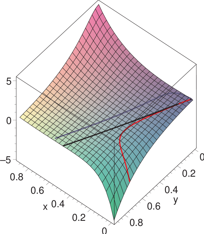
Figure 2: The potential $z=V(x,y)$ and three trajectories which start at the peak $(1,0,0)$ with different slopes (that is, different values of the parameter $c$). The black curve ($c=7/2$) represents the Taub-NUT solution, the dark blue curve ($c<7/2$) represents a generic solution of the continuous family, and the red curve shows a singular trajectory with $c>7/2$.

3.4 Stability of static solutions

The role of static solutions in dynamics depends on their stability properties. In this section we investigate the stability of static solutions presented above ($0<c\leq 7/2$).

3.4.1 Linear stability

Following the standard procedure we seek solutions in the form

$$B(t,r)=B_{0}(r)+B_{1}(t,r),\quad C(t,r)=C_{0}(r)+C_{1}(t,r),$$ (51)

$$A(t,r)=A_{0}(r)+A_{1}(t,r),\quad\delta(t,r)=\delta_{0}(r)+\delta_{1}(t,r)\,,$$ (52)

where the index $0$ denotes a static solution and the index $1$ denotes a perturbation. We substitute this expansion into equations (29)-(33) and linearize them. Integrating equation (30) we obtain

$$A_{1}=-6r\,A_{0}(B_{0}^{\prime}B_{1}+\frac{2}{7}C_{0}^{\prime}C_{1})\,,$$ (53)

and from equation (31) we get

$$\delta_{1}^{\prime}=-6r(B_{0}^{\prime}B_{1}^{\prime}+\frac{2}{7}C_{0}^{\prime}C_{1}^{\prime})\,.$$ (54)

Inserting equations (53) and (54) into the linearized equations (32) and (33) and separating the time dependence $B_{1}(t,r)=\exp(-i\lambda t)v_{\lambda}(r)$, $C_{1}(t,r)=\exp(-i\lambda t)u_{\lambda}(r)$ we get the eigenvalue equation for the spectrum of small perturbations

$$-\frac{1}{r^{7}}e^{\delta_{0}}\Big{(}e^{\delta_{0}}r^{7}\mathbf{S}_{\lambda}\Big{)}^{\prime}+\mathbf{K}\mathbf{S}_{\lambda}=\lambda^{2}\mathbf{S}_{\lambda}\,,$$ (55)

where

$$\mathbf{S}_{\lambda}=\begin{pmatrix}v_{\lambda}\\ u_{\lambda}\end{pmatrix}$$ (56)

and $\mathbf{K}$ is a $2\times 2$ matrix determined by the static solution. The matrix $\mathbf{K}$ is very complicated but fortunately we do not need it in an explicit form. To demonstrate stability we exploit the existence of the zero mode

$$\mathbf{S}_{0}=r\begin{pmatrix}B_{0}^{\prime}(r)\\ C_{0}^{\prime}(r)\end{pmatrix}\,,$$ (57)

which is due to the scaling invariance of the problem. From the above heuristic analysis of the behavior of static solutions it is clear (although not proved rigorously) that the functions $B_{0}(r)$ and $C_{0}(r)$ are monotone increasing, hence the components of the zero mode have no zeros. Thus, it follows from the Sturm-Liouville theory that there are no negative eigenvalues.

We point out that in the case of the ${{{A}}_{8}}$ manifold, the linearized stability of this solution follows from the existence of a covariantly-constant spinor in the Spin(7) holonomy manifold ${{{A}}_{8}}$, as discussed in section 1.6. Specifically, the spectrum of the Lichnerowicz operator describing transverse traceless metric perturbations is identical to the spectrum of the Hodge-de Rham operator acting on anti-self-dual 4-forms [40], and thus there can be no negative-eigenvalue modes and hence the solution is stable at the level of linearized perturbations.

3.4.2 Nonlinear stability

In order to verify numerically the nonlinear stability of static solutions numerically, we have expressed equations (29)-(33) in the first order form using the momentum variables

$$P_{B}=e^{\delta}A^{-1}\dot{B},\qquad P_{C}=e^{\delta}A^{-1}\dot{C}\,.$$ (58)

We have solved the resulting equation system using the free evolution scheme in which the function $A(t,r)$ is updated from the momentum constraint (30). Integration in time is done by the modified predictor-corrector McCormack method on a uniform spatial grid. The slicing constraint (31) is solved with the fourth order Runge-Kutta method. The whole procedure is second order accurate in time and fourth order in space. The results shown below were produced for initial data of the form

$$\!B(0,r)=B_{0}(r),\quad C(0,r)=C_{0}(r),\quad P_{B}(0,r)=p\left(\frac{r}{R}\right)^{4}e^{-\frac{(r-R)^{4}}{s^{4}}},\quad P_{C}(0,r)=0\,,$$ (59)

where the amplitude $p$ was varied and the parameters $R$ and $s$ were kept fixed. We have found that for small perturbations, that is for small values of the control parameter $p$, the solution returns to equilibrium and the excess energy of the perturbation is radiated away to infinity, while for large perturbations a black hole forms. The behavior is qualitatively the same for all static solutions (independently of $c$) and we illustrate it in Figs. 3 and 4 in the case of the ${{{A}}_{8}}$ solution.

Figure 3: Asymptotic stability of the solution ${{{A}}_{8}}$. For initial data (59) with a small amplitude ($p=0.1,R=3,s=1$) we plot a series of snapshots of the function $B(t,r)$ (where $t$ is central proper time). The dashed line shows the unperturbed ${{{A}}_{8}}$ solution.

Figure 4: Instability of the solution ${{{A}}_{8}}$ for large perturbations. For initial data (59) with a large amplitude ($p=0.3,R=3,s=1$) we plot a series of snapshots of the function $A(t,r)$ (where $t$ is central proper time). During the evolution $A(t,r)$ drops to zero at $r=r_{H}\approx 1.773$ which signals the formation of an apparent horizon there. Outside the horizon the solution relaxes to a static black hole.

3.5 The Eight-Dimensional Kink Solution ($c=0$)

In this section, we shall show the existence of a complete Ricci-flat 8-metric, which is asymptotically conical (AC), which we shall call the kink. It may be considered as spatially interpolating between flat Euclidean 8-space near the origin,

$$B=0,\quad C=0,\quad A=e^{2\delta}=1\,,$$ (60)

and the Ricci-flat cone over the Einstein-squashed 7-sphere at infinity,

$$B=\frac{\ln{5}}{7}\,,\quad C=0,\quad A=e^{2\delta}=9\cdot 5^{-10/7}\,.$$ (61)

It was demonstrated in [36], at the numerical level, that there exists a complete and non-singular metric that interpolates between these two constant solutions. It is defined on a manifold of ${{{R}}}^{8}$ topology. Here, we present a sketch of a proof of the existence of this kink solution.

Repeating the steps from Section 3.3 and setting $y=0$ in equations (43)-(45), we obtain the 3-dimensional autonomous system

$$\frac{d^{2}x}{d\tau^{2}}+6e^{\delta}\frac{dx}{d\tau}+\frac{\partial V}{\partial x}=0\,,$$ (62)

$$\frac{d}{d\tau}e^{\delta}=-3\Big{(}\frac{dx}{d\tau}\Big{)}^{2}\,,$$ (63)

where

$$V=\frac{1}{7}\Big{(}8e^{-3x}+e^{4x}-2e^{-10x}\Big{)}\,.$$ (64)

The boundary conditions (37) for $\tau\rightarrow-\infty$ simplify to

$$x\sim b\,e^{2\tau},\qquad e^{\delta}\sim 1-3b^{2}e^{4\tau}\,,$$ (65)

hence up to scaling given by $b$ we have a unique regular local solution.

As above, we can interpret this system in terms of the mechanical analogy of a ball rolling in the potential $V(x)$ with a variable friction (see Fig. 5).

Figure 5: In terms of the mechanical analogy the kink solution corresponds to the ball rolling down from the maximum of the potential $V=1$ at $x=0$ to the minimum $V=9\cdot 5^{-10/7}\approx 0.903$ at $x=\tfrac{\ln{5}}{7}$.

The energy of the ball

$$E=\frac{1}{2}\Big{(}\frac{dx}{d\tau}\Big{)}^{2}+V(x)$$ (66)

decreases in time because

$$\frac{dE}{d\tau}=-6e^{\delta}\Big{(}\frac{dx}{d\tau}\Big{)}^{2}\leq 0\,.$$ (67)

As in the general case we have the constraint $E=e^{2\delta}$. Using this constraint we eliminate $e^{\delta}$ from equation (62) and get the autonomous 2-dimensional dynamical system. This system has two critical points which correspond to the constant solutions (60) and (61): the saddle $(x=0,dx/d\tau=0)$ and the stable node $(x=\tfrac{\ln{5}}{7},dx/d\tau=0)$. The function $e^{2\delta}$ serves as the Lyapunov function, thus it is evident that the orbit starting from the saddle $(0,0)$ along the unstable manifold will end up at the stable node $(\tfrac{\ln{5}}{7},0)$ for $\tau\rightarrow\infty$. The linearization around this critical point yields the following asymptotic behavior for $\tau\rightarrow\infty$

$$\begin{pmatrix}x(\tau)-\frac{\ln{5}}{7}\\ dx/d\tau\end{pmatrix}=c_{1}e^{\lambda_{1}\tau}\mathbf{\xi}_{1}+c_{2}e^{\lambda_{2}\tau}\mathbf{\xi}_{2}\,,$$ (68)

where the eigenvalues are

$$\lambda_{1}=-\frac{8}{5}\cdot 5^{2/7},\qquad\lambda_{2}=-2\cdot 5^{2/7}\,,$$ (69)

and the corresponding eigenvectors are

$$\mathbf{\xi}_{1}=\begin{pmatrix}1\\ \lambda_{1}\end{pmatrix},\qquad\mathbf{\xi}_{2}=\begin{pmatrix}1\\ \lambda_{2}\end{pmatrix}\,.$$ (70)

The kink orbit approaches the node $(\tfrac{\ln{5}}{7},0)$ along the slow eigendirection $\mathbf{\xi}_{1}$. We claim that the kink orbit stays for all times in the first quadrant of the $(x,dx/d\tau)$ plane. To see this, consider an exceptional trajectory which approaches the node $(\tfrac{\ln{5}}{7},0)$ along the fast eigendirection $\mathbf{\xi}_{2}$ (that is, $c_{1}=0$ and $c_{2}<0$ in equation (68)). This trajectory, run backwards in time from the node, obviously cannot cross the line $x=\tfrac{\ln{5}}{7}$ and consequently it prevents the kink trajectory (which is trapped below the fast eigendirection trajectory) to do so. In terms of the mechanical analogue of a ball rolling in the potential $V$ the above analysis demonstrates that the motion of the ball is overdamped and moreover the ball rolling down from the maximum of the potential at $x=0$ cannot overshoot the minimum at $x=\tfrac{\ln{5}}{7}$.

Figure 6: The orbit of the kink. The node is approached along the slow eigendirection $\mathbf{\xi}_{1}$.

3.5.1 Analytic study of the kink solution

In this Section we describe an attempt to find the kink solution in the closed form. Although this attempt was not successful, we believe it is worth presenting because it yields a deeper analytic insight into the structure of equations. In addition, it provides an alternative way of proving the existence of the kink.

Consider the 8-metric

$$ds_{8}^{2}=dr^{2}+a^{2}(\sigma_{i}-A^{i})^{2}+b^{2}d\Omega_{4}^{2}\,,$$ (71)

where $d\Omega_{4}^{2}$ is the metric on the unit 4-sphere, $A^{i}$ is the 1-instanton solution on the $S^{4}$, and $\sigma_{i}$ are the left-invariant 1-forms of $SU(2)$. The flat metric on ${{{R}}}^{8}$ corresponds to $a=b={\textstyle{\frac{\scriptstyle 1}{\scriptstyle 2}}}r$, in which case the principal orbits are round 7-spheres for all values of $r$. In the kink solution, which is easily found by numerically solving the Ricci-flat equations for the metric ansatz (71), the metric approaches the flat form at small $r$, whilst as $r$ goes to infinity the principal orbits approach the squashed Einstein metric on $S^{7}$, for which $a^{2}/b^{2}=1/5$. In fact, as $r$ approaches infinity the metric functions have the limiting forms

$$a\longrightarrow\frac{3}{10}\,r\,,\qquad b\longrightarrow\frac{3}{2\sqrt{5}}\,r\,.$$ (72)

The nature of the numerical results can be seen in Figure 7 below:

      

Figure 7: The left-hand plot shows the functions $a$ (lower) and $b$ (upper) for the kink solution written using the metric ansatz (71). The right-hand plot shows $a^{2}/b^{2}$, which ranges from 1 (the round $S^{7}$) at small $r$ to $1/5$ (the squashed Einstein $S^{7}$) as $r$ goes to infinity.

One can also attempt to solve analytically for the kink solutions. (Note that, up to scaling, there is a unique such solution in each dimension $D=4n+4$.) Let us again consider the eight-dimensional case, and change variables so that (71) becomes

$$ds_{8}^{2}=\frac{e^{2\rho}\,d\rho^{2}}{h(\rho)}+e^{2\rho}\,f(\rho)\,(\sigma_{i}-A^{i})^{2}+e^{2\rho}\,d\Omega_{4}^{2}\,.$$ (73)

The specific choice of coordinate gauge in (73) is one that often allows one to obtain explicit solutions in terms of rational functions of $e^{\rho}$.

In the present case, we find that the metric is Ricci-flat if

$$h=\frac{(1+8f-2f^{2})f}{(8f^{2}+12f\dot{f}+{\dot{f}}^{2})}$$ (74)

and the function $f(\rho)$ satisfies the equation

$$2f(2f^{2}-8f-1)\ddot{f}+3(f-2){\dot{f}}^{3}+2(21f^{2}-34f+2){\dot{f}}^{2}$$

$$+12f(17f^{2}-26f+2)\dot{f}+56f^{2}(f-1)(5f-1)=0\,,$$ (75)

where a dot denotes a derivative with respect to $\rho$. This equation can be reduced to a single first-order differential equation as follows. We define $f(\rho)=x$ and $\dot{f}(\rho)=y(x)$, which implies

$$\rho=\int^{x}\frac{dz}{y(z)}\,,$$ (76)

and (75) becomes

$$y^{\prime}=\frac{3(x-2)y^{3}+2(2x^{2}-34x+2)y^{2}+12x(17x^{2}-26x+2)y+56x^{2}(x-1)(5x-1)}{2x(1+8x-2x^{2})y}\,,$$ (77)

where the prime denotes a derivative with respect to $x$. Note that $x$ is the squashing parameter, ranging from $x=1$ near the origin of the kink, where the 7-spheres are round, to $x=1/5$ in the asymptotic region near infinity, where the 7-spheres approach the squashed Einstein metric. The function $h$ appearing in the metric (73) is given by

$$h=\frac{x(1+8x-2x^{2})}{8x^{2}+12xy+y^{2}}\,.$$ (78)

The kink solution corresponds to $y(x)$ in (77) describing an arc, lying below the $y$ axis, starting at $(x,y)=(1/5,0)$ and ending at $(x,y)=(1,0)$. The asymptotic forms at the two endpoints of the arc are

$$y = -\frac{8}{15}(5x-1)-\frac{26}{105}(5x-1)^{2}+\frac{1954}{5145}(5x-1)^{3}+\cdots\,,$$

$$y = -2(1-x)+\frac{24}{7}(1-x)^{2}-\frac{640}{343}(1-x)^{3}+\cdots$$ (79)

respectively. In terms of the original variables, the kink solution runs from

$$f\sim 1\,,\qquad h\sim\frac{1}{4}$$ (80)

near the origin at $\rho=-\infty$ to

$$f\sim\frac{1}{5}\,,\qquad h\sim\frac{9}{20}$$ (81)

as $\rho$ approaches infinity.

It should be remarked that there exists a known solution to the equations, corresponding to the complete metric of Spin(7) holonomy found in [38, 40]. This corresponds to

$$f(\rho)=\frac{1}{5}(1-e^{-10\rho/3})\,,\qquad\hbox{or}\qquad y(x)=\frac{2}{3}(1-5x)\,.$$ (82)

This solution has the same behaviour at large $\rho$ (i.e. $x\rightarrow 1/5$) as we require for the kink solution, but it is very different at short distance (corresponding to $\rho=0$ in this parameterisation), since it has an $S^{4}$ bolt. In fact in the Spin(7) solution the variable $x$ lies in the range $0\leq x\leq 1/5$.

By making further transformations, one can cast (77) into a standard form for an Abel equation of the first kind. First, we make use of the known solution given in (82), and define a new dependent variable $v(x)$, related to $y(x)$ by

$$y(x)=\Big{(}\frac{2x^{2}-8x-1}{x^{2}(5x-1)v(x)}-\frac{3}{2(5x-1)}\Big{)}^{-1}\,.$$ (83)

After this change of variable, equation (77) becomes

$$x^{3}(5x-1)vv^{\prime}=x^{3}v^{2}+6x(4x^{2}+5x-1)v+28(1-x)(2x^{2}-8x-1)\,.$$ (84)

The further change of variable to $u(x)=(5x-1)^{-1/5}v(x)$ yields

$$x^{3}(5x-1)^{7/5}\,uu^{\prime}=6x(5x-1)^{1/5}(4x^{2}+5x-2)u+28(1-x)(2x^{2}-8x-1)\,.$$ (85)

It seems not to be possible to carry this further, since the change of independent variable required to put the equation into the canonical form $udu/dz-u=q(z)$ is given by taking

$$z=\frac{6(31x-2)}{x(5x-1)^{1/5}}-42\,\,5^{4/5}x^{-1/5}\,_{2}F_{1}({\textstyle{\frac{\scriptstyle 1}{\scriptstyle 5}}},{\textstyle{\frac{\scriptstyle 1}{\scriptstyle 5}}};{\textstyle{\frac{\scriptstyle 6}{\scriptstyle 5}}};{\textstyle{\frac{\scriptstyle 1}{\scriptstyle 5x}}})\,,$$ (86)

yielding

$$u\frac{du}{dz}-u=\frac{14(1-x)(2x^{2}-8x-1)}{3x(5x-1)^{1/5}(4x^{2}+5x-1)}\,.$$ (87)

Since one cannot invert (86) explicitly to obtain $x$ as a function of $u$, it appears that no further progress towards an analytic solution can be made.

Although attempts to solve (77) completely by analytic means have not proved successful, one can use this first-order system to perform a phase-plane analysis. This can be done by writing the first-order equation (77) in terms of an auxiliary parameter $t$, with

$$\frac{dx}{dt} = 2x(1+8x-2x^{2})y\,,$$

$$\frac{dy}{dt} = 3(x-2)y^{3}+2(2x^{2}-34x+2)y^{2}+12x(17x^{2}-26x+2)y$$ (88)

$$+56x^{2}(x-1)(5x-1)\,.$$

The kink solution lies within the region $1/5\leq x\leq 1$ in the phase plane. In fact it corresponds to the unique flow that starts at the saddle at $(x,y)=(1,0)$, and ends at the attractor at $(x,y)=(1/5,0)$. It is also instructive to look at the exact Spin(7) solution (82). This starts at the saddle at $(x,y)=(0,2/3)$, and flows (along a straight line) to the attractor at $(x,y)=(1/5,0)$. The kink solution, and the extrapolation of the exact Spin(7) solution into the region $1/5\leq x\leq 1$, are shown in Figure 8 below.

      

Figure 8: The numerical solutions of (77) corresponding, in the left-hand plot, to the exact solution of Spin(7) holonomy given in (82) (extrapolated into the region $1/5\leq x\leq 1$ depicted here), and in the right-hand diagram, to the kink solution. The latter corresponds to a trajectory from the saddle at $x=1$, $y=0$ to the attractor at $x=1/5$, $y=0$.

3.5.2 Stability of the kink soliton

In the case of the kink the eigenvalue problem (55) for the spectrum of small perturbations around a static solution reduces to the single equation

$$-\frac{1}{r^{7}}e^{\delta_{0}}\Big{(}e^{\delta_{0}}r^{7}v^{\prime}_{\lambda}\Big{)}^{\prime}+Kv_{\lambda}=\lambda^{2}v_{\lambda}\,,$$ (89)

where

$$K = \frac{1}{7r^{2}}\Big{(}-72e^{-3B_{0}}-16e^{4B_{0}}+200e^{-200B_{0}}\Big{)}$$

$$+ \frac{1}{7r}\Big{(}288e^{-3B_{0}}-48e^{4B_{0}}-240e^{-200B_{0}}\Big{)}B^{\prime}_{0}$$

$$+ \frac{1}{7}\Big{(}-288e^{-3B_{0}}-36e^{4B_{0}}+72e^{-200B_{0}}\Big{)}{B^{\prime}_{0}}^{2}\,.$$

We have shown above that the profile function of the kink is monotone, hence the zero mode corresponding to the scaling freedom, $v_{0}=rB_{0}^{\prime}(r)$, has no zeros which implies by the standard Sturm-Liouville theory there are no negative eigenvalues. Thus, the kink solution is linearly stable within our ansatz.

The behavior of the kink under non-infinitesimal perturbations was studied numerically by the methods described in Section 3.4.2. As in the case of other static solutions we found that for small perturbations the kink is asymptotically stable, while for large perturbations it collapses to a black hole. The numerical evidence for these properties is shown in Figs. 9 and 10.

(a)

(b)

Figure 9: Asymptotic stability of the kink solution. For small perturbations of the kink we plot a series of snapshots of (a) the function $B(t,r)$ and (b) the function $A(t,r)$. The dashed line shows the unperturbed kink solution.

(a)

(b)

Figure 10: Instability of the kink for large perturbations. For large perturbations of the kink we plot a series of snapshots of (a) the function $B(t,r)$ and (b) the function $A(t,r)$. During the evolution $A(t,r)$ drops to zero at $r=r_{H}\approx 1.754$ which signals the formation of an apparent horizon there. Outside the horizon the solution relaxes to a static black hole.

4 Conclusions

In this paper, we have studied gravitational solitons and kinks in higher dimensions. Our focus has been the study of their stability, principally in the case of solitons in nine dimensions. We have considered various possibilities for the spatial metric, including examples such as the higher-dimensional Taub-NUT metrics [26, 28], which are not supersymmetric, and also the example of the ${{{A}}_{8}}$ 8-metric of Spin(7) holonomy [30, 32], which is supersymmetric. All the solitons we consider are trivial topologically (i.e. ${{{R}}}^{n}$ topology), but non-trivial geometrically. We studied the question of stability first at the linearised level, using analyic methods, and found that in all cases the solitons are linearly stable. Numerical analysis indicates that this stability persists for non-infinitesimal perturbations also, provided they are small enough in magnitude. The numerical analysis also shows that for sufficiently large perturbations the solitons are all unstable to black-hole formation. This is not altogether surprising, since even flat Minkowski spacetime is unstable to sufficiently large perturbations, which can lead to the formation of a black hole. These instabilities provide a salutory reminder of the fact that in gravitational theories supersymmetry is not a guarantor of stability beyond the linearised level.

We also studied in detail a kink metric in eight dimensions, whose existence was first encountered in [36]. It is a non-trivial cohomogeneity-1 metric on ${{{R}}}^{8}$, in the which the level sets are homogeneous 7-spheres viewed as $S^{3}$ bundles over $S^{4}$. At small distances the level surfaces approach the round 7-sphere and the metric is of the form near the origin of Euclidean 8-space. At large distances the level surfaces approach the squashed $S^{7}$ Einstein metric in the family of $S^{3}$ bundles over $S^{4}$. We showed that the Ricci-flatness conditions for the kink metric can be reduced to a first-order Abel equation of the first kind, but it appears not to be possible to obtain an explicit solution analytically. Our discussion includes a proof of the existence of the Ricci-flat metric.

Acknowledgments.

The research of PB and TC was supported in part by the Polish Research Committee grant 1PO3B01229. The research of C.N.P. is supported in part by DOE grant DE-FG03-95ER40917.

Appendix A Nine-Dimensional Schwarzschild

This section contains a brief summary of the analysis of the stability of the nine-dimensional Schwarzschild solution within the framework of the deformations considered in this paper.

If we expand around the nine-dimensional Schwarzschild background, for which

$$A_{0}=1-\frac{2m}{r^{6}}\,,\qquad\delta_{0}=0\,,\qquad\phi_{1}^{(0)}=0\,,\qquad\phi_{2}^{(0)}=0\,,$$ (91)

we find that working to first order in fluctuations we can keep $A=A_{0}$ and $\delta=0$. For the dynamical fields, we shall now use $\phi_{1}$ and $\phi_{2}$ to denote the linearised fluctuations. Introducing the “tortoise coordinate” $x$ via $dx/dr=A_{0}^{-1}$, and defining

$$\phi_{1}=r^{-7/2}\,u_{1}\,,\qquad\phi_{2}=r^{-7/2}\,u_{2}\,,$$ (92)

we find that these satisfy

$$\ddot{u}_{1}-\frac{\partial^{2}u_{1}}{\partial x^{2}}+V\,u_{1}=0\,,\qquad\ddot{u}_{2}-\frac{\partial^{2}u_{2}}{\partial x^{2}}+V\,u_{2}=0\,,$$ (93)

where the potential $V$ (which is the same for both $u_{1}$ and $u_{2}$) is given by

$$V=-{\textstyle{\frac{\scriptstyle 1}{\scriptstyle 4}}}\Big{(}1-\frac{2m}{r^{6}}\Big{)}\Big{(}\frac{99}{r^{2}}+\frac{98m}{r^{8}}\Big{)}\,.$$ (94)

Note that this is the same potential as was encountered in [34] in the analysis of the nine-dimensional perturbations of Schwarzschild with a single dynamical variable (corresponding to $u_{2}=0$ here.)

Appendix B Time Evolution of Kerr-AdS Black Holes

In this appendix, we use the techniques of this paper to analyse the stability of a particular class of five-dimensional rotating black holes. The general methods extend extend to any black hole having all angular momenta equal, but in this appendix we restrict attention to the $(4+1)$-dimensional case. This means that we can again consider an ansatz with $SU(2)\times U(1)$ isometry on the constant-radius spatial sections.

The five-dimensional Kerr-AdS solution [42] with equal angular momenta is given by

$$ds_{5}^{2}=-\frac{Gdt^{2}}{\Big{(}1+\frac{2Ma^{2}}{\rho^{4}}\Big{)}}+\frac{d\rho^{2}}{G}+{\textstyle{\frac{\scriptstyle 1}{\scriptstyle 4}}}\rho^{2}\Big{(}1+\frac{2Ma^{2}}{\rho^{4}}\Big{)}(\sigma_{3}+2\Omega\,dt)^{2}+{\textstyle{\frac{\scriptstyle 1}{\scriptstyle 4}}}\rho^{2}\,(\sigma_{1}^{2}+\sigma_{2}^{2})\,,$$ (95)

where

$$G = \Big{(}1-\lambda\,\rho^{2}-\frac{2M\,\Xi}{\rho^{2}}+\frac{2Ma^{2}}{\rho^{4}}\Big{)}\,,$$

$$\Omega = \frac{2Ma}{\rho^{4}+2Ma^{2}}\,,\qquad\Xi=1+\lambda a^{2}\,.$$ (96)

The metric satisfies $R_{MN}=4\lambda g_{MN}$. Thus for the asymptotically AdS case we require $\lambda<0$.

The new feature in our analysis is the inclusion of the Kaluza-Klein vector in the dimensional reduction. The electric charge associated with this field is proportional to the angular momentum of the black hole. Thus we make the following reduction ansatz

$$d\hat{s}^{2}=e^{2\alpha\,\varphi}\,ds^{2}+e^{2\beta\,\varphi}\,\Big{[}e^{4\gamma\,\phi}\,(\sigma_{3}+{\cal A})^{2}+e^{-2\gamma\,\phi}\,(\sigma_{1}^{2}+\sigma_{2}^{2})\Big{]}\,.$$ (97)

For the time being, we consider the base metric $ds^{2}$ to have dimension $n$. Later, we shall specialise to the case of immediate interest, namely $n=2$. We choose the natural vielbein basis

$$\hat{e}^{0} = e^{\beta\varphi+2\gamma\phi}\,(\sigma_{3}+{\cal A})\,,$$

$$\hat{e}^{\alpha} = e^{\alpha\varphi}\,e^{\alpha}\,,$$

$$\hat{e}^{a} = e^{\beta\varphi-\gamma\phi}\,\sigma_{a}\,,\qquad a=1,2\,.$$ (98)

After some calculation, we arrive at the following non-vanishing Ricci-tensor components (in the vielbein basis):

$$\hat{R}_{00} = e^{-2\alpha\varphi}\,\Big{\{}-(3\beta+(n-2)\alpha)[\beta(\nabla\varphi)^{2}+2\gamma\nabla\varphi\cdot\nabla\phi]-\beta\mathord{{\vbox{\hrule height=0.7pt\hbox{\vrule width=0.7pt,height=6.8pt\kern 6.8pt\vrule width=0.7pt} \hrule height=0.7pt}}\hbox{\hskip 1.0pt}}\varphi-2\gamma\mathord{{\vbox{\hrule height=0.7pt\hbox{\vrule width=0.7pt,height=6.8pt\kern 6.8pt\vrule width=0.7pt} \hrule height=0.7pt}}\hbox{\hskip 1.0pt}}\phi\Big{\}}$$

$$+{\textstyle{\frac{\scriptstyle 1}{\scriptstyle 4}}}e^{(2\beta-4\alpha)\varphi+4\gamma\phi}\,{\cal F}^{2}+{\textstyle{\frac{\scriptstyle 1}{\scriptstyle 2}}}e^{-2\beta\varphi+8\gamma\phi}\,,$$

$$\hat{R}_{\alpha\beta} = e^{-2\alpha\varphi}\,\Big{\{}(6\alpha\beta-3\beta^{2}+(n-2)\alpha^{2})\nabla_{\alpha}\varphi\,\nabla_{\beta}\varphi-6\gamma^{2}\nabla_{\alpha}\phi\,\nabla_{\beta}\phi-(3\beta+(n-2)\alpha)\nabla_{\alpha}\nabla_{\beta}\varphi\Big{\}}$$

$$-\alpha e^{-2\alpha\varphi}\,\Big{\{}(3\beta+(n-2)\alpha)(\nabla\varphi)^{2}+\mathord{{\vbox{\hrule height=0.7pt\hbox{\vrule width=0.7pt,height=6.8pt\kern 6.8pt\vrule width=0.7pt} \hrule height=0.7pt}}\hbox{\hskip 1.0pt}}\varphi\Big{\}}\eta_{\alpha\beta}-{\textstyle{\frac{\scriptstyle 1}{\scriptstyle 2}}}e^{(2\beta-4\alpha)\varphi+4\gamma\phi}\,{\cal F}_{\alpha\gamma}\,{\cal F}_{\beta}{}^{\gamma}+e^{-2\alpha\varphi}\,R_{\alpha\beta}\,,$$

$$\hat{R}_{ab} = \Big{[}e^{-2\alpha\varphi}\,\Big{\{}(3\beta+(n-2)\alpha)[\gamma\nabla\varphi\cdot\nabla\phi-\beta(\nabla\varphi)^{2}]+\gamma\mathord{{\vbox{\hrule height=0.7pt\hbox{\vrule width=0.7pt,height=6.8pt\kern 6.8pt\vrule width=0.7pt} \hrule height=0.7pt}}\hbox{\hskip 1.0pt}}\phi-\beta\mathord{{\vbox{\hrule height=0.7pt\hbox{\vrule width=0.7pt,height=6.8pt\kern 6.8pt\vrule width=0.7pt} \hrule height=0.7pt}}\hbox{\hskip 1.0pt}}\varphi\Big{\}}$$

$$\qquad-{\textstyle{\frac{\scriptstyle 1}{\scriptstyle 2}}}e^{-2\beta\varphi+2\gamma\phi}\,(e^{6\gamma\phi}-2)\Big{]}\,\delta_{ab}\,,$$

$$\hat{R}_{0\alpha} = {\textstyle{\frac{\scriptstyle 1}{\scriptstyle 2}}}e^{(\alpha-\beta)\varphi-2\gamma\phi}\,\nabla_{\beta}\Big{(}e^{(2\beta-4\alpha)\varphi+4\gamma\phi}\,{\cal F}_{\alpha}{}^{\beta}\Big{)}+{\textstyle{\frac{\scriptstyle 1}{\scriptstyle 2}}}(n\alpha+3\beta)\,e^{(\beta-3\alpha)\varphi+2\gamma\phi}\,{\cal F}_{\alpha}{}^{\beta}\,\nabla_{\beta}\varphi\,,$$ (99)

where ${\cal F}=d{\cal A}$.

Specialising to the case $n=2$, these expressions give

$$\hat{R}_{00} = e^{-2\alpha\varphi}\,\Big{\{}-3\beta[\beta(\nabla\varphi)^{2}+2\gamma\nabla\varphi\cdot\nabla\phi]-\beta\mathord{{\vbox{\hrule height=0.7pt\hbox{\vrule width=0.7pt,height=6.8pt\kern 6.8pt\vrule width=0.7pt} \hrule height=0.7pt}}\hbox{\hskip 1.0pt}}\varphi-2\gamma\mathord{{\vbox{\hrule height=0.7pt\hbox{\vrule width=0.7pt,height=6.8pt\kern 6.8pt\vrule width=0.7pt} \hrule height=0.7pt}}\hbox{\hskip 1.0pt}}\phi\Big{\}}$$ (100)

$$+{\textstyle{\frac{\scriptstyle 1}{\scriptstyle 4}}}e^{(2\beta-4\alpha)\varphi+4\gamma\phi}\,{\cal F}^{2}+{\textstyle{\frac{\scriptstyle 1}{\scriptstyle 2}}}e^{-2\beta\varphi+8\gamma\phi}\,,$$

$$\hat{R}_{\alpha\beta} = e^{-2\alpha\varphi}\,\Big{\{}3\beta(2\alpha-\beta)\nabla_{\alpha}\varphi\,\nabla_{\beta}\varphi-6\gamma^{2}\nabla_{\alpha}\phi\,\nabla_{\beta}\phi-3\beta\nabla_{\alpha}\nabla_{\beta}\varphi\Big{\}}$$ (101)

$$-\alpha e^{-2\alpha\varphi}\,\Big{\{}3\beta(\nabla\varphi)^{2}+\mathord{{\vbox{\hrule height=0.7pt\hbox{\vrule width=0.7pt,height=6.8pt\kern 6.8pt\vrule width=0.7pt} \hrule height=0.7pt}}\hbox{\hskip 1.0pt}}\varphi\Big{\}}\eta_{\alpha\beta}-{\textstyle{\frac{\scriptstyle 1}{\scriptstyle 2}}}e^{(2\beta-4\alpha)\varphi+4\gamma\phi}\,{\cal F}_{\alpha\gamma}\,{\cal F}_{\beta}{}^{\gamma}+e^{-2\alpha\varphi}\,R_{\alpha\beta}\,,$$

$$\hat{R}_{ab} = \Big{[}e^{-2\alpha\varphi}\,\Big{\{}3\beta[\gamma\nabla\varphi\cdot\nabla\phi-\beta(\nabla\varphi)^{2}]+\gamma\mathord{{\vbox{\hrule height=0.7pt\hbox{\vrule width=0.7pt,height=6.8pt\kern 6.8pt\vrule width=0.7pt} \hrule height=0.7pt}}\hbox{\hskip 1.0pt}}\phi-\beta\mathord{{\vbox{\hrule height=0.7pt\hbox{\vrule width=0.7pt,height=6.8pt\kern 6.8pt\vrule width=0.7pt} \hrule height=0.7pt}}\hbox{\hskip 1.0pt}}\varphi\Big{\}}-{\textstyle{\frac{\scriptstyle 1}{\scriptstyle 2}}}e^{-2\beta\varphi+2\gamma\phi}\,(e^{6\gamma\phi}-2)\Big{]}\,\delta_{ab}\,,$$ (102)

$$\hat{R}_{0\alpha} = {\textstyle{\frac{\scriptstyle 1}{\scriptstyle 2}}}e^{-(\alpha+4\beta)\varphi-2\gamma\phi}\,\nabla_{\beta}\Big{(}e^{(5\beta-2\alpha)\varphi+4\gamma\phi}\,{\cal F}_{\alpha}{}^{\beta}\Big{)}\,.$$ (103)

Following the analysis in [16], we use the volume of the $S^{3}$ to parameterise the radial direction, and write

$$d\hat{s}^{2}=-Ae^{-2\delta}\,dt^{2}+A^{-1}\,dr^{2}+{\textstyle{\frac{\scriptstyle 1}{\scriptstyle 4}}}r^{2}[e^{2B}(\sigma_{1}^{2}+\sigma_{2}^{2})+e^{-4B}\,(\sigma_{3}+{\cal A})^{2}]\,.$$ (104)

Thus, comparing with (97), we have

$$e^{\beta\varphi}={\textstyle{\frac{\scriptstyle 1}{\scriptstyle 2}}}r\,,\qquad\gamma\phi=-B\,,\qquad ds^{2}=e^{-2\alpha\varphi}\,(-Ae^{-2\delta}\,dt^{2}+A^{-1}\,dr^{2})\,.$$ (105)

Substituting into the Einstein equation

$$\hat{R}_{MN}=4\lambda\,\hat{g}_{MN}\,,$$ (106)

we note from (103) that

$${\cal F}_{\mu\nu}=c\,{\epsilon}_{\mu\nu}\,e^{(2\alpha-5\beta)\varphi-4\gamma\phi}\,,$$ (107)

where $c$ is a constant and ${\epsilon}_{\mu\nu}$ is the Levi-Civita tensor in the metric $ds^{2}$. This expression can be substituted into the remaining Einstein equations, leading to the momentum and Hamiltonian constraints

$$A^{\prime} = -\frac{2A}{r}+\frac{1}{3r}\,(8e^{-2B}-2e^{-8B})-2r(e^{2\delta}A^{-1}\,\dot{B}^{2}+A{B^{\prime}}^{2})-\frac{128c^{2}}{3r^{7}}\,e^{4B}-4\lambda\,r\,,$$

$$\dot{A} = -4rA\dot{B}B^{\prime}\,,$$ (108)

the slicing condition

$$\delta^{\prime}=-2r(e^{2\delta}\,A^{-2}\,\dot{B}^{2}+{B^{\prime}}^{2})\,,$$ (109)

and the wave equation

$$\Big{(}e^{\delta}\,A^{-1}\,r^{3}\,\dot{B}\Big{)}^{.}-\Big{(}e^{-\delta}\,A\,r^{3}\,B^{\prime}\Big{)}^{\prime}+{\textstyle{\frac{\scriptstyle 4}{\scriptstyle 3}}}e^{-\delta}\,r\,(e^{-2B}-e^{-8B})+\frac{128c^{2}}{3r^{5}}\,e^{-\delta}\,e^{4B}=0\,.$$ (110)

It is straightforward to verify the self consistency of the equations. Namely, that the vanishing of the dot of $A^{\prime}$ minus the prime of $\dot{A}$ in (108) yields, after using (109) and (108), the wave equation (110) for $B$.

Defining $A=1-m(r,t)/r^{2}-\lambda r^{2}$, the Hamiltonian constraint in (108) becomes

$$m^{\prime}=2r^{3}(e^{2\delta}\,A^{-1}\,\dot{B}^{2}+A{B^{\prime}}^{2})+{\textstyle{\frac{\scriptstyle 2}{\scriptstyle 3}}}r(3+e^{-8B}-4e^{-2B})+\frac{128c^{2}}{3r^{5}}\,e^{4B}\,.$$ (111)

This is manifestly positive.

Note that the constant $c$ is related to the angular momentum. Lowering the index on the Killing vector $\partial/\partial\psi$ gives the 1-form

$$K=e^{2\beta\varphi+4\gamma\phi}\,(\sigma_{3}+{\cal A})\,.$$ (112)

The angular momentum is given by the Komar integral $J=1/(16\pi)\,\int_{S^{3}}{\hat{*}dK}$, where $\hat{*}$ is the Hodge dual in the five-dimensional metric $d\hat{s}_{5}^{2}$, and we have

$${\hat{*}dK}=e^{(5\beta-2\alpha)\varphi+4\gamma\phi}\,{*{\cal F}}\wedge\sigma_{1}\wedge\sigma_{2}\wedge\sigma_{3}+\cdots\,,$$ (113)

where ${*{\cal F}}$ is the 0-form Hodge dual of the field strength ${\cal F}$ in the 2-metric $ds^{2}$. Thus the angular momentum can be seen to be nothing but the 2-dimensional electric charge of the dimensionally-reduced solution. From (107), the Komar integral therefore gives the angular momentum

$$J=\frac{c}{16\pi}\,\int_{S^{3}}\sigma_{1}\wedge\sigma_{2}\wedge\sigma_{3}=\pi\,c\,.$$ (114)

Comparing the radial coordinate $r$ used in (104) with the radial coordinate $\rho$ used in (95), we see that

$$r=\rho\,\Big{(}1+\frac{2Ma^{2}}{\rho^{4}}\Big{)}^{1/6}\,.$$ (115)

This can be used to rewrite the previous equations using $\rho$ instead of $r$ as the radial variable. We make the expansion

$$A=A_{0}(1+\mathaccent 869{A})\,,\qquad B=B_{0}+\mathaccent 869{B}\,,\qquad\delta=\delta_{0}+\tilde{\delta}\,,$$ (116)

where $A_{0}$, $B_{0}$ and $\delta_{0}$ denote the background expressions in the Kerr-AdS metric, which can be read off from (95) and (96), and we work to linear order in the tilded quantities.

From the slicing equation (109) we obtain

$$(3\rho^{4}+2Ma^{2})\,\frac{\partial\tilde{\delta}}{\partial\rho}+16Ma^{2}\,\frac{\partial\mathaccent 869{B}}{\partial\rho}=0\,,$$ (117)

whilst from the Hamiltonian constraint in (108) we find

$$(3\rho^{4}+2Ma^{2})\mathaccent 869{A}+16Ma^{2}\mathaccent 869{B}=0\,.$$ (118)

(Taking a constant of integration to be zero.) These two equations can be used to solve for the perturbations $\tilde{\delta}$ and $\mathaccent 869{A}$ in terms of the dynamical variable $\mathaccent 869{B}$. The momentum constraint in (108) implies

$$(3\rho^{4}+2Ma^{2})\dot{\mathaccent 869{A}}+16Ma^{2}\dot{\mathaccent 869{B}}=0\,,$$ (119)

which is consistent with (118).

The wave equation (110) then gives

$$\frac{\rho^{3}}{G}\Big{(}1+\frac{2Ma^{2}}{\rho^{4}}\Big{)}\ddot{\mathaccent 869{B}}-(\rho^{3}\,G\,\mathaccent 869{B}^{\prime})^{\prime}+\frac{8\rho(3+\frac{12Ma^{2}}{\rho^{4}}+\frac{16M^{2}a^{2}(3+2\lambda a^{2})}{3\rho^{6}}-\frac{4M^{2}a^{4}}{\rho^{8}}\Big{)}}{3\Big{(}1+\frac{2Ma^{2}}{3\rho^{4}}\Big{)}^{2}}\mathaccent 869{B}=0\,,$$ (120)

where a prime here means $d/d\rho$, and, from (96,

$$G\equiv 1-\lambda\rho^{2}-\frac{2M\Xi}{\rho^{2}}+\frac{2Ma^{2}}{\rho^{4}}\,.$$ (121)

We can cast the wave equation into a Schrödinger form by introducing the “tortoise coordinate” $x$ defined by

$$dx=\Big{(}1+\frac{2Ma^{2}}{\rho^{4}}\Big{)}^{1/2}\,G^{-1}\,d\rho\,,$$ (122)

and introducing a new dynamical variable $\chi(x,t)$, defined by

$$\mathaccent 869{B}=\rho^{-3/2}\,\Big{(}1+\frac{2Ma^{2}}{\rho^{4}}\Big{)}^{-1/4}\,\chi\,.$$ (123)

Equation (120) then takes the form

$$\ddot{\chi}-\frac{\partial^{2}\chi}{\partial x^{2}}+V\,\chi=0\,,$$ (124)

where the potential $V$ is given by

$$V = \frac{G}{4\rho^{2}}\,\Big{[}35+15\lambda\rho^{2}+\frac{160M^{3}a^{4}(1+2\lambda a^{2})\rho^{2}}{(\rho^{4}+2Ma^{2})^{3}}-\frac{16M^{2}a^{2}(7\rho^{2}+15\lambda a^{2}\rho^{2}+a^{2})}{(\rho^{4}+2Ma^{2})^{2}}$$ (125)

$$\qquad-\frac{2M(87\rho^{2}+58\lambda a^{2}\rho^{2}-92a^{2})}{\rho^{4}+2Ma^{2}}-\frac{256M^{2}a^{2}(3\rho^{2}+2\lambda a^{2}\rho^{2}-2a^{2})}{(3\rho^{2}+2Ma^{2})^{2}}$$

$$\qquad+\frac{64M(9\rho^{2}+6\lambda a^{2}\rho^{2}-8a^{2})}{3\rho^{2}+2Ma^{2}}\Big{]}\,.$$

The structure of the potential $V$ can easily be studied in the special case when $\lambda=0$, so that the background metric is the Ricci-flat $a=b$ Myers-Perry solution [44]. It can be seen from (121) that in order to have an horizon, i.e. for the function $G$ to have a zero for real $\rho$, it must be that $a^{2}\leq{\textstyle{\frac{\scriptstyle 1}{\scriptstyle 2}}}M$. If, therefore, we write $M=2a^{2}(1+s^{2})$, where $s$ is a real constant, then the outer horizon occurs at

$$\rho_{+}^{2}=2a^{2}(1+s^{2}+s\sqrt{1+s^{2}})\,.$$ (126)

Writing $\rho^{2}=\rho_{+}^{2}+y^{2}$, and substituting this and $M=2a^{2}(1+s^{2})$ into the expression (125) for the potential, one finds that $V$ is manifestly non-negative everywhere outside the horizon, and it tends to zero on the horizon and at infinity.