TIFR-TH-07-01

hep-th/0701189

Mesonic chiral rings in Calabi-Yau cones
from field theory

Lars Grant^a,b and K. Narayan^a

^aDepartment of Theoretical Physics,
Tata Institute of Fundamental Research,
Homi Bhabha Road, Colaba, Mumbai - 400005, India.
^bJefferson Lab, Department of Physics,
Harvard University,
Cambridge, MA 02138, USA.
Email:  lgrant@fas.harvard.edu,  narayan@theory.tifr.res.in

We study the half-BPS mesonic chiral ring of the ${\cal N}=1$ superconformal quiver theories arising from $N$ D3-branes stacked at $Y^{pq}$ and $L^{abc}$ Calabi-Yau conical singularities. We map each gauge invariant operator represented on the quiver as an irreducible loop adjoint at some node, to an invariant monomial, modulo relations, in the gauged linear sigma model describing the corresponding bulk geometry. This map enables us to write a partition function at finite $N$ over mesonic half-BPS states. It agrees with the bulk gravity interpretation of chiral ring states as cohomologically trivial giant gravitons. The quiver theories for $L^{aba}$, which have singular base geometries, contain extra operators not counted by the naive bulk partition function. These extra operators have a natural interpretation in terms of twisted states localized at the orbifold-like singularities in the bulk.

1 Introduction

It is of considerable interest to explore strong coupling gauge theory dynamics, especially in cases of reduced supersymmetry. In particular, supersymmetric (BPS) states are frequently subject to non-renormalization theorems and calculations done at weak coupling in gauge theory can be extrapolated to arbitrary coupling. If the gauge theory has an AdS/CFT dual, then these calculations can be matched to corresponding calculations done at strong coupling in the gravity dual. Various families of nontrivial supersymmetric ${\cal N}{=}1$ gauge theories are obtained by placing D3-branes at nontrivial supersymmetric conical singularities beginning with e.g. [1, 2, 3], giving rise under appropriate decoupling limits to families of AdS/CFT dualities, involving Sasaki-Einstein 5-metrics. More recently, the discovery of new explicit Sasaki-Einstein 5-metrics [4] has sparked the identification of new families of AdS/CFT dualities [5, 6, 7, 8, 9], featuring ${\cal N}{=}1$ superconformal quiver gauge theories obtained from D3-branes stacked at the tips of families of toric Calabi-Yau cones. This has been developed further in e.g. [10, 11, 12, 13, 14, 15, 16, 17, 18, 19].

The ${1\over 2}$-BPS spectrum of these gauge theories contains “mesonic” operators, which have transparent dual interpretations in terms of D3-brane giant or dual giant gravitons [20] propagating in the dual bulk $AdS_{5}\times X^{5}$ spacetime, $X^{5}$ being the Sasaki-Einstein space in question. In a sense, the question of understanding these states is similar to that of understanding the ${1\over 8}$-BPS spectrum of the maximally supersymmetric ${\cal N}{=}4$ SYM theory. In this context, it was shown in [21] that D3-branes (with no worldvolume gauge field or fermion excitations) wrapping surfaces in $S^{5}$ defined by the intersections with $S^{5}$ of the zero sets of arbitrary holomorphic functions in ${\mathbb{C}}^{3}$ (thought of as a cone over $S^{5}$) are ${1\over 2}$-BPS classical giant gravitons in $AdS_{5}\times S^{5}$. The quantization of these classical solutions was discussed in [22], and studied more elaborately in [25], where the gauge theory partition function over ${1\over 8}$-BPS states obtained in [24] (see also [23]) was recovered. This provides evidence that the quantization of BPS solutions gives a sensible subspace of supersymmetric states of the full Hilbert space. The partition function of [24] can also be recovered by studying ${1\over 8}$-BPS dual giant gravitons [26], rendering further support for duality between giants and dual giants. In the class of theories we consider here, the Sasaki-Einstein space $X^{5}$ has a non-contractible 3-cycle, a feature absent in e.g. the 5-sphere $S^{5}$. This gives rise to “baryonic” operators in the gauge theory, dual to giant gravitons corresponding to D3-branes wrapped on the 3-cycle. The quantization of these baryons was studied in [22] in the context of the conifold.

The study of the BPS spectrum in the context of the ${\cal N}{=}1$ theories obtained from D3-branes on Calabi-Yau cones has been developed further by the plethystic program of [27, 28], (see also [29] for ${\cal N}{=}2$ theories) as well as [30] (who in particular study baryons). The mesonic BPS spectrum has also been studied using dual giants in [31, 32].

In this paper, we present a slightly different field theory approach to studying the BPS spectrum in these ${\cal N}{=}1$ theories, preliminary results of which were reported in [33]. This is based on the fact that the geometries in question are toric, admitting descriptions in terms of gauged linear sigma models (GLSMs) [34] (developed further for toric varieties by [35]). We map the chiral ring of gauge invariant mesonic operators in the gauge theory represented as irreducible (closed) loops based at any one node on the quiver to a basis set of invariant monomials (modulo relations) in the corresponding GLSM (Sec. 3). We find a minimal generating basis for the chiral ring using the F-term equations of motion in the quiver to eliminate redundancies. This field theory analysis is closely tied to the holomorphic quotient construction of the geometry, which describes the toric variety as a set of invariant monomials satisfying relations. Since the basis set of invariant monomials generates the ring of holomorphic functions on the toric variety, this enables us to write out the partition function over ${1\over 2}$-BPS mesonic states in the gauge theory, thus agreeing with their interpretation in terms of giant gravitons propagating in the bulk $AdS_{5}\times L^{abc}_{5}$ spacetime. From the bulk point of view, generalizing [21], the set of cohomologically trivial giant gravitons in these theories (restricting first to smooth base geometries) is simply given by the intersection with the base of arbitrary holomorphic functions on the toric variety defined by the Calabi-Yau cone over the base: these can be described using the GLSM, which provides a natural (equivalent) symplectic quotient description of the geometry. Our procedure suggests a correspondence between the underlying coordinates of the geometry/GLSM and bifundamentals in the quiver, which is useful in studying baryonic operators using open paths on the quiver: these baryons are D3-branes wrapped non-trivially on the noncontractible 3-cycle in the base. We hope to report further progress on this later [42]. We also study $L^{abc}$s with singular base geometries (Sec. 4). In this case, we find that there are extra operators in the quiver theory which cannot be generated by the analogs of the irreducible loop generators in the quiver. These extra operators correspond to the singular loci in the base geometries, suggesting a bulk interpretation for these operators in terms of localized or twisted giant gravitons, analogous to twisted closed string states localized at orbifold singularities. The bulk partition function above specialized to these singular spaces does not capture these localized giant gravitons: it would be interesting to develop a deeper understanding of these states, with possible generalizations of [21].

2 The $L^{abc}$ geometries

Several nonspherical horizon generalizations of the AdS/CFT correspondence appeared in [3], whose authors constructed gauge theory duals for D-branes at various nontrivial singularities by starting with a known orbifold quiver [36, 1] theory and turning on appropriate Fayet-Iliopoulos parameters to flow down to the gauge theories in question. In principle such techniques may be used to “derive” the ${\cal N}{=}1$ quiver gauge theory duals on the classes of toric Calabi-Yau conical singularities we discuss here. These involve bulk $AdS_{5}\times L^{abc}_{5}$ spacetimes with $N$ units of five form flux, the $L^{abc}_{5}$ being the Sasaki-Einstein base manifolds for the $L^{a,b,c}$ singularities, specified by three positive integers $(a,b,c)$, as we discuss below. The quiver gauge theory duals arising on D-branes located at the singular tips of the cones can be described explicitly, as in [9] who construct them using brane tiling and toric geometry techniques.

Now we describe the $L^{abc}$ geometries in greater detail. Consider a 2-dimensional $(2,2)$ worldsheet supersymmetric gauged linear sigma model (GLSM) [34, 35] (with zero Fayet-Iliopoulos parameter) with four chiral superfields $z_{i}$ and a single $U(1)$ gauge field with gauge transformations given by a charge matrix $Q$

$$Q = (\begin{array}[]{cccc}a&b&-c&-d\end{array})\ ,\ \ \ a,b,c,d>0\ ,\ \ \ \sum_{i}Q_{i}=0\ ,$$ (2)

$$z_{i} \rightarrow e^{iQ_{i}\alpha}z_{i}\ ,\qquad{\rm with\ real}\ \alpha\ .$$ (3)

The low energy dynamics of this 2-dimensional field theory is a sigma model on a (noncompact) Calabi Yau space that may be thought of as the submanifold

$$\left\{\sum_{i}Q_{i}|z_{i}|^{2}=0\right\}//U(1)\ ,$$ (4)

which, in the GLSM, is the D-term equation modulo the $U(1)$ gauge equivalence. This is the symplectic quotient description of these spaces.

We can also describe these spaces via a holomorphic quotient construction, in general describing the space as a collection of monomial relations. Let $F$ represent the union of the surfaces $z_{a}=z_{b}=0$ and $z_{c}=z_{d}=0$. Let ${\mathbb{C}}^{*}$ represent the complexified $U(1)$ gauge action $z_{i}\rightarrow\lambda^{Q_{i}}z_{i}$ where $\lambda\in{\mathbb{C}}^{*}$ is an arbitrary complex number. Then the Calabi-Yau space is described as the toric variety $\frac{{\mathbb{C}}^{4}-F}{{\mathbb{C}}^{*}}$, where $F$ is the excluded set. The equivalence of this description with that of the previous paragraph may be demonstrated by fixing the real part of the ${\mathbb{C}}^{*}$ gauge invariance ($z_{i}\rightarrow\lambda^{Q_{i}}z_{i}$ for real $\lambda$) and solving (4). The simplest such singularity is of course the supersymmetric conifold, $Q=(\begin{array}[]{cccc}1&1&-1&-1\end{array})$, with a basis of gauge invariant monomials given by $x_{1}=z_{a}z_{c},\ x_{2}=z_{a}z_{d},\ x_{3}=z_{b}z_{c},\ x_{4}=z_{b}z_{d}$, as we have seen earlier. These satisfy the relation $x_{1}x_{4}=x_{2}x_{3}$ , which describes the conifold as a 3-complex dimensional hypersurface in ${\mathbb{C}}^{4}[x_{i}]$. In general, the $L^{abc}$ spaces are not complete intersections of hypersurfaces, i.e. the number of variables minus the number of equations is not equal to the (complex) dimension, i.e. 3, of the space. For example, the singularity $Q=(\begin{array}[]{cccc}1&3&-2&-2\end{array})$, which is the space $Y^{21}$, has a monomial basis $x_{1}=z_{a}^{2}z_{c},\ x_{2}=z_{a}^{2}z_{d},\ x_{3}=z_{b}^{2}z_{c}^{3},\ x_{4}=z_{b}^{2}z_{d}^{3},\ x_{5}=z_{a}z_{b}z_{c}z_{d},x_{6}=z_{a}z_{b}z_{c}^{2},\ x_{7}=z_{a}z_{b}z_{d}^{2},\ x_{8}=z_{b}^{2}z_{c}^{2}z_{d},\ x_{9}=z_{b}^{2}z_{c}z_{d}^{2}$. One can check that there are at least 9 relations here $x_{1}^{3}x_{4}=x_{2}^{3}x_{3},\ x_{1}x_{4}=x_{5}x_{7},\ x_{2}x_{3}=x_{5}x_{6},\ x_{1}x_{3}=x_{6}^{2},\ x_{2}x_{4}=x_{7}^{2},\ x_{8}x_{9}=x_{3}x_{4},\ x_{6}x_{7}=x_{1}x_{9}=x_{2}x_{8}$.

We now return to the symplectic quotient description. Consider the intersection of our Calabi Yau space with the 7-sphere $\sum_{i}Q_{i}|z_{i}|^{2}=r^{2}$ in ${\mathbb{C}}^{4}$. At $r=1$, the 5 real dimensional space so obtained is, by definition, the Sasaki-Einstein space $L^{abc}$. The metric on the Calabi Yau space takes the form  $ds^{2}=dr^{2}+r^{2}ds_{L^{abc}_{5}}^{2}$. In other words the Calabi Yau space is a cone whose base is the Sasaki-Einstein manifold $L^{abc}_{5}$. As $L^{abc}_{5}\neq S^{5}$, the tip of this cone is singular. From the GLSM point of view, the full space described as the symplectic quotient at the singular point  $\left\{a|z_{a}|^{2}+b|z_{b}|^{2}=c|z_{c}|^{2}+d|z_{d}|^{2}\right\}//U(1)$,  can be understood as a cone over a 5D base by looking at a cross section of the cone at some finite distance from the singularity ($z_{i}=0,\forall i$), i.e.  $a|z_{a}|^{2}+b|z_{b}|^{2}+c|z_{c}|^{2}+d|z_{d}|^{2}=1$, which is a squashed or ellipsoidal $S^{7}$. This then gives

$$\left\{a|z_{a}|^{2}+b|z_{b}|^{2}=c|z_{c}|^{2}+d|z_{d}|^{2}={1\over 2}\right\}//U(1)\ ,$$ (5)

so that the base is $\{{\tilde{S}^{3}}\times{\tilde{S}^{3}}\}/U(1)$, with ${\tilde{S}^{3}}$ denoting an ellipsoidal $S^{3}$, the $U(1)$ acting with the charge matrix $Q_{i}$ given in (2). The $U(1)$ quotienting then gives for the base space, fibrations involving Lens spaces $S^{3}/\Gamma$ with appropriate discrete groups $\Gamma$. For instance, the coordinate patch where $z_{a}\neq 0$ is gauge fixed to be real admits a residual gauge symmetry ${\mathbb{Z}}_{a}$ acting on the space giving rise to discrete identifications on $z_{b},z_{c},z_{d}$. Then the $z_{b}$ part of the space gives a ${\mathbb{P}}^{1}$ alongwith with a Lens space $S^{3}/{\mathbb{Z}}_{a}$ with identifications $(z_{c},z_{d})\rightarrow(e^{2\pi c/a}z_{c},e^{2\pi d/a}z_{d})$. There are similar descriptions on the other coordinate patches $z_{i}\neq 0$. See also Sec. 4 for various aspects of the geometry, in particular involving singularities on the base.

2.1 Dual quivers for the $L^{abc}$ geometries

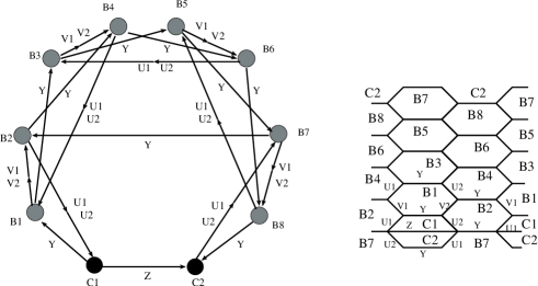
Figure 1: The quiver and brane tiling for $L^{195}(=Y^{54})$

We now describe some essential features of the $L^{abc}$ quiver theories, mainly reviewing their construction in terms of brane tilings [9]. The gauge dual to the geometry $AdS_{5}\times L^{abc}$ is a quiver gauge theory in which all gauge groups are $SU(N)$. The global symmetry of the theory is $U(1)_{F_{1}}\times U(1)_{F_{2}}\times U(1)_{B}\times U(1)_{R}$. The $U(1)_{F_{i}}$ are flavour symmetries and the $U(1)_{B}$ and $U(1)_{R}$ are baryon and R-symmetries respectively. The number of fields in the gauge theory is given by:

$$N_{g}=a+b\qquad N_{f}=a+3b$$ (6)

where $N_{g}$ is the number of gauge groups i.e. the number of nodes in the quiver diagram, and $N_{f}$ is the number of bifundamental chiral fields, i.e. the number of lines in the quiver. There are four classes of chiral bifundamentals. We call these classes $Y,Z,U_{1},U_{2}$. There are two additional classes of fields $V_{1},V_{2}$. Fields in a class share the same Baryon, Flavour and R-charges. The multiplicity of fields in each class is

$$mult[Y]=b\quad mult[Z]=a\quad mult[U_{1}]=d\quad mult[U_{2}]=c\quad mult[V_{1}]=b-c\quad mult[V_{2}]=c-a\ ,$$ (7)

i.e. there are $b$ distinct fields of type $Y$ carrying the same charges and so on.

There are $2b$ terms in the superpotential. A table listing all charges and multiplicities of each kind of field is found in [9]. There are 4 distinct types of nodes in the quiver:

$$A=U_{1}YV_{1}\cdot U_{1}YV_{1}\qquad B=V_{2}YV_{1}\cdot U_{1}YU_{2}\qquad C=YZ\cdot U_{1}U_{2}\qquad D=U_{2}YV_{2}\cdot U_{2}YV_{2}$$ (8)

This notation means that at a $B$ node for example, there are three bifundamentals, of type $V_{2},Y,V_{1}$ coming in and three bifundamentals of type $U_{1},Y,U_{2}$ going out or vice-versa.

Calling the multiplicity of each type of node in the diagram $(n_{A},n_{B},n_{C},n_{D})$, we have

$$n_{C}=2a\ ,\qquad n_{B}+2n_{A}=2(b-c)\ ,\qquad n_{B}+2n_{D}=2(c-a)\ ,$$ (9)

as relations among these positive integers. These relations do not completely fix the quiver. For most values of $(a,b,c)$, there is a line of solutions to these equations, with different gauge theories lying on this line related by Seiberg duality.

We can think instead of four tiles associated with these nodes and draw a brane tiling for the theory. The number of type $C$ tiles will be $n_{C}/2$. The other types occur $n_{A},n_{B}$ and $n_{D}$ times. Since there are only 4 kinds of tiles, there are only three kinds of terms

$$YU_{1}ZU_{2},\qquad YU_{1}V_{1},\qquad YU_{2}V_{2}\ ,$$ (10)

in the superpotential, the sign of each term given by the associated brane tiling [13, 9].

To extract the superpotential from the tiling, we colour the vertices in the brane tiling in alternating black or white. The terms in the superpotential are given by drawing clockwise loops around white nodes and anticlockwise loops around black nodes, contracting the fields on the edges crossed by the loop in the order determined by the colour of the node and assigning a minus sign to say black nodes and a positive sign to white nodes. See e.g. Figure 1 for a picture of the brane tiling for the space $L^{195}(=Y^{54})$ and the associated quiver.

3 $Y^{pq}$ quiver theories

Figure 2: The tiling for a general $Y^{pq}$ space

The Calabi-Yau cones $Y^{pq}$ with $p,q$ coprime with $p>q$ are a smooth subclass of the $L^{abc}$ geometries [5]. They are given by taking:

$$Q=(a,b,-c,-d)=(p-q,p+q,-p,-p)\ ,\qquad p,q>0\ {\rm coprime}\ ,$$ (11)

$Y^{1,0}$ being the conifold. The conditions on the number of nodes in the quiver for these $Y^{pq}$ geometries are

$$n_{C}=2(p-q)\ ,\qquad n_{B}+2n_{A}=2q\ ,\qquad n_{B}+2n_{D}=2q\ .$$ (12)

Thus we can choose $n_{A}=n_{D}=0$ so that we have only $C$ nodes and $B$ nodes, giving $n_{C}=2(p-q)$ and $n_{B}=2q$. The tiling for the gauge theory corresponding to $Y^{pq}$ is shown in Figure 2. These theories have wheel-like quiver diagrams (see Figure 4 for the quiver for $Y^{94}$). The superpotential $W$ in this case has $2(p+q)$ terms which can be read off the nodes of the tiling. The links in the quiver with one arrow represent single bifundamental fields, while the links with $k$ arrows represent $k$ fields that are bifundamentals under the same two gauge groups. The multiplicities of the quiver fields are

$$mult[Y]=p+q\ ,\quad mult[Z]=p-q\ ,\quad mult[U_{1}]=mult[U_{2}]=p\ ,\quad mult[V_{1}]=mult[V_{2}]=q\ .$$ (13)

In what follows, we discuss mesonic branches of the classical chiral ring of these $Y^{pq}$ quiver theories. In principle, our methods here should apply equally well to smooth $L^{abc}$ geometries that may be distinct from the $Y^{pq}$s which are a smooth subclass.

3.1 Mesonic sector of the chiral ring

In the gauge theory, the structure of the moduli space (defined by the equations of motion, $\partial W=0$) allows us to map a basis of gauge invariant commuting adjoint operators represented as irreducible loops (based at any one node) on the quiver to a basis set of $2p+5$ invariant monomials in the GLSM. Then the chiral ring of gauge invariant mesonic operators on the moduli space precisely reproduces the geometry of the singularity described as a toric variety in terms of invariant monomials satisfying relations. This is a natural generalization of the realization of the geometry of e.g. orbifold singularities from the moduli spaces of D-brane quiver theories [36, 1] . The structure of this map has built into it the following correspondence between the underlying variables of the geometry/GLSM and bifundamentals in the quiver

$$Y\ \sim\ z_{a}\equiv a\ ,\qquad\qquad Z\ \sim\ z_{b}\equiv b\ , \qquad\ \ V_{1}\ \sim\ z_{b}z_{d}\equiv bd\ ,$$

$$U_{1}\ \sim\ z_{c}\equiv c\ ,\qquad\qquad U_{2}\ \sim\ z_{d}\equiv d\ , \qquad\ \ V_{2}\ \sim\ z_{b}z_{c}\equiv bc\ .$$ (14)

We use this to identify quiver loops and GLSM monomials (we have for notational convenience, used $a,b,c,d$, for the GLSM fields and will continue to do so in what follows). As it stands, this is a many-to-one map, consistent with the baryon charges in the gauge theory mapping to the $U(1)$ charges in the GLSM.

Figure 3: The quiver for the supersymmetric conifold

We will first quickly review the familiar conifold [2, 3] from this point of view. The quiver in this case is shown in Figure 3: the theory has bifundamentals $A_{i}$ in the $(N,\bar{N})$ and $B_{j}$ in the $(\bar{N},N)$ of the $SU(N)\times SU(N)$ gauge group. The superpotential is $W={\lambda\over 2}\epsilon^{ij}\epsilon^{kl}\operatorname{tr}A_{i}B_{k}A_{j}B_{l}$. The four equations of motion $\partial_{i}W=0$ are of the form $A_{1}B_{1}A_{2}=A_{2}B_{1}A_{1}$. We define four gauge invariant operators $x_{k}\equiv A_{i}B_{j}$, which can be identified with the four irreducible closed loops on the quiver starting at the right node. Then we see using the equations of motion that these commute and satisfy the relation $x_{1}x_{4}=x_{2}x_{3}$, which is the familiar equation of the conifold as a hypersurface in ${\mathbb{C}}^{4}[x_{i}]$. In what follows, we will use essentially similar methods in the $Y^{pq}$ theories, where the incomplete intersection nature of the geometry makes the story somewhat more complicated.

We begin by discussing the GLSM and associated toric description for these geometries, first constructing a list of the invariant monomials modulo relations characterizing these geometries as toric varieties. There are $2p+5$ invariant monomials in the GLSM

$$abcd\ ,\quad abc^{2}\ ,\quad abd^{2}\ ,\quad a^{p}c^{(p-q)-k}d^{k},\quad b^{p}c^{(p+q)-l}d^{l},\qquad k=0\ldots p-q\ ,\ l=0\ldots p+q\ ,$$ (15)

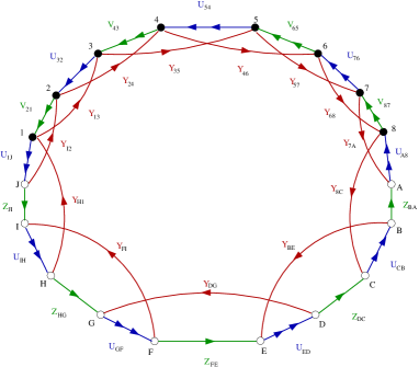
Figure 4: The quiver for $Y^{94}$

with some of the relations between these monomials being

$$(abc^{2})(abd^{2}) = (abcd)^{2}$$

$$(a^{p}c^{(p-q)-k_{1}}d^{k_{1}})\ (b^{p}c^{(p+q)-k_{2}}d^{k_{2}}) = (ab)^{p}c^{2p-n}d^{n}=(abc^{2})^{l_{1}}(abd^{2})^{l_{2}}(abcd)^{l_{3}}$$ (16)

$$(a^{p}c^{(p-q)-k}d^{k})(abc^{2}) = (a^{p}c^{(p-q)+2-k}d^{k-2})(abd^{2})=(a^{p}c^{(p-q)+1-k}d^{k-1})(abcd)$$

$$(b^{p}c^{(p+q)-k}d^{k})(abc^{2}) = (b^{p}c^{(p+q)+2-k}d^{k-2})(abd^{2})=(b^{p}c^{(p+q)+1-k}d^{k-1})(abcd)$$

where $k_{1}+k_{2}=l_{1}+l_{2}+l_{3}=n$ and $l_{3}=0$ or $1$.

Now let us move onto the quiver theory. Using the map (3.1) between the quiver gauge fields and GLSM fields, we can easily identify the invariant loops on the quiver. We label the nodes on the general $Y^{pq}$ quiver as $B1,\ldots,B2q,C1,\ldots,C2(p-q)$ going around in the clockwise direction. The generators are identified as follows:

$$abcd,abc^{2},abd^{2}\ \sim \ Y_{C2(p-q)B2}V^{1,2}_{B2B1}U^{1,2}_{B1C2(p-q)}$$ (17)

$$a^{p}c^{(p-q)-k}d^{k}\ \sim \ Y_{C2(p-q)B2}Y_{B2B4}Y_{B4B6}\ldots Y_{B(2q-2)B(2q)}Y_{B2qC3}U^{1,2}_{C3C2}Y_{C2C5}U^{1,2}_{C5C4}Y_{C4C7}\ldots$$

$$Y_{C2(p-q-1)B1}U^{1,2}_{B1C2(p-q)}$$

$$b^{p}c^{(p+q)-k}d^{k}\ \sim \ Z_{C2(p-q)C2(p-q)-1}U^{1,2}_{C2(p-q)-1C2(p-q)-2}Z_{C2(p-q)-2C2(p-q)-3}\ldots$$

$$Z_{C2C1}U^{1,2}_{C1B2q}V^{1,2}_{B2qB2q-1}U^{1,2}_{B2q-1B2q-2}V^{1,2}_{B2q-2B2q-3}\ldots V^{1,2}_{B2B1}U^{1,2}_{B1C2(p-q)}$$

These operators are in a sense the obvious generators: a set of triangles at the node $C2(p-q)$, a set of loops going clockwise and another going anticlockwise around the wheel.

Now we explain how these operators generate all possible paths on the quiver diagram. The $F$ equations generated by differentiating the superpotential with respect to $U$s and $V$s along the outside of the wheel set neighboring $UVY$ triangles or $UZVY$ squares equal to each other. But drawing paths on the wheel, we can go around the wheel in the clockwise direction or anticlockwise direction or insert triangles and squares. But the $F$ equations allow us to move all the squares and triangles around to the triangles on the $C2(p-q)$ node and we are left with a path written as a product of the generators above. For a more rigorous analysis, see section 3.2 where the case $Y^{32}$ is worked out in detail. The $F$ equations obtained by differentiating with respect to the $Y$ fields restrict the number of generators so that the generators in the quiver theory are in one-to-one correspondence with the invariants in the GLSM.

For convenience in exploiting the equations of motion, we label these by a concise notation as follows. First we suppress explicitly labeling the fields including their multiplicities (as in Figure 1): for example, both $Y_{C1,B1}$ and $Y_{B1,B3}$ are labeled $Y$ with the understanding that the specific field will be clear from the context. Then the set of generating loops (operators) is

$$Y11\ ,\ Y12\ ,\ Y21\ ,\ Y22\ ,\quad Y^{q+1}1Y1Y\ldots Y1\ ,\ Y^{q+1}1Y2Y\ldots Y2\ ,\ etc$$

$${}Z1Z\ldots 1Z\ 11\ 11\ 11\ 11\ 1\ ,\quad Z1Z\ldots 2Z\ 21\ 11\ 11\ 11\ 1\ ,\ etc\ ,$$ (18)

where the last set of gauge invariant loops is a potentially large list of operators. However there are several equations of motion for the various fields.

The action of these $F$ term constraints on the generators is simple in this notation. For instance from any of the $Y$s excepting $Y_{B7B2}$, we have equations of the form $V_{1}U_{1}=V_{2}U_{2}$. Thus using the above notation, for two neighbouring fields we have $11=22$. Similarly the other equations of motion imply that for two fields separated by a $Y$ or a $Z$ we have $1Z2=2Z1$ and $1Y2=2Y1$. These F-term equations cut down the number of distinct loops (operators) so that an arbitrary loop (operator) can be generated by a basis of loops, which is precisely the set of invariant monomials in the GLSM. Overall, it can be shown that there are three linearly independent triangle generators, $p-q+1$ clockwise loops $Y^{q+1}\ldots$ and $p+q+1$ anticlockwise loops $Z\ldots$. Thus the independent generators in the quiver theory are in one-to-one correspondence with the invariants in the GLSM.

The generators in the quiver also commute with each other. We show the commutation of the triangles, denoting $Y_{13}=\bar{Y}$ and $U^{1,2}_{32}$ as $\bar{1}$ or $\bar{2}$.

$$Y12Y21 = Y1\bar{Y}\bar{2}21=Y1\bar{Y}\bar{1}11=(Y11)^{2}$$ (19)

$$Y21Y12 = Y2\bar{Y}\bar{1}12=Y2\bar{Y}\bar{2}22=(Y22)^{2}=(Y11)^{2}$$ (20)

So we have $[Y12,Y21]=0$. The other triangle operators commute in a similar manner.

Suppose we multiply $triangle\ \times\ loop$, where by loop we mean one of the clockwise or anticlockwise loops generators listed above. The $F$ equations allow us to move the triangle around from the beginning of the loop to the end, so that we have $[\ triangle\ ,\ loop\ ]=0$.

Finally if we multiply $clockwise\ \times\ anticlockwise$, we will have a triangle where the two paths connect. As we move this triangle anticlockwise around the wheel, we collect more and more triangles, so that we can write this operator as a product of triangles: $clockwise\ \times\ anticlockwise\ =\ triangle^{p}$, where by $triangle^{p}$ we schematically represent the product of various triangle operators. We can also write $anticlockwise\ \times\ clockwise=triangle^{p}$ and we can show that we can take the same triangles to occur in both expressions. Therefore the loop generators also commute.

The generators in the quiver theory also satisfy the same relations as the invariants of the GLSM. We have shown above the relation satisfied by the triangles. We have also explained how the relation $clockwise\ \times\ anticlockwise\ =\ triangle^{p}$ comes about. These relations correspond to the relations (3.1) in the GLSM. The relations $loop\ \times\ triangle=loop^{\prime}\ \times\ triangle^{\prime}$ also follow from the $F$ term equations.

We see that the quiver gauge theory contains a set of commuting gauge invariant operators, represented as irreducible loops at a single node, that are in one-to-one correspondence with the $r(=2p+5)$ invariant monomials in the GLSM, and satisfy the same relations as the GLSM invariants (section 3.2 describes this explicitly for the $Y^{32}$ case). For an $SU(N)^{N_{g}}$ theory, these $r$ commuting operators are complex matrices that can be upper-triangulated by a gauge transformation. All gauge invariant functions of an upper-triangular matrix are symmetrized functions of the eigenvalues alone. Thus the quiver moduli space reproduces the geometry of the Calabi-Yau cone (or more precisely the symmetric product of $N$ copies of the Calabi-Yau cone, for $N$ branes), enabling us to recover the mesonic chiral ring of the gauge theory. With a view to doing this, consider first a $U(1)^{N_{g}}$ theory. The partition function over mesonic BPS states, using the state-operator map, counts “words” generated by the $2p+5$ invariant monomials $w_{j}$ in the GLSM

$$Z_{0}=\sum_{m_{j}}\left(\prod_{j=1}^{2p+5}w_{j}^{m_{j}}\right)\ \equiv\ \sum_{\sum_{i}n_{i}Q_{i}=0}\left(\prod_{i=1}^{4}z_{i}^{n_{i}}\right)\ .$$ (21)

The last expression here, involving the $z_{i}$, written in terms of the GLSM variables defining the toric variety, is equivalent to that in terms of the $w_{j}$ given by the holomorphic quotient. Replacing the $z_{i}$ by bosonic creation operators $a_{i}^{{\dagger}}$, we see that this is the partition function for a 4D (bosonic) harmonic oscillator with the constraint $\sum_{i}n_{i}Q_{i}=0$. Since gauge invariant operators of the $SU(N)^{N_{g}}$ theory are symmetrized functions of the eigenvalues, the Hilbert space for this theory is a symmetric product of $N$ copies of that of the $U(1)^{N_{g}}$ theory. The partition function is then that of $N$ bosons in a 4D harmonic oscillator potential with the constraint $\sum_{i}n_{i}Q_{i}=0$, and is given by the coefficient of $p^{N}$ in

$$Z=\prod_{\sum_{i}n_{i}Q_{i}=0}\ {1\over 1-pe^{-\sum_{i}n_{i}\beta_{i}}}\ .$$ (22)

This partition function has appeared in [27].

We now make a few comments on the bulk point of view. The $z_{i}$ carry the charges of the fields $Y,Z,U_{1},U_{2}$ respectively. Thus the chiral ring of a $Y^{pq}$ quiver theory can be interpreted as the set of all holomorphic functions in ${\mathbb{C}}^{4}$ which are invariant under the $U(1)$ action $z_{i}\to e^{iQ_{i}\alpha}z_{i}$. For any such function $f(z_{i})$, setting $f(z_{i})=0$ gives a holomorphic divisor of the Calabi-Yau cone. The corresponding giant graviton is then given by the intersection of this surface with the base, generalizing [21]. We have thus recovered in (22) the bulk partition function over all such cohomologically trivial, i.e. mesonic, giant gravitons propagating in the bulk $AdS_{5}\times L^{abc}_{5}$ spacetime. The fact that the gauge theory partition function agrees with that obtained from the bulk suggests a non-renormalization theorem for these BPS states.

In what follows we describe in detail the example $Y^{32}$. Similar analyses can be performed for other $L^{abc}$ spaces with smooth base 5-geometries, as well as other spaces obtained from e.g. ${\mathbb{C}}^{3}/{\mathbb{Z}}_{N}$ singularities (which are also toric), and perhaps more generally.

3.2 An example: $Y^{32}$

In this section, we illustrate explicitly the $Y^{32}$ theory, defined by $Q=(1,5,-3,-3)$. The $2p+5=11$ invariants here are

$$abcd\qquad abc^{2}\qquad abd^{2}$$

$$a^{3}c\qquad a^{3}d$$ (23)

$$b^{3}c^{5}\qquad b^{3}c^{4}d\qquad b^{3}c^{3}d^{2}\qquad b^{3}c^{2}d^{3}\qquad b^{3}cd^{4}\qquad b^{3}d^{5}$$

The resulting quiver and brane tiling are shown in Figure 5. The superpotential is given by:

$$W = Y_{32}U_{20}^{1}Z_{05}U_{53}^{2}-Y_{32}U_{20}^{2}Z_{05}U_{53}^{1}$$

$$\ +Y_{01}V_{12}^{2}U_{20}^{2}-Y_{01}V_{12}^{1}U_{20}^{1}+Y_{24}U_{41}^{1}V_{12}^{1}-Y_{24}U_{41}^{2}V_{12}^{2}$$

$$\ +Y_{13}V_{34}^{2}U_{41}^{2}-Y_{13}V_{34}^{1}U_{41}^{1}+Y_{45}U_{53}^{1}V_{34}^{1}-Y_{45}U_{53}^{2}V_{34}^{2}$$

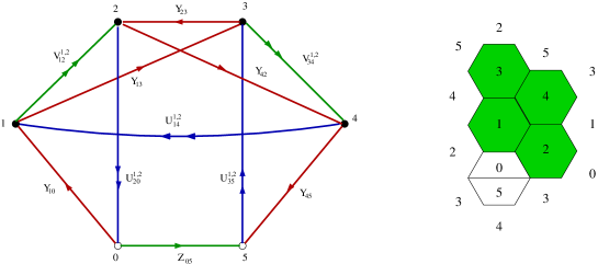
Figure 5: The quiver and brane tiling for $Y^{32}$

Each term here is a triangular or square loop on the quiver diagram. Every edge in the quiver appears in two such loops which appear with opposite sign in the superpotential. This makes the constraints ${\partial W\over\partial X}=0$, for any field $X$ in the quiver, easy to identify on the quiver diagram.

Every closed path on this quiver (i.e. every single trace gauge singlet) may be deformed using the $F$-term constraints so that it touches the $C$ node labelled $0$. We will consider the set of paths on the quiver diagram based (i.e. starting and ending) at the node $0$. We will show that all such operators and therefore all single trace operators in the chiral ring are generated by products of the operators shown in Figure 6.

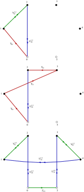
Figure 6: The basis of irreducible loops in the $Y^{32}$ quiver, based at node $0$.

First one may use the equations of motion to show that the independent loops of Figure 6 are in 1-to-1 correspondence with the invariants in the GLSM. There are four triangular paths $Y_{01}V_{12}^{1,2}U_{20}^{1,2}$, but the ${\partial W\over\partial Y_{10}}=0$ constraint sets $V_{12}^{1}U_{20}^{1}=V_{12}^{2}U_{20}^{2}$ so there are three independent triangles. These three paths correspond to the invariants $abcd$, $abc^{2}$ and $abd^{2}$ in the GLSM. The two “hourglass”-like operators $Y_{01}Y_{13}Y_{23}U_{20}^{1,2}$ correspond to the invariants $a^{3}c$ and $a^{3}d$ in the GLSM. Finally, since the lower indices are all fixed, denote the “rabbit”-like operators $Z_{05}U_{53}^{1,2}V_{34}^{1,2}U_{41}^{1,2}V_{12}^{1,2}U_{20}^{1,2}$ using only the upper indices as a sequence of five $1$s or $2$s as in $Z11111,Z12111$ etc.

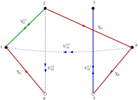
Figure 7: Decomposing loops of the $Y^{32}$ quiver beginning with $Y_{01}V_{12}\ldots$ into its irreducible loops.

Using the equations of motion ${\partial W\over\partial Y}=0$, we may remove any adjacent $2$s in an operator for example, $11221=11111$. We can also shift $2$s by 2 places using the equations of motion, so $12111=12221=11121$. Thus there are only six inequivalent independent operators of this form

$$Z21111=Z11211=Z11112\ ,\qquad\quad Z11111\ ,\qquad\quad Z12111=Z11121\ ,$$

$$Z21211=Z21112=Z11212\ ,\qquad\quad Z12121\ ,\qquad\quad Z21212\ ,$$ (25)

and they correspond to the six invariants $b^{3}c^{5-k}d^{k},\ k=0,\ldots,5$ in the GLSM. So the full list of adjoint operators we are considering is: $Y11,Y12,Y21,YYY1,YYY2$, and 6 operators of the form $Z11111,Z12111$, etc. This set is in 1-to-1 correspondence with the GLSM invariants.

Generators

Now we will show that all adjoints at node $0$ are generated by products of these 11 generating loops. The superscripts will not be important for this argument, so we will ignore them. Any operator, $A$, adjoint at node $0$ must begin with either $Y_{01}$ or $Z_{05}$ since these are the only two outgoing links at node $0$. These links must be similarly followed by similar outgoing links at either node $1$ or node $5$ respectively, and so on through all nodes in the loop, until the loop closes and returns to node $0$. We will try to construct an operator that cannot be reduced to generators.

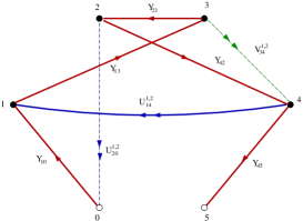
Figure 8: Decomposing loops of the $Y^{32}$ quiver beginning with $Y_{01}Y_{13}\ldots$ into its irreducible loops.

We first consider operators beginning with $Y_{01}$ and illustrate our argument in Figure 7. Suppose $A$ begins with $Y_{01}V_{12}Y_{24}\ldots$. If we next insert $U_{41}$ then we have $Y_{01}V_{12}Y_{24}U_{41}=(Y_{01}V_{12}U_{20})Y_{01}$ using the ${\partial W\over\partial V_{12}}=0$ equation, which is a generator times another loop. So to generate something that cannot be reduced, we must insert $Y_{45}U_{53}$ next. But this yields $Y_{01}V_{12}Y_{24}Y_{45}U_{53}$ which can be reduced to $Y_{01}V_{12}Y_{24}U_{41}Y_{13}$ using the ${\partial W\over\partial V_{34}}=0$ equation. But we just saw that if we leave node $4$ along $U_{41}$, then the operator can be reduced using the constraints. Thus if $A$ begins with $Y_{01}V_{12}Y_{24}$, then it can be reduced.

Next, we suppose $A$ begins with $Y_{01}Y_{13}\ldots$ and illustrate our argument in Figure 8. If we leave node $3$ along $V_{34}$ then we have $Y_{01}Y_{13}V_{34}=Y_{01}V_{12}Y_{24}$ by the ${\partial W\over\partial U_{41}}=0$ equations. This brings us back to the consideration of the previous paragraph, so instead we insert $Y_{32}$ and then $Y_{24}$ since $Y_{01}Y_{13}Y_{32}U_{20}$ is one of the generators shown in Figure 6. Then after inserting $Y_{24}$, we have $Y_{01}Y_{13}Y_{32}Y_{24}$ and we have arrived at node $4$. Now if we leave node $4$ along $U_{41}$, then we can use the ${\partial W\over\partial U_{41}}=0$ equation to reduce the path to generators:

$$Y_{01}Y_{13}Y_{32}Y_{24}U_{41}=(Y_{01}Y_{13}Y_{32}U_{20})Y_{01}$$ (26)

If instead we leave node $4$ along $Y_{45}$ to be followed by $U_{53}^{1,2}$, then we can use the ${\partial W\over\partial V_{34}^{1,2}}=0$ equation to replace the $Y_{45}U_{53}^{1,2}$ by $U_{41}^{1,2}Y_{13}$:

$$Y_{01}Y_{13}Y_{32}Y_{24}Y_{45}U_{53}=Y_{01}Y_{13}Y_{32}Y_{24}U_{41}Y_{13}$$ (27)

and we have just seen that this can be reduced.

These arguments have shown that every loop beginning with $Y_{01}$ can be reduced to the product of one of our 11 generators and some other loop. Similar considerations, which are illustrated in Figure 9 show that every operator beginning with $Z_{05}U_{53}\ldots$, may also be reduced to the product of one of the generators and some other loop.

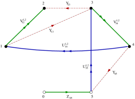
Figure 9: Decomposing loops of the $Y^{32}$ quiver beginning with $Z_{05}U_{53}\ldots$ into its irreducible loops.

Now iterating the results in the previous paragraph shows that all paths adjoint at the C node $0$ can be reduced to a product of the generators shown in Figure 6.

Commutation and GLSM relations

We will now show that the 11 generators satisfy the same relations as the invariants in the GLSM and that they commute. Consider first the triangular generators shown in Figure 6. The correspondence with the GLSM is:

$$abc^{2}\sim Y21\ ,\qquad abd^{2}\sim Y12\ ,\qquad abcd\sim Y11=Y22\ .$$ (28)

Then using the ${\partial W\over\partial V_{12}}=0$ equation and the ${\partial W\over\partial Y}=0$ equations, and denoting $Y_{24}$ by $\bar{Y}$ and $U_{41}^{1,2}$ by $\bar{1}$ and $\bar{2}$, we have:

$$Y21Y12 = Y2\bar{Y}\bar{1}12=Y2\bar{Y}\bar{2}22=Y22Y22\ ,$$

$$Y12Y21 = Y1\bar{Y}\bar{2}21=Y1\bar{Y}\bar{1}11=Y11Y11=Y22Y22\ ,$$ (29)

so that $[Y21,Y12]=0$ and $Y21Y12=(Y11)^{2}$ corresponding to $abc^{2}abd^{2}=(abcd)^{2}$. Also:

$$Y21Y11 = Y2\bar{Y}\bar{1}11=Y2\bar{Y}\bar{2}21=Y22Y21=Y11Y21\ ,$$

$$Y12Y22 = Y1\bar{Y}\bar{2}22=Y1\bar{Y}\bar{1}12=Y11Y12=Y22Y12\ .$$ (30)

So we also have $[Y21,Y11]=[Y12,Y11]=0$, i.e. the triangular generators commute and satisfy their GLSM relations.

Now we consider commutation between the triangular and hourglass shaped generators shown in Figure 6. We start with

$$(Y_{01}Y_{13}Y_{32}U_{20}^{a})(Y_{01}V_{12}^{b}U_{20}^{c})\ .$$ (31)

If $b=c$, then use the $F$-term constraints to set $a=c$. Now proceed:

$$(Y_{01}Y_{13}Y_{32}U_{20}^{a})(Y_{01}V_{12}^{b}U_{20}^{c}) = Y_{01}Y_{13}Y_{32}U_{20}^{a}Z_{05}U_{53}^{\bar{b}}Y_{32}U_{20}^{c}$$ (32)

where $\bar{b}$ is the opposite of $b$. Now use the ${\partial W\over\partial Z_{05}}=0$ and the ${\partial W\over\partial Y_{32}}=0$ equations to cyclically permute the label $a$ to the final position. Then we can show that

$$Y_{01}Y_{13}Y_{32}U_{20}^{\bar{b}}Z_{05}U_{53}^{c}Y_{32}U_{20}^{a} = (Y_{01}V_{12}^{b}U_{20}^{c})(Y_{01}Y_{13}Y_{32}U_{20}^{a})$$ (33)

so that $[Y_{01}Y_{13}Y_{32}U_{20}^{a},Y_{01}V_{12}^{b}U_{20}^{c}]=0$. So the hourglass and triangular generators commute.

Next we consider the commutation relations of the hourglass generators and the rabbit generators involving $Z_{05}$:

$$Z_{05}U_{53}^{1,2}V_{34}^{1,2}U_{41}^{1,2}V_{12}^{1,2}U_{20}^{1,2}$$ (34)

We will use the ${\partial W\over\partial U}=0$ and ${\partial W\over\partial V}=0$ constraints here and since they preserve the upper indices of the $U$s and $V$s (except the equations from $U_{20}$ and $U_{53}$), we will allow the lower index structure to be understood.

The $F$-term constraints imply the following relations for $a,b,\ldots,g$ taking values 1 or 2:

$$ZabcdeYfg=ZabYcdefg=ZaY\bar{b}Zcdefg=Y\bar{a}\bar{b}Zcdefg\ ,$$ (35)

If $fg=21$ and $ab=12$, then we obtain the commutation relations for the operators corresponding to $[b^{3}d^{5-k}c^{k},abc^{2}]=0$ for $k=2,\ldots,5$ in the GLSM. eg:

$$(Z12111)(Y21)=(Y21)(Z11121)\ .$$ (36)

Similarly if we take $fg=12$ and $ab=21$, then we obtain the relations $[b^{3}d^{5-k}c^{k},abd^{2}]=0$ for $k=0,\ldots,3$ in the GLSM. Using these relations and (35) we can show that the relations corresponding to $[b^{3}d^{4}c,abc^{2}]=0$ and $[b^{3}d^{5},abc^{2}]=0$ follow. The commutation relations corresponding to $[b^{3}d^{5-k}c^{k},abd^{2}]=0$ follow in the same manner by using (35) as above.

Setting $fg=11$ and $ab=11$ gives the relations corresponding to $[b^{3}d^{5-k}c^{k},abcd]=0$ for $k=1,\ldots,4$ in the GLSM and the two remaining commutation relations here follow as before by using commutation relations we have already proved:

$$(Z12121)(Y11) = (Y21)(Z12111)=(Z12111)(Y21)=(Y11)(Z12121)$$ (37)

We have thus shown that all rabbit-like generators commute with all triangular generators.

Certain relations from the GLSM can be recovered in gauge theory by using (35). If we let $fg=12$, and $ab=12$, then we obtain the four relations corresponding in the GLSM to $(b^{3}d^{5-k}c^{k})(abd^{2})=(abc^{2})(b^{3}d^{7-k}c^{k-2})$. Letting instead $fg=11$ and $ab=12,21$, we obtain 10 more relations corresponding to $(b^{3}d^{5-k}c^{k})(abd^{2})=(b^{3}d^{6-k}c^{k-1})(abcd)$ and $(b^{3}d^{5-k}c^{k})(abc^{2})=(b^{3}d^{4-k}c^{k+1})(abcd)$ in the GLSM.

Finally we consider the commutation relations of the hourglass operators and the rabbit like operators. Letting indices of the $Y$ fields be understood and denoting the hourglass operators as $Y^{3}1$ and $Y^{3}2$, we can use the $F$-term constraints to show that

$$(Y^{3}f)(Zabcde)=(Zf\bar{a}\bar{b}\bar{c}\bar{d})(Y^{3}e)\ .$$ (38)

Setting $a=e$ gives 10 of the hourglass-rabbit commutation relations and the remaining two commutation relations follow from these and previous relations. So all hourglasses commute with all rabbits.

The relations, corresponding to the 9 GLSM relations $(b^{3}d^{5-k}c^{k})(a^{3}c)=(abc^{2})^{l_{1}}(abd^{2})^{l_{2}}(abcd)^{l_{3}}$ where $l_{1}+l_{2}+l_{3}=3$ and to the 9 relations $(b^{3}d^{5-k}c^{k})(a^{3}d)=(abc^{2})^{l_{1}}(abd^{2})^{l_{2}}(abcd)^{l_{3}}$ where $l_{1}+l_{2}+l_{3}=3$ also now follow. So the generators in the gauge theory reproduce the the GLSM invariants and all their relations exactly.

4 Singularities in $L^{abc}$

In this section, we will describe aspects of $L^{abc}$ theories that have singular base 5-geometries. This happens if either of $a,b$ has common factors with either of $c,d$, as mentioned briefly earlier.

To see these singularities in the geometry ((see also [37]), we represent the full cone as a quotient (4) as $\left\{a|z_{a}|^{2}+b|z_{b}|^{2}=c|z_{c}|^{2}+d|z_{d}|^{2}\right\}//U(1)$.  The orbit of the $U(1)$ gauge symmetry, with action $(z_{a},z_{b},z_{c},z_{d})\to(e^{ia\theta}z_{a},e^{ib\theta}z_{b},e^{-ic\theta}z_{c},e^{-id\theta}z_{d})$, is an $S^{1}$ which is covered once for $\theta\in(0,2\pi)$ in the region where all $z_{i}$ are nonzero. But on surfaces where some of the $z_{i}=0$, the $S^{1}$ may be wrapped more than once. For example, suppose that $gcd(a,c)=h$. The $U(1)$ action on the surface $z_{b}=z_{d}=0$, given by $a|z_{a}|^{2}=c|z_{c}|^{2}$, is $(z_{a},0,z_{c},0)\to(e^{ik_{1}h\theta}z_{a},0,e^{-ik_{2}h\theta}z_{c},0)$ where $a=k_{1}h$ and $c=k_{2}h$. Then as $\theta$ goes from $0$ to $2\pi$, we wrap around the $S^{1}$ $h$ times. So we have a ${\mathbb{Z}}_{h}$ orbifold singularity extending in the whole $z_{b}=z_{d}=0$ plane.

Figure 10: The 3-dimensional toric fan for the singularity $Q_{i}$, defined by lattice points $e_{i}$. Also shown is the plane containing the $e_{i}$ for the singular case $L^{a,b,a}$.

The fact that we are dealing with toric singularities is useful, in particular in recovering the above conditions on the singularities of the base. The singularity (2) is represented by a toric cone in an integral $N$ lattice defined by four lattice points $e_{i}$ satisfying $\sum_{i}Q_{i}e_{i}=0$ (see Figure 10). The $e_{i}$ are coplanar (see e.g. [37]) iff $\sum_{i}Q_{i}=0$, i.e. $a+b=c+d$, in which case these are supersymmetric cones. Then the $e_{i}$ may be written in the form $e_{i}=(1,w_{i})$ so that we can draw the four vectors on a 2-plane. This is not unique since applying an $SL(3,{\mathbb{Z}})$ transformation to the vectors $e_{i}$ yields a cone describing the same geometry: a representation for the $e_{i}$ is (suppressing the third coordinate)

$$e_{4}=(0,0),\qquad e_{1}=(1,0),\qquad e_{2}=(-al,c)\ ,\qquad e_{3}=(ak,b)\ ,$$ (39)

where $k,l$ are two integers satisfying $bl+ck=1$ (we assume $b,c$ are coprime). The total $N$ lattice volume of the cone is $V_{cone}=a+b\ (=c+d)$, giving the number of gauge groups $N_{g}$ in the quiver. A toric cone of volume $V_{cone}>1$ is singular, so that there are $a+b$ subcones in the interior of the cone: subdividing by lattice points either in the interior of the cone or on the “walls” (faces) gives $a+b$ subcones each of volume $V_{subcone}=1$, i.e. a complete resolution representing a smooth space.

The fan encodes information on when the singularity is isolated (pointlike). The singularity (2) is isolated, i.e. the base space $X$ is smooth, if the toric fan does not contain any lattice points on its walls [41] (see also [37] in the context of these conifold-like singularities). This is algebraically equivalent to the condition that each of $a,b$ is coprime with each of $c,d$. It is easy to illustrate this if one of the $a,b,c,d$, say $b=1$. Then from the fan, we see that there are no lattice points on the $\{e_{2},e_{4}\}$ wall if $a,c$ are coprime: if there is a common factor $h$, then we can construct the $h-1$ lattice points  ${1\over h}\ [ke_{2}+(h-k)e_{4}],\ k=1,\ldots,h-1$, which lie on the $\{e_{2},e_{4}\}$ wall. These correspond to the $h-1$ twisted sector states of the $Z_{h}$ orbifold singularity described earlier. Similarly, there are no lattice points on the $\{e_{2},e_{3}\}$ wall if $a,1-c$ are coprime, i.e. $a$ is coprime with $d=a+1-c$. Doing this more generally shows that these are exactly the conditions we saw earlier for the orbifold singularities in the geometry.

4.1 $L^{aba}$

Figure 11: The quiver for $L^{121}$

This family of geometries is given by $Q=(\begin{array}[]{cccc}a&b&-a&-b\end{array})$, with $a,b$ coprime: in this case, a basis of invariant monomials is $x_{1}=z_{a}z_{c},\ x_{2}=z_{a}^{b}z_{d}^{a},\ x_{3}=z_{b}^{a}z_{c}^{b},\ x_{4}=z_{b}z_{d},$ satisfying the relation $x_{1}^{b}x_{4}^{a}=x_{2}x_{3}$. The toric cone for the geometries $L^{aba}$ is defined by the vectors $e_{i}=\{(0,0)\ ,(1,0)\ ,(0,a)\ ,(1,b)\}$ (see Figure 10). The lattice points on the faces of the cone reflect the fact that these spaces are singular on the base.

We consider here $L^{aba}$ with $gcd(a,b)=1$. This is a singular geometry with two orbifold singularities of order $a$ and $b$. The quiver diagram of the gauge theory is circular with $2a$ type $C$ nodes and $(b-a)$ type $A$ nodes (see Figures 11,  12). For our purposes, the charges of the fields will not be important, so we will label the fields on the quiver as $\{\bar{A},A,\bar{B},B,\bar{C},C,\ldots\}$ and $V_{i}$ on node $i$ if is a type $A$ node. We consider $L^{232}$ as an example. The general case is an obvious extension. We chose four adjoint generators at $C_{1}$:

$$x=A\bar{A}\qquad y=\bar{E}E\qquad s=ABCDE\qquad t=\bar{E}\bar{D}\bar{C}\bar{B}\bar{A}$$ (40)

The commutation relations follow as in the non-singular cases:

$$xs=A\bar{A}ABCDE=ABVCDE=ABCD\bar{D}DE=ABCDEA\bar{A}=sx$$ (41)

These four commuting adjoints at $C_{1}$ generate all gauge invariants passing through $C_{1}$ satisfying the $F$-term constraints. We can also see that these four adjoints satisfy $x^{2}y^{3}=st$:

$$x^{2}y^{3} = (A\bar{A})^{2}(\bar{E}E)^{3}=A\bar{A}AB(\bar{B}B)^{2}\bar{B}\bar{A}=ABV(\bar{B}B)^{2}\bar{B}\bar{A}=ABVC(\bar{C}C)\bar{C}\bar{B}\bar{A}$$ (42)

$$= ABCD\bar{D}\bar{C}C\bar{B}\bar{A}=ABCDE\bar{E}\bar{D}\bar{C}\bar{B}\bar{A}=st$$ (43)

These four generators reproduce the geometry completely, up to complex structure, but they do not generate all gauge invariant states of the gauge theory. Any path that touches three nodes and at least two neighboring $C$ nodes, can be moved around the graph using the $F$-term constraints, until it touches $C_{1}$. Therefore, all such paths are generated by the four adjoints $x,y,s,t$. Any path touching $A$ nodes, but not touching two neighboring $C$ nodes can be moved to the loop wrapping only $A\bar{A}$ by using the constraints. This path touches $C_{1}$ and is also generated by the adjoints $x,y,s,t$. Paths that touch only 2 $C$ nodes, however, cannot be deformed at all using the constraints, so we must count these operators separately.

The single trace gauge invariants are counted by traces of words made from $x,y,s,t$ satisfying $x^{2}y^{3}=st$ and the additional singlets $w_{n_{1}}=(C\bar{C})^{n_{1}}$, $u_{n_{2}}=(D\bar{D})^{n_{2}}$, $v_{n_{3}}=(V)^{n_{3}}$.

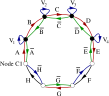
Figure 12: The quiver for $L^{aba}$

In the general $L^{aba}$ theory, with $gcd(a,b)=1$, paths touching $C_{1}$ are all generated by the four adjoints $x,y,s,t$ satisfying a constraint $x^{b}y^{a}=st$, where $x$ is the loop connecting $C_{1}$ to $A_{1}$, $y$ is the loop between $C_{1}$ and $C_{2}$ and $s,t$ are the loops around the whole graph in each direction. To demonstrate this relation, we label the lines before the $i^{th}$ gauge group as $A_{i},\bar{A_{i}}$, and label the lines between $C$ nodes as $C_{0},\ldots,C_{2(a-1)}$. Then we start with a set of loops at $C_{1}$ and we move them around the circle in the clockwise direction. We have:

$$(A_{1}\bar{A}_{1})^{b}(\bar{C}_{0}C_{0})^{a} =A_{1}(\bar{A}_{1}A_{1})^{b-1}V_{1}^{a}\bar{A}_{1}=A_{1}A_{2}(\bar{A}_{2}A_{2})^{b-2}\bar{A}_{2}V_{1}^{a}\bar{A}_{1}$$

$$=A_{1}A_{2}(\bar{A}_{2}A_{2})^{b-2}V_{2}^{a}\bar{A}_{2}\bar{A}_{1}$$

$$=A_{1}A_{2}\ldots A_{b-a}A_{b-a+1}(\bar{A}_{b-a+1}A_{b-a+1})^{a-1}\bar{A}_{b-a+1}V_{b-a}^{a}\bar{A}_{b-a}\ldots\bar{A}_{2}\bar{A}_{1}$$

$$=A_{1}A_{2}\ldots A_{b-a}A_{b-a+1}(C_{2(a-1)}\bar{C}_{2(a-1)})^{2a-1}\bar{A}_{b-a+1}\bar{A}_{b-a}\ldots\bar{A}_{2}\bar{A}_{1}$$

$$=A_{1}A_{2}\ldots A_{b-a}A_{b-a+1}C_{2(a-1)}C_{2(a-1)-1}\ldots C_{0}$$

$$\qquad\cdot\ \bar{C}_{0}\ldots\bar{C}_{2(a-1)-1}\bar{C}_{2(a-1)}\bar{A}_{b-a+1}\bar{A}_{b-a}\ldots\bar{A}_{2}\bar{A}_{1}$$

The generators $x,y,s,t$ do not generate all gauge invariant operators. We must also count the singlets $\omega_{n}^{i}=(C_{i}\bar{C_{i}})^{n}$ where $i=1,2,\ldots 2(a-1)$ corresponding to $C\bar{C}$ loops. Finally, given any path involving $V_{i}$, we can always remove $V_{i}$ from the path by using the $F$-term constraint equations if $V_{i}$ is contracted with any other line. So the only words including $V_{i}$ which we must count are the singlets $v_{k}^{i}=\operatorname{tr}V_{i}^{k}$, $i=1,\ldots b-a$.

There are $N_{g}-2$ extra singlet operators which are not generated by $x,y,s,t$. These are $\omega_{n}^{i}=(C_{i}\bar{C_{i}})^{n}$, where $i=1,2,\ldots,2(a-1)$ and $v_{k}^{i}=\operatorname{tr}V_{i}^{k}$, $i=1,\ldots,b-a$. The toric fan shows $a-1+b-1=N_{g}-2$ lattice points on the faces, corresponding to $N_{g}-2$ orbifold-like singularities, as we have described earlier. Thus we would expect that these extra operators in the gauge theory may be interpreted in the bulk as $N_{g}-2$ twisted sector closed string states. $L^{aba}$ has two orbifold-like singularities of order $a$ and $b$ respectively. These singularities have complex dimension one and twisted sector states in the bulk are restricted to move on these singularity planes. In other words, we expect such states to rotate only in this plane (i.e. angular momentum only normal to the plane): thus the charges of the twisted sector states associated to the $z_{i}$ normal to the singularity plane should be zero. Further, the charges associated to the $z_{i}$ covering the singularity plane should be given by the order of the orbifold singularity. In the gauge theory we have $a-1$ $C\bar{C}$ type operators of the form $YU_{1}$ and $a-1$ of the form $ZU_{2}$. This reproduces the spectrum of twisted states, with charges given in Table 1.

Table 1: $L^{aba}$: charges of operators

Field	Charge	Multiplicity
$V_{i}$	$(0,b,0,-b)$	$b-a$
$ZU_{2}$	$(0,b,0,-b)$	$a-1$
$YU_{1}$	$(a,0,-a,0)$	$a-1$

The partition function over ${1\over 2}$-BPS states will include these localized or twisted sector closed string states propagating in $AdS_{5}\times X^{5}$. It is clear from the discussion here that the partition function of the chiral ring will factor into the form:

$$Z_{bps}=Z_{gg}Z_{twist}$$ (44)

where $Z_{gg}$ is the partition function appearing in (22) and $Z_{twist}$ is the partition function over the twisted states. Since $\operatorname{tr}V_{i}^{N+1}$ is related to traces of lower powers by trace relations, we have exactly $N$ independent harmonic oscillators, $\operatorname{tr}V_{i}^{k},\ k=1\ldots N$, for each $i$, giving

$$Z_{twist}=\prod_{i=1}^{b-a}\prod_{n=1}^{N}{1\over 1-v_{i}^{n}}$$ (45)

where $v_{i}$ carries the charges of $V_{i}$.

It is interesting to wonder whether the whole chiral ring partition function might be recovered from a single bulk giant graviton quantization. In this context it is natural to imagine that twisted states with energies of order $N$ or higher puff up into D3-branes, analogous to giant gravitons, suggesting a generalization of [21] to include these localized giant gravitons.

5 Discussion

We have obtained the mesonic chiral ring partition function in ${\cal N}{=}1$ theories arising on the worldvolumes of D3-branes stacked at $Y^{pq},L^{abc}$ Calabi-Yau conical singularities. This agrees with their bulk interpretation as cohomologically trivial giant gravitons, suggesting a non-renormalization theorem for ${1\over 2}$-BPS states in these theories. The quiver theories for $L^{aba}$, with singular base geometries, contain extra operators not counted by the naive bulk partition function: these have a natural interpretation in terms of twisted states localized at the orbifold-like singularities in the bulk. It would be interesting to understand possible giant graviton interpretations of these localized states, possibly generalizing [21].

Our field theory techniques should apply to other quiver theories, such as those arising from D3-branes at ${\mathbb{C}}^{3}/\Gamma$ orbifold singularities (which are also toric), and perhaps more generally. The preliminary results of [42] suggest that our approach generalizes to baryonic operators in the quiver, corresponding to D3-brane giant gravitons wrapped on the non-contractible 3-cycle in the bulk.

It is worth mentioning that the counting problem addressed here shows agreement between the weak and strong coupling calculations even for large numbers of D3-brane giant gravitons. This suggests an underlying topological structure to the ${\cal N}{=}1$ chiral ring, preserved under the backreaction of the giant gravitons. For large numbers of giant gravitons, it would of course seem natural to cross over to a supergravity description, generalizing LLM [43] to geometries with $L^{abc}$ asymptotics: see [44] for some recent progress in this context. Quantization of the LLM solutions reproduced the large $N$ spectrum of $1/2$ BPS operators in $\mathcal{N}=4$ SYM [45],[46] and a similar quantization of LLM type solutions in $L^{abc}$ spaces might be expected to reproduce the large $N$ limit of the chiral ring partition functions in this paper. It would also be interesting to generalize the approach of [47] to shed light on matrix models and the emergence of geometry in the context of the ${\cal N}{=}1$ theories considered here.

Acknowledgments: It is a great pleasure to thank Shiraz Minwalla for innumerable discussions on this paper and collaboration on [42], as well as Davide Gaiotto for various discussions and collaboration in [42]. We would also like to thank Subhaneil Lahiri and Gautam Mandal for discussions.

References

- [1] M. Douglas, B. Greene, D. Morrison, “Orbifold resolution by D-branes”, [hep-th/9704151].
- [2] I. Klebanov, E. Witten, “Superconformal branes at a Calabi-Yau singularity”, [hep-th/9807080].
- [3] D. Morrison, M. R. Plesser, “Nonspherical horizons”, [hep-th/9810201].
- [4] J. Gauntlett, D. Martelli, J. Sparks, D. Waldram, “Supersymmetric solutions of M-theory”, [hep-th/0402153]; J. Gauntlett, D. Martelli, J. Sparks, D. Waldram, “Sasaki-Einstein metrics on ”, [hep-th/0403002]; “A new infinite class of Sasaki-Einstein manifolds”, [hep-th/0403038].
- [5] D. Martelli and J. Sparks, “Toric geometry, Sasaki-Einstein manifolds and a new infinite class of AdS/CFT duals,” Commun. Math. Phys. 262, 51 (2006) [arXiv:hep-th/0411238].
- [6] S. Benvenuti, S. Franco, A. Hanany, D. Martelli and J. Sparks, “An infinite family of superconformal quiver gauge theories with Sasaki-Einstein duals,” JHEP 0506, 064 (2005) [arXiv:hep-th/0411264].
- [7] S. Benvenuti and M. Kruczenski, “From Sasaki-Einstein spaces to quivers via BPS geodesics: L(p,q—r),” JHEP 0604, 033 (2006) [arXiv:hep-th/0505206].
- [8] A. Butti, D. Forcella and A. Zaffaroni, “The dual superconformal theory for L(p,q,r) manifolds,” JHEP 0509, 018 (2005) [arXiv:hep-th/0505220].
- [9] S. Franco, A. Hanany, D. Martelli, J. Sparks, D. Vegh and B. Wecht, “Gauge theories from toric geometry and brane tilings,” JHEP 0601, 128 (2006) [arXiv:hep-th/0505211].
- [10] M. Bertolini, F. Bigazzi and A. L. Cotrone, “New checks and subtleties for AdS/CFT and a-maximization,” JHEP 0412, 024 (2004) [arXiv:hep-th/0411249].
- [11] A. Hanany, P. Kazakopoulos and B. Wecht, “A new infinite class of quiver gauge theories,” JHEP 0508, 054 (2005) [arXiv:hep-th/0503177].
- [12] A. Hanany and K. D. Kennaway, “Dimer models and toric diagrams,” arXiv:hep-th/0503149.
- [13] S. Franco, A. Hanany, K. D. Kennaway, D. Vegh and B. Wecht, “Brane dimers and quiver gauge theories,” JHEP 0601, 096 (2006) [arXiv:hep-th/0504110].
- [14] D. Martelli, J. Sparks and S. T. Yau, “The geometric dual of a-maximisation for toric Sasaki-Einstein manifolds,” Commun. Math. Phys. 268, 39 (2006) [arXiv:hep-th/0503183].
- [15] S. Benvenuti and M. Kruczenski, “Semiclassical strings in Sasaki-Einstein manifolds and long operators in N= 1 gauge theories,” JHEP 0610, 051 (2006) [arXiv:hep-th/0505046].
- [16] A. Butti and A. Zaffaroni, “R-charges from toric diagrams and the equivalence of a-maximization and Z-minimization,” JHEP 0511, 019 (2005) [arXiv:hep-th/0506232].
- [17] A. Butti and A. Zaffaroni, “From toric geometry to quiver gauge theory: The equivalence of a-maximization and Z-minimization,” Fortsch. Phys. 54, 309 (2006) [arXiv:hep-th/0512240].
- [18] A. Hanany and D. Vegh, “Quivers, tilings, branes and rhombi,” arXiv:hep-th/0511063.
- [19] B. Feng, Y. H. He, K. D. Kennaway and C. Vafa, “Dimer models from mirror symmetry and quivering amoebae,” arXiv:hep-th/0511287.
- [20] J. McGreevy, L. Susskind, N. Toumbas, “Invasion of the giant gravitons from Anti deSitter space”, [hep-th/0003075]; M. Grisaru, R. Myers, O. Tafjord, “SUSY and Goliath”, [hep-th/0008015]; A. Hashimoto, S. Hirano, N. Itzhaki, “Large branes in AdS and their field theory duals”, [hep-th/0008016].
- [21] A. Mikhailov, “Giant gravitons from holomorphic surfaces”, [hep-th/0010206].
- [22] C. Beasley, “BPS branes from baryons”, [hep-th/0207125].
- [23] C. Romelsberger, “Counting chiral primaries in N = 1, d=4 superconformal field theories,” Nucl. Phys. B 747, 329 (2006) [arXiv:hep-th/0510060].
- [24] J. Kinney, J. Maldacena, S. Minwalla, S. Raju, “An index for four dimensional superconformal theories”, [hep-th/0510251].
- [25] I. Biswas, D. Gaiotto, S. Lahiri, S. Minwalla, “Supersymmetric states of N=4 Yang-Mills from giant gravitons”, [hep-th/0606087].
- [26] G. Mandal, N. V. Suryanarayana, “Counting -BPS dual giants”, [hep-th/0606088].
- [27] S. Benvenuti, B. Feng, A. Hanany and Y. H. He, “Counting BPS operators in gauge theories: Quivers, syzygies and plethystics,” arXiv:hep-th/0608050.
- [28] B. Feng, A. Hanany and Y. H. He, “Counting Gauge Invariants: the Plethystic Program,” arXiv:hep-th/0701063.
- [29] A. Hanany and C. Romelsberger, “Counting BPS operators in the chiral ring of N = 2 supersymmetric gauge theories or N = 2 braine surgery,” arXiv:hep-th/0611346.
- [30] A. Butti, D. Forcella and A. Zaffaroni, “Counting BPS baryonic operators in CFTs with Sasaki-Einstein duals,” arXiv:hep-th/0611229.
- [31] D. Martelli and J. Sparks, “Dual giant gravitons in Sasaki-Einstein backgrounds,” Nucl. Phys. B 759, 292 (2006) [arXiv:hep-th/0608060].
- [32] A. Basu and G. Mandal, “Dual giant gravitons in AdS(m) x Y**n (Sasaki-Einstein),” arXiv:hep-th/0608093.
-
[33]
S. Minwalla, Strings’06 talk, Beijing, China, June 2006,
http://strings06.itp.ac.cn/talk-files/minwalla.pdf . - [34] E. Witten, “Phases of theories in two dimensions”, [hep-th/9301042].
- [35] D. Morrison, M. R. Plesser, “Summing the instantons: quantum cohomology and mirror symmetry in toric varieties”, [hep-th/9412236].
- [36] M. Douglas, G. Moore, “D-branes, quivers and ALE instantons”, [hep-th/9603167].
- [37] K. Narayan, “Closed string tachyons, flips and conifolds,” JHEP 0603, 036 (2006), [hep-th/0510104]; “Phases of unstable conifolds”, to appear in Phys. Rev. D, [hep-th/0609017].
- [38] F. Cachazo, M. Douglas, N. Seiberg, E. Witten, “Chiral rings and anomalies in supersymmetric gauge theory”, [hep-th/0211170].
- [39] D. Berenstein, C. Herzog, P. Ouyang, S. Pinansky, “Supersymmetry breaking from a Calabi-Yau singularity”, [hep-th/0505029].
- [40] S. Pinansky, “Quantum deformations from toric geometry”, [hep-th/0511027].
- [41] E. Lerman, “Contact toric manifolds”, [math.SG/0107201].
- [42] D. Gaiotto, L. Grant, S. Minwalla, K. Narayan, work in progress.
- [43] H. Lin, O. Lunin, J. Maldacena, “Bubbling AdS space and 1/2 BPS geometries”, [hep-th/0409174].
- [44] E. Gava, G. Milanesi, K. S. Narain, M. O’Loughlin, “1/8 BPS states in AdS/CFT”, [hep-th/0611065].
- [45] L. Grant, L. Maoz, J. Marsano, K. Papadodimas and V. S. Rychkov, “Minisuperspace quantization of ’bubbling AdS’ and free fermion droplets,” [arXiv:hep-th/0505079].
- [46] L. Maoz and V. S. Rychkov, “Geometry quantization from supergravity: The case of ’bubbling AdS’,” [arXiv:hep-th/0508059].
- [47] D. Berenstein, “Large N BPS states and emergent quantum gravity”, [hep-th/0507203].