Bouncing and Accelerating Solutions in Nonlocal Stringy Models

Abstract:

A general class of cosmological models driven by a nonlocal scalar field inspired by string field theories is studied. In particular cases the scalar field is a string dilaton or a string tachyon. A distinguished feature of these models is a crossing of the phantom divide. We reveal the nature of this phenomena showing that it is caused by an equivalence of the initial nonlocal model to a model with an infinite number of local fields some of which are ghosts. Deformations of the model that admit exact solutions are constructed. These deformations contain locking potentials that stabilize solutions. Bouncing and accelerating solutions are presented.

1 Introduction

Field theories which violate the null energy condition (NEC) [1, 2] are of interest for the solution of the cosmological singularity problem and for the construction of cosmological dark energy models with the state parameter $w<-1$.

One of the first attempts to apply string theory to cosmology [3] was related to the problem of the cosmological singularity [2]. A possible way to avoid cosmological singularities consists of dealing with nonsingular bouncing cosmological solutions. In these scenarios the Universe contracts before the bounce [4]. Such models have strong coupling and higher-order string corrections are inevitable. It is important to construct nonsingular bouncing cosmological solutions in order to make a concrete prediction of bouncing cosmology.

Present cosmological observations [5] do not exclude an evolving dark energy (DE) state parameter $w$, whose current value is less than $-1$, that means the violation of the NEC (see [6, 7] for a review of DE problems and [8] for a search for a super-acceleration phase of the Universe).

A simple possibility to violate NEC is just to deal with a phantom field. The phantom field is unstable. There are general arguments that coupled scalar-gravity models violating the NEC are unstable ([9]-[13] and refs. therein). At the same time a phantom model could be an approximation to a nonlocal model that has no problems with instability [14]. A simple example of such a model is a model with a scalar nonlocal action $(e^{-\square_{g}}\phi)^{2}.$ In the second order derivative approximation $e^{-\square_{g}}\approx 1-\square_{g}$ this model is equivalent to a phantom one but does not have problems with instability. This type of models does appear in String Field Theory (SFT)(see [15] for a review) and in the p-adic string models [16]. The model with the particular kinetic term mentioned above is in fact realized in the p-adic string near a perturbative vacuum and is expected to be realized in the Vacuum String Field Theory (VSFT) [17].

The purpose of this paper is the study of this type of models. As a model we consider a SFT inspired nonlocal dilaton action. Distinguished features of the model are the invariance of the action under the shift of the dilaton field to a constant as well as a presence of infinite number of higher derivatives terms. A more general family of nonlocal models loosing the invariance of the nonlocal dilaton is also considered. For special values of the parameters the models describe linear approximations to the cubic bosonic or nonBPS fermionic SFT nonlocal tachyon models, or p-adic string models [14], [18]-[24]. The NonBPS fermionic string field tachyon nonlocal model has been considered as a candidate for the dark energy [14]. Several string-inspired and braneworld dark energy models have been recently proposed (see for example [25]-[27] and refs. therein). About a study of the tachyon dynamics with the Born-Infeld action see [28, 29, 30].

We discuss a possibility to stabilize the model that violates the NEC in the flat space-time at the cost of adding extra interaction terms in the Friedmann background. One of the lessons from a study nonlocal dynamics in the flat case is a sensitivity of the stability problem to the form of the interaction term [31, 32, 33, 34, 35, 18, 36]. We use the Weierstrass product to present the nonlocal field in terms of an infinite number of local fields [22]. Some of these local fields are ghosts, which violate the NEC and are unstable. The model is linear and admits exact solutions in the flat space-time. In non-flat case we get the same exact solutions after a deformation of the model. We used a similar approach to construct effective SFT inspired phantom models [37, 18, 38].

Another recently proposed model which violates the NEC and has higher derivatives is the ghost-condensation model [39]. Vector-scalar and tensor-scalar models that violate NEC and are stable in some region have been proposed in [40, 41], respectively.

The paper is organized as follows. In Section 2 we describe our strategy to the study of stringy inspired models. In Section 3 we present general solutions of the models in the flat case. Then we use some approximation to study these dynamics in the Friedmann metric and discuss cosmological properties of the constructed solutions.

2 Set up

In this paper we consider a model of gravity coupling with a nonlocal scalar field which induced by strings field theory

$$S=\int d^{4}x\sqrt{-g}\left(\frac{M_{p}^{2}}{2}R+\frac{M_{s}^{4}}{g_{4}}\left(\frac{1}{2}\phi\,F(-\square_{g}/M_{s}^{2})\phi-\Lambda^{\prime}\right)\right),$$ (1)

where $g$ is the metric, $\square_{g}=\frac{1}{\sqrt{-g}}\partial_{\mu}\sqrt{-g}g^{\mu\nu}\partial_{\nu}$, $M_{p}$ is a mass Planck, $M_{s}$ is a characteristic string scale related with the string tension $\alpha^{\prime}$, $M_{s}=1/\sqrt{\alpha^{\prime}}$, $\phi$ is a dimensionless scalar field (tachyon or dilaton), $g_{4}$ is a dimensionless four dimensional effective coupling constant related with the ten dimensional string coupling constant $g_{0}$ and the compactification scale. $\Lambda=\frac{M_{s}^{4}}{g_{4}}\Lambda^{\prime}$ is an effective four dimensional cosmological constant.

The form of the function $F$ is inspired by a nonlocal action appeared in string field theories. In particular cases

$$F(z)=-\xi^{2}z+1-ce^{-2z},$$ (2)

$\xi$ is a real parameter and $c$ is a positive constant. Using dimensional space-time variables and after a rescaling we can rewrite (1) for $F$ given by (2) as follows

$$\int d^{4}x\sqrt{-g}\left(\frac{m_{p}^{2}}{2}R+\frac{\xi^{2}}{2}\phi\,\square_{g}\phi+\frac{1}{2}(\phi^{2}-c\Phi^{2})-\Lambda^{\prime}\right),$$ (3)

where $\Phi=e^{\square_{g}}\phi$ and $m_{p}^{2}=g_{4}M_{p}^{2}/M_{s}^{2}$. Generally speaking the string scale does not coincide with the Plank mass [21, 23]. This gives a possibility to get a realistic value of $\Lambda$ [21].

The form of the term $(e^{\square_{g}}\phi)^{2}$ is analogous to the form of the interaction in the action for the string field tachyon in non-flat background [14], which is a generalization of the SFT tachyon interaction term in a flat background [42, 43, 15, 32, 33]. At some particular values of $\xi^{2}$ and $c$ this action appears in a linear approximation to SFT actions [44]-[48] and in a non-flat background has been considered in [14, 18, 19, 20, 24]. The case of the open Cubic Superstring Field Theory (CSSFT) [14, 20] tachyon corresponds to $\xi^{2}={}-1/\left(4\ln\left(\frac{4}{3\sqrt{3}}\right)\right)\approx 0.9556$ and $c=3$. We consider in detail action (3) at $c=1$, which is invariant under translation $\phi\to\phi+const$.

We take the metric in the form

$$ds^{2}={}-dt^{2}+a^{2}(t)\left(dx_{1}^{2}+dx_{2}^{2}+dx_{3}^{2}\right)$$ (4)

and get the following equation of motion for the space homogeneous scalar field $\phi$:

$$F(-{\cal D})\phi=0,$$ (5)

where

$${\cal D}\equiv{}-\partial_{t}^{2}-3H(t)\partial_{t},\quad H=\frac{\dot{a}}{a}\quad{\mbox{and}}\quad\dot{a}\equiv\partial_{t}a.$$ (6)

The Friedmann equations have the following form

$$\begin{split}3H^{2}&=\frac{1}{m_{p}^{2}}~{}{\cal E},\\ 3H^{2}+2\dot{H}&={}-\frac{1}{m_{p}^{2}}~{}{\cal P},\end{split}$$ (7)

where the energy and the pressure are obtained from the action (1) using standard formula

$$T_{\mu\nu}=-\frac{2}{\sqrt{-g}}\frac{\delta{S}}{\delta g^{\mu\nu}},\qquad T_{\mu\nu}=\mbox{diag}\{{\cal E},{\cal P},{\cal P},{\cal P}\}.$$ (8)

For the case of $F$ given by (2) the energy and the pressure have additional nonlocal terms ${\cal E}_{nl1}$ and ${\cal E}_{nl2}$ [33, 49, 50]

$$\begin{split}{\cal E}&={\cal E}_{k}+{\cal E}_{p}+{\cal E}_{nl2}+{\cal E}_{nl1}+\Lambda^{\prime},\\ {\cal P}&={\cal E}_{k}-{\cal E}_{p}+{\cal E}_{nl2}-{\cal E}_{nl1}-\Lambda^{\prime}.\end{split}$$ (9)

Nonlocal term ${\cal E}_{nl1}$ plays a role of an extra potential term and ${\cal E}_{nl12}$ a role of an extra kinetic term. The explicit form of the terms in the R.H.S. of (9) is

$$\begin{split}{\cal E}_{k}&=\frac{\xi^{2}}{2}(\partial\phi)^{2},\qquad{\cal E}_{p}={}-\frac{1}{2}\left(\phi^{2}-c(e^{\cal D}\phi)^{2}\right),\\ {\cal E}_{nl1}&=c\int_{0}^{1}\left(e^{(1+\rho){\cal D}}\phi\right)\left({}-{\cal D}e^{(1-\rho){\cal D}}\phi\right)d\rho,\\ {\cal E}_{nl2}&=-c\int_{0}^{1}\left(\partial e^{(1+\rho){\cal D}}\phi\right)\left(\partial e^{(1-\rho){\cal D}}\phi\right)d\rho.\end{split}$$ (10)

 

Our strategy is the following:

First, we study the dynamics of the model (3) in the flat case.

• We show that solutions have the form of plane waves. There are special values of parameters for which plane waves should be multiplied on linear functions. We calculate the energy and pressure on the corresponding solutions.

• We present dynamics of the nonlocal model in terms of an infinite number of local fields [22] and show that the energy and pressure densities of the nonlocal model are reproduced by the energy and pressure densities of the corresponding local models. For this purpose we use the Weierstrass product representation for the function $F$ in (1),

  $$F(z)=e^{f(z)}\prod_{n}\left(1-\frac{z}{\alpha^{2}_{n}}\right),$$ (11)

  where $\alpha^{2}_{n}$ are complex numbers, and represent the flat analog of (1) as

  $$S_{flat}=\frac{1}{2}\int d^{4}x\phi F(-\square)\phi\sim\frac{1}{2}\sum\left[\epsilon_{n}\psi_{n}e^{f(-\square)}(\square+\alpha_{n}^{2})\psi_{n}+c.c.\right],$$ (12)

  where $\square$ is the d’Alembertian in the flat space-time.

• We consider approximated models obtained by a truncation of number of local fields.

Then we consider the Friedmann Universe. There are two ways to study dynamics in the Friedmann metric:

• One can use the found expressions for the energy and pressure in the flat case, $E(\phi_{0})$ and $P(\phi_{0})$, to calculate the corresponding Hubble parameter $H_{0}$, then using this Hubble parameter calculate a perturbation of the flat solution of equation of motion and so on:

  $$\phi=\phi_{0}+\phi_{1}(H_{0})+...,~{}~{}~{}~{}~{}H=H_{0}(\phi_{0})+H_{1}(\phi_{0},\phi_{1})+...$$ (13)

• One can search for deformations of the model that admit the same exact solutions as in the flat case and try to argue that the deformed models describe the initial model with a good accuracy.

Both ways permit to find the first approximations to the models (5), (7). The first way have been used in [20]. In this paper we will follow the second way.

To this goal we use a representation of nonlocal dynamics given by action (1) in terms of local fields

$$\int d^{4}x\sqrt{-g}\left(\frac{m_{p}^{2}}{2}R+\frac{1}{2}\sum\left[\epsilon_{n}\psi_{n}e^{f(-\square_{g})}(\square_{g}+\alpha_{n}^{2})\psi_{n}+\Lambda^{\prime}+c.c.\right]\right).$$ (14)

We perform a deformation of this model by several steps. First, we consider an approximation to the model (14) in the form

$$\int d^{4}x\sqrt{-g}\left(\frac{m_{p}^{2}}{2}R+\sum\left[\frac{\epsilon_{n}}{2}\psi_{n}e^{f(\alpha_{n}^{2})}(\square_{g}+\alpha_{n}^{2})\psi_{n}+\Lambda^{\prime}+c.c.\right]\right)$$ (15)

Second, we restrict a number of local fields and, third, we add potentials of the order $1/m_{p}^{2}$ in which $\Lambda^{\prime}$ is also included:

$$\int d^{4}x\sqrt{-g}\left(\frac{m_{p}^{2}}{2}R+\sum\left[\frac{\epsilon_{n}}{2}\psi_{n}e^{f(\alpha_{n}^{2})}(\square_{g}+\alpha_{n}^{2})\psi_{n}+c.c.\right]-{\cal V}(\psi_{1},\dots,\psi_{n})\right).$$ (16)

such that solutions of the field equations in the non-flat case are the same as the flat case.

Finally, we find the corresponding scale factor $a(t)$ and study cosmological properties of approximated solutions to our model.

3 Flat Dynamics

3.1 General Solutions

3.1.1 Roots of the Characteristic Equation

In the flat case the action (1) has the following form:

$$S_{flat}=\frac{1}{2}\int d^{4}x\phi F(-\square)\phi.$$ (17)

Equation of motion on the space-homogeneous configurations (5) is reduced to the following linear equation:

$$F(\partial^{2})\phi=0.$$ (18)

A plane wave

$$\phi=e^{\alpha t}$$ (19)

is a solution of (18) if $\alpha$ is a root of the characteristic equation

$$F(\alpha^{2})=0.$$ (20)

For a case of $F$ given by (2) equation (18) has the following form

$$-\xi^{2}\partial^{2}\phi+\phi-ce^{-2\partial^{2}}\phi=0.$$ (21)

This equation has an infinite number of derivatives and can be treated as a pseudodifferential as well as an integral equation [35].

The corresponding characteristic equation:

$$F(\alpha^{2})\equiv-\xi^{2}\alpha^{2}+1-ce^{-2\alpha^{2}}=0$$ (22)

has the following solutions

$$\alpha_{n}={}\pm\frac{1}{2\xi}\sqrt{4+2\xi^{2}W_{n}\left({}-\frac{2ce^{-2/\xi^{2}}}{\xi^{2}}\right)},\quad n=0,\pm 1,\pm 2,...$$ (23)

where $W_{n}$ is the n-s branch of the Lambert function satisfying a relation $W(z)e^{W(z)}=z$. The Lambert function is a multivalued function, so eq. (22) has an infinite number of roots.

Parameters $\xi$ and $c$ are real, therefore if $\alpha_{n}$ is a root of (22), then the adjoined number $\alpha_{n}^{*}$ is a root as well. Note that if $\alpha_{n}$ is a root of (22), then $-\alpha_{n}$ is a root too. In other words, equation (22) has quadruples of complex roots

$$\alpha_{n,\pm\pm}=\pm\mathrm{Re}(\alpha_{n})\pm i\mathrm{Im}(\alpha_{n}).$$ (24)

If $\alpha^{2}=\alpha^{2}_{0}$ is a multiple root, then at this point $F(\alpha^{2}_{0})=0$ and $F^{\prime}(\alpha^{2}_{0})=0$. These equations give that

$$\alpha_{0}^{2}=\frac{1}{\xi^{2}}-\frac{1}{2},$$ (25)

hence $\alpha^{2}_{0}$ is a real number and all multiple roots of $F(\alpha^{2}_{0})=0$ are either real or pure imaginary. The multiple roots exist if and only if

$$c=\frac{\xi^{2}}{2e}e^{2/\xi^{2}}.$$ (26)

Real roots for any $\xi$ and $c$, except $\xi^{2}=0$ and $c=\infty$, are no more then double degenerated, because $F^{\prime\prime}(\alpha^{2}_{0})\neq 0$.

Summing up we note that according as the values of parameters $c$ and $\xi^{2}$ there exist the following types of the general real solution of (21):

• If $c\neq\frac{\xi^{2}}{2e}e^{2/\xi^{2}}$ and $c\neq 1$ then the general real solution is

  $$\phi=\sum_{n}R_{n}e^{m_{n}t}+\sum_{n}\left(C_{n}e^{\alpha_{n}t}+{C_{n}^{*}}e^{\alpha_{n}^{*}t}\right),$$ (27)

  where $R_{n}$ and $C_{n}$ are arbitrary real and complex numbers respectively.

• If $c=\frac{\xi^{2}}{2e}e^{2/\xi^{2}}>1$, then to get the general real solution one has to add to (27)

  $$\phi_{0}=\tilde{R}_{1}te^{m_{0}t}+\tilde{R}_{2}te^{-m_{0}t},\qquad m_{0}=\sqrt{\frac{1}{\xi^{2}}-\frac{1}{2}}\quad \xi^{2}<2,$$ if (28)

  $$\phi_{0}=\tilde{C}_{1}te^{i\alpha_{0}t}+\tilde{C}^{*}_{1}te^{-i\alpha_{0}t},\qquad\alpha_{0}=i\sqrt{\frac{1}{2}-\frac{1}{\xi^{2}}}\quad \xi^{2}>2.$$ if (29)

• If $c=1$ then to get the general real solution one has to add to (27)

  $$\phi_{0}=C_{1}t+C_{0},\qquad \xi^{2}\neq 2,$$ if (30)

  $$\phi_{0}=C_{3}t^{3}+C_{2}t^{2}+C_{1}t+C_{0},\qquad \xi^{2}=2.$$ if (31)

3.1.2 Real Roots of the Characteristic Equation

For some values of the parameters $\xi$ and $c$ eq. (22) has real roots. To mark out real values of $\alpha$ we will denote real $\alpha$ as $m$: $m=\alpha$.

To determine values of the parameters at which eq. (22) has real roots we rewrite this equation in the following form:

$$\xi^{2}=g(m^{2},c),\quad{\mbox{where}}\quad g(m^{2},c)=\frac{e^{2m^{2}}-c}{m^{2}e^{2m^{2}}}.$$ (32)

The dependence of $g(m,c)$ on $m$ for different $c$ is presented in Fig. (1). This function has a maximum at $m_{max}^{2}$

$$m_{max}^{2}=-\frac{1}{2}-\frac{1}{2}W_{-1}\left(-\frac{e^{-1}}{c}\right),$$ (33)

provided $c$ is such that $W_{-1}\left(-\frac{e^{-1}}{c}\right)<-1$, in the other words $0<c<1$.

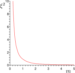
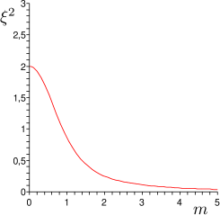
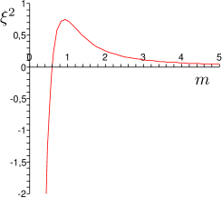
Figure 1: The dependence of function $g(m^{2},c)$, which is equal to $\xi^{2}$, on $m$ at $c=1/2$ (left), $c=1$ (center) and $c=2$ (right).

There are three different cases (see Fig. 1).

• If $c<1$, then eq. (22) has two simple real roots: $m=\pm m_{1}$ for any values $\xi$.

• If $c=1$, then eq. (22) has a zero root. Nonzero real roots exist if and only if $\xi^{2}>2$.

• If $c>1$, then eq. (22) has

  • no real roots for $\xi^{2}>\xi^{2}_{max}$, where

    $$\xi_{max}^{2}=\frac{1-ce^{-2m_{max}^{2}}}{m_{max}^{2}}={}-\frac{2}{W_{-1}(-e^{-1}/c)}$$ (34)

  • two real double roots $m=\pm m_{max}$ for $\xi^{2}=\xi^{2}_{max}$

  • four real single roots for $\xi^{2}<\xi^{2}_{max}$. In this case we have the following restriction on real roots: $m^{2}>\frac{1}{2}\ln c$.

3.1.3 Pure Imaginary Roots of the Characteristic Equation

For some values of the parameters $\xi$ and $c$ eq. (22) has a pair of pure imaginary roots. Let us introduce a new real variable $\mu=i\alpha$. From (21) we obtain

$$(\xi^{2}\mu^{2}+1)e^{-2\mu^{2}}=c.$$ (35)

This equation is equivalent to

$$\xi^{2}=\tilde{g}(\mu^{2},c),\quad\mbox{where}\quad\tilde{g}(\mu^{2},c)=\frac{c-e^{-2\mu^{2}}}{\mu^{2}e^{-2\mu^{2}}}.$$ (36)

The dependence of $\tilde{g}(\mu^{2},c)$ on $\mu$ for different $c$ is presented in Fig. 2.

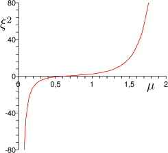
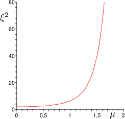
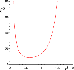
Figure 2: The dependence of function $\tilde{g}(\mu^{2},c)$, which is equal to $\xi^{2}$, on $\mu$ at $c=1/2$ (right), $c=1$ (center) and $c=2$ (left).

For different $c$ we have:

• For $c<1$ there are two real simple roots $\mu=\pm\mu_{1}$,

• For $c=1$ nonzero real roots exist only if $\xi^{2}>2$,

• For $c>1$ real roots exist if and only if

  $$\xi\geqslant\xi_{min}={}-\frac{2}{W_{0}\left(-\frac{e^{-1}}{c}\right)}.$$ (37)

  If $\xi=\xi_{min}$, then there exist two double real roots: $\mu=\pm\mu_{min}$, where

  $$\mu_{min}=\frac{1}{2}\sqrt{2+2W_{0}\left(-\frac{e^{-1}}{c}\right)}.$$ (38)

  At $\xi>\xi_{min}$ eq. (35) has four real simple roots.

3.1.4 Roots at the SFT inspired values on $\xi^{2}$ and $c$

Let us consider a special values of $\xi^{2}$ and $c$, which have been obtain in the SFT inspired cosmological model [14, 20]. From the action for the tachyon in the CSSFT [45] the following equation has been obtained [20]:

$$(-\xi_{0}^{2}\tilde{\alpha}^{2}+1)=3e^{-\tilde{\alpha}^{2}/4},$$ (39)

where

$$\xi_{0}^{2}={}-\frac{1}{4\ln\left(\frac{4}{3\sqrt{3}}\right)}\approx 0.9556.$$ (40)

Substituting $\tilde{\alpha}=2\sqrt{2}\alpha$, we obtain eq. (22) with $\xi^{2}=8\xi_{0}^{2}$ and $c=3$. From (26) it is follows that all roots are simple. We obtain that $\xi^{2}_{min}>\xi^{2}>\xi^{2}_{max}$, so there exist neither real roots nor pure imaginary roots.

3.2 Energy Density and Pressure

3.2.1 General Formula

Equation (21) has the conserved energy (compare with [49, 50, 18]), which is defined by the formula that is a flat analog of (9). The energy density is as follows:

$$E=E_{k}+E_{p}+E_{nl1}+E_{nl2},$$ (41)

where

$$E_{k}=\frac{\xi^{2}}{2}(\partial\phi)^{2},\qquad E_{p}=-\frac{1}{2}\phi^{2}+\frac{c}{2}\Phi^{2},$$ (42)

$$E_{nl1}=c\int_{0}^{1}\left(e^{-\rho\partial^{2}}\Phi\right)\left(\partial^{2}(e^{\rho\partial^{2}}\Phi)\right)d\rho,\qquad E_{nl2}=-c\int_{0}^{1}\left(\partial(e^{-\rho\partial^{2}}\Phi)\right)\left(\partial(e^{\rho\partial^{2}}\Phi)\right)d\rho.$$ (43)

For the pressure

$$P=E_{k}-E_{p}-E_{nl1}+E_{nl2},$$ (44)

we have the following explicit form

$$P=\frac{\xi^{2}}{2}(\partial\phi)^{2}+\frac{1}{2}\phi^{2}-\frac{c}{2}\Phi^{2}-c\int_{0}^{1}\left\{\left(e^{-\rho\partial^{2}}\Phi\right)\left(\partial^{2}(e^{\rho\partial^{2}}\Phi)\right)-\left(\partial(e^{-\rho\partial^{2}}\Phi)\right)\left(\partial(e^{\rho\partial^{2}}\Phi)\right)\right\}d\rho.$$ (45)

Let us calculate the energy density and pressure for the following solution

$$\phi=\sum_{n=1}^{N}C_{n}e^{\alpha_{n}t},$$ (46)

where $N$ is a natural number, $C_{n}$ are some constant and $\alpha_{n}$ are solutions to eq. (22).

For $N=1$ and

$$\phi=Ce^{\alpha t}$$ (47)

we obtain

$$E(Ce^{\alpha t}) = 0,$$ (48)

$$P(Ce^{\alpha t}) = C^{2}p_{\alpha}e^{2\alpha t}.$$ (49)

Hereafter we denote the energy density and pressure of function $\phi(t)$ as the functionals $E(\phi)$ and $P(\phi)$, respectively, and use the following notation

$$p_{\alpha}\equiv\alpha^{2}\left(\xi^{2}-2+2\xi^{2}\alpha^{2}\right).$$ (50)

For $N=2$ and

$$\phi=C_{1}e^{\alpha_{1}t}+C_{2}e^{\alpha_{2}t},$$ (51)

where $\alpha_{1}$ and $\alpha_{2}$ are different roots of (22) we have (see Appendix A for details)

$$E\left(C_{1}e^{\alpha_{1}t}+C_{2}e^{\alpha_{2}t}\right)=-2C_{1}C_{2}p_{\alpha_{1}},\qquad\mbox{at}\quad\alpha_{2}=-\alpha_{1},$$ (52)

and

$$E\left(C_{1}e^{\alpha_{1}t}+C_{2}e^{\alpha_{2}t}\right)=0,\qquad\mbox{at}\quad\alpha_{2}\neq{}-\alpha_{1}.$$ (53)

The pressure $P(\phi)$ for solution (51) is

$$P\left(C_{1}e^{-\alpha t}+C_{2}e^{\alpha t}\right)=\left(C_{1}^{2}e^{-2\alpha t}+C_{2}^{2}e^{2\alpha t}\right)p_{\alpha}.$$ (54)

In the general case we have

$$E\left(\sum_{n=1}^{N}C_{n}e^{\alpha_{n}t}\right)={}-2\sum_{n=1}^{N}\sum_{k=n+1}^{N}C_{n}C_{k}p_{\alpha_{n}}\delta_{\alpha_{n},-\alpha_{k}},$$ (55)

where

$$\delta_{\alpha_{n},-\alpha_{k}}=\begin{cases}1,&\alpha_{n}=-\alpha_{k},\\ 0,&\alpha_{n}\neq-\alpha_{k}.\end{cases}$$ (56)

Note that all summands in (55) are integrals of motion, therefore, we explicitly show that $E\left(\sum_{n=1}^{N}C_{n}e^{\alpha_{n}t}\right)$ is an integral of motion. From formula (55) we see that the energy density is a sum of the crossing terms. At the same time the pressure is a sum of ”individual” pressures and has no crossing term. In the case of an arbitrary finite number of summands the pressure is as follows:

$$P\left(\sum_{n=1}^{N}C_{n}e^{\alpha_{n}t}\right)=\sum_{n=1}^{N}C_{n}^{2}P\left(e^{\alpha_{n}t}\right)=\sum_{n=1}^{N}C_{n}^{2}p_{\alpha_{n}}e^{2\alpha_{n}t}.$$ (57)

If the parameters $\xi^{2}$ and $c$ are such that the characteristic equation (22) have double roots, then eq. (21) has the following solution

$$\phi_{0}(t)=B_{1}e^{\alpha_{0}t}t+C_{1}e^{\alpha_{0}t}+B_{2}e^{-\alpha_{0}t}t+C_{2}e^{-\alpha_{0}t},$$ (58)

where $B_{1}$, $B_{2}$, $C_{1}$ and $C_{2}$ are constants, $\alpha_{0}\neq 0$ is defined by (25). Using formulas (41) and (44) and substituting

$$\alpha_{0}=\frac{\sqrt{4-2\xi^{2}}}{2\xi},$$ (59)

we obtain

$$E(\phi_{0})={}-\frac{\left(\xi^{2}-2\right)}{3\xi^{2}}\left(3C_{1}B_{2}\sqrt{4-2\xi^{2}}\xi-3C_{2}B_{1}\sqrt{4-2\xi^{2}}\xi+8B_{1}B_{2}\left(2\xi^{2}-1\right)\right).$$ (60)

The pressure is as follows

$$\begin{split}P(\phi_{0})=&-\frac{\left(\xi^{2}-2\right)}{3\xi^{2}}\left(B_{2}e^{-\frac{t\sqrt{4-2\xi^{2}}}{\xi}}\left(B_{2}\left(8\xi^{2}-3t\sqrt{4-2\xi^{2}}\xi-4\right)-3C_{2}\xi\sqrt{4-2\xi^{2}}\right)+\right.\\ +&\left.B_{1}e^{\frac{t\sqrt{4-2\xi^{2}}}{\xi}}\left(3C_{1}\sqrt{4-2\xi^{2}}\xi+B_{1}\left(8\xi^{2}+3t\sqrt{4-2\xi^{2}}\xi-4\right)\right)\right).\end{split}$$ (61)

3.2.2 Energy Density and Pressure for real $\alpha$

As we have seen in Sect. 3.1.3 for some values of parameters $\xi$ and $c$ eq. (22) has real roots. We denote as $p_{m}$ the values of $p_{\alpha}$ for real $\alpha=m$,

$$p_{m}=m^{2}\left(\xi^{2}-2+2\xi^{2}m^{2}\right),$$ (62)

where $\xi^{2}$ is given by (32). For different values of $c$ the function $p_{m}$ is presented in Fig. 3.

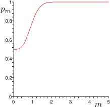
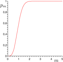
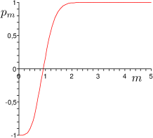
Figure 3: The dependence of $p_{m}$ on $m$ at $c=1/2$ (right), $c=1$ (center) and $c=2$ (left).

If and only if $c>1$, then there exists the interval of $0<m^{2}<m^{2}_{max}$ on which $p_{m}<0$. Some part of this interval is not physical because on this part $g(m^{2},c)<0$. The straightforward calculations show that

$$p_{m}=-\frac{\partial g(m^{2},c)}{\partial m^{2}}.$$ (63)

Therefore, at the point

$$m_{max}^{2}=-\frac{1}{2}-\frac{1}{2}W_{-1}\left(-\frac{e^{-1}}{c}\right),$$ (64)

we obtain $p_{m}(m_{max})=0$. We conclude that for $c>1$ and $\xi^{2}<\xi^{2}_{max}$ we have two positive roots of (22): $m_{1}$ and $m_{2}>m_{1}$, with $p_{m_{1}}<0$ and $p_{m_{2}}>0$.

The energy density and the pressure for solutions with real $\alpha$ one can calculate using formulas (55) and (57) and results are presented in Table 1.

$\phi$	$E$	$P$
$e^{\pm mt}$	0	$p_{m}e^{\pm 2mt}$
$\sinh(mt)$	$p_{m}/2$	$p_{m}\cosh(2mt)/2$
$\cosh(mt)$	${}-p_{m}/2$	$p_{m}\cosh(2mt)/2$

Table 1: Solutions, densities of energy and pressures for real $\alpha$

We see from Table 1 that odd solutions are physically meaningful, $E>0$, if $p_{m}$ is positive. Fig.3 shows that odd solutions are physical for $c<1$ and any $\xi^{2}$ and for $c>1$ only for $m^{2}>m_{max}^{2}$. The pressure corresponding to this solution is always positive.

Even solutions are physically meaningful if $p_{m}$ is negative. Therefore, even solutions are physical only for $c>1$ and $m^{2}<m_{max}^{2}$. The pressure corresponding to this solution is always negative. The equation of the state parameter for this solution is

$$w=-\cosh(2mt)<-1.$$ (65)

3.2.3 Energy Density and Pressure for pure imaginary $\alpha$

As we have seen in Sect.3.1.4 for some values of parameters $\xi$ and $c$ eq. (22) has only pair of pure imaginary roots. These solutions correspond to

$$\phi=C\sin(\mu(t-t_{0})).$$ (66)

On the solutions (66) the energy and pressure are given by

$$E(C\sin(\mu(t-t_{0}))) = \frac{C^{2}}{2}p_{\alpha}\equiv\frac{C^{2}}{2}\pi_{\mu},$$ (67)

$$P(C\sin(\mu(t-t_{0}))) = -\frac{C^{2}}{2}\pi_{\mu}\cos(2\mu(t-t_{0})),$$ (68)

where

$$\pi_{\mu}\equiv p_{i\mu}=\mu^{2}\left(2+2\xi^{2}\mu^{2}-\xi^{2}\right),$$ (69)

where $\xi^{2}$ is given by (36). $\pi_{\mu}$ as a function of $\mu$ for different values of $c$ is presented in Fig (4).

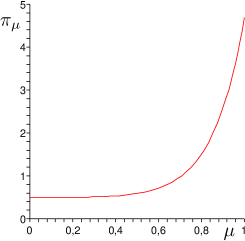
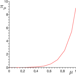
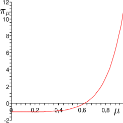
Figure 4: The dependence of $\pi_{\mu}$ on $\mu$ at $c=1/2$ (right), $c=1$ (center) and $c=2$ (left).

Note that $\pi_{\mu}$ for $c\leqslant 1$ is positive, however for $c>1$ is positive only for $\mu^{2}\geqslant\mu_{min}^{2}=\frac{1}{2}-\frac{1}{\xi^{2}}$. The equation of the state parameter for this solution is

$$w=-\cos(2\mu(t-t_{0})),~{}~{}\Rightarrow~{}~{}~{}|w|\leqslant 1.$$ (70)

3.2.4 Energy and Pressure in the case $c=1$

The energy density and pressure for solutions (30):

$$\phi_{1}(t)=C_{1}t+C_{0},$$ (71)

where $C_{0}$ and $C_{1}$ are arbitrary constants, are as follows

$$E(\phi_{1})=\left(\frac{\xi^{2}}{2}-1\right)C_{1}^{2},\qquad P(\phi_{1})=\left(\frac{\xi^{2}}{2}-1\right)C_{1}^{2}$$ (72)

and the state parameter $w\equiv P/E=1$.

The straightforward calculations show that pressure and energy density for more general solutions

$$\phi=\sum_{n=1}^{N}\tilde{C}_{n}e^{\alpha_{n}t}+\phi_{1}$$ (73)

are

$$E\left(\sum_{n=1}^{N}\tilde{C}_{n}e^{\alpha_{n}t}+\phi_{1}\right)=E\left(\sum_{n=1}^{N}\tilde{C}_{n}e^{\alpha_{n}t}\right)+E\left(\phi_{1}\right)$$ (74)

and

$$P\left(\sum_{n=1}^{N}\tilde{C}_{n}e^{\alpha_{n}t}+\phi_{1}\right)=P\left(\sum_{n=1}^{N}\tilde{C}_{n}e^{\alpha_{n}t}\right)+P\left(\phi_{1}\right).$$ (75)

Let, for example,

$$\phi(t)=\cosh(mt)+C_{1}t+C_{0}.$$

The corresponding energy density and pressure are:

$$E=-\frac{1}{2}p_{m}+\left(\frac{\xi^{2}}{2}-1\right)C_{1}^{2},\qquad P=\frac{1}{2}p_{m}\cosh(2mt)+\left(\frac{\xi^{2}}{2}-1\right)C_{1}^{2}.$$

In the case $\xi^{2}=2$ the root $\alpha=0$ is a double root of eq. (22), so eq. (21) has solutions (31):

$$\phi_{2}=C_{3}t^{3}+C_{2}t^{2}+C_{1}t+C_{0}.$$

We obtain:

$$E(\phi_{2})=4\left(3C_{1}C_{3}-C_{2}^{2}-6C_{3}^{2}\right),\qquad P(\phi_{2})=72C_{3}^{2}t^{2}+48C_{2}C_{3}t+4\left(C_{2}^{2}+3C_{1}C_{3}-6C_{3}^{2}\right).$$

3.2.5 Energy and pressure for complex $\alpha=r+i\nu$

For a decreasing solution

$$\phi(t)=e^{-rt}\cos(\nu t)$$ (76)

we have

$$E\left(e^{-rt}\cos(\nu t)\right)=0,$$ (77)

$$P\left(e^{-rt}\cos(\nu t)\right)=\frac{e^{-2rt}}{4}\left(p_{\alpha}e^{2i\nu t}+p_{\alpha^{*}}e^{-2i\nu t}\right).$$ (78)

Using general formulas (55) and (57) it is easy to find the energy and pressure for even and odd real solutions with complex $\alpha$. For example the energy and pressure for the even solution $\phi=\cosh(rt)\cos(\nu t)$ are as follows:

$$E(\cosh(rt)\cos(\nu t))=-\frac{1}{8}\left(p_{\alpha}+p_{\alpha^{*}}\right),$$ (79)

$$P(\cosh(rt)\cos(\nu t))=\frac{p_{\alpha}}{16}\left(e^{-2\alpha t}+e^{2\alpha t}\right)+\frac{p_{\alpha^{*}}}{16}\left(e^{-2\alpha^{*}t}+e^{2\alpha^{*}t}\right).$$ (80)

The equation of state parameter on the even solution is

$$w=-\frac{p_{\alpha}+p_{\alpha}^{*}}{p_{\alpha}\cosh(\alpha t)+p_{\alpha}^{*}\cosh(\alpha^{*}t)}.$$ (81)

3.3 Local Field Representation

3.3.1 Weierstrass product and Mode Decomposition for the Action

As in [22] we can present $F(-\square)$ in the action (1) as the Ostrogradski Representation. To this purpose let us construct the Weierstrass product for the function $F(z)$ of a complex variable $z$. Let us recall that a complex function $R(z)$ such that its logarithmic derivative $R^{\prime}(z)/R(z)$ is a meromorphic function regular in the point $z=0$, has simple poles and satisfies $|R^{\prime}(z)/R(z)|<C$, $z\in\Gamma_{n}$, $n=1,2,...$, can be presented as

$$R(z)=R(0)e^{\frac{R^{\prime}(0)}{R(0)}z}\prod\left(1-\frac{z}{z_{k}}\right)e^{z/z_{k}}.$$ (82)

$\Gamma_{n}$, $n=1,2,...$ is a set of special closed contours $\Gamma_{n}$ such that the point $z=0$ is in all $\Gamma_{n}$, $\Gamma_{n}$ is in $\Gamma_{n+1}$, and $S_{n}/d_{n}\leq C$, where $S_{n}$ is a length of the contour $\Gamma_{n}$, and $d_{n}$ is its distance from zero [51].

In the case of a more week requirement $|R^{\prime}(z)/R(z)|<M|z|^{p}$ $z\in\Gamma_{n}$, $n=1,2,...$ we have

$$R(z)=e^{f(z)}\prod\left(1-\frac{z}{z_{k}}\right)e^{Q_{k}(z)},\qquad Q_{k}(z)=\sum_{l=1}^{p}\frac{1}{l}\left(\frac{z}{z_{k}}\right)^{l},$$ (83)

where $f(z)$ is an entire function.

In the case of $R=F$ given by (2) the Weierstrass product can be written in the form

$$F(\alpha^{2})=e^{f(\alpha^{2})}\prod_{n}(\alpha^{2}-\alpha_{n}^{2}).$$ (84)

The function $f(z)$ in our case is

$$f(z)=A+\beta z,$$ (85)

where constants $A$ and $\beta$ are determined by $\xi$ and $c$. It will be shown that the equations of motion do not depend on values of $A$ and $\beta$.

It is convenient to pick out real roots in (84) and combine the complex conjugated roots:

$$F(\alpha^{2})=e^{A+\beta\alpha^{2}}\prod(\alpha^{2}-m_{k}^{2})\prod(\alpha^{2}-\alpha_{n}^{2})(\alpha^{2}-\alpha_{n}^{*2}),$$ (86)

where $m_{k}$ denote real roots. In Subsection 3.1 we have found the cases when real roots do exist.

In the case of simple roots the Lagrangian up to a total derivative can be presented as a sum of an infinite number of fields [52]–[55]

$${\cal L}=\frac{1}{2}\phi F(\partial^{2})\phi\sim\frac{1}{2}\sum\left[\epsilon_{n}\psi_{n}e^{f(\partial^{2})}(-\partial^{2}+\alpha_{n}^{2})\psi_{n}+c.c.\right],$$ (87)

where $\sim$ means equivalence up to a total derivative, $\epsilon_{n}$ are constants. It is the Ostrogradski representation. Note that for complex roots $\psi_{n}$ are complex.

3.3.2 Mode Decomposition for Energy Density and Pressure

It is instructive to present the formula for energy and pressure obtained in section 3.2. in terms of $\psi$ fields. All considerations below take place for nondegenerate roots.

According to a general procedure of construction of the energy and pressure we write a generalization of (87) to a non-flat case

$${\cal L}_{g}=\sum{\cal L}_{g}(\psi_{n}),\qquad{\cal L}_{g}(\psi_{n})=\frac{\epsilon_{n}}{2}\sqrt{-g}\psi_{n}e^{f(-\square_{g})}\left(\square_{g}+\alpha_{n}^{2}\right)\psi_{n},$$ (88)

and find

$$E_{\psi}=\sum_{n}E_{n},\qquad E_{n}=\frac{\epsilon_{n}}{2}\left(\dot{\psi_{n}}^{2}-\alpha_{n}^{2}\psi_{n}^{2}\right)e^{f(\alpha_{n}^{2})},$$ (89)

$$P_{\psi}=\sum_{n}P_{n},\qquad P_{n}=\frac{\epsilon_{n}}{2}\left(\dot{\psi_{n}}^{2}+\alpha_{n}^{2}\psi_{n}^{2}\right)e^{f(\alpha_{n}^{2})}.$$ (90)

The E.O.M. for $\psi_{n}$ is

$$(\partial^{2}-\alpha_{n}^{2})\psi_{n}=0$$ (91)

and its solutions are

$$\psi_{n}=A_{n}e^{\alpha_{n}t}+B_{n}e^{-\alpha_{n}t}.$$ (92)

For solutions (92) we obtain

$$E_{\psi} = 2\sum_{n}\alpha_{n}^{2}\epsilon_{n}A_{n}B_{n}e^{\beta\alpha_{n}^{2}},$$ (93)

$$P_{\psi} = \sum_{n}\epsilon_{n}\alpha_{n}^{2}\left(A^{2}_{n}e^{2\alpha_{n}t}+B_{n}^{2}e^{-2\alpha_{n}t}\right)e^{\beta\alpha_{n}^{2}}.$$ (94)

On the other hand according to (55) and (57) we have

$$E = -2\sum_{n}A_{n}B_{n}\alpha_{n}^{2}\left(\xi^{2}-2+2\xi^{2}\alpha_{n}^{2}\right),$$ (95)

$$P = \sum_{n}\left(A_{n}^{2}e^{-2\alpha_{n}t}+B_{n}^{2}e^{2\alpha_{n}t}\right)\alpha_{n}^{2}\left(\xi^{2}-2+2\xi^{2}\alpha_{n}^{2}\right).$$ (96)

Comparing (93),(94) and (95),(96) and using equation (22) we obtain that

$$E=E_{\psi},\qquad P=P_{\psi}$$ (97)

if and only if

$$\epsilon_{n}=-(2ce^{-2\alpha_{n}^{2}}+\xi^{2})e^{-\beta\alpha_{n}^{2}},$$ (98)

that is in accordance with general formula for $\epsilon_{n}$ [54, 22]. Note that we consider only simple roots $\alpha_{n}$.

3.4 Finite Order Derivative Approximation

3.4.1 Two types of approximations

There are two different types of finite order derivative approximations:

• a direct finite order derivative approximation

  $$L_{2k}(\alpha^{2})\equiv\sum_{n}^{k}a_{n}\alpha^{2n};$$ (99)

• an approximation by a finite number of terms in the Weierstrass product

  $$L^{(W)}_{2k}(\alpha^{2})\equiv f(\alpha^{2})\prod_{n}^{k}(\alpha^{2}-\alpha^{2}_{n}).$$ (100)

  We label roots so that $|\alpha_{n}|\leqslant|\alpha_{n+1}|$.

Locations of roots of the characteristic equation in the complex $\alpha$-plane are presented in Figure 5. One can see that structures of roots location for different values of $\xi$ look similar.

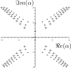
Figure 5: Roots for $c=1$ and $\xi=0$ (big crosses), $\xi=2$ (middle crosses) and $\xi=15$ (small crosses).

Let us consider the most simple case $\xi=0$, $c=1$, that corresponds to

$$L(\alpha^{2})\equiv L_{0,1}(\alpha^{2})=1-e^{-2\alpha^{2}}.$$ (101)

In this case all roots can be written explicitly

$$1-e^{-2\alpha^{2}}=2\alpha^{2}e^{-\alpha^{2}}\prod_{j=1}^{\infty}\left(1+\frac{\alpha^{4}}{\pi^{2}j^{2}}\right).$$ (102)

Note that all conclusions can be generalized on the case of arbitrary $\xi$ and $c$ such that all roots $\alpha_{n}$ are simple.

3.4.2 Direct Finite Order Approximation

In the second order derivative approximation we should keep in (21) with $c=1$, $\xi=0$ only the second derivatives

$$2\partial^{2}\phi=0.$$ (103)

This equation has the following solutions

$$\phi=C_{1}t+C_{2}.$$ (104)

These solutions correspond to roots $\alpha_{1}=0$.

In the fourth order derivative approximation eq. (22) at $c=1$ and $\xi=0$ is as follows

$$2\alpha^{2}-2\alpha^{4}=0$$ (105)

and has two solutions:

$$\alpha^{2}=0,\qquad\alpha^{2}=1.$$ (106)

We see that in the fourth order direct approximation the approximate equation (105) has a root ($\alpha=1$) that is absent in the initial equation (22).

The similar situation takes place for higher order approximations. The characteristic equation of the direct n-order approximation contains several artificial roots. The appearance of these roots is related to artificial roots of polynomial approximations of the function $f$ in the Weierstrass product (84). In Figure 6 we plot all roots of an n-order polynomial approximation of function $L_{0,1}(\alpha^{2})$ for n=20 and 40. We see that these polynomials have true roots as well as artificial roots that go to infinity when the order of the approximate polynomial increases.

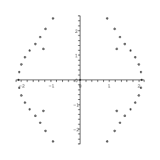
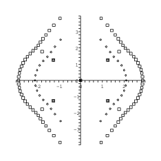
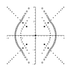
A.   B.   C.

Figure 6: A. Roots of the 20-th order approximation $L_{0,1;10}(\alpha)$ of the function $L_{0,1}(\alpha^{2})$ depicted by small diamonds. There are one root in the origin, 4 roots located on a ”cross” and 15 roots on two bow-like curves. B. Roots of the 40-th order approximations, $L_{0,1;20}(\alpha)$, and roots of $L_{0,1;10}(\alpha)$ depicted by small boxes and small diamonds, respectively. $L_{0,1,20}(\alpha)$ has one root in the origin, 8 roots located on a ”cross” and 4 of them coincide with true roots of $L_{0,1;10}(\alpha)$. Artificial roots of $L_{0,1,20}(\alpha^{2})$ are located on bigger ”bows” as compare with artificial roots of $L_{0,1,10}(\alpha^{2})$. C. Exact roots of $L_{0,1}(\alpha)$ are located on a cross and depicted by small crosses. The roots of the $L_{0,1;10}(\alpha)$ and $L_{0,1;20}(\alpha)$, are depicted by small diamonds and small boxes, respectively, as in A and B.

3.4.3 Finite Order Weierstrass Product Approximation

We consider an approximation to $L_{0,1}(\alpha^{2})$ that keeps only a finite number of terms in the Weierstrass product

$$L^{(W)}_{0,1,2+4k}(\alpha^{2})\equiv 2\alpha^{2}e^{-\alpha^{2}}\prod_{j=1}^{k}\left(1+\frac{\alpha^{4}}{\pi^{2}j^{2}}\right).$$ (107)

We call this approximation as (2k+1)-roots approximation. The corresponding Lagrangian is

$${\cal L}^{(W)}_{0,1,2+4k}\equiv\frac{1}{2}\phi\partial^{2}e^{-\partial^{2}}\prod_{j=1}^{k}\left(1+\frac{\partial^{4}}{\pi^{2}j^{2}}\right)\phi.$$ (108)

Let us consider one root approximation

$${\cal L}^{(W)}_{0,1,2}\equiv\frac{1}{2}\phi\partial^{2}e^{-\partial^{2}}\phi.$$ (109)

E.O.M. is

$$\partial^{2}e^{-\partial^{2}}\phi=0$$ (110)

and it has an unique solution (the same as E.O.M. of 2-nd order derivative approximation)

$$\phi=At+C.$$ (111)

The next approximation is 3 roots approximation

$${\cal L}^{(W)}_{0,1,6}\equiv\frac{1}{2}\phi\partial^{2}e^{-\partial^{2}}\left(1+\frac{\partial^{4}}{\pi^{2}}\right)\phi.$$ (112)

E.O.M. is

$$\partial^{2}\left(1+\frac{\partial^{4}}{\pi^{2}}\right)e^{-\partial^{2}}\phi=0\qquad\Leftrightarrow\qquad\partial^{2}\left(1+\frac{\partial^{4}}{\pi^{2}}\right)\phi=0$$ (113)

and it has the following solutions

$$\phi_{6}(t)=A_{1}t+\delta_{1}+A_{2}e^{\sqrt{\frac{\pi}{2}}\,t}\sin(\sqrt{\frac{\pi}{2}}\,t+\delta_{2})+A_{3}e^{-\sqrt{\frac{\pi}{2}}\,t}\sin(\sqrt{\frac{\pi}{2}}\,t+\delta_{3}),$$ (114)

where $A_{k}$ and $\delta_{k}$ are arbitrary constants.

The next approximation contains 4 extra roots

$${\cal L}^{(W)}_{0,1,10}\equiv\frac{1}{2}\phi\partial^{2}e^{-\partial^{2}}\left(1+\frac{\partial^{4}}{\pi^{2}}\right)\left(1+\frac{\partial^{4}}{4\pi^{2}}\right)\phi.$$ (115)

E.O.M. is

$$\partial^{2}\left(1+\frac{\partial^{4}}{\pi^{2}}\right)\left(1+\frac{\partial^{4}}{4\pi^{2}}\right)e^{-\partial^{2}}\phi=0$$ (116)

and it has the following solutions

$$\phi_{10}(t)=\phi_{6}(t)+A_{4}e^{\sqrt{\pi}\,t}\sin(\sqrt{\pi}\,t+\delta_{4})+A_{5}e^{-\sqrt{\pi}\,t}\sin(\sqrt{\pi}\,t+\delta_{5}).$$ (117)

It is obvious that solutions of the Weierstrass approximate equations reproduce a finite number of modes of the full equation.

If we restrict ourself to decreasing solutions

$$\phi_{10,\mbox{decr}}(t)=\delta_{1}+A_{3}e^{-\sqrt{\frac{\pi}{2}}\,t}\sin\left(\sqrt{\frac{\pi}{2}}\,t+\delta_{3}\right)+A_{5}e^{-\sqrt{\pi}\,t}\sin(\sqrt{\pi}\,t+\delta_{5})$$ (118)

we see that the last term can be ignored as compared with term first two terms.

We can see that the Weierstrass product approximation is more preferable than direct approximation, because there is no problem with extra roots. In the next section we will use the Weierstrass product approximation to construct local cosmological models.

4 Non-flat Dynamics

4.1 Modified Action

The goal of this section is to consider the nonlocal model (1) in the Friedmann Universe. To consider the dynamics in such a system we need to solve nonlinear Friedmann equations (7), which represent hopelessly complicated problem. From (7) we obtain the following nonlinear integral equation in $H(t)$:

$$\dot{H}={}-\frac{1}{2m_{p}^{2}}({\cal{P}}+{\cal{E}})=-\frac{1}{m_{p}^{2}}\left(\frac{\xi^{2}}{2}(\partial\phi)^{2}-c\int_{0}^{1}\left(\partial e^{(1+\rho){\cal D}}\phi\right)\left(\partial e^{(1-\rho){\cal D}}\phi\right)d\rho\right),$$ (119)

where ${\cal D}\equiv{}-\partial_{t}^{2}-3H(t)\partial_{t}$. There is no method to solve eq. (119), even if the function $\phi(t)$ is given.

As a first step to consider such a problem we would like to construct some effective exactly solvable models that can be consider as an approximation to the nonlocal model. To do this we use the finite order approximations, constructed by the Ostrogradski method. In other words we choose a special solution of eq. (21) and find the corresponding Ostrogradski approximation in the flat space-time. After we deform the obtained approximate model to the case of the Friedmann Universe, assuming that exact solutions in the Friedmann metric are coincide with exact solutions in the flat space-time. Note that the similar assumption has been used in the papers [37, 18, 38] to construct effective local models with exact solutions.

Our starting point is the Lagrangian (87). The corresponding action in the non-flat space-time is as follows:

$$S_{Ostr.}=\int d^{4}x\sqrt{-g}\left(\frac{m_{p}^{2}}{2}R+\sum_{n}\left[\frac{\epsilon_{n}}{2}\psi_{n}e^{\beta\alpha_{n}^{2}}(\square_{g}+\alpha_{n}^{2})\psi_{n}+c.c.\right]-{\cal V}(\psi_{1},\dots,\psi_{n})\right).$$ (120)

If the fields $\phi_{n}$ depend only on time and the metric is a spatially flat Friedmann metric, then we have the following equation for $\psi_{n}$

$$\epsilon_{n}\left({}{\cal D}+\alpha_{n}^{2}\right)\psi_{n}-e^{-\beta\alpha_{n}^{2}}{\cal V}_{\psi_{n}}^{\prime}=0\quad\Leftrightarrow\quad(2ce^{-2\alpha_{n}^{2}}+\xi^{2})\left({}{\cal D}+\alpha_{n}^{2}\right)\psi_{n}+{\cal V}_{\psi_{n}}^{\prime}=0,$$ (121)

where ${\cal V}^{\prime}_{\psi_{n}}$ is a derivative of ${\cal V}$ on ${\psi_{n}}$. Note that form of ${\cal V}(\psi_{1},\dots,\psi_{n})$ depends on choose of special solutions $\psi_{1}$, $\dots$, $\psi_{n}$. The form of ${\cal V}(\psi_{1},\dots,\psi_{n})$ is given below (Subsection 4.4).

The energy and the pressure density in the Friedmann metric have the form

$${\cal E}_{mod} = E_{\psi}+{\cal V},$$ (122)

$${\cal P}_{mod} = P_{\psi}-{\cal V},$$ (123)

where $E_{\psi}$ and $P_{\psi}$ are given by formulas (89) and (90) respectively. This means that the extra term ${\cal V}$ play a role of a potential term.

The Friedmann equations of motion are

$$\begin{split}3H^{2}&=\frac{1}{m_{p}^{2}}~{}\left(E_{\psi}+{\cal V}\right),\\ 3H^{2}+2\dot{H}&={}-\frac{1}{m_{p}^{2}}~{}\left(P_{\psi}-{\cal V}\right),\end{split}$$ (124)

Therefore

$$\dot{H}={}-\frac{1}{2m_{p}^{2}}\left(P_{\psi}+E_{\psi}\right).$$ (125)

We choose such ${\cal V}$ that $\psi_{k}$ in the non-flat case are the same as in the flat case. Using (93) and (94)) we get

$$\dot{H}=\frac{1}{2m_{p}^{2}}\sum_{n}\alpha_{n}^{2}\epsilon_{n}e^{\beta\alpha_{n}^{2}}\Bigl{(}A^{2}_{n}e^{2\alpha_{n}t}+2A_{n}B_{n}+B_{n}^{2}e^{-2\alpha_{n}t}\Bigr{)}.$$ (126)

Using (92) we can rewrite (126) as follows

$$\dot{H}=\frac{1}{2m_{p}^{2}}\sum_{n}\epsilon_{n}e^{\beta\alpha_{n}^{2}}\dot{\phi}_{n}^{2}={}-\frac{1}{2m_{p}^{2}}\sum_{n}\left(2ce^{-2\alpha_{n}^{2}}+\xi^{2}\right)\dot{\phi}_{n}^{2}.$$ (127)

Substituting values of $\epsilon_{n}$ (formula 98) and using formulas (55) and (57), we obtain that

$$\dot{H}=\frac{1}{2m_{p}^{2}}\left(\frac{\xi^{2}}{2}(\partial\phi)^{2}-c\int_{0}^{1}\left(\partial(e^{-\rho\partial^{2}}\Phi)\right)\left(\partial(e^{\rho\partial^{2}}\Phi)\right)d\rho\right)=\frac{1}{2m_{p}^{2}}(E(\phi)+P(\phi)),$$ (128)

where

$$\phi(t)=\sum_{n}\phi_{n}(t)=\sum_{n}\left(A_{n}e^{\alpha_{n}t}+B_{n}e^{-\alpha_{n}t}\right).$$ (129)

Therefore,

$$H(t)=\frac{1}{2m_{p}^{2}}\left(\sum_{n}2A_{n}B_{n}p_{\alpha_{n}}t-\sum_{n}\left(-\frac{A_{n}^{2}}{2\alpha_{n}}e^{-2\alpha_{n}t}+\frac{B_{n}^{2}}{2\alpha_{n}}e^{2\alpha_{n}t}\right)p_{\alpha_{n}}\right)+H_{0},$$ (130)

where $H_{0}$ is an integration constant and we assume the sum goes over the complex conjugated roots.

It is convenient to rewrite (127) as follows

$$\dot{H}={}-\frac{1}{2m_{p}^{2}}\sum_{n}\frac{p_{\alpha_{n}}}{\alpha_{n}^{2}}\dot{\phi}_{n}^{2}={}-\frac{1}{2m_{p}^{2}}\Bigl{(}(\xi^{2}-2)\sum_{n}\dot{\phi}_{n}^{2}+2\xi^{2}\sum_{n}\alpha_{n}^{2}\dot{\phi}_{n}^{2}\Bigr{)}.$$ (131)

Thus to obtain the crossing of cosmological constant barrier one should consider the case $\xi^{2}<2$ and the field $\phi(t)$, which consists of at least two modes. It is easy to see that $H(t)$ has no singular point at finite time. For some values of parameters we obtain bouncing solutions, which satisfy the conditions $H(0)=0$ and $\dot{H}(0)>0$.

In the following subsections we construct effective potentials for one-, two- and $N$-modes solutions. One-mode models can be consider as toy-models, whereas two-fields models are more realistic. Note that there are modern inflation models, for example [56, 57], which include two scalar fields (see also [58] and references therein). In this paper we describe a procedure to construct effective models and analyse only the simplest properties of them. More detail analysis and compare with the nonlocal model dynamic is a subject of our future investigations.

4.2 One Mode Solutions

4.2.1 One Real Root: General case

Let $\alpha$ is a real root of (22), without loss of generality we can assume $\alpha>0$. The corresponding scalar field is (see (92)) as follows

$$\psi(t)=Ae^{\alpha t}+Be^{-\alpha t}.$$ (132)

The function $\psi(t)$ is a solution of the following first order differential equation:

$$\dot{\psi}^{2}=\alpha^{2}\left(\psi^{2}-4AB\right).$$ (133)

Using superpotential method [59] (see also [37, 38]) we consider the Hubble parameter as a function of $\psi$:

$$H=W(\psi(t))\qquad\Rightarrow\qquad\dot{H}=\frac{dW}{d\psi}\dot{\psi}.$$ (134)

From (131) we obtain

$$\frac{dW}{d\psi}={}-\frac{p_{\alpha}}{2m_{p}^{2}\alpha^{2}}\dot{\phi}={}\mp\frac{p_{\alpha}}{2m_{p}^{2}\alpha}\sqrt{\psi^{2}-4AB}$$ (135)

and

$$W(\psi)=\mp\frac{p_{\alpha}}{2m_{p}^{2}\alpha}\left(\frac{\psi}{2}\sqrt{\psi^{2}-4AB}-2AB\ln\left(\alpha\left(\psi+\sqrt{\psi^{2}-4AB}\right)\right)\right)+H_{0}.$$ (136)

The corresponding potential ${\cal V}(\psi)$ is

$${\cal V}(\psi)=3m_{p}^{2}W^{2}-\frac{p_{\alpha}}{2\alpha^{2}}\dot{\psi}^{2}=3m_{p}^{2}W^{2}-\frac{p_{\alpha}}{2}\left(\psi^{2}-4AB\right).$$ (137)

We see that the potential depend on values of constants $A$ and $B$, more exactly depend on value of the production $AB$, and does not depend on sign of $W(\psi)$. The potential ${\cal V}(\psi)$ is not a polynomial, but in the limit of the flat space-time ($m_{p}^{2}\rightarrow\infty$) we obtain a quadratic polynomial. Note that in the case of the flat space-time one can eliminate constants $A$ and $B$ adding a constant to potential ${\cal V}(\psi)$, so in this case the equations of motion do not depend on these constants. In the following subsections we analyse in detail a few particular cases.

4.2.2 One Real Root: Decreasing Solution

Let us consider a simplest particular case:

$$\psi=\exp(-mt),$$ (138)

From (130) we have

$$H(t)=\frac{p_{m}}{4m_{p}^{2}m}e^{-2mt}+H_{0}.$$ (139)

Therefore to ensure that (138) and (139) solve the Friedmann equations we have to add to the action the following potential

$${\cal V}(\psi)=\frac{3}{16m_{p}^{2}m^{2}}p_{m}^{2}\psi^{4}+\frac{3p_{m}}{2m}H_{0}\psi^{2}-\frac{p_{m}}{2}\psi^{2}+3m_{p}^{2}H_{0}^{2}.$$ (140)

Let us note that one gets the same potential for the unbounded solution $\psi_{1}=\exp(mt)$.

The decreasing solution (138), (139) corresponds to the scale factor

$$a(t)=a_{0}\exp\left({}-\frac{p_{m}}{8m_{p}^{2}m^{2}}\exp(-2mt)+H_{0}t\right).$$ (141)

This solution has no singularities at finite $t$. It describes an increasing Universe only in the case $p_{m}<0$. As we have seen in Sect.3.2.2 the negative pressure is possible if $c>1$ and $m^{2}<m_{max}^{2}$ that takes place if $\xi^{2}\leq\xi_{max}^{2}$, where $\xi_{max}$ is given by (34).

4.2.3 One Real Root: Odd Solution

Let us consider a odd solution

$$\psi=\sinh(mt).$$ (142)

From (130) we have

$$H(t)={}-\frac{p_{m}}{8m^{2}_{p}m}\sinh(2mt)-\frac{p_{m}}{4m^{2}_{p}}t+H_{0}$$ (143)

and the potential for $H_{0}=0$ is

$${\cal V}(\psi)=\frac{p_{m}}{2}\left(-1+\frac{3p_{m}}{8m_{p}^{2}}\left(t+\frac{1}{2m}\sinh(2mt)\right)^{2}\right).$$ (144)

The potential as a function of $\psi_{2}$ is given by

$${\cal V}(\psi)=-\frac{p_{m}}{2}+\frac{3p^{2}_{m}}{16m_{p}^{2}m^{2}}\left[\psi^{2}(1+\psi^{2})+2\psi\sqrt{1+\psi^{2}}\mbox{arcsinh}(\psi)+\mbox{arcsinh}(\psi)^{2}\right].$$ (145)

The odd increasing solution (142), (143) corresponds to the scale factor

$$a(t)=a_{0}\exp\left({}-\frac{p_{m}}{16m^{2}_{p}m^{2}}\left(\cosh(2mt)+2m^{2}t^{2}\right)+H_{0}t\right).$$ (146)

The scale factor (146) has no singularity. It increases at large time if $p_{m}<0$.

4.2.4 One Pure Imaginary Root

Let us consider an odd solution

$$\psi=\sin(\mu t).$$ (147)

From (67), (68) and (125) we get explicitly the Hubble parameter

$$H(t)=\frac{\pi_{\mu}}{4m^{2}_{p}}t+\frac{\pi_{\mu}}{8\mu m^{2}_{p}}\sin(2\mu t)+H_{0}.$$ (148)

The potential for $H_{0}=0$ as a function of $\psi$ is given by

$${\cal V}(\psi)=\frac{1}{2}\pi_{\mu}+\frac{3\pi_{\mu}^{2}}{16m^{2}_{p}\mu^{2}}\left[\psi^{2}(1-\psi^{2})+2\psi\sqrt{1-\psi^{2}}\arcsin(\psi)+\arcsin(\psi)^{2}\right].$$ (149)

Note, that this formula is valued only for $\psi^{2}\leqslant 1$. On this region the potential (149) is convex and it has an unique minimum.

The odd periodic solution (147), (148) corresponds to the scale factor

$$a(t)=a_{0}\exp\left(-\frac{\pi_{\mu}}{16\mu^{2}m^{2}_{p}}\cos(2\mu t)+\frac{\pi_{\mu}}{8m^{2}_{p}}t^{2}+H_{0}t\right)$$ (150)

and we have an expansion with an acceleration if $\pi_{\mu}>0$. In this case at $H_{0}=0$ we obtain the bouncing solution.

4.3 Solutions with the crossing of cosmological constant barrier

4.3.1 Pair of Complex Roots

For the case of a complex root $\alpha=r+i\nu$ we consider the following real solution

$$\psi_{4}=\psi_{\alpha}+\psi_{\alpha^{*}},\qquad\mbox{where}\qquad\psi_{\alpha}=e^{-\alpha t},\qquad\psi_{\alpha^{*}}=e^{-\alpha^{*}t}.$$ (151)

From (130) we have

$$H(t)=\frac{1}{4m_{p}^{2}}\left[\frac{p_{\alpha}}{\alpha}e^{-2\alpha t}+\frac{p_{\alpha^{*}}}{\alpha^{*}}e^{-2\alpha^{*}t}+H_{0}\right]=\frac{1}{4m_{p}^{2}}\left[\frac{p_{\alpha}}{\alpha}\psi_{\alpha}^{2}+\frac{p_{\alpha^{*}}}{\alpha^{*}}(\psi^{*}_{\alpha^{*}})^{2}+H_{0}\right].$$ (152)

The corresponding potential is as follows

$$\begin{split}{\cal V}&=\frac{3}{16m^{2}_{p}}\Bigl{[}\alpha^{2}\left(\xi^{2}-2+2\xi^{2}\alpha^{2}\right)^{2}\psi_{\alpha}^{4}+\alpha^{*2}\left(\xi^{2}-2+2\xi^{2}\alpha^{*2}\right)\psi_{\alpha^{*}}^{4}+H_{0}^{2}+{}\\ {}&+2\alpha\alpha^{*}\left(\xi^{2}-2+2\xi^{2}\alpha^{2}\right)\left(\xi^{2}-2+2\xi^{2}\alpha^{*2}\right)\psi_{\alpha}^{2}\psi_{\alpha^{*}}^{2}+2H_{0}\left(\frac{p_{\alpha}}{\alpha}\psi_{\alpha}^{2}+\frac{p_{\alpha^{*}}}{\alpha^{*}}(\psi^{*}_{\alpha^{*}})^{2}\right)\Bigr{]}.\end{split}$$ (153)

From (152) it follows that

$$\dot{H}={}-\frac{1}{2m_{p}^{2}}\left[p_{\alpha}e^{-2\alpha t}+p_{\alpha^{*}}e^{-2\alpha^{*}t}\right]={}-\frac{e^{-2rt}}{2m_{p}^{2}}\Bigl{[}(p_{\alpha}+p_{\alpha^{*}})\cos(\nu t)+i(p_{\alpha}-p_{\alpha^{*}})\sin(\nu t)\Bigr{]}.$$ (154)

It is easy to check that $p_{\alpha^{*}}=p_{\alpha}^{*}$, so $q_{1}\equiv p_{\alpha}+p_{\alpha^{*}}$ and $q_{2}\equiv i(p_{\alpha}-p_{\alpha^{*}})$ are real numbers. Formula (154) can be rewrite in the following form:

$$\dot{H}={}-\frac{\sqrt{q_{1}^{2}+q_{2}^{2}}}{2m_{p}^{2}}e^{-2rt}\sin(\nu t+\gamma),$$ (155)

where $\gamma$ is defined by the following relations:

$$\sin(\gamma)=\frac{q_{1}}{\sqrt{q_{1}^{2}+q_{2}^{2}}},\qquad\cos(\gamma)=\frac{q_{2}}{\sqrt{q_{1}^{2}+q_{2}^{2}}}.$$ (156)

As known the state parameter

$$w=-1-\frac{2}{3}\frac{\dot{H}}{H^{2}},$$ (157)

so we obtain that $w$ crossing the barrier $w={}-1$ infinite number of times.

For example, in the case: $\xi^{2}=0$ and $c=1$, when $p_{\alpha}=-2\alpha^{2}$ and

$$\dot{H}=\frac{1}{m_{p}^{2}}\sum_{n}\dot{\phi}_{n}^{2}.$$ (158)

If we choose $\alpha=\sqrt{\pi}+i\sqrt{\pi}$, then $p_{\alpha}=-2\pi i$, $q_{1}=0$, $q_{2}=-4\pi$, $\gamma=\pi$ and

$$\dot{H}=\frac{1}{m_{p}^{2}}\left(\alpha^{2}e^{-2\alpha t}+(\alpha^{*})^{2}e^{-2\alpha^{*}t}\right)={}-\frac{4\pi}{m_{p}^{2}}e^{-\sqrt{\pi}t}\sin(\sqrt{\pi}t-\pi).$$ (159)

The Hubble parameter (152) corresponds to the following scale factor

$$a(t)=a_{0}\exp\left\{H_{0}t-\frac{1}{8m_{p}^{2}}\left[\frac{p_{\alpha}}{\alpha^{2}}e^{-2\alpha t}+\frac{p_{\alpha^{*}}}{\alpha^{*2}}e^{-2\alpha^{*}t}\right]\right\},$$ (160)

substituting the explicit formula for $p_{\alpha}$ and $p_{\alpha^{*}}$ we get

$$a(t)=a_{0}\exp\left\{H_{0}t-\left(\frac{(\xi^{2}-2)}{4m_{p}^{2}}\cos(2\nu t)-\frac{\xi^{2}e^{-2rt}}{2m_{p}^{2}}\left[(r^{2}-\nu^{2})\cos(2\nu t)-2r\nu\sin(2\nu t)\right]\right)\right\}.$$ (161)

We see that a late time expansion regime corresponds only to $H_{0}>0$ (compare with [20]). Let us note that a constant part of the Hubble parameter $H_{0}$ can be incorporated in a plane solutions [20]:

$$\psi_{n}(t)=A_{n}e^{\alpha_{n,H_{0}}t}+B_{n}e^{-\alpha_{n,H_{0}}t},$$ (162)

where $\alpha_{n,H_{0}}$ is related with $\alpha_{n}$ as

$$\alpha_{n,H_{0}}^{2}+3H_{0}\alpha_{n,H_{0}}=\alpha_{n}^{2}.$$ (163)

Using this approximations authors has been investigate the case of the SFT inspired values of parameters $\xi^{2}$ and $c$ and obtain a cosmic acceleration with a periodic crossing of the $w=-1$ barrier. In our paper we obtain the similar result for arbitrary values of $\xi^{2}$ and $c$. Note that for some particular values of these parameters we can obtain one-fold crossing of the $w=-1$ barrier.

4.3.2 Two Real Roots Solutions

The above-mentioned solutions for real roots $m_{n}$ correspond to monotonic behaviour of the Hubble parameter. To describe nonmonotonic behaviour let us consider the case of $c>1$ and $\xi^{2}<\xi^{2}_{max}$. There exist two real roots of (22) $m_{1}$ and $m_{2}$ such that that $|m_{1}|<|m_{2}|$. The corresponding solution to (21) is

$$\psi=\psi_{1}+\psi_{2},\quad\mbox{where}\quad\psi_{1}=Ae^{m_{1}t},\quad\psi_{2}=Be^{m_{2}t},$$ (164)

where $A$ and $B$ are constants. Without loss of generality we can put $A=1$.

Using (126) we obtain

$$\dot{H}={}-\frac{1}{2m_{p}^{2}}\Bigl{(}p_{m_{1}}e^{2m_{1}t}+B^{2}p_{m_{2}}e^{2m_{2}t}\Bigr{)}.$$ (165)

Let us analyze a possibility $\dot{H}=0$, which correspond to crossing of the cosmological constant barrier for the state parameter $w$. In Subsection 3.2.2 we have obtained that $p_{m_{1}}<0$ and $p_{m_{2}}>0$ (See Figs. 1 and 3). So, for any roots $m_{1}$ and $m_{2}$, there exist such real $B$ that $\dot{H}=0$ at the point $t=t_{1}$:

$$B={}\pm\sqrt{\frac{{}-p_{m_{1}}e^{2m_{1}t_{1}}}{p_{m_{2}}e^{2m_{2}t_{1}}}}.$$ (166)

We conclude that solutions (164) correspond to cosmological models with the crossing of $w={}-1$ barrier.

The Hubble parameter and the scale factor are as follows:

$$H={}-\frac{1}{4m_{p}^{2}m_{1}m_{2}}\left(p_{m_{1}}m_{2}e^{2m_{1}t}+B^{2}p_{m_{2}}m_{1}e^{2m_{2}t}\right)+H_{0},$$ (167)

$$a=a_{0}\exp\left(-\frac{1}{4m_{p}^{2}m_{1}^{2}m_{2}^{2}}\left(p_{m_{1}}m_{2}^{2}e^{2m_{1}t}+B^{2}p_{m_{2}}m_{1}^{2}e^{2m_{2}t}\right)+H_{0}t\right).$$ (168)

If $m_{1}>0$ and $m_{2}<0$, then at late time

$$\dot{H}\approx{}-\frac{1}{2m_{p}^{2}}p_{m_{1}}e^{2m_{1}t}>0$$ (169)

and

$$H\approx{}-\frac{1}{4m_{p}^{2}m_{1}}p_{m_{1}}e^{2m_{1}t}>0.$$ (170)

Using

$$H=W(\psi_{1},\psi_{2})=\frac{{}-1}{4m_{p}^{2}m_{1}m_{2}}\left(p_{m_{1}}m_{2}\psi_{1}^{2}+p_{m_{2}}m_{1}\psi_{2}^{2}\right)+H_{0},$$ (171)

we obtain the fourth degree polynomial potential

$${\cal V}(\psi_{1},\psi_{2})=3m_{p}^{2}\left(\frac{1}{4m_{p}^{2}m_{1}m_{2}}\left(p_{m_{1}}m_{2}\psi_{1}^{2}+p_{m_{2}}m_{1}\psi_{2}^{2}\right)-H_{0}\right)^{2}-\frac{1}{2}\left(p_{m_{1}}\psi_{1}^{2}+p_{m_{2}}\psi_{2}^{2}\right).$$ (172)

We can conclude that all solutions (164) correspond to cosmological models with the crossing of $w={}-1$ barrier. Let us remind in this context that models with a crossing of the $w=-1$ barrier are a subject of recent studies [40, 41, 60, 61, 62, 63]. Simplest models include two scalar fields (one phantom and one usual field, see [38, 64, 65] and refs. therein). In our case a nonlocality provides a crossing of the $w=-1$ barrier in spite of the presence of only one scalar field. This fact has a simple explanation. The crossing of the $w=-1$ in our case is driven by an equivalence of our nonlocal model to a set of local models some of which are ghosts.

4.4 Cosmological models for N-mode solutions

Let us construct a cosmological model, with $\dot{H}$, defined by (130). To do this we use the superpotential method [59]. We consider the Hubble parameter as a function (superpotential) of $\psi_{n}$: $H(t)=W(\psi_{1},\psi_{2},\dots,\psi_{N})$. To construct potential we use the simplest form of the superpotential

$$H(t)=W(\psi_{1},\psi_{2},\dots,\psi_{N})=\sum_{n=1}^{N}W_{n}(\psi_{n}).$$ (173)

Using formula

$$\dot{H}=\sum_{n=1}^{N}\frac{dW_{n}}{d\psi_{n}}\dot{\psi}_{n},$$ (174)

we obtain, that (127) is satisfied if

$$\frac{dW_{n}}{d\psi_{n}}={}-\frac{1}{2m_{p}^{2}}\sum_{n}\left(2ce^{-2\alpha_{n}^{2}}+\xi^{2}\right)\dot{\psi}_{n}.$$ (175)

In the case of simple roots $\alpha_{n}$ the solutions

$$\psi_{n}=A_{n}e^{\alpha_{n}t}+B_{n}e^{-\alpha_{n}t}$$ (176)

satisfy the following first order differential equation:

$$\dot{\psi}_{n}^{2}=\alpha_{n}^{2}\left(\psi_{n}^{2}-4A_{n}B_{n}\right).$$ (177)

So,

$$\frac{dW_{n}}{d\psi_{n}}={}-\frac{p_{\alpha_{n}}}{2m_{p}^{2}\alpha_{n}^{2}}\dot{\psi}_{n}={}\mp\frac{p_{\alpha_{n}}}{2m_{p}^{2}\alpha_{n}}\sqrt{\psi_{n}^{2}-4A_{n}B_{n}}$$ (178)

and

$$W_{n}(\psi_{n})=\mp\frac{p_{\alpha_{n}}}{2m_{p}^{2}\alpha_{n}}\left(\frac{\psi_{n}}{2}\sqrt{\psi_{n}^{2}-4A_{n}B_{n}}-2A_{n}B_{n}\ln\left(\alpha(\psi_{n}+\sqrt{\psi_{n}^{2}-4A_{n}B_{n}})\right)\right).$$ (179)

The corresponding potential ${\cal V}(\psi_{1},\dots,\psi_{n})$ is

$${\cal V}(\psi_{1},\dots,\psi_{n})=3m_{p}^{2}W^{2}-\sum_{n}\frac{p_{\alpha_{n}}}{2\alpha_{n}^{2}}\dot{\psi}_{n}^{2}=3m_{p}^{2}\left(\sum_{n}W_{n}\right)^{2}+\sum_{n}\frac{p_{\alpha_{n}}}{2}\left(\psi_{n}^{2}-4A_{n}B_{n}\right).$$ (180)

We see that the potential and does not depend on sign of $W$. The potential $V(\psi)$ is not a polynomial, but in the limit of the flat space-time ($m_{p}^{2}\rightarrow\infty$) we obtain a quadratic polynomial. Formula (180) is a straightforward generalization of (137). Note that the form of potential is not unique (compare with [38]).

5 Conclusions

We have studied linear nonlocal models which violate the NEC. The form of them is inspired by the SFT. These models have an infinite number of higher derivative terms and are characterized by two positive parameters, $\xi^{2}$ and $c$.

The model with $c=1$ is a toy nonlocal model for the dilaton coupling to the gravitation field. A distinguished feature of it is the invariance under the shift of the dilaton field to a constant.

For particular cases of the parameters $\xi^{2}$ and $c$ the corresponding actions describe linear approximations to the bosonic [44, 32] and nonBPS fermionic [46] cubic SFT as well as to the nonpolynomial SFT [47, 48].

The case $\xi=0$ corresponds to a linear approximation to the p-adic string [16]. Let us note that recently a p-adics string inflation model has been considered [23].

In the flat case all solutions of the equation of motion are plane waves and are controlled by roots of the characteristic equation. Our characteristic equation has complex distinctive simple roots. In some particular cases there are single or double roots, which are real or pure imaginary. The energy on plane waves is equal to zero except for the cases of couples of roots $(\alpha,-\alpha)$. The pressure is a sum of one mode pressures. The pressure for the one plane wave corresponding to a real root can be positive or negative depending on parameters of the theory. For $c\leq 1$ the one mode pressure is positive and for $c>1$ it could be negative or positive.

To study cosmological applications we have investigated the behaviour of the models in the Friedmann background. We have performed this study within an approximation scheme. A simplest approximation is a local field approximation (or a mechanical analogous model in a terminology of [18]). On an example of the free flat case we have shown that in special cases we can use a local two derivatives approximation, but the next derivative approximations exhibit artifacts. Followed [22] we have used the Weierstrass product representation to study finite mode approximations. As was noted in [22] a straightforward application of the Ostrogradski method to these approximations indicates that energies are unbounded (an eigenvalue problem for the unbounded hyperbolic Klein-Gordon equation on manifolds is solved in [66]) and it is expected [22] that an incorporation of non-flat metric or nonlinear terms could drastically change the situation.

A distinguished cosmological property of these models is a crossing of the phantom divide [20, 24]. But there are also possibilities for other types of behaviour. Namely, the toy dilaton model possesses decreasing solutions describing asymptotical flat Universes (adding a cosmological constant modifies these solutions to near-de Sitter solutions). It also has odd bouncing solutions describing a contracting Universes meanwhile even bouncing solutions are forbidden. For special values of parameters corresponding to tachyon SFT models there are even bouncing solutions with an accelerated expansion.

We have shown that for some particular cases there are deformations of the model such that exact solutions of the linear problem are inherited by nonlinear non-flat ones. This is similar to what was done before for local models [37, 67, 68]. A stability of exact solutions in local models has been studied in [37]. We will study stability of our solutions in the future work.

Appendix A Calculations of Nonlocal Energy Density and Pressure on Plane Waves

In this appendix we calculate the energy density and pressure for the following solution

$$\phi=Ae^{\alpha_{1}t}+Be^{\alpha_{2}t},$$ (181)

where $\alpha_{1}$ and $\alpha_{2}$ are different roots of (22). We have

$$E(Ae^{\alpha_{1}t}+Be^{\alpha_{2}t})=E(Ae^{\alpha_{1}t})+E(Be^{\alpha_{2}t})+E_{cross}(Ae^{\alpha_{1}t},Be^{\alpha_{2}t})=ABE_{cross}(e^{\alpha_{1}t},e^{\alpha_{2}t}),$$ (182)

where the functional $E_{cross}$ is defined as follows:

$$E_{cross}(\phi_{1},\phi_{2})=\xi^{2}\partial\phi_{1}\partial\phi_{2}+\phi_{1}\phi_{2}+c\Phi_{1}\Phi_{2}+{}$$

$${}+c\int_{0}^{1}\left[\left(e^{-\rho\partial^{2}}\Phi_{1}\right)\partial^{2}\left(e^{-\rho\partial^{2}}\Phi_{2}\right)+\left(e^{-\rho\partial^{2}}\Phi_{2}\right)\partial^{2}\left(e^{-\rho\partial^{2}}\Phi_{1}\right)\right]d\rho-{}$$

$${}-c\int_{0}^{1}\left[\partial\left(e^{-\rho\partial^{2}}\Phi_{1}\right)\partial\left(e^{-\rho\partial^{2}}\Phi_{2}\right)+\partial\left(e^{-\rho\partial^{2}}\Phi_{2}\right)\partial\left(e^{-\rho\partial^{2}}\Phi_{1}\right)\right]d\rho,$$

$$\Phi_{1}\equiv e^{{}-\partial^{2}}\phi_{1},\qquad\Phi_{2}\equiv e^{{}-\partial^{2}}\phi_{2}.$$

For $\phi_{1}=e^{\alpha_{1}t}$ and $\phi_{2}=e^{\alpha_{2}t}$ we have

$$E_{cross}(e^{\alpha_{1}t},e^{\alpha_{2}t})=e^{(\alpha_{1}+\alpha_{2})t}\Big{\{}\alpha_{1}\alpha_{2}-1+ce^{({}-\alpha_{1}^{2}-\alpha_{2}^{2})}+{}$$

$${}+ce^{-\alpha_{1}^{2}-\alpha_{2}^{2}}\int_{0}^{1}\left[\alpha_{2}^{2}e^{\rho(\alpha_{2}^{2}-\alpha_{1}^{2})}+\alpha_{1}^{2}e^{\rho(\alpha_{1}^{2}-\alpha_{2}^{2})}-\alpha_{1}\alpha_{2}\left(e^{\rho(\alpha_{2}^{2}-\alpha_{1}^{2})}+e^{\rho(\alpha_{1}^{2}-\alpha_{2}^{2})}\right)\right]d\rho\Big{\}}.$$

If $\alpha_{1}=-\alpha_{2}$, then it is easy to show that

$$E_{cross}(e^{\alpha_{1}t},e^{-\alpha_{1}t})=-2p_{\alpha_{1}}.$$ (183)

where $p_{\alpha}$ is given by (50). We get

$$E(Ae^{\alpha_{1}t}+Be^{-\alpha_{1}t})=-2ABp_{\alpha_{1}}.$$ (184)

In the opposite case ($\alpha_{1}\neq-\alpha_{2}$)

$$E_{cross}(e^{\alpha_{1}t},e^{\alpha_{2}t})=E_{\alpha_{1},\alpha_{2}}e^{(\alpha_{1}+\alpha_{2})t};$$ (185)

$$E_{\alpha_{1},\alpha_{2}}=\alpha_{1}\alpha_{2}-1+\frac{ce^{({}-\alpha_{1}^{2}-\alpha_{2}^{2})}\left(\alpha_{2}^{2}e^{\alpha_{2}^{2}-\alpha_{1}^{2}}-\alpha_{1}^{2}e^{\alpha_{1}^{2}-\alpha_{2}^{2}}-\alpha_{1}\alpha_{2}\left(e^{\alpha_{2}^{2}-\alpha_{1}^{2}}-e^{\alpha_{1}^{2}-\alpha_{2}^{2}}\right)\right)}{\alpha_{2}^{2}-\alpha_{1}^{2}}.$$ (186)

Constants $\alpha_{1}$ and $\alpha_{2}$ are roots of (22), therefore,

$$E_{\alpha_{1},\alpha_{2}}=\frac{1}{\alpha_{2}^{2}-\alpha_{1}^{2}}\Bigl{\{}\alpha_{1}\alpha_{2}\left(\left(\xi^{2}\alpha_{2}^{2}-ce^{-2\alpha_{2}}\right)-\left(\xi^{2}\alpha_{1}^{2}-ce^{-2\alpha_{1}}\right)\right)+\alpha_{2}^{2}\xi^{2}\alpha_{1}^{2}-\alpha_{1}^{2}\xi^{2}\alpha_{2}^{2}\Bigr{\}}=0.$$ (187)

Note that, the equality $E_{cross}(e^{\alpha_{1}t},e^{\alpha_{2}t})=0$ at $\alpha_{1}\neq-\alpha_{2}$ also follows from the energy conservation low. Let us calculate the pressure $P(\phi)$ for the solution $\phi=Ae^{\alpha_{1}t}+Be^{\alpha_{2}t}$.

$$P\left(Ae^{\alpha_{1}t}+Be^{\alpha_{2}t}\right)=P\left(Ae^{\alpha_{1}t}\right)+P\left(Be^{\alpha_{2}t}\right)+P_{cross}\left(Ae^{\alpha_{1}t},Be^{\alpha_{2}t}\right),$$ (188)

where

$$P_{cross}(\phi_{1},\phi_{2})=E_{k_{cross}}(\phi_{1},\phi_{2})+E_{nl2_{cross}}(\phi_{1},\phi_{2})-E_{p_{cross}}(\phi_{1},\phi_{2})-E_{nl1_{cross}}(\phi_{1},\phi_{2}),$$ (189)

$$E_{k_{cross}}=\xi^{2}\partial\phi_{1}\partial\phi_{2},\qquad E_{p_{cross}}=\phi_{1}\phi_{2}+c\Phi_{1}\Phi_{2},$$ (190)

$$E_{nl1_{cross}}=c\int_{0}^{1}\left[\left(e^{-\rho\partial^{2}}\Phi_{1}\right)\partial^{2}\left(e^{-\rho\partial^{2}}\Phi_{2}\right)+\left(e^{-\rho\partial^{2}}\Phi_{2}\right)\partial^{2}\left(e^{-\rho\partial^{2}}\Phi_{1}\right)\right]d\rho,$$ (191)

and

$$E_{nl2_{cross}}={}-c\int_{0}^{1}\left[\partial\left(e^{-\rho\partial^{2}}\Phi_{1}\right)\partial\left(e^{-\rho\partial^{2}}\Phi_{2}\right)+\partial\left(e^{-\rho\partial^{2}}\Phi_{2}\right)\partial\left(e^{-\rho\partial^{2}}\Phi_{1}\right)\right]d\rho.$$ (192)

The functional $E_{cross}=E_{k_{cross}}+E_{nl2_{cross}}+E_{p_{cross}}+E_{nl1_{cross}}$, proving that $E_{cross}=0$, we obtain that

$$E_{k_{cross}}+E_{nl2_{cross}}=0\qquad\mbox{and}\qquad E_{p_{cross}}+E_{nl1_{cross}}=0.$$ (193)

Therefore

$$P_{cross}\left(e^{\alpha_{n}t},e^{\alpha_{k}t}\right)=0,\quad\mbox{if}\quad\alpha_{n}\neq-\alpha_{k}.$$ (194)

The straightforward calculations give that

$$P_{cross}\left(e^{\alpha_{n}t},e^{-\alpha_{n}t}\right)=0.$$ (195)

So, $P_{cross}\left(e^{\alpha_{n}t},e^{\alpha_{k}t}\right)=0$ for all $\alpha_{n}$ and $\alpha_{k}\neq\alpha_{n}$. The pressure is as follows:

$$P\left(\sum_{n=1}^{2}C_{n}e^{\alpha_{n}t}\right)=\sum_{n=1}^{2}C_{n}^{2}P\left(e^{\alpha_{n}t}\right),$$ (196)

where

$$P\left(e^{\alpha t}\right)=p_{\alpha}e^{2\alpha t}.$$ (197)

References

- [1] S.W. Hawking and G.F.R. Ellis, The Large Scale Structure of space-time, Cambridge University Press, Cambridge, 1973.
-
[2]
M. Gasperini and G. Veneziano, The Pre –
Big Bang Scenario in String Cosmology, Phys. Rept.
373 (2003) 1–212 [hep-th/0207130]
G. Veneziano, A Model for the big bounce, JCAP 0403 (2004) 004 [hep-th/0312182] -
[3]
F. Quevedo, Lectures on String/Brane
Cosmology,
Class. Quant. Grav. 19 (2002) 5721–5779 [hep-th/0210292]
U.H. Danielsson, Lectures on String Theory and Cosmology, Class. Quant. Grav. 22 (2005) S1-S40 [hep-th/0409274]
M. Trodden and S.M. Carroll, Tasi lectures: introduction to cosmology, astro-ph/0401547,
A. Linde, Inflation and string cosmology, eConf C040802 (2004) L024; J.Phys.Conf.Ser. 24 (2005) 151–160 [hep-th/0503195]
C.P. Burgess, Strings, branes and cosmology: What can we hope to learn?, hep-th/0606020
J.M. Cline, String cosmology, hep-th/0612129 -
[4]
J. Khoury, B.A. Ovrut, P.J. Steinhardt and N. Turok,
Colliding Branes and the
Origin of the hot Big Bang,
Phys. Rev. D 64 (2001) 123522
[hep-th/0103239]
J. Khoury, B.A. Ovrut, P.J. Steinhardt and N. Turok, Density Perturbations in the Ekpyrotic Scenario, Phys. Rev. D 66 (2002) 046005 [hep-th/0109050] -
[5]
Supernova Cosmology Project collaboration,
S. Perlmutter et al., Measurements of omega and lambda from
high-redshift supernovae, Astrophys. J. 517
(1999) 565–586 [astro-ph/9812133],
Supernova Search Team collaboration, A.G. Riess et al., Observational Evidence from Supernovae for an Accelerating Universe and a Cosmological Constant, Astrophys. J. 116 (1998) 1009–1038 [astro-ph/9805201],
Supernova Search Team collaboration, A.G. Riess et al., Type Ia Supernova Discoveries at From the Hubble Space Telescope: Evidence for Past Deceleration and Constraints on Dark Energy Evolution, Astrophys. J. 607 (2004) 665–687 [astro-ph/0402512],
Supernova Cosmology Project collaboration, R.A. Knop et al., New constraints on , , and from an independent set of eleven high — redshift supernovae observed with HST, Astrophys. J. 598 (2003) 102–137 [astro-ph/0309368],
SDSS collaboration, M. Tegmark et al., The 3D power spectrum of galaxies from the SDSS, Astroph. J. 606 (2004) 702–740 [astro-ph/0310725],
WMAP collaboration, D.N. Spergel et al., First Year Wilkinson Microwave Anisotropy Probe (WMAP) Observations: Determination of Cosmological Parameters, Astroph. J. Suppl. 148 (2003) 175–194 [astro-ph/0302209],
WMAP collaboration, D.N. Spergel et al., Wilkinson microwave anisotropy probe (WMAP) three year results: implications for cosmology, Astroph. J. Suppl. Ser. 170 (2007) 377–408; [astro-ph/0603449],
P. Astier et al., The Supernova Legacy Survey: Measurement of , and from the First Year Data Set, Astron. Astrophys. 447 (2006) 31–48 [astro-ph/0510447],
U. Seljak, A. Slosar, P. McDonald, Cosmological parameters from combining the Lyman-alpha forest with CMB, galaxy clustering and SN constraints, JCAP 0610 (2006) 014 [astro-ph/0604335] - [6] E. J. Copeland, M. Sami and Sh. Tsujikawa, Dynamics of dark energy Int. J. Mod. Phys. D15 (2006) 1753–1936 [hep-th/0603057]
- [7] T. Padmanabhan, Dark energy: mystery of the millennium, AIP Conf. Proc. 861 (2006) 179–196 [astro-ph/0603114]
- [8] M. Kaplinghat and S. Bridle, Testing for a Super-Acceleration Phase of the Universe, Phys. Rev. D 71 (2005) 123003 [astro-ph/0312430]
- [9] S.M. Carroll, M. Hoffman and M. Trodden, Can the dark energy equation-of-state parameter w be less than ?, Phys. Rev. D 68 (2003) 023509 [astro-ph/0301273]
- [10] J.M. Cline, S. Jeon and G.D. Moore, The phantom menaced: Constraints on low-energy effective ghosts, Phys. Rev. D 70 (2004) 043543 [hep-ph/0311312]
- [11] S.D.H. Hsu, A. Jenkins and M.B. Wise, Gradient instability for , Phys. Lett. B 597 (2004) 270–274 [astro-ph/0406043]
- [12] B. McInnes, The Phantom divide in string gas cosmology, Nucl. Phys. B 718 (2005) 55–82 [hep-th/0502209]
- [13] R.V. Buniy, S.D.H. Hsu, and B.M. Murray, The null energy condition and instability, Phys. Rev. D 74 (2006) 063518 [hep-th/0606091]
- [14] I.Ya. Aref’eva, Nonlocal String Tachyon as a Model for Cosmological Dark Energy, AIP Conf. Proc. 826 (2006) 301–311 [astro-ph/0410443]
-
[15]
K. Ohmori, A Review on Tachyon Condensation
in Open String Field Theories, hep-th/0102085,
I.Ya. Aref’eva, D.M. Belov, A.A. Giryavets, A.S. Koshelev, P.B. Medvedev, Noncommutative Field Theories and (Super)String Field Theories, hep-th/0111208,
W. Taylor, Lectures on D-branes, tachyon condensation and string field theory, hep-th/0301094 -
[16]
I.V. Volovich, p-adic String,
Class. Quant. Grav. 4 (1987) L83–L88,
L. Brekke, P.G.O. Freund, M. Olson and E. Witten, Nonarchimedean String Dynamics, Nucl. Phys. B 302 (1988) 365,
P.H. Frampton and Ya. Okada, Effective Scalar Field Theory Of P-Adic String, Phys. Rev. D 37 (1988) 3077–3079,
V.S. Vladimirov, I.V. Volovich, E.I. Zelenov, p-adic Analysis and Mathematical Physics, WSP, Singapore, 1994.
I.Ya. Aref’eva, B. Dragovich and I.V. Volovich, On the adelic string amplitudes, Phys. Lett. B 209 (1988) 445 -
[17]
L. Rastelli, A. Sen and B. Zwiebach,
String field theory around the tachyon vacuum, Adv.
Theor. Math. Phys. 5 (2002) 353–392 [hep-th/0012251],
I.Y. Arefeva, D.M. Belov and A.A. Giryavets, Construction of the vacuum string field theory on a nonBPS brane, JHEP 0209 (2002) 050, hep-th/0201197,
L. Bonora, C. Maccaferri, R.J. Scherer Santos and D.D. Tolla, Exact time-localized solutions in vacuum string field theory, Nucl. Phys. B 715 (2005) 413–439, hep-th/0409063,
L. Bonora, C. Maccaferri, R.J. Scherer Santos, D.D. Tolla, Bubbling ads and vacuum string field theory, Nucl. Phys. B 749 (2006) 338–357, hep-th/0602015. - [18] I.Ya. Aref’eva and L.V. Joukovskaya, Time Lumps in Nonlocal Stringy Models and Cosmological Applications, JHEP 0510 (2005) 087 [hep-th/0504200]
- [19] G. Calcagni, Cosmological Tachyon from Cubic String Field Theory, JHEP 0605 (2006) 012 [hep-th/0512259]
- [20] I.Ya. Aref’eva and A.S. Koshelev, Cosmic Acceleration and Crossing of barrier from Cubic Superstring Field Theory, JHEP 0702 (2007) 041 [hep-th/0605085]
- [21] I.Ya. Aref’eva, D-brane as a Model for Cosmological Dark Energy, in: ”Contents and Structures of the Univrse”, eds. C. Magneville, R. Ansari, J. Dumarchez, and J.T.T. Van, Proc. of the XLIst Rencontres de Moriond, pp. 131–135.
- [22] I.Ya. Aref’eva and I.V. Volovich, On the Null Energy Condition and Cosmology, hep-th/0612098.
- [23] N. Barnaby, T. Biswas and J.M. Cline, -adic Inflation, JHEP 0704 (2007) 056 [hep-th/0612230]
- [24] A.S. Koshelev, Nonlocal SFT Tachyon and Cosmology, JHEP 0704 (2007) 029 [hep-th/0701103]
- [25] R. Lazkoz, R. Maartens and E. Majerotto, Observational constraints on phantom-like braneworld cosmologies, Phys. Rev. D 74 (2006) 083510 [astro-ph/0605701]
- [26] I.P. Neupane, Towards Inflation and Accelerating Cosmologies in String-Generated Gravity Models, hep-th/0605265
- [27] Sh. Nojiri and S.D. Odintsov, Dark energy cosmology from higher-order, string-inspired gravity and its reconstruction, Phys. Rev. D 74 (2006) 046004 [hep-th/0605039]
- [28] A. Sen, Dirac-Born-Infeld Action on the Tachyon Kink and Vortex, Phys. Rev. D 68 (2003) 066008 [hep-th/0303057]
-
[29]
S. Sugimoto and S. Terashima, Tachyon Matter in Boundary
String Field Theory, JHEP 0207 (2002) 025
[hep-th/0205085]
J. A. Minahan, Rolling the tachyon in super BSFT, JHEP 0207 (2002) 030 [hep-th/0205098] -
[30]
M. Fujita and H. Hata, Rolling Tachyon Solution in Vacuum
String Field Theory, Phys. Rev. D 70 (2004)
086010 [hep-th/0403031],
Th.G. Erler, Level Truncation and Rolling the Tachyon in the Lightcone Basis for Open String Field Theory, hep-th/0409179;
E. Coletti, I. Sigalov and W. Taylor, Taming the Tachyon in Cubic String Field Theory, JHEP 0508 (2005) 104 [hep-th/0505031] - [31] A. Sen, Tachyon Dynamics in Open String Theory, Int. J. Mod. Phys. A 20 (2005) 5513–5656 [hep-th/0410103]
- [32] N. Moeller and B. Zwiebach, Dynamics with Infinitely Many Time Derivatives and Rolling Tachyons JHEP 0210 (2002) 034 [hep-th/0207107]
-
[33]
I.Ya. Aref’eva, L.V. Joukovskaya and A.S. Koshelev,
Time Evolution in Superstring Field Theory on non-BPS brane.
Rolling Tachyon and Energy-Momentum Conservation, JHEP
0309 (2003) 012 [hep-th/0301137]
Ya.I. Volovich, Numerical study of nonlinear equations with infinite number of derivatives, J. Phys. A 36 (2003) 8685–8702, math-ph/0301028;
I.Ya. Arefeva, Rolling tachyon in NS string field theory, Fortsch. Phys. 51 (2003) 652–657 - [34] L. Bonora, D. Mamone and M. Salizzoni, Vacuum String Field Theory ancestors of the GMS solitons, JHEP 0301 (2003) 013, hep-th/0207044.
-
[35]
V.S. Vladimirov and Ya.I. Volovich,
Nonlinear Dynamics Equation in p-Adic String Theory,
Theor. Math. Phys. 138 (2004) 297- 309 [Teor.
Mat. Phys., 138 (2004) 355 -368], [math-ph/0306018];
V.S. Vladimirov, On the equation of the -adic open string for the scalar tachyon field, math-ph/0507018;
L.V. Joukovskaya, Iteration method of solving nonlinear integral equations describing rolling solutions in string theories, Theor. Math. Phys., 146 (2006) 335–342 [Teor. Mat. Phys., 146 (2006) 402–409]
D.V. Prokhorenko, On Some Nonlinear Integral Equation in the (Super)String Theory, math-ph/0611068. - [36] V. Forini, G. Grignani and G. Nardelli, A new rolling tachyon solution of cubic string field theory, JHEP 0503 (2005) 079 [hep-th/0502151]
-
[37]
I.Ya. Aref’eva, A.S. Koshelev and S.Yu. Vernov,
Exactly Solvable SFT Inspired Phantom Model, Theor.
Math. Phys. 148 (2006) 895–909 [Teor. Mat. Phys.
148 (2006) 23–41] [astro-ph/0412619]
I.Ya. Aref’eva, A.S. Koshelev and S.Yu. Vernov, Stringy Dark Energy Model with Cold Dark Matter, Phys. Lett. B 628 (2005) 1–10, astro-ph/0505605; -
[38]
I.Ya. Aref’eva, A.S. Koshelev, S.Yu. Vernov, Crossing of the Barrier by
D3-brane Dark Energy Model, Phys. Rev. D 72
(2005) 064017, astro-ph/0507067;
S.Yu. Vernov, Construction of Exact Solutions in Two-Fields Models and the Crossing of the Cosmological Constant Barrier, astro-ph/0612487. -
[39]
S. Dubovsky, T. Gregoire, A. Nicolis and R. Rattazzi,
Null energy condition and superluminal propagation,
JHEP 0603 (2006) 025, hep-th/0512260,
N. Arkani-Hamed, H.C. Cheng, M.A. Luty and S. Mukohyama, Ghost condensation and a consistent infrared modification of gravity, JHEP 0405 (2004) 074, hep-th/0312099,
F. Piazza and S. Tsujikawa, Dilatonic ghost condensate as dark energy, JCAP 0407 (2004) 004 [hep-th/0405054],
A. Adams, N. Arkani-Hamed, S. Dubovsky, A. Nicolis and R. Rattazzi, Causality, analyticity and an IR obstruction to UV completion, JHEP 0610 (2006) 014 [hep-th/0602178]
P. Creminelli, M. A. Luty, Al. Nicolis and L. Senatore, Starting the Universe: Stable Violation of the Null Energy Condition and Non-standard Cosmologies, JHEP 0612 (2006) 080 [hep-th/0606090],
S. Mukohyama, A Higgs phase of gravity in string theory, hep-th/0610254. - [40] V.A. Rubakov, Phantom without UV pathology, Theor.Math.Phys. 149 (2006) 1651–1664 (Teor.Mat.Fiz. 149 (2006) 409–426) [hep-th/0604153]
- [41] R. Gannouji, D. Polarski, A. Ranquet and A.A. Starobinsky, Scalar-Tensor Models of Normal and Phantom Dark Energy, JCAP 0609 (2006) 016 [astro-ph/0606287]
-
[42]
V.A. Kostelecky and S. Samuel,
The static tachyon potential n the open bosonic string
theory, Phys. Lett. B 207 (1988) 169.
V.A. Kostelecky and S. Samuel, The tachyon potential in string theory, DPF Conf. (1988) 813.
V.A. Kostelecky and S. Samuel, On a nonperturbative vacuum for the open bosonic string, Nucl. Phys. B 336 (1990) 286. - [43] P. West, The Spontaneous Compactification of the Closed Bosonic String, Phys. Lett. B 548 (2002) 92–96 [hep-th/0208214]
- [44] E. Witten, Noncommutative geometry and string field theory, Nucl. Phys. B 268 (1986) 253–294.
- [45] A.Sen and B. Zwiebach, Tachyon condensation in string field theory, JHEP 0003 (2000) 002 [hep-th/9912249]
-
[46]
I.Ya. Aref’eva, P.B. Medvedev and A.P. Zubarev,
Background formalism for superstring field theory,
Phys. Lett. B 240 (1990) 356–362;
I.Ya. Aref’eva, P.B. Medvedev and A.P. Zubarev, New representation for string field solves the consistence problem for open superstring field, Nucl. Phys. B 341 (1990) 464–498;
C.R. Preitschopf, C.B. Thorn and S.A. Yost, Superstring Field Theory, Nucl. Phys. B 337 (1990) 363;
I.Ya. Arefeva, D.M. Belov, A.S. Koshelev and P.B. Medvedev, Tachyon Condensation in the Cubic Superstring Field Theory, Nucl. Phys. B 638 (2002) 3–20 [hep-th/0011117] - [47] N. Berkovich, A New approach to superstring field theory action, Fortsch. Phys. 48 (2000) 31–36 [hep-th/9912121]
- [48] N. Berkovich, A. Sen and B. Zwiebach, Tachyon condensation in superstring field theory, Nucl. Phys. B 587 (2000) 147–178 [hep-th/0002211]
- [49] H. Yang, Stress tensors in p-adic string theory and truncated OSFT, JHEP 0211 (2002) 007 [hep-th/0209197]
- [50] L.V. Joukovskaya, Dynamics with infnite number of derivatives for level truncated non-commutative interaction, QPIDA Conf. Proc. (2005).
- [51] B.V. Shabat, Introduction to Complex Analysis, v. 1, Nauka, Moscow, 1976.
- [52] M. Ostrogradski, Memoires sur les equations differentielles relatives au probleme des isoperimetres, Mem. Ac. St.Petersburg, VI 4 (1850) 385.
- [53] T. Nakamura and S. Hamamoto, Higher Derivatives and Canonical Formalisms, Prog. Theor. Phys. 95 (1996) 469–484 [hep-th/9511219]
- [54] A. Pais and G.E. Uhlenbeck, On Field Theories with Nonlocalized Action, Phys. Rev. 79 (1950) 145–165
- [55] I.V. Volovich, Gauge Invariance in Axiomatic Approach, Master Thesis, Moscow Univ., 1969.
-
[56]
A. Linde, Hybrid Inflation,
Phys. Rev. D 49 (1994) 748–754 [astro-ph/9307002]
-
[57]
E.I. Buchbinder, J. Khoury, B.A. Ovrut,
New Ekpyrotic Cosmology, hep-th/0702154
E.I. Buchbinder, J. Khoury, B.A. Ovrut, On the Initial Conditions in New Ekpyrotic Cosmology, arXiv:0706.3903. - [58] A. Linde, Inflationary Cosmology, arXiv:0705.0164 [hep-th]
- [59] O. DeWolfe, D.Z. Freedman, S.S. Gubser and A. Karch, Modeling the fifth dimension with scalars and gravity, Phys. Rev. D 62 (2000) 046008 [hep-th/9909134]
-
[60]
C. Armendariz-Picon, V. Mukhanov and P.J. Steinhardt, A
Dynamical Solution To The Problem Of A Small Cosmological Constant
And Late Time Cosmic Acceleration, Phys. Lett. B
85 (2000) 4438–4441 [astro-ph/0004134];
C. Armendariz-Picon, V. Mukhanov and P.J. Steinhardt, Essentials Of K Essence, Phys. Rev. D 63 (2001) 103510 [astro-ph/0006373],
A. Vikman, Can Dark Energy Evolve To The Phantom?, Phys. Rev. D 71 (2005) 023515 [astro-ph/0407107] -
[61]
A.A. Andrianov, F. Cannata and A.Yu. Kamenshchik,
Smooth Dynamical Crossing Of The Phantom Divide Line Of A
Scalar Field In Simple Cosmological Models, Phys. Rev.
D 72 (2005)
043531 [gr-qc/0505087]
A.A. Andrianov, F. Cannata and A.Yu. Kamenshchik, Complex Lagrangians and phantom cosmology, J. Phys. A 39 (2006) 9975–9982 [gr-qc/0604126] -
[62]
S. Capozziello, S. Nojiri and S.D. Odintsov,
Unified phantom cosmology: inflation, dark energy and dark
matter under the same standard, Phys. Lett.
B 632 (2006) 597–604 [hep-th/0507182]
Sh. Nojiri, S.D. Odintsov and Sh. Tsujikawa, Properties of singularities in (phantom) dark energy universe, Phys. Rev. D 71 (2005) 063004 [hep-th/0501025] - [63] S. Nesseris and L. Perivolaropoulos, Crossing the Phantom Divide: Theoretical Implications and Observational Status, JCAP 0701 (2007) 018 [astro-ph/0610092]
- [64] Bo Feng, Mingzhe Li, Yun-Song Piao and Xinmin Zhang, Oscillating Quintom And The Recurrent Universe, Phys. Lett. B 634 (2006) 101–105 [astro-ph/0407432]
- [65] H. Wei and R.-G. Cai, A Note On Crossing The Phantom Divide In Hybrid Dark Energy Model, Phys. Lett. B 634 (2006) 9–13 [astro-ph/0512018]
- [66] V.V. Kozlov and I.V. Volovich, Finite Action Klein-Gordon Solutions on Lorentzian Manifolds, Int. J. Geom. Meth. Mod. Phys. 3 (2006) 1349–1358 [gr-qc/0603111]
- [67] M.P. Dabrowski, C. Kiefer and B. Sandhofer, Quantum phantom cosmology, Phys. Rev. D 74 (2006) 044022 [hep-th/0605229]
- [68] E.O. Kahya and V.K. Onemli, Quantum Stability of a less than Phase of Cosmic Acceleration, Phys. Rev. D 76 (2007) 043512 [gr-qc/0612026]