hep-th/yymmnnn

How to Stop (Worrying and Love) the Bubble: Boundary Changing Solutions

Gregory C. Jones^a and John E. Wang^a,b,c

^a Department of Physics, Harvard University, Cambridge, MA 02138
^b Physics Division, National Center for Theoretical Sciences, Hsinchu, Taiwan
^c Department of Physics, Niagara University, Niagara University, NY 14109-2044

January 2007

We discover that a class of bubbles of nothing are embedded as time dependent scaling limits of previous spacelike-brane solutions. With the right initial conditions, a near-bubble solution can relax its expansion and open the compact circle. Thermodynamics of the new class of solutions is discussed and the relationships between brane/flux transitions, tachyon condensation and imaginary D-branes are outlined. Finally, a related class of simultaneous connected S-branes are also examined.

1 Introduction

Sen’s construction [2] of BPS and non-BPS branes as solitons inside higher dimensional branes and the Gutperle/Strominger extension to the timelike case [3] showed the existence of a class of Space-like objects in string theory, as spacelike-extended analogs of ordinary (timelike-extended) branes, references include [4]-[16]. Up to now however S-branes have been rather mysterious as their role and properties have not been fully understood.

In this paper, we argue for a new possible lesson to draw from this class of time dependent solutions. Namely we demonstrate how a class of S-brane gravity solutions have time-dependent scaling limits corresponding to charged bubbles of nothing and that S-branes have properties related to black hole thermodynamics.

To understand this statement, we recall that S-branes type solutions as well as other time dependent solutions including bubbles of nothing [17]-[24] can be obtained from (multi-)black hole solutions via analytic continuation. Starting with the $D$-dimensional Schwarzschild black hole [25] as the canonical example

$$ds^{2} = -f(r)dt^{2}+\frac{dr^{2}}{f(r)}+r^{2}(d\theta^{2}+\sin^{2}\theta d\Omega^{2}_{D-3}),$$

$$f(r)=1-r_{0}^{D-3}/r^{D-3}$$

and performing the analytic continuation $t\rightarrow ix^{D}$ and $\theta\rightarrow\pi/2+i\theta$ we obtain the bubble of nothing metric

$$ds^{2}=f(r)(dx^{D})^{2}+\frac{dr^{2}}{f(r)}+r^{2}(-d\theta^{2}+\cosh^{2}\theta d\Omega^{2}_{D-3})\ .$$ (2)

The spatial $x^{D}$ circle coordinate is compactified with radius $4\pi r_{0}/(D-3)=4\pi/f^{\prime}(r_{0})$ to avoid a conical singularity at $r=r_{0}$. Taking $r\to\infty$ we find that bubble solutions are spatially asymptotic to flat space $R^{D-1}$ times $S^{1}$ which is the compact circle direction $x^{D}$. The fact that the spatial asymptotics are fixed means the bubble will continue to expand outward eventually annihilating the entire spacetime. A fixed time sketch of the bubble is given in Fig. 1

Figure 1: Kaluza-Klein spacetime on the left and the bubble of nothing on the right. The bubble has a hole in the spacetime defined by where the circle direction, $x^{D}$, closes off.

Originally bubbles of nothing were found to arise as a semi-classical instability of Kaluza-Klein spacetime. Later they were also examined as interesting time-dependent systems in their own right. An interesting question arises however if we consider the role of charged bubble solutions which certainly do not just represent the decay of Kaluza-Klein spacetimes due to the extra gauge fields present.

Horowitz [26] has recently argued that a class of charged bubbles of nothing are a possible decay product of black holes/strings/branes in quantum gravity. If true this would be a new, unsuspected and disastrous endpoint of quantum black hole dynamics. The relationship between bubbles and quantum string decay was argued to arise for string theory on compact circles where there exists a quantum tachyonic instability due to the presence of a winding string mode. This instability causes the circle radius to pinch off thereby changing the spacetime topology see Refs. [27] and [28]. The bubbles of nothing are relevant to this decay since they are precisely an example of a smooth pinching off of the circle direction.

In this paper, we find that a class of charged bubbles are embedded in previously studied four dimensional S-brane solutions which are future asymptotic to flat space. In a sense there is a mechanism which allows the compact circle of the bubble to expand, thus forcing the bubble growth to correspondingly slow. We interpet this behavior as an example demonstrating that closed string tachyon condensation on compact dimensions might not necessarily lead to the destruction of spacetime.

More precisely this paper contains further analysis of the interesting class of solutions discussed in Ref. [29], which additionally contains further generalizations to infinite arrays and a periodic-in-time universe. In Section 2, we review the black dihole using Weyl and card [30] techniques which will form the basis of our new understanding of these solutions. In section 3 we show the power of these methods by applying them to subextremal S-dihole solutions which are shown to be bubble boundary changing solutions (BBCs or bubble déjà vu ${\cal U}$ universes). Time-dependent gravitational solutions, including S-branes and expanding bubbles, are often related to stationary-exterior solutions by analytic continuation. The wick rotated coordinates are not necessarily Killing directions and the complexified manifold can have time-dependent real sections. We present an analysis of the toplogy and conformal structure by examining the Penrose diagrams of these S-dihole spacetimes. Furthermore these S-branes were originally constructed in order to better understand imaginary D-branes so we discuss how to uplift these four dimensional solutions to M-theory and examine the singularity structure of these solutions over a complexified two dimensional plane ${\mathbb{C}}^{2}$. Motivated by the card diagram we also propose a way to define a finite area for these S-branes and relate this result to black hole thermodynamic properties. In Section 4 we discuss the related ${\cal E}$-universes which represent two connected, simultaneous S-branes in an S-dipole or $\cal{E}$ universe. Conclusions are then presented and more general relationships between time dependent backgrounds and black holes are outlined.

In appendix A we compute S-charges when possible and discuss global structure of the S-dihole. In Appendix B we review and relate the Bonnor transformation to Kaluza-Klein reduction, discuss the nontrivial nature of the Bonnor transformation and its applications, and we also outline similarities between ring and ergosphere singularities in Bonnor-transformed geometries. Appendix C is a review of previous dihole waves using the card diagram. Appendix D looks at the S-brane solution in flat-sliced coordinates.

2 The dihole and its card diagram

Here we review the and extend the properties of dihole solutions which constitute the starting point for our new time-dependent solutions after analytic continuation. One key tool we apply to better understand spacetimes will be the card diagrams of Refs. [29, 30] which we also briefly review in the next subsection. The main advantage of the card diagrams and related Weyl coordinates is that they allow us to accurately reprsent non-trivial aspects of spacetimes. Furthermore card diagrams will allow us to simultaneously explore the analytic and singularity structure of a spacetime. Finally we will use card diagrams to begin an exploration of the connection between S-branes and black hole thermodyanamics in the next section.

These dihole and Kerr black hole type solutions have an algebraic simplicity: Their card diagrams are intimately related to spherical prolate coordinates, and also affine coordinates for the complexified non-Killing manifold ${\mathbb{C}}^{2}$. Affine coordinates are ideal for studying spherical prolate geometries because of the polynomial nature of loci and because they provide a description with minimum redundancy. We investigate physical regions of interest such as ergospheres, ring singularities, and Killing-degenerate (horizon or boundary) loci which are mapped to degree 1 and 2 complex hypersurfaces. ‘Ergosphere singularities’ (which are mapped from the Kerr ergosphere via the Bonnor transform) and their properties are described; their intersection with edge of the card, $\rho^{2}=0$, generates extremal black holes or sources at imaginary time.

2.1 Review of Weyl card diagrams

In this subsection we provide a short review of the card diagrams constructed in Refs. [29, 30] by examining the Weyl card construction of a Schwarzschild black hole. The essential idea of the card diagram is to fully examine Weyl solutions in $D$ spacetime dimensions which are defined to have $D-2$ Killing vectors. All features of the spacetime are parametrized by two non-trivial coordinates and when these two coordinates are drawn many important geometric properties and causal connectedness can be easily visualized. The construction of the card diagrams can involve subtleties including understanding how to connect the square root branches which arise and the analytic continuation of solutions over the complex plane.

Each spacetime has a particular Weyl card diagram and to illustrate this we will review the construction of the Schwarzschild black hole card diagram in four dimensions. In this construction although the usual form of the black hole metric is

$$ds^{2}=-(1-\frac{2M}{r})dt^{2}+\frac{dr^{2}}{1-2M/r}+r^{2}(d\theta^{2}+\sin^{2}\theta d\phi^{2})$$ (3)

it is not explicitly written in Weyl form. Converting it to the Weyl form of the metric

$$ds^{2}=-fdt^{2}+f^{-1}(e^{2\gamma}(d\rho^{2}+dz^{2})+\rho^{2}d\phi^{2})$$ (4)

is straighforward however using the relations $\rho=\sqrt{r^{2}-2Mr+a^{2}}\sin\theta,\ z=(r-M)\cos\theta$. The exterior of the black hole, $r>2M$, is mapped to the region, $0\geq\rho<\infty$, and, $-\infty<z<\infty$, so these coordinates form a half plane. In this Weyl form the functions $f,\gamma$ depend only on the two coordinates $\rho,z$. Explictly the functions $f,\gamma$ are defined as

$$f = \frac{(R_{+}+R_{-})^{2}-4M^{2}}{(R_{+}+R_{-}+2M)^{2}}$$ (5)

$$e^{2\gamma} = \frac{(R_{+}+R_{-})^{2}-4M^{2}}{4R_{+}R_{-}}$$ (6)

$$R_{\pm} = \sqrt{\rho^{2}+(z\pm M^{2})}\ .$$ (7)

It was well known before that in Weyl coordinates black holes could be drawn as a half infinite plane and that the the black hole horizon corresponded to the line $\rho=0$ and $z\in[-M,M]$. One of the results of the work in Refs. [29, 30] was to extend these previous Weyl descriptions of black holes so as to examine the spacetime inside the horizon. The first step is to realize for $r<2M$ the coordinate $\rho$ should be analytically continued to $\rho^{\prime}=i\rho$. To draw this we take the initial exterior of the black hole to be a horizontal half plane and draw the interior of the black hole in a two dimensional vertical plane. As we extend $\rho$ in the complex plane there is a second subtlety which is that the metric is defined through the functions $R_{\pm}$ which is a square root function of $\rho$. The functions $R_{\pm}$ are equal to zero along $\rho^{\prime}=z\pm M$ and beyond this region we must change the sign of the branch by changing the overall sign of $R_{\pm}\rightarrow-R_{\pm}$. Each of these branches is a region which looks like a 45-45-90 degree triangle with hypotenuse of length $2M$. There are four such sign choices for the branches $(R_{+},R_{-})$ and combining these together we find that the interior of the black hole corresponds to a vertical square of length $2M$ in the $\rho^{\prime},z$ plane. The lower edge corresponds to the black hole horizon, the top horizontal edge corresponds to the black hole singularity and the two vertical sides of the square correspond to the coordinate boundaries $\theta=0,\pi$.

Just like we peformed the analytic continuation $\rho\rightarrow i\rho$ which takes us from the exterior of the black hole to the interior, we can perform this analytic continuation again. By this procedure we find $\rho\rightarrow-\rho$ and that this new region is the known Kruskal extension of the black hole. In Weyl coordinates the Kruskal extension of the black hole into a second asymptotically flat region is very simple and corresponds to a sign change. Finally by a further analytic continuation, $\rho\rightarrow-i\rho$, we find the second black hole interior corresponding to its white hole initial singularity. The construction of this region is identicaly to the construction of the first black hole interior. In all there are four regions of the black hole card diagram which are related by analytic continuation of the coordinate, $\rho$. The four pieces of the card diagram can be mapped to the four distinct regions of the the Penrose diagram of a black hole as in Fig. 2.

Figure 2: The Schwarzschild black hole can be represented in a Penrose diagram as on the left, or as a Weyl card diagram on the right. The regions V1 and V2 are vertical in the page while the regions H1 and H2 are horizontal and are infinitely extended laterally (half-planes). The four regions of the card diagram are joined together like a collection of cards along the black hole horizon on the $z$-axis.

2.2 Dihole spacetime

The black magnetic dihole [31, 32, 33] is the Bonnor transform of the Kerr black hole. For any $M>0$ and $a\neq 0$ the dihole consists of two oppositely charged, extremal (degenerate horizon) four-dimensional black holes. We write the dihole metric in the inherited Boyer-Lindquist coordinates as

$$ds^{2} = \big{(}1-\frac{2Mr}{\Sigma}\big{)}^{2}\Big{(}-dt^{2}+\frac{\Sigma^{4}}{(\Delta_{d}+(a^{2}+M^{2})\sin^{2}\theta)^{3}}\big{(}\frac{dr^{2}}{\Delta_{d}}+d\theta^{2}\big{)}\Big{)}+\frac{\Delta_{d}\sin^{2}\theta}{(1-\frac{2Mr}{\Sigma})^{2}}d\phi^{2}$$

$$A = \frac{2aMr\sin^{2}\theta}{\Delta_{d}+a^{2}\sin^{2}\theta}d\phi$$ (8)

$$\Delta_{d} = r^{2}-2Mr-a^{2},\hskip 21.68121pt\Sigma=r^{2}-a^{2}\cos^{2}\theta\ .$$

The black hole horizons appear where the “ergosphere,” which is $\Sigma-2Mr=0$, and horizon function, $\Delta_{d}=0$, intersect; this is specified in Boyer-Lindquist coordinates by

$$r=r_{\pm}=M\pm\sqrt{M^{2}+a^{2}},\qquad\theta=0,\pi.$$

Equivalently in the Weyl half-plane $(\rho\geq 0,-\infty<z<\infty)$ the black hole horizons are at ($\rho=0$, $z=\pm\sqrt{M^{2}+a^{2}}$). The black holes horizons are in this coordinate system represented by two points on the $z$-axis as shown in the left-hand diagram of Fig. 3. The Weyl half-plane can be covered by spherical prolate coordinates, which are themselves depicted in the conformally equivalent right-hand diagram of Fig. 3.

Figure 3: The left diagram for the dihole consists of two extremal and oppositely charged black holes in a Weyl half plane labeled region I; the angular and time coordinates are suppressed. We can map this half plane to a similar diagram but with the axes bent at right angles at the black holes.

The dihole has a conical singularity which can be represented in two ways. For $\phi\simeq\phi+2\pi$, there is a conical excess strut on the $z$-axis between the horizons; one can also recompactify $\phi$ to eliminate this in favor of conical deficit strings for $|z|>\sqrt{M^{2}+a^{2}}$. We will see that generally, Bonnor transforms of ergospheres $g_{tt}=0$ are singular when on the interior of cards, but here the ergosphere $\Sigma-2Mr=0$ only intersects the Weyl half-plane at the horizons, and is in fact responsible for them. If one passes through the extremal black hole horizon at $z=\pm\sqrt{M^{2}+a^{2}}$, one must change the sign of $R_{\pm}=\sqrt{\rho^{2}+(z\pm\sqrt{M^{2}+a^{2}})^{2}}$ in the Weyl form of the dihole solution [35, 29], and the $\Sigma=0$ ‘ring singularity’ gives the black hole singularity in the ensuing horizontal card.

2.3 Singularity locus and affine coordinates

We now proceed to extend the above diagram to a diagram showing the complexified properities of a Weyl spacetime. Since the horizon function $\Delta(r)=r^{2}-2Mr\pm a^{2}$ with roots $r=r_{\pm}$ is quadratic for Kerr/dihole, the Weyl coordinates (and card diagrams) for these solutions are intimately related to the spherical prolate coordinates $(\zeta,\theta)$ and complexified affine coordinates $(C,Z)$. We can extend the above diagrams to affine diagrams to show different regions of the complexified geometry. For the dihole define

$$r-M=\sqrt{M^{2}+a^{2}}Z,\qquad Z=\pm\cosh\zeta$$

and set $C=\cos\theta$, allowing $\theta\to i\theta$ and $\theta\to\pi+i\theta$ to give $C=\pm\cosh\theta$. Then $Z$ and $C$ are real affine variables with the lines $Z=\pm 1$ (corresponding to $r=r_{\pm}$), and $C=\pm 1$ (corresponding to $\theta=0,\pi$) distinguished. In Weyl coordinates,

$$\rho^{2}=(M^{2}+a^{2})(Z^{2}-1)(1-C^{2}),$$

so $Z,C=\pm 1$ correspond to $\rho^{2}=0$. The 2-metric is conformal to $\pm d\zeta^{2}+d\theta^{2}\propto{dZ^{2}\over Z^{2}-1}-{dC^{2}\over C^{2}-1}$. If we extend the diagram and examine when both $|Z|,|C|\geq 1$ or both are $\leq 1$, these are vertical card (time-dependent) regions. We know from card diagrams that these regions are cut into triangles by the special null lines corresponding to where $\Delta(r)=0$ (see Figs. 4,5).

Figure 4: The spherical prolate diagram for the black dihole. The ergosphere singularity, ‘ring’ singularity, and special null lines are labelled.

Although the coordinates $C,Z$ are complexified, there still exist two dimensional real sections of the complexified spacetime which can be plotted. We study the ergosphere, $\Sigma-2Mr=0$, and ring, $\Sigma+a^{2}\sin^{2}\theta=0$, singularity loci in terms of affine coordinates $C,Z$ for the complex plane ${\mathbb{C}}^{2}$.

For the dihole the family of polynomials $P_{\rho}(C,Z)=(M^{2}+a^{2})(Z^{2}-1)(1-C^{2})-\rho^{2}$ vanish to define $\rho^{2}=-{\rm det}_{2\times 2}g_{\alpha\beta}\in{\mathbb{C}}$ in terms of the complex affine coordinates. The locus $P_{\rho}=0$ is only algebraically singular for $\rho^{2}=0$, i.e. $C,Z=\pm 1$, or for $\rho^{2}=-(M^{2}+a^{2})$, i.e. $C=Z=0$. These vertices can be seen in Figs. 4,5.

Killing circles become null or vanish at $\rho^{2}=0$, i.e. $Z=\pm 1$ or $C=\pm 1$. The real manifold’s card diagram, with four cards attaching at a horizon, is in some sense a square-root-fold over those $C,Z=\pm 1$ which serve as horizons.

For the dihole, the ring singularity is

$$(\sqrt{M^{2}+a^{2}}Z+M)^{2}-a^{2}C^{2}=0.$$

which is a reducible polynomial in the reals: The singularity cuts the diagram as two lines across the real $CZ$ diagram, as shown in Fig. 4. Again we emphasize that this diagram is the two dimensional real section of the spacetime over complex coordinates and hence the diagram represents physical spacetimes. Note then that the top region I is free of singularities, being the exterior to both black holes. The bottom region IV has two singularities, each cutting off its black hole horizon ($C,Z=\pm 1$ vertex) from the negative-mass complement. The side regions II and III each have one ring singularity locus, cutting off the appropriate black hole interior from the negative-mass complement of the black hole.

The ergosphere is the hyperbola $Z^{2}-a^{2}C^{2}/(M^{2}+a^{2})=M^{2}/(M^{2}+a^{2})$. This hits the vertices $C,Z=\pm 1$ and does not enter the horizontal card regions I, II, III, IV. Thus the only effect on the ‘ergosphere singularity’ on the physical black dihole spacetime is to pierce the real Weyl half-planes at vertices $z=\pm\sqrt{M^{2}+a^{2}}$, $\rho=0$ and to create the extremal horizons. In the limit where the parameter $a$ goes to zero, the charge of the solution also goes to zero. One might wonder if this is a Schwarzschild black hole, but as we have noted earlier, it is the singular Darmois solution. In our analysis this fact corresponds to the fact that when $a=0$ the ring singularity degenerates to the double line $Z=-1$, and the ergosphere becomes two lines, $Z=\pm 1$. The Darmois solution therefore can be interpreted as a non-spherically symmetric superposition of a Schwarzschild solution and an ergosphere singularity.

For the dihole and related solutions, it is satisfying that many features of the geometry admit a simple description in terms of hyperbolas and intersecting lines, and that distinguished points occur at the intersection with special surfaces $\rho^{2}=0$, or at algebraically singular points.

Further discussion of these singularity loci is given in Section 3, and in Appendix B.3.

3 Boundary changing universes

Previously a class of solutions, which we now call S-dihole, were found by the present authors. These solutions in fact constitute a collection of different Einstein-Maxwell solutions related by analytic continuation. We will focus on a particularly interesting class of the solutions which are boundary changing solutions representing two formations and decays of a (momentarily expanding) bubble of nothing. These spacetimes we name the bubble déjà vu or ${\cal U}$ universes. Related simultaneous S-branes or $\cal{E}$ universes are discussed in Sec. 4.

It is a new phenomenon to see a bubble of nothing decay and so we begin with some introductory remarks to describe how this seems to arise. From the work of Horowitz[26], and Adams et al [28]. it has been argued that the effect of the closed string tachyon mode on a compactified circle direction in the presence of anti-periodic fermions is to shrink the circle and cause it to undergo a topology changing pinch. The bubble of nothing is a gravitational solution showing such a pinching off of the circle. One can ask however what happens if we take the T-dual of this solution around the circle direction. In this case the region of the circle which pinched to zero, now goes to infinity instead. Following the effect of T-duality, we are lead to conclude that KK momentum modes can cause extra dimensions to become large. While winding modes shrink a circle, momentum modes cause a circle to expand. If a solution has momentum or pressure along the circle direction this will cause the Kaluza-Klein circle to grow which in turn slows the bubble of nothing.

One key tool which we use to better understand these non-trivial geometries is the Weyl card diagram. The power of these diagrams is that they allow for a clear and accurate geometric visualization of the spacetimes and their analytic continuations. Simultaneously understanding the analytic continuations and the original spacetimes allows us to properly investigate the nature of the singularities which include imaginary black holes and D-branes. Also, these diagrams clearly mark near horizon scaling limits and prove useful in uncovering some novel relationships between S-branes and black hole thermodynamics.

3.1 The subextremal $a\leq M$ metric

We first write down the subextremal S-dihole solution, and analyze how the cards on the affine diagram can be arranged into the six S-dihole universes. The S-dihole is gotten from the black dihole (8) by

$$\theta\to i\theta,\qquad a\to ia,\qquad t\to ix^{4},\qquad\phi\to i\phi,\qquad\gamma\mbox{-flip}.$$

Here, the $\gamma$-flip of [29, 30] means we flip the sign of the $2\times 2$ non-Killing metric in (8) or equivalently, we change the sign of the entire metric and continue $\phi\to i\phi$, $x^{4}\to ix^{4}$. The $\gamma$-flip procedure preserves the reality of the magnetostatic gauge field. The solution is then

$$ds^{2} = \big{(}1-\frac{2Mr}{\Sigma}\big{)}^{2}\Big{(}(dx^{4})^{2}+\frac{\Sigma^{4}}{(\Delta_{s}-(M^{2}-a^{2})\sinh^{2}\theta)^{3}}\big{(}-\frac{dr^{2}}{\Delta_{s}}+d\theta^{2}\big{)}\Big{)}+\frac{\Delta_{s}\sinh^{2}\theta}{(1-\frac{2Mr}{\Sigma})^{2}}d\phi^{2}$$

$$A = \Big{(}\frac{2aMr\sinh^{2}\theta}{\Delta_{s}+a^{2}\sinh^{2}\theta}-A_{\rm bndry}\Big{)}d\phi.$$ (9)

where $\Sigma=r^{2}+a^{2}\cosh^{2}\theta$ and $\Delta_{s}=r^{2}-2Mr+a^{2}$. Changing to spherical prolate coordinates by setting $r-M=\sqrt{M^{2}-a^{2}}\cosh\zeta$, we obtain

$$ds^{2} = \big{(}1-\frac{2Mr}{\Sigma}\big{)}^{2}\Big{(}(dx^{4})^{2}+\frac{\Sigma^{4}(-d\zeta^{2}+d\theta^{2})}{(M^{2}-a^{2})^{3}(\sinh^{2}\zeta-\sinh^{2}\theta)^{3}}\Big{)}$$ (10)

$$+\frac{(M^{2}-a^{2})\sinh^{2}\zeta\sinh^{2}\theta d\phi^{2}}{(1-\frac{2Mr}{\Sigma})^{2}}$$

$$A = \frac{2aMr\sinh^{2}\theta}{\Sigma-2Mr}d\phi,$$

where $\Sigma-2Mr=\Delta_{s}+a^{2}\sinh^{2}\theta=(M^{2}-a^{2})\sinh^{2}\zeta+a^{2}\sinh^{2}\theta$.

S-dihole has the horizon function $\Delta_{s}(r)=r^{2}-2Mr+a^{2}$ and in the subextremal case $a^{2}<M^{2}$, its spherical prolate diagram (Fig. 5) is identical to that of the Kerr black hole (see Subsec. 3.2.1).

Figure 5: The regions of the S-dihole universe (subextremal). The ergosphere, ring singularity, and special null lines are labeled. Regions III₊ and III${}_{+}^{\prime}$, etc. are isometric. Each region will correspond to one card in some S-dihole universe(s).

The Weyl special null lines in Fig. 5 serve to divide up the diagram into distinct regions. For example these null lines can serve as subsets of null infinity ${\cal I}^{\pm}$ and become physically infinitely far away from the bulk of cards II, III, IV. There are six separate universes for the S-dihole. Specifically, the six universes comprise the following cards:

$${\cal U}: \qquad{\rm III}_{+},\ {\rm II},\ {\rm III}_{-}$$

$${\cal U}_{\pm}: \qquad{\rm IV}_{\pm},\ {\rm II}_{\pm},\ {\rm IV}_{+}^{\prime}$$

$${\cal E}: \qquad{\rm II},\ {\rm V},\ {\rm IV}_{+},\ {\rm IV}_{-}$$

$${\cal E}_{\pm} \qquad{\rm I}_{\pm},\ {\rm II}_{\pm},\ {\rm III}_{\pm},\ {\rm III}_{\pm}^{\prime}.$$

${\cal U}$ and ${\cal U}_{\pm}$ are 3-vertical-card universes (Fig. 6) that are nonsingular and connected in a dS₂ fashion at their vertices, while ${\cal E}$ and ${\cal E}_{\pm}$ are 6-card universes (Figs. 13,13) with an ergosphere singularity on the two horizontal cards; the interpretation of the ring singularity and ergosphere will be further discussed in Sec. 3.2.

The $(\zeta,\theta)$ coordinates we introduced cover regions III₊ and IV₊; the null line which separates them is $\zeta=\theta$. In region III₊, $\zeta$ is larger than $\theta$ and hence $\zeta$ is timelike. In region IV₊, $\zeta$ is smaller than $\theta$ and hence $\theta$ is timelike.

3.1.1 Bubble déjà vu: the ${\cal U}$, ${\cal U}_{\pm}$ universes

Let us focus on the triangular region III₊, which will be part of the ${\cal U}$ universe, and examine its properties. This spacetime we will discover to be the decay of a charged bubble of nothing.

First we analyze the line $\theta=\zeta$ and show that it serves as ${\cal I}^{-}$ for region III₊. The relevant non-Killing part of the metric is

$${-d\zeta^{2}+d\theta^{2}\over(\sinh^{2}\zeta-\sinh^{2}\theta)^{3}}.$$

Let us change variables so $U={\zeta+\theta\over 2}$, $V={\zeta-\theta\over 2}$ where $U\geq V>0$. For small $V$ and staying away from $U=0$, we have $ds^{2}\sim-dUdV/V^{3}$. Next define $v=-1/V^{2}$, $u=-1/U^{2}$, so the metric is $ds^{2}\sim-dudv$ for $v\leq u<0$. From these coordinate transformations it is clear that region III₊ extends infinitely far into the negative $v$ direction. The $uv$ chart itself (for region III₊) looks like region III_- in Fig. 5, with the drawn ${\cal I}^{+}$ null line being $u=0$.

Next we analyze the large-time scaling $\zeta\to\infty$ or equivalently $r\sim\sqrt{M^{2}-a^{2}}\cosh\zeta\to\infty$. In this limit the metric is flat space

$$ds^{2}=(dx^{4})^{2}-dr^{2}+r^{2}(d\theta^{2}+\sinh^{2}\theta\,d\phi^{2})$$ (11)

and the coordinate $r$ serves as the asymptotic time in the upper Milne wedge.

The ${\cal U}_{\pm}$ universes are very similar and also have flat space limits in the future and past when $r\to\pm\infty$.

3.1.2 Scaling limit to charged bubbles

To understand how the III₊ card in the ${\cal U}$ universe attaches physically to the next card (II), we will perform a scaling limit to zoom in on the vertex $Z=C=1$. In this limit where $\theta$ and $\zeta$ are small, we find a magnetic, dS₂-fibered geometry. After a series of coordinate transformation, we show that the scaled solution is just the charged Reissner-Nordström bubble of nothing! Weyl cards which connect at single points often admit scaling limits. In fact the upper triangular patch of the S-dihole spacetime looks exactly like the parabolic card representation of the Witten bubble of nothing discussed in [29, 30] and so it is a priori suggestive that the bubble of nothing will in fact be the scaling limit solution.

To achieve the RN-bubble, set $\theta=\sqrt{\sigma}\sinh\eta$, $\zeta=\sqrt{\sigma}\cosh\eta$ and scale the coordinates as $\sigma\to\sigma/\lambda$, $x^{4}\to\lambda x^{4}$, $\lambda\to\infty$. This gives the $\sigma>0$ half of a universe

$$ds^{2} = (M^{2}\cosh^{2}\eta-a^{2})^{2}\Big{(}{\sigma^{2}(dx^{4})^{2}\over\Sigma_{+}^{2}}+{\Sigma_{+}^{2}\over(M^{2}-a^{2})^{3}}(-d\sigma^{2}/4\sigma^{2}+d\eta^{2})\Big{)}$$ (12)

$$+{(M^{2}-a^{2})\Sigma_{+}^{2}\cosh^{2}\eta\sinh^{2}\eta d\phi^{2}\over(M^{2}\cosh^{2}\eta-a^{2})^{2}},$$

$$A = {2aMr_{+}d\phi\over a^{2}+(M^{2}-a^{2})\coth^{2}\eta}$$

where we define the constant $\Sigma_{+}\equiv r_{+}^{2}+a^{2}=2Mr_{+}$. In the $\eta\to\infty$ limit the circumference of the $\phi$-circle is $2\pi\sqrt{M^{2}-a^{2}}\Sigma_{+}/M^{2}$. The card diagram consists of an upper and lower noncompact wedge, connected in a dS₂ fashion. This is like the parabolic (Poincaré) representation of the RN (charged Witten) bubble [29, 30]. Scaling the metric and fields as $g_{\mu\nu}\to g_{\mu\nu}(M^{2}-a^{2})^{3}/M^{2}\Sigma_{+}^{2}$, $A_{\mu}\to A_{\mu}(M^{2}-a^{2})^{3/2}/M\Sigma_{+}$, $\phi\to\phi M^{3}/(M^{2}-a^{2})^{2}$, and changing variables $2Mr=M^{2}\cosh^{2}\eta-a^{2}$, we achieve the RN bubble

$$ds^{2} = fd\phi^{2}+{dr^{2}\over f}+r^{2}d{\rm dS}_{2}^{2},\qquad d{\rm dS}_{2}^{2}=-{d\sigma^{2}\over\sigma^{2}}+\sigma^{2}(dx^{4})^{2},$$

$$A = \pm Q\big{(}{1\over r_{+}}-{1\over r})d\phi,$$ (13)

where $d{\rm dS}_{2}^{2}$ is the two-dimensional de Sitter metric and

$$M_{\rm RN}={M\over 4}(1-2a^{2}/M^{2}),\qquad Q^{2}={a^{2}\over 4}(1-a^{2}/M^{2}),\qquad f=1-{2M_{\rm RN}\over r}-{Q^{2}\over r^{2}}.$$

The $\phi$-direction is the RN bubble’s Euclidean time. Recalling that $0\leq a^{2}<M^{2}$, we generate all shapes (parametrized by $Q^{2}/M_{\rm RN}^{2}$) of bubbles of positive and negative mass. Although $M_{RN}$ can be positive, zero, or negative, the bubble spacetime is always non-singular.

The scaling limit we find is of a new type as compared to previous near-horizon scaling limits. One difference is that the scaling limit still keeps the effect of the dihole separation in the sense that the scale $a$ for the distance between the original diholes is still present and the quantity $a/M$ stays invariant. Second we begin with a time-dependent geometry and are taking a timelike scaling limit of it. We recall that for this $\cal{U}$-universe the effect of the wick rotation on the black hole was to turn it into a spacelike object extended along the spatial $x$ direction. The bubble scaling limit of a the S-dihole is precisely the type which could play a role in a time dependent version of AdS/CFT and the emergence of time in a dual description. For further disucssion on the non-singular nature of the scaling limit see App. A.2.

As we just showed that there is a scaling limit towards the vertex $\theta,\zeta\approx 0$ that yields the charged bubble which is a fibered dS₂-type Poincaré (planar) horizon. Beyond this, there is another time-dependent region where $\zeta$ is still timelike. This must then be region II. (Explicitly, $\sigma\to-\sigma$ entails $\zeta\to i\zeta$, $\theta\to i\theta$.) Applying the same argument at the bottom vertex of II ($r\approx r_{-},\theta\approx 0$) connects us to region III_-. These are the three cards that form the ${\cal U}$ universe. We know from the Penrose diagram of dS₂ that a horizontally-infinite array of regions accompanies each dS₂ horizon. Thus the card diagram for ${\cal U}$ actually has an infinite number of cards, shown in the right diagram in Fig. 6. In Weyl coordinates ($\propto-d\tau^{2}+d\rho^{2}$) the vertices are located at $\rho=0$, $\tau=\pm\sqrt{M^{2}-a^{2}}$. This universe is nonsingular and not time-symmetric due to the placement of the ring singularity. Sending $M\to-M$ gives the time-reversed evolution. The cards for the ${\cal U}$ universes are summarized in Fig. 6.

Figure 6: The $\cal{U}$ universes. Each pointlike dS₂ horizon is a charged bubble of nothing scaling limit connecting each card to two adjacent regions which are isometric, as illustrated on the right. The zig-zag connections are a result of the Poincaré horizons.

One can also perform near-vertex scaling on ${\cal U}_{\pm}$ universes and achieve RN bubbles. The formulas are essentially the same as for ${\cal U}$ up to the replacement $a^{2}\to M^{2}-a^{2}$, a rescaling of the fields and fixing $\phi$’s periodicity. For the $\cal{U}_{+}$ universe start in region IV₊, where $\theta$ is time. A similar near-vertex scaling limit shows dS₂ horizons, and that we must pass to region II₊ and then IV${}_{+}^{\prime}$. This universe, ${\cal U}_{+}$ is nonsingular and has a ${\mathbb{Z}}_{2}$ time symmetry. Finally for the $\cal{U}_{-}$ universe start in region IV_-, where $\theta$ is time. The vertex gives dS₂ horizons, and we pass to regions II_- and IV${}_{-}^{\prime}$. This universe, ${\cal U}_{-}$ is nonsingular and is time-symmetric. It is related trivially to ${\cal U}_{+}$ by $M\to-M$.

3.1.3 Physical spacetime interpretation

In this subsection we make general physical and heuristic remarks regarding the bubble déjà vu before discussing the Penrose diagram in the next subsection.

The Poincaré patch analysis covers only a portion of the spacetime and does not give a complete bubble locus however this bubble ‘relaxation’ interpolates between the RN bubble’s upper Poincaré patch, and the future Milne wedge of flat space. In the aforementioned coordinates, it is described as follows. Starting from the bubble scaling limit we initially have a cigar-shaped locus in variables $\eta,\phi$. The spacelike Killing $x^{4}$-direction expands exponentially with time=log$(\sigma)$. As time $\sigma$ (or $\zeta$) increases, the cigar-shaped locus changes shape by expanding the $\phi$-circle proper circumference, and grows in overall size. The $x^{4}$-direction’s expansion slows. Finally, the cigar-shape opens up to a hyperboloid (half a hyperboloid of two sheets) in variables $\theta,\phi$. Linear growth of the metric in the time coordinate, $r$, shows that we are simply in the upper wedge of Milne expansion. The $x^{4}$-circle has stabilized.

The full time evolution of the $\phi$ direction, depicted in Fig. 7, is more precisely that as one passes from the infinite past forward through the two dS₂ horizons and to the infinite future, the $\theta\phi$ directions open up to a hyperbolic space in (11), and later close up into a cigar shape as seem using the $\eta\phi$ coordinates of (12) at each dS₂ horizon. In between, we know that the near-$i^{0}$ scaling limit also gives a finite $\phi$-circumference. Note that it is sensible to identify early and late-time $\theta$ with near-vertex $\eta$, since both have hyperbolic trajectories on noncompact wedge cards that do not intersect the special null line; we could also describe this with the desingularized coordinate $\beta$ later discussed in Appendix A.2.

Figure 7: Time-evolution of spacelike 2-surfaces involving the $\phi$-circle, for the S-dihole ${\cal U}$ universe. This is drawn for small $a$, where $\Sigma_{-}<M^{2}<\Sigma_{+}$ and so the asymptotic proper circumference of the $\phi$ circle increases for the bubble-type fiberings. There is no change in the topology of the solution during time evolution.

It is interesting how the bubble, which has broken SUSY due to the antiperiodic fermions around the $\phi$-circle, evolves into a wedge of flat space. As the $\phi$-circle expands in proper circumference, the effects of SUSY breaking become small. This is in line with the maxim of [18], where bubble growth is stopped when compactified direction grows with spatial distance.

Figure 8: The compactified direction grows in size suppressing the bubble expansion.

The bubble of nothing was sketched in the introduction and this new solution is sketched in Figure 8. The behavior is analogous to what can happen to soap bubbles. If two parallel soap films are connected to each other then the linking region will grow in size until it feels the effects of the boundary conditions. If the bubbles are infinitely extended then the bubbles will grow forever just like the bubble of nothing. It is possible to stop both bubbles however by letting the spacetime self-adjust to the built-in tensions and letting the spacetime reach equilibrium. In the case of soap bubbles if the parallel films are moved farther apart, the outward-pulling effect of tension will decrease. In the case of the bubble of nothing the instability is due to the compact circle direction. This instability would disappear if the circle direction became infinite, as for example happens for the Kerr bubbles [18]. Our new solution however shows just this dynamical relaxation of the circle direction which suppresses the bubble and allows the spacetime to save itself from annihilation. When all the dimensions finally uncompactify we are in stable flat space with no bubbles or instabilities.

An obvious question is what about the S-dihole causes the asymptotic geometry of the charged bubble to open up. In terms of the Einstein-Maxwell initial value problem, the bubble relaxes due to first-order data on the S-dihole’s Killing horizons (see Fig. 9). The $\sigma\to 0$ scaling limit destroys this data and yields the RN bubble, which is ${\mathbb{Z}}_{2}$ symmetric across the null zig-zag. So a proper understanding of how S-dihole’s evolution deviates from the ordinary RN bubble’s must be based on the null (or characteristic) initial value problem [39]. Heuristically though we can regard a bubble of nothing as being an imaginary source extended along the spacelike direction which suggests that it might be useful to interpret the bubble is a source of pressure causing the circle direction to contract. As we time evolve away from the bubble, this bubble effect naturally decreases.

3.1.4 Topology and Penrose Diagram

Having studied the properties of the bubble déjà vu in general we now proceed to discuss in more detail the time evolution and topology of the spacetime.

Take the ${\cal U}$ universe with $\theta=\sqrt{\sigma}\sinh\eta$ and $\zeta=\sqrt{\sigma}\cosh\eta$. If one takes the $\sigma$ and $x^{4}$ coordinates (that is, ignores azimuthal $\phi$ and fixes an $\eta$-slice), then the small-$\sigma$ limit gives dS₂. The large-$\sigma$ limit (the flat space future limit (11)) gives $ds^{2}\sim(dx^{4})^{2}-e^{\sigma}d\sigma^{2}/\sigma^{2}$, which is flat ${\bf R}^{1,1}$. One then concludes that the Penrose diagram for ${\cal U}$ in these two coordinates should be three rows of diamonds (Fig. 9). However, this Penrose diagram is inadequate in two senses. First, it ignores the important noncompact $\eta$-direction and hence misses out on some parts of ${\cal I}^{\pm}$. These are represented as the special null lines or an ordinary (at infinity) ${\cal I}^{\pm}$ for the card diagram. Second, the interior vertices, across the center of the Penrose diagram, are an infinite distance away and cannot be traversed. They should be interpreted as part of the missing $i^{0}$ or $i^{\pm}$. So we have drawn them as blown-up circles on the Penrose diagram.

The ${\cal U}$-universe should have noncontractible loops around dS₂ from the near-vertex scaling limit. To check this, we make a change of variables motivated from the usual dS₂ formulas

$$X^{0}={\sigma^{-1}-\sigma\over 2}-{\sigma 4(M^{2}-a^{2})^{3}\over 2\Sigma_{+}^{4}}(x^{4})^{2} = \sinh\tau$$ (14)

$$X^{1}=\qquad 2(M^{2}-a^{2})^{3/2}x^{4}\sigma/\Sigma_{+}^{2}\qquad = \cosh\tau\sin\psi$$ (15)

$$X^{2}={\sigma^{-1}+\sigma\over 2}-{\sigma 4(M^{2}-a^{2})^{3}\over 2\Sigma_{+}^{4}}(x^{4})^{2} = \cosh\tau\cos\psi,$$ (16)

and $\theta=\sqrt{\sigma}\sinh\eta$, $\zeta=\sqrt{\sigma}\cosh\eta$. Thus $\sigma=\cosh\tau\cos\psi-\sinh\tau$, and $x^{4}$ can be solved from the $X^{1}$ equation. Plugging into the formula for the S-dihole, one can then check the existence of nontrivial $\psi$-loops in the S-dihole geometry. This description holds for small $\eta$.

As we see from the 2d Penrose diagram (Fig. 9), the loops obtained from the vicinity of the upper vertex and the lower vertex, are not homotopic. The whole spacetime has the topology of the tangent bundle to the 2-cylinder, minus one base point and its plane fiber. Thus ${\bf R}^{4}\setminus{\bf R}^{2}$. The fundamental group is the same as a cylinder minus a point (or the plane minus two points).

A combination of the above coordinate transformations may yield further insight, but the topology has been identified, and the ensuing complicated form of the metric after such transformations defies any analysis by mere inspection. The goal to find coordinates near conformal null infinity to show its regularity structure has been achieved. For a discussion on a three dimensional diagram of the $\cal{U}$ universe see App. A.3 which also discusses the topologically nontrivial $S^{1}$’s around the bubble locus.

Figure 9: The Penrose diagram for the $\rho=0$ slice of the ${\cal U}$ universe. The interior vertices are at an infinite distance and cannot be traversed. Anticipating a sensible 3-diagram, it is canonical à la dS₂ to identify every other diamond horizontally, giving the Penrose diagram the topology of a 2-cylinder minus a point.

3.2 Imaginary singularities and D6-brane interpretation

In this paper we have emphasized the boundary changing nature of the bubble déjà vu ${\cal U}$ universe gravity solutions. However such S-brane solutions were initially studied in connection with imaginary D-branes and the rolling tachyon solutions. The dihole wave solution of [12] was obtained by wick rotating two extremal black holes in four dimensions to a nonsingular time-dependent spacetime where the black holes are at imaginary time. The superextremal S-dihole in fact has a similar Weyl structure.

In this subsection we more closely examine the card diagrams for S-dihole and the complex analytic structure of its singularities. We also uplift these four dimensional solutions to M-theory and propose a set of string excitations for these spacetimes.

3.2.1 S-dihole and Kerr black hole card diagrams

We here collect information regarding the card diagrams for the the S-dihole shown in Fig 5.

In fact this card diagram is qualitativey very similar to that for the Kerr black hole as the two spacetimes are related by a Bonnor transformation. To see this in detail let us review the 4d Kerr black hole in Boyer-Lindquist coordinates

$$ds^{2} = -{\Delta\over\Sigma}(dt-a\sin^{2}\theta d\phi)^{2}+{\sin^{2}\theta\over\Sigma}(a\,dt-(r^{2}+a^{2})d\phi)^{2}$$

$$+{\Sigma({dr^{2}\over\Delta}+d\theta^{2})},$$

where $\Delta=r^{2}-2Mr+a^{2}$ and $\Sigma=r^{2}+a^{2}\cos^{2}\theta$. This solution has symmetry group ${\bf R}\times U(1)$ and hence qualifies as Weyl-Papapetrou (a stationary axisymmetric vacuum solution) [42, 37, 43]. Setting

$$\rho=\sqrt{r^{2}-2Mr+a^{2}}\sin\theta,\qquad z=(r-M)\cos\theta,$$

the solution can be written in Weyl-Papapetrou form

$$ds^{2}=-f(dt+\omega d\phi)^{2}+f^{-1}(e^{2\gamma}(d\rho^{2}+dz^{2})+\rho^{2}d\phi^{2}).$$ (17)

The formulas for the functions are in [29, 30]. The Kerr black hole has a card diagram which can be read off from Fig. 5 (Ref. [29, 30] gives further details); for the subextremal case, the foci are at $z=\pm\sqrt{M^{2}-a^{2}}$. There is a nonsingular ‘ergosphere’ locus where $g_{tt}=0$ or $\Sigma-2Mr=0$; this appears as a semicircle-like locus on each horizontal card. There is also a ring singularity at $\Sigma=0$ which appears as a point on the negative-mass horizontal card, and a region of CTCs on that card.

The spherical prolate diagram for subextremal Kerr is the same as that of the S-dihole in Fig. 5, and shows $\rho^{2}=0$, special null lines, the ergosphere, and the ring singularity. Due to the $C\to-C$ symmetry, regions IV and IV^′ are identical, etc. The Kerr black hole occupies regions I, II, III. The subextremal S-Kerr of [13] occupies regions IV, V, and VI.

For the Kerr black hole, the physical ring singularity is

$$\Sigma=(\sqrt{M^{2}-a^{2}}Z+M)^{2}+a^{2}C^{2}=0.$$

This quadric is reducible to the union of two complex lines. They meet at the algebraically singular vertex, $C=0$, $Z=-M/\sqrt{M^{2}-a^{2}}$, which happens to lie on the real manifold. In the extremal case $M=a$ the ring singularity gets pushed to infinity.

The ergosphere, $\Sigma-2mr=0$ on the other hand, is the complex locus

$$Z^{2}+{a^{2}C^{2}\over M^{2}-a^{2}}={M^{2}\over M^{2}-a^{2}}.$$

This is an irreducible hyperboloid. It is fitting that this geometrically nonsingular locus (for Kerr) is also algebraically nonsingular. It forms an ellipse on the real $CZ$ plane; it circumscribes the square and the distinguished points of this ellipse are where the ergosphere hits the $C,Z=\pm 1$ vertices (see Fig. 11). The ergosphere asymptotes to $(M^{2}-a^{2})Z^{2}+a^{2}C^{2}=0$ and the ring singularity is a shift of this so that its vertex lies atop the ergosphere. Therefore on the real manifold the ring singularity and ergosphere coincide. In the extremal limit the ergosphere stretchs through the entire card all the way to infinity.

Since the horizon function $\Delta(r)=r^{2}-2Mr\pm a^{2}$ with roots $r=r_{\pm}$ is quadratic for Kerr(the S-dihole and under a slight modification the dihole), the Weyl coordinates (and card diagrams) for these solutions are related to the spherical prolate coordinates $(\zeta,\theta)$. For subextremal Kerr ($M^{2}-a^{2}$) (or the dihole ($M^{2}+a^{2}$)), define the affine coordinate

$$r-M=\sqrt{M^{2}\pm a^{2}}Z,\qquad Z=\pm\cosh\zeta,\ \cos\zeta$$

and set $C=\cos\theta$, allowing $\theta\to i\theta$ and $\theta\to\pi+i\theta$ to give $C=\pm\cosh\theta$. Then $Z$ and $C$ are real affine variables with the lines $Z=\pm 1$ ($r=r_{\pm}$), $C=\pm 1$ ($\theta=0,\pi$) distinguished. In Weyl coordinates,

$$\rho^{2}=(M^{2}\pm a^{2})(Z^{2}-1)(1-C^{2}),$$

so $Z,C=\pm 1$ correspond to $\rho^{2}=0$. The 2-metric is conformal to $\pm d\zeta^{2}+d\theta^{2}\propto{dZ^{2}\over Z^{2}-1}-{dC^{2}\over C^{2}-1}$. When both $|Z|,|C|\geq 1$ or $\leq 1$, these are vertical card (time-dependent) regions. We know from card diagrams that these regions are partitioned into triangles by special null lines.

The S-dihole has a very similar card structure to the Kerr black hole and there is a “ring singularity” described by the same equation

$$(\sqrt{M^{2}-a^{2}}Z+M)^{2}+a^{2}C^{2}=0.$$

Note that we mean that this is not a singularity which forms a ring but is just the Bonnor transform of the Kerr ring singularity locus. The difference is that the while the spacetimes have features which are located in the same positions on the card diagram, the interpretation of these features is different. This quadric is reducible to the union of two complex lines. They meet at the algebraically singular vertex, $C=0$, $Z=-M/\sqrt{M^{2}-a^{2}}$, which happens to lie on the real manifold. The S-dihole “ergosphere” is at

$$Z^{2}+{a^{2}C^{2}\over M^{2}-a^{2}}={M^{2}\over M^{2}-a^{2}}.$$

3.2.2 S-diholes in string theory

The S-dihole solutions, have a direct string theory interpretation. Upon dilatonization [35] with $\alpha=\sqrt{3}$ (for a $4\to 5$ lift [44]), and then adding six flat directions, the dihole wave solutions can be interpreted as a background of type IIA string theory with Euclidean D6- and D̄6-branes located at imaginary time [10, 11, 12]. The local characterization of each black hole as a self-dual/anti-self-dual nut gives it a (Euclidean) D6-brane interpretation in the lifted theory [45, 46]. As a generalization of the black dihole, we locate these objects for the S-dihole at the intersection of the ergosphere singularity with Weyl $\rho^{2}=0$.

Another method of embedding S-dihole solutions in string theory is to examine the dihole embedding discussed by [51]. Their approach was to start with ten dimensional bosonic supergravity components, reducing on a six torus which results in the effective action [35] consisting of a graviton, three scalars and four Abelian gauge fields

$$S = \frac{1}{16\pi G}\int d^{4}x\sqrt{-g}\{R-\frac{1}{2}[(\partial\eta)^{2}+(\partial\sigma)^{2}+(\partial\tau)^{2}]$$ (19)

$$\ \ -\frac{e^{-\eta}}{4}[e^{-\sigma-\tau}F^{2}_{(1)}+e^{-\sigma+\tau}F^{2}_{(2)}+e^{\sigma+\tau}F^{2}_{(3)}+e^{\sigma-\tau}F^{2}_{(4)}]\}\ .$$

The dihole was represented in the factorized form

$$ds^{2}=-(f_{1}f_{2}f_{3}f_{4})^{2}dt^{2}+(f_{1}f_{2}f_{3}f_{4})^{-2}[e^{(\gamma_{1}+\gamma_{2}+\gamma_{3}+\gamma_{4})/2}(d\rho^{2}+dz^{2})+\rho^{2}d\phi^{2}]$$ (20)

$$f = f_{i}=[\frac{(r_{+}r_{-})^{2}-4M^{2}-\frac{a^{2}}{M^{2}+a^{2}}(r_{+}-r_{-})}{(r_{+}+r_{-}+2M)^{2}-\frac{a^{2}}{M^{2}+a^{2}}(r_{+}-r_{-})^{2}}]^{2}$$ (21)

$$e^{2\gamma} = e^{2\gamma_{i}}=[\frac{(r_{+}r_{-})^{2}-4M^{2}-\frac{a^{2}}{M^{2}+a^{2}}(r_{+}-r_{-})}{4r_{+}r_{-}}]^{2}$$ (22)

$$A_{i} = A=\frac{aM(r_{+}+r_{-}+2M)(4-\frac{1}{M^{2}+a^{2}}(r_{+}-r_{-})^{2})}{(r_{+}+r_{-})^{2}-4M^{2}-\frac{a^{2}}{M^{2}+a^{2}}(r_{+}-r_{-})}$$ (23)

$$r_{\pm} = \sqrt{\rho^{2}+(z\pm\sqrt{M^{2}+a^{2}})^{2}}$$ (24)

with the magnetic gauge fields taken to be equal. Considering that the S-dihole is an analytic continuation of the dihole, one can examine the S-dihole embedding using this approach. In fact it would be interesting to try to examine the whether one could understand if the S-dihole is comprised of microstates using this string embedding.

The supergravity approximation will hold as long as curvatures are small and distances between objects are small. Specifically, in the IIA description, the distance between D-brane horizons must be much larger than a critical distance $\propto l_{s}$ at which the lowest string mode of an open string between a neighboring D- and D̄-branes becomes important. (In the case of an infinite alternating array, this gravitational array is known to create an S-brane for Sen’s rolling tachyon [10].) From dimensional analysis considerations, there are no decoupling limits for D6-branes, so while this solution is interesting it is apparently not yet sufficient to directly obtain any type of AdS/CFT correspondence.

3.2.3 Imaginary D6-branes and the non-perturbative tachyon-buster

Analyzing the above string embedding of the dihole would be extremely interesting, however if our goal is to directly examine in string theory an embedding of imaginary D-branes as in the rolling tachyon there is a simpler way to proceed. Previously the strong coupling limit of a pair of D6-D̄6 branes held apart by a magnetic field was shown by Sen to be the Euclidean Kerr solution times ${\mathbb{R}}^{1,6}$. The eleven dimensional metric is

$$ds^{2}_{\rm D6-\overline{D6}\ lift} = -dt^{2}+\sum_{m=5}^{10}dy^{m}dy_{m}+(r^{2}-a^{2}\cos^{2}\theta)[\Delta_{d}^{-1}dr^{2}+d\theta^{2}]$$

$$+(r^{2}-a^{2}\cos^{2}\theta)^{-1}[\Delta_{d}(dx^{4}-a\sin^{2}\theta d\phi)^{2}+\sin^{2}\theta((r^{2}-a^{2})d\phi+adx^{4})^{2}]$$

where $\Delta_{d}=r^{2}-2Mr-a^{2}$. Even though this is a smooth gravity solution the locations of the D6-branes are at $r_{+}=M+\sqrt{M^{2}+a^{2}}$ and $\theta=0,\pi$; formally Euclidean Kerr has a nut and anti-nut along the north and south poles [47].

One surprising feature of Sen’s non-perturbative strong coupling analysis was that the open string between the two D6-branes did not become tachyonic even at small values of $a$. Let us now review the calculation of the open string state between the two D6-branes. In this strong coupling limit one must identify a suitable 2-cycle for a M2-brane to wrap. In the case of the D6-branes, the chosen surface is the $r_{+}$ surface

$$ds^{2}_{B}=(r_{+}^{2}-a^{2}\cos^{2}\theta)^{-1}(r_{+}^{2}-a^{2})^{2}\sin^{2}\theta d\phi^{2}+(r_{+}-a^{2}\cos^{2}\theta)d\theta^{2}$$ (26)

and the area of this surface is $A_{D}=8\pi M(M+\sqrt{M^{2}+a^{2}})$. The area of this surface was shown to have an interpretation as the expected open string in the large $a\gg M$ limit. However in the limit where the parameter “$a$” is small, the membrane tension is positive and there is no apparent tachyon in the system.

In Ref. [13] the S-Kerr or twisted S-brane was obtained via a wick rotation of the Kerr black hole; further discussion will appear in [48]. For example starting from the above Euclidean Kerr take $M,r,\theta\rightarrow i(M,t,\theta)$. Therefore upon adding seven flat directions in order to obtain the eleven dimensional lift of the previous we can regard the S-Kerr or twisted S-brane solution as the strong coupling limit of a pair of oppositely charged imaginary D6-branes. We now wish to consider what are the excitations of the twisted S-brane, aka S-Kerr lifted to 11 dimensions

$$ds^{2}_{\rm S-Kerr\ lift} = dy^{2}+\sum_{m=5}^{10}dy^{m}dy_{m}+(t^{2}+a^{2}\cosh^{2}\theta)[-\Delta_{s}^{-1}dt^{2}+d\theta^{2}]$$

$$+(t^{2}+a^{2}\cosh^{2}\theta)^{-1}[\Delta_{s}(dx^{4}-a\sinh^{2}\theta d\phi)^{2}+\sinh^{2}\theta((t^{2}+a^{2})d\phi+adx^{4})^{2}]\ .$$

The card diagram of this S-Kerr spacetime is described by Fig. 5. Having this solution the next question is how to identify a suitable 2-cycle for membranes to wrap in this smooth time dependent system. Unlike the Kerr black hole where the relevant bolt is the surface $r_{+}=M+\sqrt{M^{2}+a^{2}}$, from the card diagram we see that the natural 2-cycle for the time-dependent S-Kerr is now the rod $\theta=0$, $r_{-}\leq r\leq r_{+}$. In next calculating the area of this S-brane bolt, use the conventions of the Euclidean version of S-Kerr which we will define to be Euclidean Kerr. This is our prescription to define the excitations of this time dependent background; the excitations stretch between the two time dependent sources. Note that our prescription however is somewhat formal in that we ignore the ring singularity’s cutting the bolt in the Euclidean case (see Fig. 4). The metric and area of this surface are

$$ds^{2}=\frac{r^{2}-a^{2}}{\Delta_{d}}dr^{2}+\frac{\Delta_{d}}{r^{2}-a^{2}}(dx^{4})^{2}$$ (28)

$$A_{S}=\int_{r_{-}=M-\sqrt{M^{2}+a^{2}}}^{r_{+}=M+\sqrt{M^{2}+a^{2}}}\int_{0}^{2\pi/\kappa=4\pi M(M+\sqrt{M^{2}+a^{2}})/\sqrt{M^{2}+a^{2}}}drdx=8\pi M(M+\sqrt{M^{2}+a^{2}})$$ (29)

which is exactly the same as the area from for the D-brane calculation. We further discuss in the next section subsection whether this striking result is mere coincidence or applies in more general cases.

3.3 The Bolt$=$Bolt equality and thermodynamics

In the previous subsection we obtained a novel relationship between S-branes and D-branes. This kind of relationship where we can get the same result by integrating over the different sides of the Weyl card, we argue, is very reminiscent of black hole area entropy relations. As an example let us focus on the well known Euclideanized Schwarzschild black hole. In this case the metric of the horizon $r=r_{0}$ is

$$ds^{2}_{\rm Schwarzschild\ horizon}=r_{0}^{2}d\Omega^{2}$$ (30)

and gives rise to the induced area $A=r_{0}^{2}\int_{0}^{2\pi}d\phi\int_{0}^{\pi}\sin\theta d\theta=4\pi r_{0}^{2}$. On the other hand one can calculate the induced area along either border of the Weyl card $\theta=0$ or $\pi$. For either border the induced metric

$$ds^{2}_{\rm Schwarzschild\ card\ border}=-(1-r_{0}/r)(dx^{4})^{2}-dr^{2}/(1-r_{0}/r)$$ (31)

gives the area $A=\int_{0}^{r_{0}}dr\int_{0}^{4\pi r_{0}}dx=4\pi r_{0}^{2}$. Here we are using the Euclidean signature of the S-brane solution where the $x^{4}$ coordinate was Euclideanized and compactified at $r=r_{0}$. Figure 10 shows this bolt as integration along one rod in S-Schwarzschild’s elliptic card diagram. This area, integrated along the region associated to the Euclideanized S-brane, is the same area as that for the usual black hole bolt. Now let us interpret this in terms of black hole thermodynamics. The integral over the radius $r$ is just the Schwarzschild radius $r_{0}$ or equivalently twice the black hole mass. The integral over the $x^{4}$ direction is the inverse of the black hole Hawking temperature, $1/T$. Finally the integral over the sphere is just the black hole horizon area. Whereas the integral over the Euclideanized S-brane is a singular space, the integral over the black hole horizon is spherical. The fact that these integrals over the sides of the Weyl card are the same is a consequence of the integrated first law of thermodynamics $r_{0}/T=A$ or $M=2TS$.

Figure 10: The card diagram for the S-Schwarzschild contains a rod separating the singularity from the horizon. The Euclideanized area of this bolt is equal to the black hole horizon.

To explain our choice of the coordinates to integrate over, we further describe the card diagram. In the black hole case, with coordinates $(t,r,\theta,\phi)$ the Weyl card draws $r,\theta$ and the bolt is specified by one card coordinate $\theta$, and one Killing direction $\phi$. Now swap the two coordinates in the sense that for the S-brane case with coordinates $(x^{4},t,\theta,\phi)$ the Weyl card draws $t,\theta$ and the bolt is over one card coordinate $t$, and the Killing direction $x^{4}$. It is very natural from the card diagram to integrate over time $t$. In the case of the black hole, the horizon area is given by integrating just outside the rod $(\rho=0,z\in[-M,M])$ and the Weyl half plane is parametrized by $r,\theta$. For the case of the S-brane, there is a boundary associated to $\rho=0,z\in[-M,M]$ in the Weyl plane parametrized by $t,\theta$. Integrating over $t$ naturally surrounds the boundary. On the Weyl card, this boundary is also where $\theta=0$ so in looking for a bolt we should not integrate over $\phi$ as this would give a zero contribution. It is only natural then to integrate over $x^{4},t$ in looking for the S-brane version of the bolt. In a broad sense this S-brane bolt represents the difference of this spacetime from a larger spacetime which is the Milne representation of Minkowski space with an half-infinite singularity. One subtlety though is that we integrate over a Euclidean $x^{4}$ direction which is periodically identified.

Thermodynamics relates S-branes to black holes in the sense that the areas of the Weyl card boundaries enclosing the singularity are the same due to black hole thermodynamics. However to fully attempt to assign thermodynamic properties to S-branes one would also need to assign the region of the S-brane with thermodynamics is interpreted as being inside the horizon, $t<t_{0}$. In our Weyl card diagram we see that there is an asymptotic region corresponding to infinite $\theta$ however this region has finite curvature.

If one could make sense of the difficulties, our proposals for the temperature and area would be finite in contrast to previous arguments. One typically argues that S-Schwarzschild

$$ds^{2}=(1-\frac{t_{0}}{t})dz^{2}-(1-\frac{t_{0}}{t})^{-1}dt^{2}+t^{2}d{\bf H}_{2}^{2}$$ (32)

has a horizon at $t=t_{0}$ and the calculation of the area of the horizon should be $A=t_{0}^{2}\int dH_{2}$ which would be infinite due to the non-compact nature of the hyperbolic space. Our conclusion based on the geometric picture of the Weyl card is different and we associate a finite horizon area to S-Schwarzschild. It would be interesting if black hole area increase theorems could be related to dynamical processes for the S-brane and their possible irreversibility. This could possibly have implications for cosmological arrows of time.

The idea of wrapping M2-branes over 2-cycles in Kerr-type geometries motivated us in the previous subsection to formally calculate the bolt area for the instanton obtained from the subextremal S-Kerr geometry. (Namely, the area corresponding to the vertical segment to the left of region V in Fig. 5.) Again, we ignore the ring singularity from the Euclidean section. Note that we compactify $x^{4}$ at $r_{+}$ to compare to the usual Kerr $r_{+}$ ordinary bolt; we could also do this at $r_{-}$ and compare to the usual Kerr $r_{-}$ bolt.

We now generalize the result to include charge. For 4d Kerr-Newman solutions we find, using $r^{2}-2Mr+a^{2}+Q^{2}$ as the analytic continuation convention, that the bolt area for S-Kerr is the same as the bolt area for ordinary Kerr, $4\pi(r_{+}^{2}+a^{2})$. It is not clear a priori why this had to occur, except in the case $a=Q=0$, where Bolt$=$Bolt, as we have shown, is identically the integrated first law, i.e. Smarr’s formula [49]. Set $\tilde{\phi}=\phi-\Omega t$, $\tilde{t}=t$, so $\partial/\partial\tilde{t}=\partial/\partial t+\Omega\partial/\partial\phi$, and identify orbits of $\partial/\partial\tilde{t}$ with periodicity $\beta_{4}$. Kerr-Newman in Boyer-Lindquist coordinates, at $\theta=0$, has a bolt 2-metric

$$ds^{2}=-{\Delta\over\Sigma}(d\tilde{x}^{4})^{2}+{\Sigma\over\Delta}dr^{2},$$

where $\Omega$ drops out. This has unit determinant, so the bolt area is $(r_{+}-r_{-})\beta_{4}$.

Our (black hole) Bolt= (S-brane) Bolt assertion then reads

$$r_{+}-r_{-}=\beta_{4}^{-1}4\pi(r_{+}^{2}+a^{2})$$ (33)

whereas the Smarr formula is

$$M={1\over 2}\beta_{4}^{-1}4\pi(r_{+}^{2}+a^{2})+2\Omega L+\Phi Q.$$ (34)

In the case $a=Q=0$, Bolt=Bolt just reproduces the Smarr formula [49], and hence is a consequence of black hole thermodynamics, or the homogeneity of the function $M({\rm Area},L,Q^{2})$. In the general case, we can subtract (34) from (33) to remove the common term $\beta_{4}^{-1}(r_{+}^{2}+a^{2})$. Using $L=Ma$, $\Omega=a/(r_{+}^{2}+a^{2})$, and $\Phi={Q\over 2M}(1+{Q^{2}\over r_{+}^{2}})$ we directly confirm the result that our Bolt=Bolt equality is true and is equivalent to known properties of black holes.

There are thus many different algebraic formulas to express integrated black hole thermodynamics, including the Christodoulou-Ruffini mass formula, the Smarr formula, path-dependent integrals of the first law, and now the Bolt$=$Bolt equality. All formulas are equivalent formally, however our derivation was a consequence of connecting the properties of two different spacetime.

Having proposed a definition for the S-brane bolt, we also remark that a similar bolt can be found for the bubble of nothing. This involves reinterpreting the Euclidean black hole. Writing the bubble of nothing in what we call the elliptic coordinate representation $ds^{2}=(1-2M/r)(dx^{4})^{2}+(1-2M/r)^{-1}dr^{2}+r^{2}(d\theta^{2}-\sin^{2}\theta d\phi^{2})$ there is once again a Weyl rod of length $\Delta z=2M$ corresponding to the bubble. The solution for large $r$ is $(dx^{4})^{2}+dr^{2}+r^{2}(d\theta^{2}-\sin^{2}\theta d\phi^{2})$ so the bubble of nothing does have an asymptotically Rindler flat space interpretation. Here we interpret the bubble as the difference from flat space and its subtraction corresponds to inaccessible information. According to our prescription the area associated to the bubble should be the Euclidean version of the “bolt” metric $(2M)^{2}(d\theta^{2}-\sin^{2}\theta d\phi^{2})$. To make sure this metric is smooth we periodically identify $\phi$ to obtain the round sphere; $\phi$ is the Euclidean time coordinate. It is clear then that the area associated to the bubble is $4\pi(2M)^{2}$ and the temperature of this bubble is just the de Sitter space temperature $T_{\rm bubble}=\kappa/2\pi$ with $\kappa=1/2M$; compare this to the standard definition of de Sitter space (with length scale $l$) where $\kappa=1/l$. The temperature for the bubble is twice the black hole temperature $T_{\rm BH}=1/8\pi M$. In retrospect it is reasonable that there is an associated temperature to the bubble considering that observers in the spacetime are undergoing acceleration due to the bubble expansion. However it is not clear is how this new temperature could be related to any consistent thermodynamics of the system.

The striking Bolt$=$Bolt equality may apply in other scenarios. As an example, the 5d Schwarzschild (and Kerr) black holes admit spherical prolate coordinates and affine diagrams similar to Fig. 5. Let us review the five dimensional Schwarzschild black hole

$$ds^{2}_{\rm 5d\ Schwarzschild}=-\big{(}1-\frac{\mu}{r^{2}}\big{)}dt^{2}+\frac{dr^{2}}{1-\mu/r^{2}}+r^{2}(d\theta^{2}+\sin^{2}\theta d\psi^{2}+\cos^{2}\theta d\phi^{2}),$$ (35)

where $0\leq\theta\leq\pi/2$ and $0\leq\psi,\phi\leq 2\pi$. The black hole horizon is given by the volume $2\pi^{2}\mu^{3/2}$. For the S-bolt, we set $\theta=0$ and integrate $dr$ from the horizon into the singularity. Euclidean time $x^{5}=it$ is compactified at the horizon, and we get

$$\int_{0}^{\sqrt{\mu}}rdr\int_{0}^{2\pi}d\phi\int_{0}^{2\pi\sqrt{\mu}}dx^{5}=2\pi^{2}\mu^{3/2},$$

so our proposed Bolt$=$Bolt equality holds. It would be interesting to check Bolt$=$Bolt in scenarios which do and do not admit spherical prolate coordinates.

3.4 Superextremal and extremal cases

For the superextremal case $a^{2}>M^{2}$, $\Delta_{s}$ has no roots and there are no horizons. We set $r-M=\sqrt{a^{2}-M^{2}}\sinh\zeta$, $Z=\sinh\zeta$. The affine diagram is shown in Fig. 11; the superextremal S-dihole is region I and time runs vertically up.

For the superextremal S-dihole , we set $r=M+\sqrt{a^{2}-M^{2}}Z$, $Z=\sinh\zeta$ and obtain the card diagram in Fig. 11. The polynomial

$$P_{\rho}(C,Z)=(a^{2}-M^{2})(1+Z^{2})(1-C^{2})-\rho^{2}$$

gives algebraic singularities at $C=Z=0$ (the branch point) as well as $Z=\pm i$, $C=\pm 1$. The latter coincide with the intersection of the ergosphere singularity with $\rho^{2}=0$, which are the imaginary ‘locations’ of the Euclidean singularities which we showed for the superextremal S-dihole are related to D6-branes. Similar considerations apply to the dihole wave which we discuss in App. C.

Figure 11: The affine diagram for the superextremal $a^{2}>M^{2}$ S-dihole (Region I). Time runs vertically up.

The coordinate $\theta$ is noncompact and spacelike. The $\phi$-circle vanishes along $\theta=0$ around which the metric has the expansion

$$ds^{2}\supset{(r^{2}+a^{2})^{2}\over\Delta_{s}}(d\theta^{2}+\theta^{2}d\phi^{2})\ .$$

This is smooth if $\phi\simeq\phi+2\pi$; this is the same periodicity for the black dihole on the axis outside the black holes.

We previously showed that the subextremal solutions corresponded to boundary changing conditions which produced two charged Witten bubbles in time. The superextremal solutions however do not give rise to Witten bubbles, as there is not enough pressure to curl up the asymptotic spacetime.

3.4.1 Superextremal scaling limits to (locally) flat space

The large-time (large-$r$) scaling limit for superextremal S-dihole is flat space, just like for the late-time wedge of the ${\cal U}$ subextremal S-dihole universe.

On the other hand, just as for the dihole wave (which has the same card structure), we can take a large-$\theta$ spatial scaling limit to recover an asymptotic conical deficit. We scale $e^{\theta}\to\lambda e^{\theta}$, $x^{4}\to\lambda x^{4}$, $g_{\mu\nu}\to g_{\mu\nu}/\lambda^{2}$, $A\to A/\lambda$. In this limit the solution again simplifies to a vacuum solution

$$ds^{2}=(dx^{4})^{2}+{a^{8}\over(a^{2}-M^{2})^{3}}(-R^{2}d\zeta^{2}+dR^{2})+(a^{2}-M^{2})R^{2}\cosh^{2}\zeta d\phi^{2},$$ (36)

where $r-M=\sqrt{a^{2}-M^{2}}\sinh\zeta$ and $-\infty<\zeta<\infty$ parametrizes a Rindler wedge. Changing to dimensionless Weyl coordinates, the metric becomes

$$ds^{2}=(dx^{4})^{2}+{a^{8}\over(a^{2}-M^{2})^{3}}(-d\tau^{2}+d\rho^{2})+(a^{2}-M^{2})\rho^{2}d\phi^{2},\qquad\rho\geq|\tau|.$$ (37)

The angular $\phi$ was previously periodically identified with $\phi\simeq\phi+2\pi$ to avoid a conical singularity at the origin so superextremal S-dihole has an asymptotic conical singularity. We have created an S0-brane with $E/L={1\over 4}(1-(1-M^{2}/a^{2})^{2})$.

3.4.2 Extremal limit

Let us examine the extremal case $a^{2}=M^{2}$ for the S-dihole. From (9) we have

$$ds^{2}=\big{(}1-{2Mr\over\Sigma}\big{)}^{2}\Big{(}(dx^{4})^{2}+{\Sigma^{4}\over(r-M)^{6}}\big{(}-{dr^{2}\over(r-M)^{2}}+d\theta^{2}\big{)}\Big{)}+{(r-M)^{2}\sinh^{2}\theta\over(1-2Mr/\Sigma)^{2}}d\phi^{2}.$$ (38)

Examining $T=r-M$ for small $T$, the metric becomes

$$ds^{2}\sim{\sinh^{4}\theta\over(1+\cosh^{2}\theta)^{2}}\Big{(}(dx^{4})^{2}+{M^{8}(1+\cosh^{2}\theta)^{4}\over T^{6}}\big{(}-{dT^{2}\over T^{2}}+d\theta^{2}\big{)}\Big{)}+T^{2}\sinh^{2}\theta d\phi^{2}.$$

In this limit where $T$ is small and $\theta$ is arbitrary, we are examining the vertex of the vertical wedge card. This does not give us a scaling limit geometry, however. The fact that $g_{\theta\theta}$ blows up at $T=0$ in fact suggests the existence of a singularity. To see that this singularity is at finite distance, let us examine the geodesics through $\theta=0$ in (38). For small $T$ then we obtain

$$ds^{2}\sim{T^{4}\over M^{4}}(dx^{4})^{2}-{M^{4}\over T^{4}}dT^{2}+{M^{4}\over T^{2}}d\theta^{2}.$$

Null geodesics hit the $T=0$ singularity in finite affine parameter; therefore, the extremal S-dihole is singular. This extremal case does not have a scaling limit of fibered de Sitter space as does extremal S-Kerr ([13, 15] but a singular metric. The Bonnor transformation has changed the powers of the coordinate $T$ in the metric components. Coming from the subextremal side, we see that two dS₂-fibered horizons are becoming coincident. One can use the $Tx^{4}$ part of the metric to show one can reach $T=0$ by a null geodesic in finite affine parameter; and the blowing up of the $\theta\phi$ part of the metric indicates a singularity. Note that the near-vertex limit and extremal limits do not commute: Putting $a^{2}=M^{2}$ in the RN bubble (13) yields a singular negative-mass chargeless bubble.

The extremal solution singularity is an overlap of the ring singularity and the ergosphere singularity. This solution can be identified as the case where the imaginary singularity has just moved onto the real axis. Coming from the superextremal side, we can interpret this as a Euclidean pair of oppositely charged black holes coming closer together in imaginary time. For large values of the parameter $a$, these black holes are separated by a distance of $\Delta z=2\sqrt{a^{2}-M^{2}}$. When the distance is dialed down to the critical distance $\propto l_{s}$, the S-dihole supergravity solution (which also has large curvature) should possibly be replaced with some other, stringy description as we observed in the previous subsection when we tackled the issue of the lowest string excitation.

4 Connected simultaneous S-branes: ${\cal E}$, ${\cal E}_{\pm}$ universes

We can turn any of the cards of the ${\cal U}$, ${\cal U}_{\pm}$ universes on their sides via the $\gamma$-flip, and achieve the following universes, built from card regions of Fig. 5:

$${\cal E} :$$ II, V, IV₊, IV_-

$${\cal E}_{\pm} : \qquad\mbox{I${}_{\pm}$, II${}_{\pm}$, III${}_{\pm}$, III${}_{\pm}^{\prime}$}.$$

These regions are fitted together in 8-card diagrams, as shown in Figs. 13, 13. They have ergosphere singularities on the horizontal cards, connecting the vertices $z=\pm\sqrt{M^{2}-a^{2}}$ and separating each ${\cal E}$-type universe into an interior and exterior universe. Upon dilatonization and lifting to 5d, these ergosphere singularities are lifted (and the special null lines are then traversable).

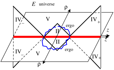
Figure 12: The $\cal{E}$ card diagram consists of eight cards and a singular ergosphere on the horizontal cards V.

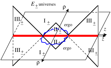
Figure 13: The $\cal{E}_{\pm}$ card diagrams are similar to $\cal{E}$’s. The ${\cal E}_{-}$ universe has a ring singularity atop the ergosphere at $z=0$ (not pictured).

4.1 Interpreting the singularities as connected S-branes

Performing the $\gamma$-flip on the charged Reissner Nordstrom bubble results in the charged S-brane which we call S-RN, which in its parabolic card description is a ‘butterfly’ diagram with two horizontal half-plane cards and four vertical noncompact wedge cards. The $\gamma$-flip and the small-$\sigma$ scaling limit commute, and so one can achieve S-RN as a near-vertex scaling limit of the ${\cal E}$-universes.

We see that the S-RN curvature singularity (and since it is formally the same, the RN curvature singularities) now has an interpretation as an ‘ergosphere’ singularity. (See Appendix B.3, where we discuss the character of such a singularity and also show how the Kerr ‘ring’ singularity can be interpreted as an ergosphere singularity.) By ergosphere singularity, we mean one that can be eliminated via an appropriate inverse Bonnor transformation or appropriate dilatonization and KK lift (see Sec. B.2). Indeed, if one interchanges the roles of $t,\phi$ and inverse Bonnor transforms the negative mass card for the RN black hole, the curvature singularity becomes a nonsingular ergosphere. Unfortunately, $\rho=0$ (where the $\phi$-circle had vanished) becomes singular.

It is not clear how general and useful this idea may be—which familiar and unfamiliar curvature singularities in $D$ dimensions can be easily lifted by an analogous procedure, and what spacetimes result. A generalization of the Bonnor transform or dilatonization procedures should yield interesting results.

In any event, near-vertex scaling limits of the ${\cal E}$ universe towards either $r=r_{+}$ or $r=r_{-}$ give the charged S-Reissner Nordstrom universes with different $M_{\rm RN}$ and $Q_{\rm RN}$ in their parabolic representations. Going down the infinite-proper-distance ‘throat’ towards the vertex means going toward the conformal boundary of ${\bf H}_{2}$ in a particular direction. However, here the two S-branes singularities are connected across the interior of the horizontal card. Note that there is a singularity on the front horizontal card and another on the back horizontal card, just like for S-RN. Just like the singularities of the S-RN, the cards on different cards are not connected. In the case of the ${\cal E}_{-}$ universe, an additional ‘ring’ singularity as a point on the ergosphere singularity complicates the structure.

The factor $\Sigma-2Mr$, which serves as the numerator coefficient of the non-Killing and spatial $x^{4}$ parts of the metric, goes to zero near the singularity which therefore has zero size. The only question is what is the topology of the singularity. From an intuitive viewpoint of a ‘covering surface,’ a time$=$constant slice of RN’s deep interior ($0<r<r_{-}$) can be cut in two (and hence the black hole ‘covered’ by an $S^{2}$), whereas no such $S^{2}$ exists for the Schwarzschild S-brane, and a planar topology surface is necessary to cover the singularity.

Using a given Killing direction for time and approaching the singularity locus using a hypersurface orthogonal coordinate system, the singularity inherits a conformal structure. Here, the ${\cal E}$ or ${\cal E}_{+}$ universes have

$$ds_{2}^{2}\propto{1\over\Sigma^{2}}\Big{(}(dx^{4})^{2}+{\Sigma^{4}\over(\Delta+(M^{2}-a^{2})\sin^{2}\theta)^{3}}\left.\big{(}{dr^{2}\over\Delta}+d\theta^{2}\big{)}\right|_{\rm hypersurface\ constraint}\Big{)}.$$

This is conformally the plane. In two dimensions, all conformal geometries are locally conformally flat, so this construction really only specifies the topology of the singularity. We assume that given this smooth conformal structure, after multiplying by time, we get the same topology as that given by the g-boundary (geodesic parameter space) construction introduced by Geroch [50]. Geroch emphasizes that the topology of the singular boundary of a space is determined by the space’s metric.

The ${\cal E}_{-}$ universe has a ring singularity breaking the ergosphere singularity’s conformal plane into two pieces, and our conformal technique is less appropriate.

Note that we can quotient ${\cal E}_{\pm}$ by ${\mathbb{Z}}_{2}$ in the following way: We can identify the card diagram with a 180-degree rotated version of itself. The universe external to the singularity has no fixed points under this identification. This identifies the two S-brane vertices; there is now one singularity of topology ${\bf R}^{2}$. We are left with one horizontal card, one vertical card to the future, and one vertical card to the past. A conformal squaring of the horizontal card at the origin gives a singly covered card diagram. This quotient is not possible for the ${\cal E}$ universe; one acceleration horizon has a larger length scale than the other.

One can also quotient the ${\cal E}$ and ${\cal E}_{\pm}$ universes by compactifying the $x^{4}$-direction. This is analogous to quotienting the S-RN solution via ${\bf H}_{2}\to{\bf H}_{2}/\Gamma$, for some group $\Gamma$.

Since distances around and near the singularity are vanishingly small, any concomitant shift of time $\phi$ under any of these identification would yield CTCs.

Examining the EM field strength for the ${\cal E}$ universe, we notice the following fact. On the horizontal card (region V of Figs. 4,13), there is an electric field in the $r$ direction, and for large values of $\theta$, $F_{\phi r}=2M/a$ is constant. One can then interpret this as a background electric field which is related to the two-dimensional object lying along the ergosphere singularity. As time passes (we eventually go up the vertical IV_± cards) the electric field eventually goes to zero so this gives support for the interpretation of the S-dihole ${\cal E}$-universe as the creation of a localized two-dimensional unstable object. In contrast, the dihole wave is the formation and decay of a localized fluxbrane, which is a one-dimensional object.

4.2 Scaling limit of simultaneous S-branes to Melvin, flat space

Like the black dihole [51] and dihole wave [12], we can achieve a Melvin scaling limit for some S-dihole universes. The Melvin universe has cylindrical symmetry, with a magnetic field which decays to zero in the transverse direction. The quantity $\Sigma-2Mr$, whose zero locus yields the ergosphere singularity, is the quantity of interest yielding the nontrivial spatial dependence. Both the parameters $M$, $a$, and $\theta-\pi/2$, $\zeta$ must be scaled such that $(\theta-\pi/2)\sim\zeta\to 0$ and $M\zeta\sim a$ (hence $M\gg a$).

The dihole and S-dihole (and dihole wave) are related by analytic continuation, and the Melvin universes which come from the dihole and dihole wave are actually from the same neighborhood of their complexified 4-manifolds. Since the $r\geq r_{+}$ dihole is region I₊, and II₊ is directly adjacent (near $\rho=0$, $z=0$), we must also have a Melvin scaling limit in II₊. For $r\leq r_{-}$, similar remarks apply to I_- and II_-. As part of the ${\cal U}_{\pm}$ universes, II_± scale to

$$ds^{2} = \Big{(}{a^{2}+\rho^{2}\over 4M^{2}}\Big{)}^{2}\Big{(}{4M^{2}\over a^{2}}\Big{)}^{4}\big{(}(dx^{4})^{2}-d\tau^{2}+d\rho^{2}\big{)}+\big{(}{4M^{2}\over a^{2}+\rho^{2}}\big{)}^{2}\rho^{2}d\phi^{2}$$ (39)

$$A = -a\tau dx^{4}/2M^{2}.$$

As part of the ${\cal E}_{\pm}$ universes, we must turn (39) on its side, changing

$$-d\tau^{2}+d\rho^{2}\to d\tau^{2}-d\rho^{2}$$

and going through the $\rho=0$ horizon by $\rho\to i\rho^{\prime}$ to yield a 4-card S-Melvin scaling limit, with an ergosphere singularity at $\rho^{\prime}=a$ on the horizontal cards [52].

There is no corresponding (S-)Melvin scaling limit for regions II or V. The $M\gg a$ requirement makes the ergosphere ellipse in Fig. 5 very wide, so that on the horizontal card V, it becomes infinitely far away from the $\rho=0$ horizon at $\theta=0$. Hence ${\cal U}$ and ${\cal E}_{\pm}$ have no Melvin scaling limit. There is also no Melvin limit for the superextremal S-dihole (Sec. 3.4).

There is also a universe inside the singularity on cards V, and with time-dependent cards II. There is also a scaling limit towards the center vertex of Fig. 5, where the special null lines meet. To the future and past vertices of II, this interior ${\cal E}$-universe becomes flat space in unusual coordinates

$$ds^{2}=(dx^{4})^{2}+{M^{8}(-d\theta^{2}+d\zeta^{2})\over(M^{2}-a^{2})^{3}((\pi/2-\theta)^{2}+(\pi/2-\zeta)^{2})^{3}}+(M^{2}-a^{2})d\phi^{2},\qquad A=2ad\phi.$$

This demonstrates that in the past and future, the spacetime is flat and that the singularity is a transient phenomenon. Picking a sign for each of $\pi/2-\theta$, $\pi/2-\zeta$ (there are four choices) gives us a complete metric $\propto-dx^{+}dx^{-}$ for each wedge card that meets at the vertex. It is clear that special null lines act as ${\cal I}^{\pm}$ here. We have ${\bf R}^{2,1}\times S^{1}$, where the proper circumference of the $S^{1}$ is $2\pi\sqrt{M^{2}-a^{2}}$ and the Wilson line (as approached from Region II) is $4\pi a$.

5 Summary

In this paper we focused on the bubble déjà vu universes labeled as $\cal{U}$ which are a subset of the six subextremal S-dihole universes. These bubble déjà vus represent boundary changing solutions in the sense that the solution time evolves from a charged bubble of nothing with a compactified circle to uncompactified flat space. The three subextremal $\cal{U}$-type universes were nonsingular and had near-vertex scaling limits to the charged Reissner-Nordström bubble. This is the first time a known solution, the charged bubble of nothing, has been associated to a scaling limit of another time dependent solution. We also discussed the extremal $a=M$ solution which was singular and the superextremal $a<M$ solutions which were non-singular. Through a combination of card and Penrose diagrams, we studied the features of the spacetimes and depicted their global structure.

The roles of card, spherical prolate, and affine coordinates have been clarified, as has the location of the ergosphere, ring singularity, special $\rho^{2}=0$ loci, and their mutual intersections (Appendix 3.2.1 contains further details). Dilatonized solutions lift to IIA string theory and M-theory as configurations of D6- and D̄6-branes at real and imaginary coordinate positions. By studying the card diagrams we found an unusual equality relating the bolt structure of black hole horizons to a new bolt-like structure for time dependent S-branes. These relationships in fact are equivalent in the cases we checked to the integrated first law of thermodynamics or the Smarr formula. We believe that is is unlikely that this is a coincidence and it would be interesting to explore this relationship further as it may be useful in better understanding time dependent backgrounds and their excitations. Since it is known how to embed these solutions into string theory it would be worthwhile to pursue whether by analytic continuation we can understand how to count the microstates of time dependent backgrounds. For example bubbles of nothing have an imaginary brane interpretation and a well defined area via our new counting using the Weyl card as a guide. We leave it for the future to be more quantitative and examine if the causal entropy can be attributed to imaginary sources.

One interesting application of these solutions is in tachyon condensation and possible change from branes to flux. It has been recently suggested that a black string can make a transition to a charged bubble of nothing. One question which arose though about this procedure is what happens to the entropy of the black string. It would be interesting to check if entropy can be encoded in bubbles of nothing which would satisfy a version of area entropy relations. It would be fascinating to also explore whether one could interpret the proposed black hole to bubble transitions as the transition of singularities from the real spacetime to imaginary singularities.

Finally we briefly discussed related simultaneous S-branes which we called the $\cal{E}$ universes. These spacetimes had ergosphere singularities, represented the decay of two-dimensional unstable objects, and had a near-vertex limit giving the S-Reissner-Nordström solution. The superextremal S-dihole has a simple card diagram. Physically it shows the creation and decay of an asymptotic conical deficit, and it has an S-charge that is conserved only in a limited sense (on constant-time Weyl slices as we discuss in App. A). This is in contrast with the dihole wave which has a robustly conserved S-charge.

Appendix A Global Properties of Bubble Déjà Vu

A.1 S-charge

For an S-brane solution with electromagnetic field, the magnetic S-charge [3, 10] is defined as the integral of $F$ over a two dimensional surface ${\cal S}$ which is spacelike and transverse to the brane (or Killing) direction. In the absence of sources or singularities and with sufficient decay of fields at infinity, the S-charge is conserved in the sense that it does not depend on ${\cal S}$.

In [12] the S-charge of the dihole wave for $r\geq r_{+}$ was computed in Weyl coordinates over a constant-$\tau$ slice to be $Q_{s}={M\over a}(M+\sqrt{M^{2}+a^{2}})$ and was shown to be conserved. We point out that this charge is very similar to the area of the Kerr horizon and it would interesting to know if it is also subject to something analogous to the area entropy relations. The S-charge along a constant-$t$ slice in BL coordinates can be shown to give the same result. The result for the dihole wave with $r\leq r_{-}$ is the same, up to putting $M\to-M$ in the above formula.

S-dihole (9) has a vector potential

$$A={2aMr\sinh^{2}\theta\over r^{2}-2Mr+a^{2}\cosh^{2}\theta}d\phi.$$

The superextremal $a^{2}>M^{2}$ spacetime has a simple card diagram—it is free of horizons, singularities and special null lines. To compute the S-charge on a BL slice, we fix $r$ and integrate $F_{\theta\phi}$

$$Q_{s}={1\over 4\pi}\int_{0}^{2\pi}d\phi\int_{0}^{\infty}d\theta{\partial\over\partial\theta}\Big{(}{2aMr\sinh^{2}\theta\over r^{2}-2Mr+a^{2}\cosh^{2}\theta}\Big{)}=Mr/a.$$

This is not conserved, and is due to the fact that $F_{r\phi}$ does not decay fast enough; as $\theta\to\infty$ the $drd\phi$ flux integral is $d\Phi_{\infty}={4\pi M\over a}dr$.

Figure 14: Calculation of S-charge on Boyer-Lindquist versus Weyl time slices can lead to different results.

On the other hand, we can compute S-charge for superextremal S-dihole at fixed Weyl time $\tau$. In this case $A|_{\rho=0}=0$ and $A|_{\rho\to\infty}=-2M^{2}/a$ so the S-charge is $Q_{s}=M^{2}/a$. This result is independent of $\tau$ and so superextremal S-dihole has a ‘conserved’ S-charged in a quite limited sense.

The difference between the BL and Weyl S-charges can be seen from looking at the surfaces ${\cal S}$ in Weyl coordinates: The BL constant-$r$ slice asymptotes to a finite, nonzero slope at large values of $\theta$ as shown in Fig. 14. We stress that $r=$ constant slices tend to $i^{0}$ as $\theta\to\infty$.

The S-charges along $r=$ and $\tau=$ constant are equal at $r=M$ ($\tau=0$), which is in a sense the center of the cone of the Einstein-Maxwell waves (this is like a null cone in ${\bf R}^{2,1}$); we could say this is where the solution experiences a ‘bounce,’ but there is no time-symmetry since $M\neq 0$.

The subextremal case ${\cal U}$-universes are less directly amenable to S-charge than the superextremal S-dihole. The noncompact wedges which are regions III_± and IV_± have finite but nonconserved S-charge as we compute along a constant-time (say BL time $r$) slice out to the (null) boundary. However, these surfaces ${\cal S}_{r}$ asymptote to the conformal infinity ${\cal I}^{\pm}$, not to $i^{0}$. One can compactify the noncompact wedge à la Penrose, and the emergent $i^{0}$ has infinite S-charge, being the limit as one runs up ${\cal I}^{-}$.

On the other hand, the compact wedge cards have a clear $i^{0}$ on the card diagram. S-charges are conserved and finite; one evaluates $A_{\phi}$ at $i^{0}$ and subtracts $A_{\phi}$ evaluated anywhere on the $\rho=0$ boundary. Keeping in mind that $\phi\simeq\phi+2\pi$ for ${\cal U}$ and $\phi\simeq\phi+2\pi a^{4}/(M^{2}-a^{2})^{2}$ for ${\cal U}_{\pm}$, the S-charges are $Q_{s}=a$, and $Q_{s}^{\pm}={a^{4}\over(M^{2}-a^{2})^{2}}(a-Mr_{\pm}/a)$. The S-charge suggests that the $i^{0}$ in the upper, middle, and lower cards are disjoint, and helps us conclude the global structure (see Sec. A.3 and Fig. 17).

A.2 A desingularizing change of coordinates

Figure 15: The shown patch for $\alpha$, $\beta$, on the right, fills out three triangles on the $CZ$ diagram, left, for the three cards of the S-dihole ${\cal U}$-universe.

The three vertical cards for the ${\cal U}$-universe, lie on the patches

$$0\leq\rho<{\rm min}(|z-\sqrt{M^{2}-a^{2}}|,|z+\sqrt{M^{2}-a^{2}}|),$$

which are not easily amenable to finding a cross-patch or global description. As the first step to a better global spacetime coordinates, we give a desingularizing transformation, which re-renders the degenerate vertex (where the complex ergosphere locus pierces the vertical cards at $\rho=0$, and where the RN bubble scaling limit is to be found) as a line segment.

One must find equations for orbits as drawn in Fig. 15. The answer has been given implicitly by Penrose’s ideas for compactifying the 1+1 half-plane, using the hyperbolic tangent, and by analytically continuing to achieve the noncompact wedges with the hyperbolic cotangent. In terms of the dimensionless spherical prolate coordinates, the transformation is

$$Z={\alpha(1-\beta^{2})\over 1-\alpha^{2}\beta^{2}},\qquad C=1-{\beta(1-\alpha^{2})\over 1-\alpha^{2}\beta^{2}}.$$

We require $0\leq\beta<1$, and also $\beta<1/|\alpha|$. For fixed $\beta$, an $\alpha$-orbit for $-1/\beta<\alpha<1/\beta$ snakes through all three vertical cards, hitting each vertex with slope $\Delta C/\Delta Z=2\beta/(1+\beta^{2})$. The resulting $\alpha\beta$ coordinate system is not Penrosian in the sense of drawing light cones on the coordinate patch; there is a cross-term. To get the RN scaling limit, near the vertex, $\alpha-1\approx\sigma/2$ (see (12)).

Note then how the degenerate vertices have become the segment $0\leq\beta<1$ for $\alpha=\pm 1$. This coordinate system is not adapted to the full spherical prolate diagram, merely to the three given cards for the ${\cal U}$-universe and their reflections about $C=1$.

If one likes, one can rectangularize the coordinate patch via

$$\alpha_{\rm final}=\tanh^{-1}(\beta\alpha)/\tanh^{-1}(\beta).$$

Then the patch is $0\leq\beta<1$, $-\infty<\alpha_{\rm final}<\infty$.

A.3 Three dimensional diagram for ${\cal U}$ universe

A conjunction of both the Penrose diagram (in $\sigma,x^{4}$) and card diagram (in $\sigma,\eta$) highlights the features of the spacetime, but it would be nice to have a 3-diagram (where only $\phi$ is ignored) to show the global properties of the spacetime, like its topology and the conformal structure at infinity. For the near-vertex limit which is the RN bubble, its fibered dS₂ has the Penrose diagram in Fig. 16(a) and a 3-diagram (ignoring the bubble circle $\phi$) in Fig. 16(b) [17, 18].

Figure 16: (a) The Penrose diagram for dS₂. (b) A 3-diagram of the Witten bubble; the spacetime lies spatially outside dS₂, and is cut into two patches by the parabolic coordinates for dS₂.

For the ${\cal U}$ universe, the 3-diagram is as shown in Fig. 17, where the nondrawn $\phi$-direction closes the spacetime in a warped bubble locus. The bubble has a vertex which is stretched to infinite distance, and serves as $i^{\pm}$ for the lower and upper cards, and part of $i^{0}$ for the middle card. This is the vertex appearing on Fig. 9; in fact, the Penrose diagram of Fig. 9 can be wrapped onto the bubble surface of Fig. 17. S-charge is finite along any curve in the diagram extending from the bubble surface to a point between the lower $i^{0}$ and the upper $i^{0}$, at and beyond which it becomes infinite.

Dashed lines are drawn to indicate the Poincaré horizons for the near-horizon dS₂. These lines must extend as null planes and pierce ${\cal I}$. These piercings must be interpreted as another (spacelike-extended) $i^{0}_{\rm anom}$, with ${\cal I}^{+}$ below it and ${\cal I}^{-}$ above it. This is no conventional $i^{0}$; it serves to separate ${\cal I}^{+}$ from ${\cal I}^{-}$ and represents a breakdown of ${\cal I}$’s smooth conformal structure. The Poincaré horizons hit ${\cal I}$ in a fashion not analogous to Fig. 16.

We argue for the given $i^{0}$’s and $i^{0}_{\rm anom}$’s as follows. From the card diagram, there must be precisely one $i^{0}$ of topology ${\mathbb{R}}$ on the interior of each card. Since the $i^{0}$ on the middle card cannot split, by time-reversal isometry (for say the ${\cal U}_{\pm}$ universes) and by $x^{4}\to-x^{4}$ symmetry it cannot attach to either of the $i^{0}$’s on the upper or lower card, on either side. Lying between the two Poincaré horizons, as $x^{4}\to\pm\infty$ it must approach the bubble vertex. The upper/lower card $i^{0}$’s must lie above/below their Poincaré horizons, and must approach $i^{\pm}$ as shown.

S-charge analysis also implies that the upper/lower $i^{0}$’s cannot meet the interior of $i^{0}_{\rm anom}$’s.

One may object that the given diagram is not Penrosian (causal as drawn, i.e. respecting ${\mathbb{R}}^{2,1}$ light-cones) in that the ${\cal I}^{\pm}$, if they are null cones at $45^{\circ}$, cannot intersect at the Poincaré horizons as depicted. Actually, the 3-metric for the S-dihole is not conformally flat, so no 3-diagram can be Penrosian. This lack of conformal flatness of the 3-metric persists even with $a=0$ or $a=M$. The thing to check is the vanishing of the 3-tensor [53])

$$R_{abc}=R_{ab|c}-R_{ac|b}+{1\over 4}(g_{ac}R_{|b}-g_{ab}R_{|b}),$$

where all quantities are for the 3-manifold and the stroke indicates covariant differentiation. We conclude that the S-dihole’s 3-diagram can only be considered a schematic, and find no further objections to Fig. 17. (The charged Witten bubble’s 3-metric

$$ds_{3}^{2}={dr^{2}\over f(r)}+r^{2}d{\rm dS_{2}}^{2}$$

is conformally flat. The 3-submetric for the Kerr bubble, however is not conformally flat, so the 3-diagram in [18] must also be considered schematic.)

Figure 17: The 3-diagram, analogous to that for the Witten bubble, for the ${\cal U}$-universe. The azimuthal symmetry of the Witten bubble is broken to a Poincaré translation symmetry. There are three disjointed sets of $i^{0}$, and three each of ${\cal I}^{\pm}$. The Poincaré horizons extend as 2-planes in the diagram to pierce null infinity and cause a singularities $i^{0}_{\rm anom}$ in its conformal structure.

Appendix B Characterization of Singularities

Bonnor [31] found how to transform a Weyl-Papapetrou metric to a magnetically charged static Weyl metric. The Bonnor transformation takes the Weyl-Papapetrou metric (17) to the magnetostatic Weyl

$$ds^{2} = -f^{2}dt^{2}+f^{-2}(e^{8\gamma}(d\rho^{2}+dz^{2})+\rho^{2}d\phi^{2}),$$ (40)

$$A = B(\rho,z)d\phi,$$

where $\omega=iB$ and $\omega$ is proportional to a parameter ($a$ in the case of Kerr) which must be analytically continued to make $B$ real.

In this appendix we discuss properties of the Bonnor transorm as they pertain to the Kerr and dihole metrics. The Kerr and Kerr bubble solutions, under Bonnor transform, become the black dihole and dihole wave solutions. Acting on S-Kerr or the double-Killing bubbles of Kerr, the Bonnor for example produces our new solutions which we refered to collectively as S-dihole solutions.

B.1 Generating nontrivial geometries from trivial ones

We have seen how the near-vertex scaling limit of the ${\cal U}$ universe gives us the RN bubble. Turned on its side, this gives us the Reissner-Nordström S-brane (S-RN). This should be the Bonnor transform of a near-vertex scaling limit of Kerr’s double Killing bubble, ${\cal K}_{+}$ for $r\geq r_{+}$. Specifically, we want to zoom in on the north pole of the Kerr horizon, i.e. $\theta=0$ for ${\cal K}_{+}$’s rod, at $z=\sqrt{M^{2}-a^{2}}$, $\rho=0$. Such focusing limits on nonextremal geometries always give flat space, albeit in a strange coordinate system. For ${\cal K}_{+}$’s north pole, flat space is written on the horizontal card $0\leq 2\eta\leq\pi$ as

$$ds^{2} = d\epsilon^{2}+\epsilon^{2}d\eta^{2}-\epsilon^{2}(M^{2}\cos^{2}\eta-a^{2})(dt+a\sin^{2}\eta d\phi/(M^{2}\cos^{2}\eta-a^{2}))^{2}$$

$$+{\epsilon^{2}(M^{2}-a^{2})\cos^{2}\eta\sin^{2}\eta d\phi^{2}\over M^{2}\cos^{2}\eta-a^{2}}.$$

The corresponding instanton ($t\to ix^{5},\,a\to ia$) has a self-dual nut [47] at $\epsilon=0$ for the Killing vector $\partial/\partial x^{5}$.

The point is then that since the Bonnor transform relies on (i) a choice of two Killing directions to put the metric in Weyl-Papapetrou form and (ii) and choice of one of those two Killing directions to be ‘time.’ As this choice is not unique, and we can even have a nontrivial Bonnor transform of flat space. In the present example, the near-north-pole limit of ${\cal K}_{+}$, with its Killing time $t$ and azimuth $\phi$, transforms to give us the S-RN solution in Poincaré/parabolic coordinates [29, 30], where $t\to ix^{5}$ is reduced and $\phi$ becomes the bubble Euclidean circle. Kerr’s ergosphere has become the S-RN singularity.

B.2 Uplifting ergosphere singularities

The ergosphere singularity of a dilatonized version of S-Melvin was found and discussed in [52]. Just as dilatonized Melvin can be obtained by twisting a completely flat KK direction with an azimuthal angle [44], dilatonized S-Melvin can be obtained by twisting a completely flat KK direction with a boost parameter. The ergosphere singularity is then where the twisted KK direction becomes null. On one side of the ergosphere singularity (small $\rho$ on the horizontal card), the twisted KK direction is spacelike whereas on the other side (large $\rho$ on the horizontal card) it is timelike yielding a KK CTC.

Actually, this is a general feature of ergosphere singularities in Einstein-Maxwell-dilaton theory: The singularity occurs where the KK Killing direction goes null. This also occurs in the Bonnor transformation (see Appendix B.3). We wish to emphasize the following connection: The ‘ergosphere,’ where a timelike Killing direction of say Kerr becomes null and switches to spacelike, maps via the Bonnor transformation to an ergosphere singularity of say the S-dihole ${\cal E}_{+}$, where a dilatonized version has a KK circle changing signature. The precise connection is that the Bonnor transformation can be understood from the KK perspective in reducing from five to four dimensions. If we take a magneto-Weyl (MW) solution (40) and dilatonize it with $\alpha=\sqrt{3}$ [35] we get

$$ds_{\rm dil}^{2} = -f^{1/2}dt_{\rm MW}^{2}+f^{-1/2}\big{(}e^{2\gamma}(d\rho^{2}+dz^{2})+\rho^{2}d\phi^{2}\big{)}$$

$$A_{\rm dil} = {1\over 2}Bd\phi$$ (41)

$$e^{2\phi} = f^{\sqrt{3}/2}.$$

Lifting to 5 dimensions [44, 12], we get

$$ds_{\rm 5d}^{2}=f(dx^{5}+Bd\phi)^{2}-dt_{\rm MW}^{2}+f^{-1}\big{(}e^{2\gamma}(d\rho^{2}+dz^{2})+\rho^{2}d\phi^{2}\big{)},$$

and the Killing $t_{\rm MW}$ becomes completely flat. It may be dropped and the resulting 4d solution is a Kerr-type instanton. Upon continuing $x^{5}\to it_{\rm Kerr}$ and $B\to-i\omega$, the $x^{5}$ direction becomes Kerr time. Hence $x^{5}$ and $t_{\rm Kerr}$ change signature on the same complexified locus, the ‘ergosphere.’

For a time-dependent Weyl-Papapetrou geometry, we can add a trivial space direction and then KK reduce along a different space direction, and undilatonize. There is no analytic continuation in this case and this is why S-dihole, as the Bonnor transform of S-Kerr, does not have $a\to ia$ relative to it.

The Bonnor transform is related to $5\to 4$ KK reduction and Weyl dilatonization procedures. These dilatonization procedures will not change spacetimes with simple card diagrams, but will destroy the interesting structure of those card diagrams where the special null line serves as conformal null infinity, such as the ${\cal U}$-type and ${\cal E}$-type universes.

B.3 Character of ergosphere and ring singularities

We give a brief characterization of ergospheres and their Bonnor-transforms, and compare them with the ‘ring’ singularity. The Bonnor transform of ergospheres and ring (i.e. usual curvature) singularities in fact are shown to have identical properties.

Given a $2\times 2$ Killing metric in the Weyl-Papapetrou form (17) with the understanding that $\partial_{t}$ is a distinguished direction for an ensuing Bonnor transformation, we can define its ergosphere locus to be the nonsingular locus where the function $f$ vanishes. Then $\omega$ must have a pole like $f^{-1}$ so that

$$\begin{pmatrix}-f&f\omega\\ f\omega&f^{-1}\rho^{2}-f\omega^{2}\end{pmatrix}\to\begin{pmatrix}0&{\rm finite}\neq 0\\ {\rm finite}\neq 0&{\rm finite}\end{pmatrix},$$

where we have nondegeneracy away from $\rho^{2}=0$. In the interior of a card, from (17) we see that $e^{2\gamma}\sim f$ to keep the coefficient of $d\rho^{2}+dz^{2}$ finite. Thus in the Bonnor-transformed geometry (40) we see that the coefficients of $-dt^{2}$ and $d\rho^{2}+dz^{2}$ vanish like $f^{2}$, the coefficient of $d\phi^{2}$ blows up like $f^{-2}$, and the magnetic potential $A_{\phi}$ blows up like $f^{-1}$. (At the card boundary $\rho=0$, we have seen for the dihole that instead, the ergosphere gives nonsingular extremal black holes which are locally AdS${}_{2}\times S^{2}$.) This characterization of ergosphere singularities will help us to identify them—because upon dilatonization and a KK lift to 5d, they are resolved as noted in the previous subsection..

When the Weyl-Papapetrou geometry is singular, we do not have much to say in general, but we will look at the Bonnor transform of the Kerr ring singularity and find a surprise. There, $f\sim 1/\Sigma$ blows up, and $e^{2\gamma}$ stays finite. Then, the Bonnor-transformed geometry has non-Killing $d\rho^{2}+dz^{2}$ as well as $d\phi^{2}$ vanish like $f^{-2}$ and the $-dt^{2}$ direction blows up like $f^{2}$. Also, one can compute the electric EM-dual potential for the black dihole:

$$A_{t}={2Ma\cos\theta dt\over(r^{2}-a^{2}\cos^{2}\theta)},$$

and this blows up like $f$. (It is not surprising that the electric potential blows up at the curvature singularity of a charged black hole.) Thus the Bonnor transform of a ring singularity is just like that for an ergosphere, but with the roles of $\phi$ and $t$ exchanged. It them seems possible that $\Sigma=0$ could be made nonsingular with the right inverse transform. In the present dihole case, the locus intersects the real spacetime at a vertex point where it is algebraically singular, and also is a subset of the ergosphere singularity. Unfortunately there are no immediately new nonsingular geometries from this idea.

Appendix C Dihole fluxbrane waves

We review the dihole fluxbrane wave solution of [12]. It is gotten from the dihole (8) by sending $t\to ix^{4}$, $\theta\to\pi/2+i\theta$. Then $\Sigma=r^{2}+a^{2}\sinh^{2}\theta$, and shifting $A_{\phi}$ to remove the Dirac string, the solution is

$$ds^{2} = \big{(}1-\frac{2Mr}{\Sigma}\big{)}^{2}\Big{(}(dx^{4})^{2}+\frac{\Sigma^{4}}{(\Delta+(a^{2}+M^{2})\cosh^{2}\theta)^{3}}\big{(}\frac{dr^{2}}{\Delta}-d\theta^{2}\big{)}\Big{)}+\frac{\Delta\cosh^{2}\theta}{(1-\frac{2Mr}{\Sigma})^{2}}d\phi^{2}$$

$$A = \Big{(}\frac{2aMr\cosh^{2}\theta}{\Delta+a^{2}\cosh^{2}\theta}-{2Mr_{+}\over a}\Big{)}d\phi\ .$$ (42)

Periodically identifying $\phi\simeq\phi+2\pi a^{4}/(M^{2}+a^{2})^{2}$ eliminates the conical singularity at $r=r_{+}$. The analytic continuation $\theta\to\pi/2+i\theta$ is equivalent to $C\to iS$, where $S=\sinh\zeta$ and $S=0$ is a symmetric line (just like $C=0$ was a symmetric line) but there is no other distinguished $S$. We draw a spherical prolate diagram (Fig. 18). The dihole wave occupies region I, where time points right.

Figure 18: The spherical prolate diagram for the dihole wave (region I). Positive $S=\sinh\theta$ (time) points to the right.

In Weyl coordinates, one obtains the dihole wave by $z\to i\tau$, $t\to ix^{4}$. The card diagram is a vertical half-plane $\rho\geq 0$, $-\infty<\tau<\infty$. The sources (the extremal black hole horizons, which appear as points in Weyl coordinates) are located at $\rho=0$ and $\tau=\pm i\sqrt{M^{2}+a^{2}}$. These are interpreted as the intersection of $\rho^{2}=0$ with the nonsingular ergosphere hypersurface $\Sigma-2Mr=0$ (see Appendix 3.2.1).

The continuation to get the dihole wave is very similar to that to get the Kerr $\pi/2$-bubble [18], which is $t\to ix^{4}$, $\theta\to\pi/2+i\theta$, $a\to ia$; there is then a twisted circle closing at $r=r_{+}$. We can think of the dihole wave as the Bonnor transform of the Kerr bubble (there is no relative $a\to ia$ between them, since the associated 5d Killing submetrics have signature $+++$; see Sec. B.2).

Further discussion of the wave-like character of this solution, the asymptotic fall-off on a null line on the card diagram, scaling limits of the fluxbrane wave including the Melvin universe and the cone can be found in Ref. [29].

Appendix D S-brane in Panleve coordinates

Like the dihole wave fall off, we can also examine the S-Schwarzschild solution

$$ds^{2}_{\rm S-Schwarz}=(1-\frac{2M}{t})dz^{2}-\frac{dt^{2}}{1-2M/t}+t^{2}d{\bf H}^{2}_{2}$$ (43)

and our approach will be to examine the physical properties of this solution and evaluate the S-brane in a different coordinate patch. The main question is what does the parameter $M$ represent. In the case of the black hole this represents the mass or energy of the black hole due to a massive source. Now let us examine the Wick rotation process from the black hole to the S-brane. This changes the time direction to a spatial direction $z$ and as a consequence the energy of the original black hole is now interpreted not as an energy but as a pressure source.

If we add an electric charge, $Q$, to the black hole then there is a stress tensor for the spacetime with

$$T_{\mu\nu} = \frac{1}{4\pi}(F_{\mu\gamma}F_{\nu}^{\gamma}-\frac{1}{4}g_{\mu\nu}F_{\rho\sigma}F^{\rho\sigma})$$ (44)

$$T_{tt} = (Q^{2}/8\pi r^{4})(1-2M/r+Q^{2}/r^{2})\ .$$ (45)

Now let us examine the wick rotation process from the black hole to the S-brane which changes the time direction to a spatial direction $t\to iz$ and the radial direction to a time direction $r\to i\tau$. Therefore the energy of the original black hole is now interpreted not as an energy but as a pressure $T_{zz}=(Q^{2}/8\pi\tau^{2})(1-2M/\tau-Q^{2}/\tau^{2})$. The pressure is clearly identified in the case of the electromagnetic contribution to the S-brane and likewise the same should hold for the uncharged S-brane using an ADM type of definition of the pressure. Clearly the pressure should be and is positive for consistency if we want the $z-$direction to contract. A negative parameter $M$ should then correspond to negative pressure and this is exactly in accordance with the cosmological use of S-brane solutions for cosmology. The parameter $M$ we then interpret as a pressure of the S-Schwarzschild solution. In general one could call an S-brane a “pressure”-brane.

We next use the Schwarzschild Panleve coordinate which foliates the spacetime into flat three dimensional slices at every point in time

$$ds^{2}=-(1-\frac{2M}{r})dt^{2}+2\sqrt{\frac{2M}{r}}drdt+dr^{2}+r^{2}d\Omega^{2}_{2}\ .$$ (46)

Performing the usual Wick rotation in this coordinate system gives the S-brane

$$ds^{2}=(1-\frac{2M}{t})dz^{2}+2\sqrt{\frac{2M}{t}}dtdz-dt^{2}+t^{2}dH^{2}_{2}\ .$$ (47)

Further transforming this Milne coordinate to the usual slicing of Minkowski gives

$$(1-\frac{2M}{\sqrt{T^{2}-R^{2}}})dz^{2}-2\sqrt{\frac{2M}{\sqrt{T^{2}-R^{2}}}}dz\frac{T\ dT-R\ dR}{\sqrt{T^{2}-R^{2}}}-dT^{2}+dR^{2}+R^{2}d\phi^{2}$$ (48)

and we see that for fixed $z$ coordinate values we get three dimensional Minkowski space. The evolution of this spacetime is a mixture of ingoing and outgoing waves centered along $T=\pm R$ which hit/emit from a timelike singularity and spread out in the $z$-direction; the singularity is null in the $T,R$-directions but has a timelike component coming from the z-direction. Travel purely in the radial direction gives flat space. The null singularity however is to be expected any time there is a spacelike singularity source at $z=0$ and the horizon at $t_{0}$ is the relativistic effect.

The $z$-direction represents the extension of the S-brane although in this coordinate system it is clear that there is no linear mass in the system along the $z$-direction unless the angular coordinate $\phi$ has a conical deficit corresponding to an orbifold of the original hyperbolic slicing. However this linear direction gets squeezed by the pressure of the system caused by the mixture of traveling momentum. What is unusual however is that there is no asymptotic region $R\gg T$ where we can see the conical string since we are bounded by the singularity; the conical singularity is only visible locally. In this sense this solution appears as a singular birth and death of a universe.

References

- [1]
- [2] A. Sen, “Non-BPS states and branes in string theory,” arXiv:hep-th/9904207.
- [3] M. Gutperle and A. Strominger, “Spacelike branes,” JHEP 0204, 018 (2002) [arXiv:hep-th/0202210].
- [4] A. Sen, “Rolling Tachyon,” JHEP 0204, 048 (2002), [arXiv:hep-th/0203211]; “Tachyon Matter,” JHEP 0207, 065 (2002), [arXiv:hep-th/0203265]; “Field Theory of Tachyon Matter,” Mod. Phys. Lett. A17, 1797 (2002), [arXiv:hep-th/0204143]; “Time Evolution in Open String Theory,” JHEP 0210, 003 (2002), [arXiv:hep-th/0207105].
- [5] A. Sen, “Tachyon dynamics in open string theory,” arXiv:hep-th/0410103.
- [6] C. M. Chen, D. V. Gal’tsov and M. Gutperle, “S-brane solutions in supergravity theories,” Phys. Rev. D 66, 024043 (2002) [arXiv:hep-th/0204071].
- [7] M. Kruczenski, R. C. Myers and A. W. Peet, “Supergravity S-branes,” JHEP 0205, 039 (2002) [arXiv:hep-th/0204144].
- [8] N. Ohta, “Intersection rules for S-branes,” Phys. Lett. B 558 (2003) 213 [arXiv:hep-th/0301095].
-
[9]
-
J. E. Wang, “Spacelike and time dependent branes from DBI,” JHEP 0210, 037 (2002) [arXiv:hep-th/0207089],
-
C. P. Burgess, F. Quevedo, S. J. Rey, G. Tasinato and I. Zavala, “Cosmological spacetimes from negative tension brane backgrounds,” JHEP 0210, 028 (2002) [arXiv:hep-th/0207104].
-
- [10] A. Maloney, A. Strominger and X. Yin, “S-brane thermodynamics,” JHEP 0310, 048 (2003) [arXiv:hep-th/0302146].
- [11] D. Gaiotto, N. Itzhaki and L. Rastelli, “Closed strings as imaginary D-branes,” Nucl. Phys. B 688, 70 (2004) [arXiv:hep-th/0304192].
- [12] G. C. Jones, A. Maloney and A. Strominger, “Non-singular solutions for S-branes,” Phys. Rev. D 69, 126008 (2004) [arXiv:hep-th/0403050].
- [13] J. E. Wang, “Twisting S-branes,” JHEP 0405, 066 (2004) [arXiv:hep-th/0403094].
- [14] G. Tasinato, I. Zavala, C. P. Burgess and F. Quevedo, “Regular S-brane backgrounds,” JHEP 0404, 038 (2004) [arXiv:hep-th/0403156].
- [15] H. Lü and J. F. Vázquez-Poritz, “Non-singular twisted S-branes from rotating branes,” JHEP 0407, 050 (2004) [arXiv:hep-th/0403248].
- [16] K. Behrndt and S. Forste, “String Kaluza-Klein Cosmology,” Nucl. Phys B430 (1994) 441 [arXiv:hep-th/9403179].
- [17] E. Witten, “Instability Of The Kaluza-Klein Vacuum,” Nucl. Phys. B 195, 481 (1982).
- [18] O. Aharony, M. Fabinger, G. T. Horowitz and E. Silverstein, “Clean time-dependent string backgrounds from bubble baths,” JHEP 0207, 007 (2002) [arXiv:hep-th/0204158].
- [19] D. Birmingham and M. Rinaldi, “Bubbles in anti-de Sitter space,” Phys. Lett. B 544, 316 (2002) [arXiv: hep-th/0205246].
- [20] V. Balasubramanian and S. F. Ross, “The dual of nothing,” Phys. Rev. D 66, 086002 (2002) [arXiv: hep-th/0205290].
- [21] A.M. Ghezelbash and R.B. Mann, “Nutty bubbles,” JHEP 0209, 045 (2002) [arXiv: hep-th/0207123].
- [22] A.M. Ghezelbash, R.B. Mann, “Kerr-AdS Bubble Spacetimes and Time-Dependent AdS/CFT Correspondence,” Mod. Phys. Lett. A19 (2004) 1585 [arXiv: hep-th/0210046].
- [23] D. Astefanesei and G. C. Jones, “S-branes and (anti-)bubbles in (A)dS space,” JHEP 0506, 037 (2005) [arXiv: hep-th/0502162].
- [24] D. Astefanesei, Robert B. Mann and Cristian Stelea, “Nuttier bubbles,” JHEP 0601, 043 (2006) [arXiv: hep-th/0508162 ].
- [25] F. R. Tangherlini, Nuovo Cimento 27, 636 (1963).
- [26] G. T. Horowitz, “Tachyon condensation and black strings,” JHEP 0508, 091 (2005) [arXiv:hep-th/0506166].
- [27] R. Rohm, “Spontaneous Supersymmetry Breaking In Supersymmetric String Theories,” Nucl. Phys. B 237, 553 (1984).
- [28] A. Adams, X. Liu, J. McGreevy, A. Saltman, Eva Silverstein, “Things Fall Apart: Topology change from Winding Tachyons,” JHEP 0510, 033 (2005) [arXiv:hep-th/0502021].
- [29] G. C. Jones and J. E. Wang, “Weyl card diagrams and new S-brane solutions of gravity,” arXiv:hep-th/0409070.
- [30] G. C. Jones and J. E. Wang, “Weyl card diagrams,” Phys. Rev. D 71, 124019 (2005) [arXiv:hep-th/0506023].
- [31] W. B. Bonnor, “An Exact Solution of the Einstein-Maxwell Equations Referring to a Magnetic Dipole,” Zeitschrift für Physik 190, 444 (1966).
- [32] S. Chandrasekhar and B. C. Xanthopoulos, “Two Black Holes Attached To Strings,” Proc. Roy. Soc. Lond. A 423, 387 (1989).
- [33] R. Emparan, “Black diholes,” Phys. Rev. D 61, 104009 (2000) [arXiv:hep-th/9906160].
- [34] H. Stephani, D. Kramer, M. MacCallum, C. Hoenselaers, E. Herlt, Exact Solutions of Einstein’s Field Equations, 2nd ed., Cambridge University Press (2003).
- [35] R. Emparan and E. Teo, “Macroscopic and microscopic description of black diholes,” Nucl. Phys. B 610, 190 (2001) [arXiv:hep-th/0104206].
- [36] W. B. Bonnor, “The Sources of the Vacuum -Metric,” Gen. Rel. Grav. 15 (6) 535 (1983).
- [37] T. Harmark, “Stationary and axisymmetric solutions of higher-dimensional general relativity,” Phys. Rev. D 70, 124002 (2004) [arXiv:hep-th/0408141].
-
[38]
-
J. Bičák and V. Pravda, “Spinning C metric: Radiative space-time with accelerating, rotating black holes,” Phys. Rev. D 60, 044004 (1999) [arXiv: gr-qc/9902075];
-
V. Pravda and A. Pravdová, “Boost rotation symmetric space-times: Review,” Czech. J. Phys. 50, 333 (2000) [arXiv: gr-qc/0003067].
-
- [39] J. Stewart, Advanced General Relativity (Cambridge Monographs on Mathematical Physics).
- [40] G. C. Jones, Time-Dependent Solutions of Gravity, Harvard University thesis (2006) available at http://www.physics.harvard.edu/Thesespdf/Jones.pdf.
-
[41]
-
D. Klemm, V. Moretti and L. Vanzo, “Rotating topological black holes,” Phys. Rev. D 57, 6127 (1998) [Erratum-ibid. D 60, 109902 (1999)] [arXiv: gr-qc/9710123];
-
D. Klemm, “Rotating black branes wrapped on Einstein spaces,” JHEP 9811, 019 (1998) [arXiv: hep-th/9811126].
-
- [42] A. Papapetrou, “Eine rotationssymmetrische Lsung in der allgemeinen Relativitatstheorie,” Ann. Physik 12 (1953) 309; “Champs gravitationnels stationnaires a symetrie axiale,” Ann. Inst. H. Poincaré A 4 (1966) 83.
- [43] T. Harmark and P. Olesen, “On the structure of stationary and axisymmetric metrics,” arXiv:hep-th/0508208.
- [44] F. Dowker, J. P. Gauntlett, G. W. Gibbons and G. T. Horowitz, “The Decay of magnetic fields in Kaluza-Klein theory,” Phys. Rev. D 52, 6929 (1995) [arXiv:hep-th/9507143].
- [45] P. K. Townsend, “The eleven-dimensional supermembrane revisited,” Phys. Lett. B 350, 184 (1995) [arXiv:hep-th/9501068].
- [46] P. K. Townsend, “P-brane democracy,” arXiv:hep-th/9507048.
- [47] G. W. Gibbons and S. W. Hawking, “Classification Of Gravitational Instanton Symmetries,” Commun. Math. Phys. 66, 291 (1979).
- [48] G. C. Jones and J. E. Wang, “S-Kerr Solutions and a New Instanton,” in preparation.
- [49] L. Smarr, “Mass Formula for Kerr Black Holes,” Phys. Rev. Lett. 30, 71 (1973). Erratum, 30, 521 (1973).
- [50] R. Geroch, “Local Characterization of Singularities in General Relativity,” J. Math. Phys. 9, 450 (1968).
- [51] R. Emparan and M. Gutperle, “From p-branes to fluxbranes and back,” JHEP 0112, 023 (2001) [arXiv:hep-th/0111177].
- [52] L. Cornalba and M. S. Costa, “A new cosmological scenario in string theory,” Phys. Rev. D 66, 066001 (2002) [arXiv:hep-th/0203031].
- [53] C. W. Misner, K. S. Thorne, and J. A. Wheeler, Gravitation, W. H. Freeman & Co. (1973).
- [54] H. Weyl, “The theory of gravitation,” Ann. Phys. (Leipzig) 54, 117 (1917).
- [55] S. Fairhurst and B. Krishnan, “Distorted black holes with charge,” Int. J. Mod. Phys. D 10, 691 (2001) [arXiv:gr-qc/0010088].