Matrix Models and QCD with Chemical Potential

Abstract

The Random Matrix Model approach to Quantum Chromodynamics (QCD) with non-vanishing chemical potential is reviewed. The general concept using global symmetries is introduced, as well as its relation to field theory, the so-called epsilon regime of chiral Perturbation Theory ($\epsilon\chi$PT). Two types of Matrix Model results are distinguished: phenomenological applications leading to phase diagrams, and an exact limit of the QCD Dirac operator spectrum matching with $\epsilon\chi$PT. All known analytic results for the spectrum of complex and symplectic Matrix Models with chemical potential are summarised for the symmetry classes of ordinary and adjoint QCD, respectively. These include correlation functions of Dirac operator eigenvalues in the complex plane for real chemical potential, and in the real plane for imaginary isospin chemical potential. Comparisons of these predictions to recent Lattice simulations are also discussed.

1 Introduction

In the phase where chiral symmetry is broken and quarks and gluons are confined Quantum Chromodynamics (QCD) is strongly coupled and perturbation theory breaks down. Several methods alow to study this situation from first principles. In an effective field theory approach only the lowest degrees of freedom are taken into account, such as the pseudo Goldstone bosons in chiral Pertubation Theory ($\chi$PT). Second, in Lattice Gauge Theory (LGT) QCD is studied on a Euclidean space-time lattice. At zero baryon chemical potential $\mu=0$ LGT has been very successful, e.g. in describing the particle spectrum or the chiral phase transition. Turning on $\mu$ in the phase diagram, LGT faces the so-called sign problem: the action becomes complex in general. This invalidates the usual method to weight configurations by their Boltzmann factor, as it ceases to be a real positive quantity.

In this article we will study a simple model called chiral Random Matrix Model (MM) in order to understand some aspects of this problem. This includes insights into chiral symmetry breaking at non-zero chemical potential, and quantitative aspects of the Dirac operator spectrum close to zero momentum, illuminating the interplay between LGT and $\chi$PT. MMs can be mapped to field theory in a particular limit called the epsilon regime or $\epsilon\chi$PT. Clearly QCD is not only a MM, and we will cover aspects dictated by global symmetries alone. Also our MM does not solve the sign problem on the Lattice, but it provides a model that can be exactly solved despite this problem, and that offers quantitative predictions for the Lattice. The three types of real, complex and symplectic chiral MMs match with the classification of gauge theories in general (including QCD) into 3 classes, displaying different ways or the absence of the sign problem.

To start let us briefly summarise what has been achieved for MMs of QCD at zero chemical potential since their introduction in [1]. An excellent review describing its concepts and success can be found in [2]. The introduction of MMs as a tool to study complicated physical systems by means of symmetry predates QCD substantially, going back to Dyson and Wigner in the late 1950 and early 1960. Initially developed for heavy nuclei MMs have today found applications in most fields of physics (and other sciences), as reviewed in [3]. The first MM for the Dirac spectrum of QCD was written down and solved in [1], including all quenched and massless eigenvalue correlation functions for the MM Dirac operator eigenvalues. It became apparent that the 3 fold classification of Dirac operators for different field theories according to charge and complex conjugation symmetry [4] exactly coincides with the 3 possible chiral symmetry breaking patterns [5]. The corresponding 3 MMs are called chiral ensembles, having real, complex and quaternion real matrix elements. All eigenvalue correlation functions for these 3 chiral MMs ensembles were consecutively computed, including an arbitrary number of massive quark flavours $N_{f}$ [1, 8, 9, 10, 11, 12, 13], and individual eigenvalue distributions [14, 10].

The equivalence of such MMs to $\epsilon\chi$PT was first realised on the level of partition functions [1, 15], leading to identical sum-rules for the Dirac operator [16, 17]. As explained by Gasser and Leutwyler [18] the $\epsilon\chi$PT regime also called microscopic domain is reached, when the zero-momentum Goldstone modes completely dominate the partition function, decoupling from Gaussian propagating modes.

The MM density [19] and density-density [20] correlations were shown to coincide with those derived from $\epsilon\chi$PT alone, and consequently the individual eigenvalue distributions to leading order [21]. Note that so far no higher density correlations, nor density correlations in symmetry classes other than QCD have been computed from $\epsilon\chi$PT.

Furthermore it was understood precisely when the MM-$\epsilon\chi$PT correspondence breaks down, at the so-called Thouless energy [22], making the MM approximation transparent. Even when going beyond the MM regime its techniques have been useful to compute expectation values of vector and axial vector currents, see [23] and references therein.

Below the Thouless energy MMs give precise analytic predictions for the low Dirac operator eigenvalues lying inside the $\epsilon$-regime, as a function of quark masses and gauge field topology, for each of the 3 symmetry classes. Such quantitative predictions have been extensively checked in all 3 classes, in quenched and unquenched simulations. First tests were done using staggered fermions, giving confirmation in all 3 symmetry classes [24] in the sector of topological charge $\nu=0$. For staggered fermions care has to be taken compared to the global symmetry in the continuum in 2 of the 3 classes.

The predictive power of MMs has gained even more relevance in the important development of chiral fermions, that possess an exact Lattice chiral symmetry and well defined topology away from the continuum (see [25] for a review). Here MMs have been used to test such algorithms at fixed gauge field topology, being confirmed for all 3 classes by various groups [26]. Subsequently staggered simulations have been improved, also showing the correct topology dependence as overlap fermions [27].

In this article we will try to go through the same steps for MMs with non-zero chemical potential, and compare the analytical prediction available for 2 of the 3 classes to Lattice data whenever possible. Very recently a review on the same topic appeared [28], focusing more on the relation to $\epsilon\chi$PT than the MM concepts, its solution and comparison to LGT covered here.

In order to emphasise the limitations of our approach let us recall some important questions of LGT at finite density and temperature $T$. One of the purposes underlying Lattice simulations is to better understand the restoration of chiral symmetry, going hand in hand with deconfinement for QCD. Major experiments such as RHIC as well as the transition in the early universe happen at very small $\mu$ close to the temperature axis. Here several techniques have been applied to avoid the sign or complex action problem, where we refer to [29] for a review and [30] for recent developments. Physical questions as for the free energy, pressure, equation of state, screening mass or string tension have been addressed, and the dependence on the number of flavours and quark masses is being tested (see [31] for a review and references). However, none of these techniques actually solves the sign problem. For that reason the phase diagram far away from the $T$-axis is still current subject of debate [32].

Our simple MM cannot give answers to these physical questions, despite providing a qualitative (flavour independent) phase diagram for QCD. The domain of our MM solution is at small or zero $T$ and small to moderate $\mu$. Its analytical predictions there can serve as a testing ground, both in the presence or absence of the sign problem. It also can tell us in which region simulations are doable at finite volume and when the sign problem hits in, as reviewed in [28]. Because of this situation so far we can only provide evidence for MM predictions by comparing to quenched Lattice QCD, and to unquenched LGTs not suffering from the sign problem.

Several topics using MMs at finite $\mu$ are not covered in this review. In section 3 we review only aspects of the phase diagram for QCD. Similar results exist for two colours [33] as well, and for a discussion of the chiral Lagrangian with chemical potential for two colours and the adjoint representation we refer to [34]. The phase diagram of QCD can also be analysed using the complex zeros of the partition function, where we refer to recent [35] as well as previous work [36]. Recently the phase of the fermion determinant has been computed [37], which can be tested in Lattice simulations. In addition to chemical potential and temperature also colour degrees of freedom can be taken into account in MMs [38] in order to model single-gluon exchanges, or the symmetries of the staggered operator can be added [39]. However, these additions typically destroy the exact analytical solvability. Last but not least a factorisation method has been advocated by the authors of [40]. It uses MMs as a toy model in order to tackle the sign problem in Lattice simulations. As mentioned earlier MMs enjoy many different applications in Physics. For applications of MMs with complex eigenvalues in other areas we refer to the review [41].

This article is organised as follows. In the next section 2 we explain the concept of our MM approach including a symmetry classification and its relation to $\epsilon\chi$PT. After a brief view on the resulting phase diagrams in section 3, we turn to the relation between Dirac operator eigenvalues and chiral symmetry breaking in section 4. Here we summarise what is know for complex eigenvalue correlation functions in the class containing QCD, and confront with quenched lattice results. Section 5 contains all results for symplectic MMs corresponding to field theories with fermions in the adjoint representation. Here we compare to unquenched Lattice results. In section 6 we present the solution of a MM for the QCD class with imaginary isospin chemical potential where unquenched simulations are straightforward. Conclusions and an outlook are given in section 7.

2 Concept of Matrix Models at Finite $\mu$

2.1 Global symmetries

The general strategy in applying Matrix Models to Physics is to replace a complicated operator by a random matrix with the same global symmetries, trying to gain some information on its spectrum. In 1993 Shuryak and Verbaarschot applied this idea for the first time to the Dirac operator $\hbox to0.0pt{ $\,\raisebox{0.6458pt}{/}\hss$}D$ in QCD [1], which was then extended to QCD with chemical potential by Stephanov [42]:

$$\hbox to0.0pt{ $\,\raisebox{0.6458pt}{/}\hss$}D(\mu)\equiv\hbox to0.0pt{ $\,\raisebox{0.6458pt}{/}\hss$}D+\mu\gamma_{0}\ \longrightarrow\left(\begin{array}[]{cc}0&\Phi+1\!|\,\mu\\ -\Phi^{\dagger}+1\!|\,\mu&0\\ \end{array}\right)\ .$$ (2.1)

The matrix $\Phi$ has constant, that is space-time independent matrix elements, typically with identical Gaussian distributions and hence its name random. Here we have used already 2 global symmetries: in the continuum chiral symmetry implies that $\{\hbox to0.0pt{ $\,\raisebox{0.6458pt}{/}\hss$}D(\mu),\gamma_{5}\}=0$, leading to an off-diagonal block structure. Second, we have used that the Euclidean Dirac operator is anti-hermitian at zero chemical potential, and that $\mu\gamma_{0}$ is hermitian.

The average over the gauge fields of the Yang-Mills action is replaced by a random matrix average,

$$\exp[-S_{gauge}]\ \longrightarrow\ \exp[-\sigma^{2}\mbox{Tr}\ \Phi^{\dagger}\Phi]\ ,$$ (2.2)

when computing observables. The inverse variance $\sigma^{2}$ in the Matrix Model is to be fixed later. Using a lattice regularisation in a finite volume $V$ the Dirac matrix becomes finite dimensional, and we thus can choose the random matrix $\Phi$ of dimension $N\times(N+\nu)$. Here we have furthermore restricted ourselves to a sector of fixed topology $\nu$, or through the index theorem to a fixed number of zero modes of $\hbox to0.0pt{ $\,\raisebox{0.6458pt}{/}\hss$}D$. Its eigenvalues are defined as

$$\hbox to0.0pt{ $\,\raisebox{0.6458pt}{/}\hss$}D(\mu)\varphi_{k}\ =\ iz_{k}\varphi_{k}\ ,\ \ k=1,\ldots,V\ \ (\mu=0\Rightarrow z_{k}\in\mathbb{R})\ .$$ (2.3)

For zero $\mu$ they lie on the imaginary axis, whereas for nonzero $\mu$ the operator $\hbox to0.0pt{ $\,\raisebox{0.6458pt}{/}\hss$}D(\mu)$ has complex eigenvalues in general, being a complex non-Hermitian operator. The large-$N$ limit in the matrix size thus corresponds to the thermodynamic limit $\lim 2N\sim V\to\infty$, keeping the size of the gauge group $N_{C}$ fixed.

$SU({2})$ fund.	$SU({N_{C}\geq 3}),\ U(1)$ fund.	$SU({N_{C}})$ adjoint
$\hbox to0.0pt{ $\,\raisebox{0.6458pt}{/}\hss$}D(\mu)=\left(\begin{array}[]{cc}0&\Phi+1\!|\mu\\ -\Phi^{T}+1\!|\mu\\ \end{array}\right)$	$\left(\begin{array}[]{cc}0&\Phi+1\!|\mu\\ -\Phi^{\dagger}+1\!|\mu&0\\ \end{array}\right)$	$\left(\begin{array}[]{cc}0&\Phi+1\!|\mu\\ -\Phi^{\dagger}+1\!|\mu&0\\ \end{array}\right)$
$\Phi_{ij}$$\in\ \mathbb{R}$,  $\beta_{D}=1$	$\Phi_{ij}$$\in\ \mathbb{C}$ , $\beta_{D}=2$	$\Phi_{ij}$$\in$ real $\mathbb{H}$ , $\beta_{D}=4$
as $[C\sigma_{2}K,\hbox to0.0pt{ $\,\raisebox{0.6458pt}{/}\hss$}D]=0$		as $[CK,\hbox to0.0pt{ $\,\raisebox{0.6458pt}{/}\hss$}D]=0$
$\exists$ finite fraction $z_{k}\in\mathbb{R}$		$\forall k:$ $z_{k}\notin\mathbb{R},i\mathbb{R}$
$SU({N_{C}})$ adjoint staggered	$SU({N_{C}\geq 3}),\ U(1)$ fund.	$SU({2})$ fund. staggered
	staggered

Table 1: Table of global symmetry classes.

What are the matrix elements of $\Phi$? It turns out that they can be further restricted by symmetry and fall into 3 different classes. According to the choice of gauge group and its representation it was shown for gauge groups $SU(N_{C})$ at $\mu=0$ [4] and at $\mu\neq 0$ [34] that for either two colours $N_{C}=2$ or the adjoint representation an anti-unitary symmetry allows to choose the matrix elements $\Phi_{ij}$ to be real or quaternion real, respectively. For the class with $SU(N_{C}\geq 3)$ in the fundamental representation containing QCD no such symmetry exists, and the matrix elements are complex. These are the global symmetries that the random matrices and the exact Dirac operators share, as shown in the table 1. This classification can of course be extended to any gauge groups having a real, complex or pseudo-real representations, and we have added $U(1)$ to the table.

The anti-unitary symmetry in the real and pseudo-real case is provided by a product of the charge $C$ and complex conjugation matrix $K$, and a Pauli matrix $\sigma_{2}$ for $SU(2)$ [4, 34]. We have introduced the Dyson index $\beta_{D}$ to label the number of independent degrees of freedom per matrix element of $\Phi$. In the class $\beta_{D}=1$ the non-symmetric, real matrix $\hbox to0.0pt{ $\,\raisebox{0.6458pt}{/}\hss$}D(\mu\neq 0)$ has a real secular equation. Hence it can have real eigenvalues in addition to complex eigenvalues occuring in conjugated pairs. For that reason this class has a real $\det[\hbox to0.0pt{ $\,\raisebox{0.6458pt}{/}\hss$}D(\mu)]$ which is not necessarily positive. This sign problem is thus reduced from a phase to a fluctuating sign. For an even number of two-fold degenerate flavours the product of all determinants remains positive and has no sign problem. For $\beta_{D}=4$ the determinant $\det[\hbox to0.0pt{ $\,\raisebox{0.6458pt}{/}\hss$}D(\mu)]$ is alway positive, as the eigenvalues of a real quaternion matrix occur in complex conjugated pairs [44].

Notice that for discretised Dirac operators on a Lattice their global symmetries may change: when using staggered fermions the symmetry classes $\beta_{D}=1$ and 4 have to be interchanged [45]. On the other hand Wilson type Dirac operators are in the same symmetry class as the continuum. So far the transition from the discrete to the continuum symmetry class has not been observed for staggered fermions in the Dirac spectrum.

	$\mu=m=0$	$\mu\neq 0,\ m\geq 0$
$\beta_{D}=1$	$SU(2N_{f})\to Sp(2N_{f})$	$SU(N_{f})_{L}\times SU(N_{f})_{R}\to$	$Sp(N_{f})_{L}\times Sp(N_{f})_{R}$
		$\to$	$Sp(N_{f})_{V}$ for $m\neq 0$
$\beta_{D}=2$	$SU(N_{f})_{L}\times SU(N_{f})_{R}\to SU(N_{f})_{V}$	$SU(N_{f})_{L}\times SU(N_{f})_{R}\to$	$SU(N_{f})_{V}$
$\beta_{D}=4$	$SU(2N_{f})\to SO(2N_{f})$	$SU(N_{f})_{L}\times SU(N_{f})_{R}\to$	$SO(N_{f})_{L}\times SO(N_{f})_{R}$
		$\to$	$SO(N_{f})_{V}$ for $m\neq 0$

Table 2: Table of spontaneous (left) and explicit (right) chiral symmetry breaking patterns.

It turns out that the classification into 3 groups exactly corresponds the 3 possible patterns of spontaneous chiral symmetry breaking introduced by Peskin [5], where a maximal breaking is assumed. Here we have dropped both the vector $U_{V}(1)$ and axial vector $U_{A}(1)$ factor as they are not affected by the spontaneous breaking. The case of symmetry breaking in 2 dimensions is special, and we refer to [46] for an exhaustive treatment of the Schwinger model and its relation to MMs.

The mass term in $\chi$PT (see eq. (2.10)) of course explicitly breaks chiral symmetry. At $\mu=0$ the patterns are the same as for spontaneous breaking in all 3 classes, see table 2. A nonzero $\mu$-term also explicitly breaks chiral symmetry, and the breaking patters differs from the spontaneous one for $\beta_{D}=1,4$ as discussed in [34], both for $m=0$ and $m\neq 0$. There is a competition for the vacuum aligning to the chemical potential or the mass term if $m\neq 0$, and we refer to [34] for details. Only in the $\beta_{D}=2$ class the explicit and spontaneous breaking patters remain the same at $\mu\neq 0$.

This complication for $\beta_{D}=1,4$ at $\mu\neq 0$ is to be contrasted with the global symmetries in table 1. Despite breaking the anti-hermiticity $\mu\neq 0$ does not change these global symmetries. Therefore in the following we use table 1 as a guiding principle to build our MMs with $\mu\neq 0$, following [42] for $\beta_{D}=2$ and [47] for $\beta_{D}=1,4$ where these MMs were first introduced. A second reason is that the effective field theories for $\beta_{D}=1$ and 4 are much complicated due to the structure of the coset space for the Goldstone manifold from table 2. Only limited analytical results are available even at $\mu=0$, see [17, 48].

Figure 1: Scatter plots from [47] of complex eigenvalues in the 3 different MM symmetry classes (columns) obtained numerically for a given $N\gg 1$ and two different values of $\mu$. The larger $\mu$ (lower row) is just below the critical $\mu_{c}\approx 0.527$ in these models.

In [47] the effect of chemical potential in the three different symmetry classes in table 1 was analysed using a MM, as shown in fig. 1. It shows a scatter plot of complex MM eigenvalues obtained numerically for large random matrices. In the matrix model (as well as on the Lattice) the eigenvalues stay inside a bounded domain. The shape of this boundary is a function of $\mu$ and was computed in a saddle point calculation at $N\to\infty$ for a non-chiral MM [42] for $\sigma^{2}=N$: $(y^{2}+4\mu^{2})(\mu^{2}-x^{2})^{2}+x^{2}=4\mu^{2}(\mu^{2}-x^{2})$ where $z=x+iy$. This envelope is plotted as a full line in fig. 1. It splits into two sets at $\mu=1$ a spurious transition which is beyond the chiral transition at $\mu_{c}\approx 0.527$ for $T=0$, see eq. (3.3). The envelope generalises the Wigner semi-circle for the MM spectral density at $\mu=0$, which may also split into two arcs due to the influence of an external field like temperature $T$ [49].

Fig. 1 illustrates the signature of the 3 symmetry classes: for $\beta_{D}=1$ there is always a finite fraction of eigenvalues remaining real, as for $\mu=0$ the eigenvalues of $\hbox to0.0pt{ $\,\raisebox{0.6458pt}{/}\hss$}D$ lie along the imaginary $y$-axis. For $\beta_{D}=4$ a gap opens up on the $y$-axis, depleting the eigenvalues. If we were to look along the real $x$-axis on the same scale - note the difference of scale in $x$ and $y$ direction of the picture - we would see the same depletion here (see e.g. fig. 5 in section 4). Our aim is to compute all complex eigenvalue correlation functions analytically in the vicinity of the origin and compare them to Lattice simulations where possible. We have succeeded so far for the 2 classes $\beta_{D}=2$ and 4.

The addition of the $\mu$-part in the MM in table 1 is not unique. Instead of adding $\mu$ times unity $1\!|$, as was first introduced by Stephanov [42], the symmetries also allow to add a second random matrix $\Psi$ in the $\mu$-part, $1\!|\to\Psi$, of the same symmetry as $\Phi$ in the corresponding class $\beta_{D}$ [50]:

$$\hbox to0.0pt{ $\,\raisebox{0.6458pt}{/}\hss$}D(\mu)\ \longrightarrow\left(\begin{array}[]{cc}0&\Phi+\mu\Psi\\ -\Phi^{\dagger}+\mu\Psi^{\dagger}&0\\ \end{array}\right)\ ,\ \ \Phi_{ij},\ \Psi_{ij}\ \in\mathbb{R}/\mathbb{C}/\mbox{real}\ \mathbb{H}\ \mbox{for}\ \ \beta_{D}=1/2/4$$ (2.4)

This choice of having 2 random matrices (two-MM) corresponds to a non-diagonal chemical potential term in random matrix space. Introduced by Osborn [50] for $\beta_{D}=2$ and the author [51] for $\beta_{D}=4$ this apparent complication has the virtue to allow for a Schur decomposition of $\hbox to0.0pt{ $\,\raisebox{0.6458pt}{/}\hss$}D(\mu)$, leading to complex eigenvalue model. In the former model with $\Psi=1\!|$ [42] and only 1 random matrix (one-MM) eq. (2.1) this is not possible. The two models agree for the partition function and density as we will see later, illustrating the concept of MM universality. The same universality is expected to hold also for a non-Gaussian distribution in eq. (2.2) but is much harder to prove, for results on non-chiral MMs see [52].

With all ingredients given so far we can write down our MM partition function with $N_{f}$ quark flavours of masses $m_{f}$ and chemical potentials $\mu_{f}$ in a fixed topological sector $\nu$ as follows

$${\cal Z}^{(N_{f},\nu)}=\int d\Phi_{N\times(N+\nu)}\prod_{f=1}^{N_{f}}\det\left(\begin{array}[]{cc}m_{f}&\Phi+\mu_{f}1\!|\\ -\Phi^{\dagger}+\mu_{f}1\!|&m_{f}\\ \end{array}\right)\exp[-N\mbox{Tr}\ \Phi\Phi^{\dagger}]\ .$$ (2.5)

The fermions integrated out in the field theory lead to the determinants of the Dirac operator. Here we have chosen $\Psi=1\!|$, and fixed the inverse variance to be $N$ in order to have a compact support in the large-$N$ limit.

These chiral complex ensembles introduced in [42] for $\beta_{D}=2$ and [47] for $\beta_{D}=1,4$ are to be contrasted with the 3 Ginibre ensembles for complex eigenvalues introduced in [53]. In [53] no determinants are present and the eigenvalues of the matrix $\Phi$ are considered, instead of those of the chiral matrix $\hbox to0.0pt{ $\,\raisebox{0.6458pt}{/}\hss$}D(\mu)$ in eqs. (2.1) or (2.4).

2.2 Relation to field theory

Apart from using global symmetries in our MM approach it appears so far that we have made the approximation of static gauge fields with Gaussian fluctuations, in order to arrive at our MM eq. (2.5). In reality our approximation is that of static meson fields, and since the first introduction of MMs in 1993 [1] this approximation has been understood much more precisely. In the large-$N$ limit MMs become equivalent to a theory of mesons in the limit where their zero-momentum modes completely dominate the partition function. This is the $\epsilon$-regime (or microscopic domain) of $\chi$PT as explained by Gasser and Leutwyler [18], and we will point out this close relation now. Unfortunately, very little is known about the corresponding group integrals over the Goldstone manifold in the classes $\beta_{D}=1$ and 4: even at $\mu=0$ analytic results only exist for degenerate masses for more than $N_{f}=2$ flavours [17]. Therefore we will restrict our discussion in this subsection to the $\beta_{D}=2$ symmetry class including QCD, where most explicit results are known.

The starting point is our Gaussian MM partition function eq. (2.5). In a first step we rewrite the determinants in terms of Grassmann vectors $\chi$, using $\det[A]=\int d\chi d\chi^{\dagger}\exp[-\mbox{Tr}\chi A\chi^{\dagger}]$. The random matrix $\Phi$ can now be integrated out, being quadratic in the exponent. This leads to a fermionic integral with quartic terms in the exponents. The introduction of an auxiliary complex matrix $Q$ of size $N_{f}\times N_{f}$, also called Hubbard-Stratonovic transformation, makes the fermions $\chi$ quadratic again, and we can integrate them out to arrive at

$${\cal Z}^{(N_{f},\nu)} \sim \int dQdQ^{\dagger}\det[Q^{\dagger}]^{\nu}\det\left[Q^{\dagger}Q-Q^{\dagger}BQ^{\dagger\,-1}B\right]^{N}\mbox{e}^{-N\mbox{Tr}\,(Q^{\dagger}-M)(Q-M)},$$ (2.6)

after shifting $Q\to Q-M$ for real masses $m_{f}$. Details can be found e.g. in [54]. Here we have abbreviated by $M=$ diag$(m_{1},\ldots,m_{N_{f}})$ the diagonal mass matrix and by $B=$diag$(\mu_{1},\ldots,\mu_{N_{f}})$ the Baryon charge matrix, the diagonal matrix of chemical potentials. This representation also called sigma model is exact, so far no approximation has been made. Notice the duality with eq. (2.5), where $N$ and $N_{f}$ have changed role: we now have a determinant to the power $N$ susceptible to a saddle point approximation. In particular after introducing also a temperature $T$ the discontinuities of the partition function leading to its phase diagram can be analysed in this way when making further assumptions about the saddle point, as will be discussed in the next section.

The partition function can be computed without further assumptions, leading to the chiral Lagrangian in the $\epsilon$-regime. If we choose to scale the chemical potentials keeping $2N\mu_{f}^{2}$ to be fixed in the large-$N$ (volume) limit we obtain

$${\cal Z}^{(N_{f},\nu)} \sim \mbox{e}^{-N\mbox{Tr}\,M^{2}}\int dQ\det[Q^{\dagger}]^{\nu}\mbox{e}^{-N\mbox{Tr}\,Q^{\dagger}Q}$$ (2.7)

$$\times\exp\left[N\mbox{Tr}\left(M(Q+Q^{\dagger})-Q^{-1}BQ^{\dagger\,-1}B\right)\ +\ N\mbox{Tr}\ln(Q^{\dagger}Q)\ +\ {\cal O}(1/N)\right],$$

where we have expanded the logarithm. Next we parametrise $Q=UR$ with $U\in U(N_{f})$ unitary and $R$ Hermitian positive definite matrices. In the saddle point limit we obtain $R\sim 1\!|_{N_{f}}$ (after going to eigenvalues, see [54]) so that the Gaussian term in $QQ^{\dagger}$ and the logarithm term disappear. Thus we can match with the following group integral of $\epsilon\chi$PT in the fixed sector of topological charge $\nu$, up to constant terms $\sim\exp[const\cdot\mu^{2}]$,

$$Z_{\epsilon\chi PT}^{(N_{f},\nu)}=\int_{U\in U(N_{f})}dU\ \det[U]^{\nu}\ \exp\left[\frac{1}{2}{\langle\bar{q}q\rangle}V{\mbox{Tr}}M(U+U^{-1})\ -\ \frac{V}{4}F_{\pi}^{2}{\mbox{Tr}}[U,B][U^{-1},B]\right]\ .$$ (2.8)

It includes the pion decay constant $F_{\pi}$, and the chiral condensate ${\langle\bar{q}q\rangle}$. The second, constant term in the commutator, ${\mbox{Tr}}[U,B][U^{-1},B]=2\mbox{Tr}(UBU^{-1}B-B^{2})$, can be included in eq. (2.7) by multiplying with an appropriate constant. This leads us to the following identification of MM and physical, dimensionful parameters:

$$2N\mu^{2}_{f} \longrightarrow VF_{\pi}^{2}\mu^{2}_{f}$$

$$2Nm_{f} \longrightarrow V{\langle\bar{q}q\rangle}m_{f}$$ (2.9)

In principle we could have introduced two parameters in the MM through its variance, $e^{-N{\langle\bar{q}q\rangle}^{2}\mbox{Tr}\Phi\Phi^{\dagger}}$, and by rescaling $\mu_{f}\to\tilde{const}\cdot\mu_{f}$. At $\mu=0$ the MM predictions measured in units of ${\langle\bar{q}q\rangle}$ are parameter free. At $\mu\neq 0$ the ratio of the two parameters has to be determined, e.g. by a fit to lattice data. This is is a virtue and not a drawback, as such a fit determines $F_{\pi}$ without having to look at finite-volume corrections [55, 56].

Let us explain how the group integral eq. (2.8) is obtained in the $\epsilon$-regime of $\chi$PT, following [18, 16] for $\mu=0$ and [20] for $\mu\neq 0$. To leading order the chiral Lagrangian is given by

$${\cal L}_{\chi PT}=\frac{F_{\pi}^{2}}{4}\nabla_{a}\hat{U}(x)\nabla_{a}\hat{U}(x)^{\dagger}-\frac{1}{2}{\langle\bar{q}q\rangle}(M\mbox{e}^{i\frac{\Theta}{N_{f}}}\hat{U}(x)+(M\mbox{e}^{i\frac{\Theta}{N_{f}}}\hat{U}(x))^{\dagger})$$ (2.10)

Here we have included a topological $\Theta$-term in the QCD gauge action $S_{gauge}$: $+i\Theta\int F\tilde{F}=i\Theta\nu$, related to the exact Dirac operator zero modes due to the index theorem. The latter produces a factor $m_{f}^{\nu}$ from the Dirac determinant for each flavour, which is why mass and $\Theta$-term always group as shown. The space-time dependent field lives in the coset space $\hat{U}(x)\in SU(N_{f})$. The covariant derivative $\nabla_{a}\hat{U}=\partial_{a}\hat{U}-\mu(B_{a}\hat{U}+\hat{U}B_{a})$ introduces a coupling to the chemical potentials via the Baryon charge matrix $B_{a}=(B,\mbox{\bf 0})$. In the chiral limit $m_{f}\to 0$ the zero momentum modes lead to a divergence in the propagator. It can be cured by splitting off these zero-modes $U$ and treating them non-perturbatively: $\hat{U}(x)=Ue^{i\varphi(x)}$, where $U\in SU(N_{f})$ is now a constant matrix. The propagating modes $\varphi(x)$ have to be expanded in the algebra, that is in terms of the Pauli matrices for $N_{f}=2$ for example. In the $\epsilon$-regime of $\chi$PT in a finite volume box $V=L^{4}$ [18] the pion mass is counted as $m_{\pi}\sim 1/L^{2}$ (in contrast to the $p$-regime where $m_{\pi}\sim 1/L$):

$$m_{\pi},\mu\ll 1/L\ll\Lambda\ .$$ (2.11)

The right inequality implies the validity of the chiral Lagrangian, with $\Lambda$ being the scale of the lowest non-Goldstone modes. The left inequalities imply that the path integral over $\hat{U}(x)$ factorises into a constant $SU(N_{f})$ group integral times a Gaussian integral over the fluctuations of $\varphi(x)$. The latter gives only a constant that is omitted. In a last step eq. (2.8) is obtained by fixing the sector of topological charge in the sum ${\cal Z}_{QCD}=\sum_{-\infty}^{\infty}\mbox{e}^{i\Theta\nu}{\cal Z}^{(N_{f},\nu)}$: the inverse Fourier transformation leads to the prefactor $\det[U]^{\nu}$ and promotes the integral from $SU(N_{f})$ to $U(N_{f})$. Let us emphasise that in the $\epsilon$-limit the leading order Lagrangian eq. (2.10) becomes exact.

What we also learn at this point is when the MM approximation breaks down: it happens when the zero-momentum Goldstone modes cease to dominate and propagating modes start to contribute. In analogy to condensed matter this scale was called Thouless energy, and it is given by $E_{c}/(\Sigma V)\sim F_{\pi}^{2}\sqrt{V}$ in dimensionless units at $\mu=0$ [22]. Clearly $\mu\neq 0$ will influence the mixing and it was found in [57] that the Thouless energy increases with $\mu$ on the lattice.

After pointing out the equivalence between MMs and the $\epsilon\chi$PT on the level of partition functions - a result which is new for more than 2 chemical potentials and was independently derived in [58] - we give some explicit results in which the partition function can be further calculated in terms of Bessel functions. For $m+n=N_{f}$ quarks of opposite isospin chemical potential $B=\mu$ diag$(1\!|_{m},-1\!|_{n})$ with rescaled masses $\{\eta_{j\pm}=V{\langle\bar{q}q\rangle}m_{j\pm}\}$ respectively, we obtain for the group integral eq. (2.8), as well as for the MMs eqs. (2.5) and (2.4) [59, 54]:

$${\cal Z}_{\epsilon\chi PT}^{(N_{f},\nu)}\sim\frac{1}{\Delta_{m}(\{\eta_{+}^{2}\})\Delta_{n}(\{\eta_{-}^{2}\})}\det_{1\leq f,g\leq n}\left[\begin{array}[]{c}\hat{{\cal I}}_{\nu}(\eta_{f+},\eta_{g-})\\ \eta_{g-}^{f-m-1}I_{\nu}^{(f-m-1)}(\eta_{g-})\\ \end{array}\right].$$ (2.12)

Without loss of generality we have chosen $n\geq m$ here. With $\Delta_{m}(\{\eta^{2}\})=\prod_{k>l}(\eta_{k}^{2}-\eta_{l}^{2})$ we abbreviate the Vandermonde determinant of squared arguments. Here we have introduced the notation

$$\hat{\cal I}_{\nu}(\eta_{+},\eta_{-})\ \equiv\ \int_{0}^{1}dt\ t\ e^{-2VF_{\pi}^{2}\mu^{2}t^{2}}I_{\nu}(t\eta_{+})I_{\nu}(t\eta_{-})\ ,$$ (2.13)

constituting the first $m$ rows. The remaining rows contain $I_{\nu}^{(k)}(\eta)$ with increasing $k$, denoting the $k$th derivative of the modified $I$-Bessel function with respect to its argument. Note that the partition function eq. (2.12) is real only if all masses are real (or purely imaginary).

When all quarks have the same chemical potential $\mu_{f}\equiv\mu$, we recover the familiar result [16]

$${\cal Z}_{\epsilon\chi PT}^{(N_{f},\nu)}\sim\frac{1}{\Delta_{N_{f}}(\{\eta_{-}^{2}\})}\det_{1\leq f,g\leq N_{f}}\left[\eta_{g-}^{f-1}I_{\nu}^{(f-1)}(\eta_{g-})\right]\ ,$$ (2.14)

which is totally independent of $\mu$. This comes as no surprise since pions don’t carry Baryon charge: $[U,B\sim 1\!|\,]=0$. In particular this implies that the Leutwyler-Smilga sum rules [16] continue to hold, despite the eigenvalues being now complex. The simplest example is given by

$$\left\langle\sum_{k}{}^{\prime}\frac{1}{z_{k}^{2}}\right\rangle_{\epsilon\chi PT}\ =\ \frac{1}{4(\nu+N_{f})}\ ,$$ (2.15)

for $N_{f}$ massless flavours, for massive sum rules we refer to [60]. Here $\Sigma{}^{\prime}$ denotes the sum over $z_{k}\neq 0$ only. For quarks including isospin partners sum rules depend on $\mu$, as has been worked out explicitly for imaginary $\mu$ [61]. Note that the group integral eq. (2.8) equally holds for imaginary chemical potential by the simple rotation $\mu\to i\mu$, flipping the sign of $\mu^{2}$. On the level of the initial MM such a rotation is highly nontrivial, and for the corresponding MM and its solution we refer to section 6.

Let us make an important remark. The computation of the group integral eq. (2.8) is relevant even for a theory of only pions: despite the fact that its partition function is $\mu$-independent, the generating functional for its spectral density $\rho_{\hbox to0.0pt{ $\,\raisebox{0.45206pt}{/}\hss$}D}(z)$ in the replica approach [42, 59] does depend on $\mu$ through a pair of conjugate quarks of masses $z$ and $z^{*}$. This statement directly relates to the failure of the quenched approximation as explained in [42], and will become more transparent in subsection 4.1 later.

In addition to the above also partition functions with one or more bosonic quarks have to be computed in the Toda lattice approach [59], giving rise to inverse powers of determinants. In the simplest case of 1 pair of conjugated bosonic quarks, denoted by negative $N_{f}=-2$, the partition functions is reading [59]

$$Z_{\epsilon\chi PT}^{(-2,0)}=\int\frac{dQ}{\det[Q]^{2}}\ e^{\frac{1}{2}{\langle\bar{q}q\rangle}V\mbox{Tr}M(Q+Q^{-1})-\frac{V}{4}F_{\pi}^{2}\mbox{Tr}\{Q,B\}\{Q^{-1},B\}}\ \sim\ e^{-\frac{V^{2}{\langle\bar{q}q\rangle}^{2}(m^{2}+m^{*\,2})}{8\mu^{2}F_{\pi}^{2}V}}K_{0}\left(\frac{V^{2}{\langle\bar{q}q\rangle}^{2}|m|^{2}}{4\mu^{2}F_{\pi}^{2}V}\right)$$ (2.16)

for zero topology $\nu=0$. The integration goes over $2\times 2$ positive definite Hermitian matrices and has to be regularised. Only the leading singular term is given here, which can be reproduced from MMs as well [63]. The analytic behaviour and $\mu$-dependence of such bosonic integrals is strikingly different from fermionic partition functions, and we refer to [64] for details.

General partition functions with both fermions and bosons can be also used directly as generating functionals for resolvents in the supersymmetric approach. This has been used at $\mu=0$ in [19, 20], in order to derive the spectral density of the Dirac operator directly from $\epsilon\chi$PT, without using MMs. In the following sections we will use a different approach that does not rely on bosonic or mixed partition functions.

3 Phenomenological Application: Phase Diagrams of QCD

In this section we will derive a qualitative phase diagram for QCD using the MM partition function in terms of the sigma model from the last section. These results are called phenomenological as the link to the chiral Lagrangian is lost close to the phase transition, where $\chi$PT and in particular the epsilon regime breaks down. Let us point out however, that for the two other classes, $SU(2)$ and adjoint QCD, such an effective description can be used along the $\mu$-axis to describe a phase transition due to diquark condensation. We refer e.g. to [34] for further details.

Coming back to QCD let us write down the effective Lagrangian or potential, following closely [65]. The effect of the lowest Matsubara frequency $\pm\pi T$ or Temperature is introduced as in [65],

$$\hbox to0.0pt{ $\,\raisebox{0.6458pt}{/}\hss$}D(\mu;T)\ \longrightarrow\left(\begin{array}[]{cc}0&\Phi+(\mu+iT\sigma_{3})1\!|\\ -\Phi^{\dagger}+(\mu+iT\sigma_{3})1\!|&0\\ \end{array}\right).$$ (3.1)

Because both the Euclidean time derivative and the $\mu$-term are proportional to $\gamma_{0}$, $(\partial_{\tau}+\mu)\gamma_{0}$, they are replaced by a constant matrix times an off-diagonal unity matrix. In addition to the first proposal [49] here half of the $\hbox to0.0pt{ $\,\raisebox{0.6458pt}{/}\hss$}D$ eigenvalues have positive and half have negative frequencies, through the $\sigma_{3}$-term. Despite the dimensional reduction through the discretisation of the time direction the the global symmetries of $\hbox to0.0pt{ $\,\raisebox{0.6458pt}{/}\hss$}D$ are taken to be the same as in 4 dimensions. Note that the above $T$-term alone would preserve the anti-Hermiticity. There are ways to include also higher frequencies by $T\to$ diag$(T_{1},\ldots,T_{N})$ as suggested in [66], but we will pursue the simplest approximation [65]. Also we only keep one single, real $\mu$ here for all quarks. All steps go through as in the previous section until eq. (2.6). In terms of the auxiliary field $Q$ we obtain the effective Lagrangian

$${\cal L}(Q,\{m\},\mu,T)\ =\ N{\langle\bar{q}q\rangle}QQ^{\dagger}-\frac{N}{2}\ln[(Q+M)(Q^{\dagger}+M)-(\mu+iT)][(Q+M)(Q^{\dagger}+M)-(\mu-iT)]\ .$$ (3.2)

The topological charge $\nu$ of order 1 can be neglected in the large-$N$ limit. Making the further assumption that the saddle point solution is proportional to unity, $Q=\phi\,1\!|$, leads to the following situation. Despite ${\cal L}$ not being polynomial the resulting saddle point equation $\delta_{\phi}{\cal L}=0$ is a polynomial equation of 5$th$ order, just like following from a Landau-Ginsburg ansatz with a sextic potential. At zero mass one obtains [65]

$$\phi^{4}-2\left(\mu^{2}-T^{2}+\frac{1}{2}\right)\phi^{2}+(\mu^{2}+T^{2})^{2}+\mu^{2}-T^{2}\ =\ 0\ ,$$ (3.3)

leading to a second order line starting at $\mu=0$ and $T_{c}$ to meet a first order line starting from $T=0$ and $\mu_{1}$ in a tri-critical point $(T_{3},\mu_{3})=(\frac{1}{2}\sqrt{\sqrt{2}+1},\frac{1}{2}\sqrt{\sqrt{2}-1})$ [65]. For equal nonzero mass $M=m1\!|$ the second order line becomes a cross over as shown in the full 3-dimensional phase diagram fig. 2.

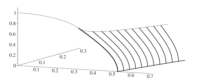
Figure 2: Phase diagram of QCD for $N_{f}=2$ light flavours, from [65].

Using the input of $T_{c}=160$ MeV and $\mu_{1}=1200$ MeV physical scales can be reintroduced, leading to a prediction for the location of a tricritical point.

Some remarks are in order. The same phase diagram has been obtained from several other models as reviewed in [68], as well as partly from Lattice simulations along the $T$-axis and close to $T_{c}$ following the transition (crossover) line (see [29, 32] for references). However, there is no flavour dependence in this MM prediction as the dependence of the sigma model on $N_{f}$ is too weak: the phase diagram looks the same also for any number $N_{f}>2$, given there is no other saddle point than $Q=\phi\,1\!|$. On the other hand for $N_{f}=3$ flavours we know from Lattice studies that for zero $\mu$ the transition at $T_{c}$ depends on the masses, e.g. for equal mass it becomes first order. We refer to [69] for a recent review. As a further restriction ${\langle\bar{q}q\rangle}$ is a fixed, $N_{f}$ independent input parameter in our MM. Because of the difficulties of performing Lattice simulations with a complex action, the presence or absence of a tri-critical point is still a subject of debate today (see [32] for a most recent critical review).

The MM can be refined by including different chemical potentials for the quarks, that is baryon $(\mu_{B})$ and isospin ($\mu_{I}$) chemical potential. This analysis has been carried out in [67] for $N_{f}=2$ including a very detailed analysis of the phase diagram. We only cite the most prominent feature, that is a doubling of the phase transition lines for fixed $\mu_{I}$ and mass $m$ as shown in fig. 3.

Figure 3: Phase diagram of QCD for $N_{f}=2$ light flavours in the $\mu_{B}$ plane for fixed $\mu_{I}$ and mass $m$, from [67]. All quantities are in units of the inverse variance $G$.

This can be easily understood as for $\mu_{1}\neq\mu_{2}$ the chiral restoration for the up and down quark condensates $\langle\bar{u}u\rangle$ and $\langle\bar{d}d\rangle$ is different. A similar effect can be expected if the masses are split, $m_{u}\neq m_{d}$, at equal chemical potential $\mu_{1}=\mu_{2}$. The same split of one first order transition into two was found analytical from MMs at $T=0$ [54], as can be derived from eq. (2.7) of the previous section. It leads to the fact that the $N_{f}$-flavour partition function can be written as a determinant of single flavour partition functions. In consequence the $N_{f}$-flavour partition function undergoes a transition whenever one of its building blocks, a single flavour partition function, has a phase transition (singular derivative).

4 Exact Limit: QCD Dirac Operator Spectrum

In this section we consider our MM as an exact limit of QCD, in the sense that it coincides with the $\epsilon$-regime of $\chi$PT as has been pointed out in subsection 2.2. This assumes that $\chi$PT as an effective theory itself can be consistently derived from QCD. In all the following we will consider temperature $T=0$ only.

4.1 Chiral symmetry and the Dirac spectrum

To start we recall the relation between the spectral density of the Dirac operator and spontaneous chiral symmetry breaking from field theory, both for zero and non-zero $\mu$. Throughout this subsection no reference to MM results is made, apart from figs. 4 and 5.

Let us begin by defining the spectral density of Dirac operator eigenvalues eq. (2.3) by

$$\rho_{\hbox to0.0pt{ $\,\raisebox{0.45206pt}{/}\hss$}D}(z)\ \equiv\ \left\langle\sum_{k}\delta^{2}(z_{k}-z)\right\rangle_{QCD}\ ,$$ (4.1)

where the average is taken over the gauge fields including the $N_{f}$ Dirac determinants. In our conventions the eigenvalues $z_{k}$ are real at $\mu=0$. In the same way higher order correlation functions can be defined, such as density-density correlations, etc. . In a finite volume on the Lattice there is only a finite number of discrete Dirac eigenvalues. When computing integrals at $\lim_{V\to\infty}$ with such an operator, such as sum-rules eq. (2.15), special care has to be taken for UV divergencies, and we refer to [70] for this issue at $\mu=0$. Putting QCD on the Lattice always provides a natural regularisation here. Because of chiral symmetry

$$\{(\hbox to0.0pt{ $\,\raisebox{0.6458pt}{/}\hss$}D+\mu\gamma_{0}),\gamma_{5}\}\ =\ 0\ ,$$ (4.2)

eigenvalues of $(\hbox to0.0pt{ $\,\raisebox{0.6458pt}{/}\hss$}D+\mu\gamma_{0})$ come in pairs $\pm iz_{k}$ as for each eigenfunction $\varphi_{k}$ of a non-zero eigenvalue there is also an eigenfunction $\gamma_{5}\varphi_{k}$ with eigenvalues $-iz_{k}$, except for $z_{k}=0$. The number of zero eigenvalues relates to the topological charge, $\nu=|n_{L}-n_{R}|$.

Because of this we can write for the resolvent

$$\Sigma(m)\equiv\left\langle\sum_{k}\frac{1}{iz_{k}+m}\right\rangle_{QCD}=\left\langle\sum_{k}{}^{\prime}\frac{2m}{z_{k}^{2}+m^{2}}\right\rangle_{QCD}\ +\ \langle\nu\rangle\frac{1}{m}\ .$$ (4.3)

where the second sum $\Sigma^{\prime}$ goes only over the non-zero eigenvalues with $-\pi/2<$Arg$(z_{k})\leq\pi/2$, the half plane $\mathbb{C}_{+}$. Here $m$ is an auxiliary mass. The partition function of course depends also on the $N_{f}$ masses $m_{f}$, see also the discussion after eq. (4.35). The chiral condensate is then defined as

$${\langle\bar{q}q\rangle}\equiv-\lim_{m\to 0}\lim_{V\to\infty}\Sigma(m)\ ,$$ (4.4)

where the order of limits is important. Using the electrostatic analogy $\Sigma(m)$ is the electric field for charges $iz_{k}$ on the imaginary axis for $\mu=0$, or on a stripe parallel to it for $\mu\neq 0$. The fact that chiral symmetry is broken trough the chiral condensate ${\langle\bar{q}q\rangle}$ corresponds to a jump of $\Sigma(m)$ along this axis, see fig. 4 below.

	$\mu=0$	$\mu\neq 0$
$\Sigma(m)$	$\lim_{n\to 0}\frac{1}{n}\partial_{m}\langle\det(\hbox to0.0pt{ $\,\raisebox{0.6458pt}{/}\hss$}D+m)^{n}\rangle_{QCD}$	$\lim_{n\to 0}\frac{1}{n}\partial_{m}\langle\det|\hbox to0.0pt{ $\,\raisebox{0.6458pt}{/}\hss$}D(\mu)+m|^{2n}\rangle_{QCD}$
$\lim_{V\to\infty}\Sigma(m)$	$\int_{0}^{\infty}dx\ \rho_{\hbox to0.0pt{ $\,\raisebox{0.45206pt}{/}\hss$}D}(x)\frac{2m}{x^{2}+m^{2}}$	$\int_{\mathbb{C}_{+}}d^{2}z\ \rho_{\hbox to0.0pt{ $\,\raisebox{0.45206pt}{/}\hss$}D}(z)\frac{2m}{z^{2}+m^{2}}$
$\rho_{\hbox to0.0pt{ $\,\raisebox{0.45206pt}{/}\hss$}D}(z=x+iy)$	$\lim_{\epsilon\to 0}\left.\frac{1}{2\pi i}[\Sigma(im+\epsilon)-\Sigma(im-\epsilon)]\right|_{m=x}$	$\left.\partial_{m^{*}}\Sigma(m)\right|_{m=z}$

Table 3: The resolvent and spectral density for zero and non-zero $\mu$. Here $m$ is an auxiliary mass, the $N_{f}$-dependence of $\rho_{/\!\!\!\!D}$ and $\Sigma(m)$ has been suppressed.

The relation between resolvent and spectral density however is different for $z_{k}$ real or complex, as summarised in table 3. For zero chemical potential we have

$$\lim_{V\to\infty}\Sigma(m)=\int_{0}^{\infty}dx\rho_{\hbox to0.0pt{ $\,\raisebox{0.45206pt}{/}\hss$}D}(x)\frac{2m}{x^{2}+m^{2}}\ ,$$ (4.5)

with $x\in\mathbb{R}_{+}$, assuming that $\langle\nu^{2}\rangle\sim V$ is suppressed. This leads to the Banks-Casher [71] relation in the chiral limit

$$|{\langle\bar{q}q\rangle}|=\frac{\pi}{V}\rho_{\hbox to0.0pt{ $\,\raisebox{0.45206pt}{/}\hss$}D}(0)\ ,$$ (4.6)

where we have used the representation $\lim_{m\to 0}\frac{2m}{x^{2}+m^{2}}=\pi\delta^{1}(x)$ of the 1-dimensional delta-function. On the right hand side of eq. (4.6) we have the macroscopic density of Dirac eigenvalues at zero momentum. Its slope has also been computed in [48], $\rho_{\hbox to0.0pt{ $\,\raisebox{0.45206pt}{/}\hss$}D}^{\prime}(x=0)=\frac{{\langle\bar{q}q\rangle}^{2}}{16\pi^{2}F_{\pi}^{4}}\frac{(N_{f}-2)(N_{f}+\beta_{D})}{N_{f}\beta_{D}}$, depending on the symmetry class through the Dyson index. Because of eq. (4.6) the smallest eigenvalues are spaced like $1/V$ (in contrast to free eigenvalues $\sim 1/V^{\frac{1}{4}}$) and we define a microscopic density, both for $\mu=0$ and $\mu\neq 0$,

$$\rho_{S}(\xi)\equiv\rho_{\hbox to0.0pt{ $\,\raisebox{0.45206pt}{/}\hss$}D}(\xi=z/{\langle\bar{q}q\rangle}V)/{\langle\bar{q}q\rangle}V\ .$$ (4.7)

This microscopic density can be obtained from eq. (4.5) by inverting the integral equation - if $\rho(x)$ is independent of the valence or source quark mass $m$- as the discontinuity of the resolvent:

$$\rho_{\hbox to0.0pt{ $\,\raisebox{0.45206pt}{/}\hss$}D}(x)=\lim_{\varepsilon\to 0}\frac{1}{2\pi i}[\Sigma(ix+\varepsilon)-\Sigma(ix+\varepsilon)]\ .$$ (4.8)

On the other hand for non-zero $\mu$ we have

$$\lim_{V\to\infty}\Sigma(m)=\int_{\mathbb{C}_{+}}d^{2}z\ \rho_{\hbox to0.0pt{ $\,\raisebox{0.45206pt}{/}\hss$}D}(z)\frac{2m}{z^{2}+m^{2}}\ .$$ (4.9)

Here the chiral limit $m\to 0$ does not produce the 2-dimensional delta-function $\pi\delta^{2}(z)=\partial_{z^{*}}\frac{1}{z}$. The density - resolvent relation in the complex plane instead reads:

$$\rho_{\hbox to0.0pt{ $\,\raisebox{0.45206pt}{/}\hss$}D}(z)=\frac{1}{\pi}\partial_{z^{*}}\Sigma(z)$$ (4.10)

that is outside the support the resolvent is holomorphic and inside it depends on the complex conjugate $z^{*}$. For more details we refer to [72]. When adding a delta-function $\delta^{1}(y)$ to eq. (4.8) we could also write it in the form of eq. (4.10).

So far we have only defined the microscopic density and the resolvent, and related the two. The question remains of how to compute them from field theory. We give two possibilities, replicas and supersymmetry, where again we have to distinguish $\mu=0$ and $\mu\neq 0$. Here extra fermionic and bosonic valance or source quarks are added to generate the resolvent.

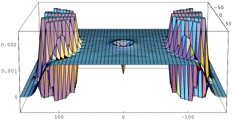
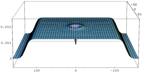
Figure 4: The microscopic spectral density $\rho_{S}^{(N_{f},v)}(\xi)$ at large volume, cut perpendicular to the real axis and rotated by $\pi/2$: the real part of the complex valued, unquenched density from MMs for $N_{f}=1$ flavour with mass $m{\langle\bar{q}q\rangle}V=80$ (upper plots) vs. the quenched density from $\epsilon\chi$PT (lower plots), both at rescaled $\mu F_{\pi}\sqrt{V}=8$. The resolvent $\Sigma(m{\langle\bar{q}q\rangle}V)$ obtained numerically is shown for comparison. All plots are from the second ref. of [74], with $\Sigma\equiv{\langle\bar{q}q\rangle}$.

In the supersymmetric approach at $\mu=0$ we can write

$$\Sigma(m)=\left.\partial_{m_{1}}\left\langle\frac{\det(\hbox to0.0pt{ $\,\raisebox{0.6458pt}{/}\hss$}D+m_{1})}{\det(\hbox to0.0pt{ $\,\raisebox{0.6458pt}{/}\hss$}D+m_{2})}\right\rangle_{QCD}\right|_{m_{1}=m_{2}}\ ,$$ (4.11)

using the fact that $\det(\hbox to0.0pt{ $\,\raisebox{0.6458pt}{/}\hss$}D+m)=\exp[\mbox{Tr}\log(\hbox to0.0pt{ $\,\raisebox{0.6458pt}{/}\hss$}D+m)]$. Here $m_{1}$ and $m_{2}$ are 1 extra fermionic and 1 bosonic quark, respectively. As long as $m_{2}$ has a small imaginary part, the generating functional containing the ratio of determinants in addition to the $N_{f}$ flavours is well defined. In the limit of $\epsilon\chi$PT we obtain an integral over the super Riemannian manifold $Gl(N_{f}+1|1)$ generalising eq. (2.8), and we refer to [19] for details.

For $\mu\neq 0$ the inverse determinant can no longer be regularised by an imaginary part, as the spectrum of $\hbox to0.0pt{ $\,\raisebox{0.6458pt}{/}\hss$}D(\mu)$ now extends into the complex plane. Here the so-called Hermitisation technique is used as follows. Defining

$${\cal Z}^{(N_{f}+2|2,\nu)}(m_{1},m_{2};\kappa)\equiv\left\langle\frac{\det[(\hbox to0.0pt{ $\,\raisebox{0.6458pt}{/}\hss$}D(\mu)+m_{1})(\hbox to0.0pt{ $\,\raisebox{0.6458pt}{/}\hss$}D(\mu)+m_{1})^{\dagger}+\kappa^{2}]}{\det[(\hbox to0.0pt{ $\,\raisebox{0.6458pt}{/}\hss$}D(\mu)+m_{2})(\hbox to0.0pt{ $\,\raisebox{0.6458pt}{/}\hss$}D(\mu)+m_{2})^{\dagger}+\kappa^{2}]}\right\rangle_{QCD},$$ (4.12)

we can obtain the regularised resolvent by differentiation and setting arguments equal as before, and then the density through eq. (4.10):

$$\rho_{\hbox to0.0pt{ $\,\raisebox{0.45206pt}{/}\hss$}D}(z)=\left.-\frac{1}{\pi}\lim_{\kappa\to 0}\partial_{m_{1}^{*}}\lim_{m_{2}\to m_{1}}\partial_{m_{2}}{\cal Z}^{(N_{f}+2|2,\nu)}(m_{1},m_{2};\kappa)\right|_{m_{1}=z}$$ (4.13)

For a detailed calculation in a non-chiral MM framework we refer to [75].

When using replicas the logarithm of the determinant is generated by inserting $n$ fermionic determinants of degenerate mass (replicas) into the partition function, leading to the resolvent as follows:

$$\Sigma(m)=\lim_{n\to 0}\frac{1}{n}\partial_{m}\left\langle\det(\hbox to0.0pt{ $\,\raisebox{0.6458pt}{/}\hss$}D+m)^{n}\right\rangle_{QCD}.$$ (4.14)

We will not comment here on the subtlety of analytically continuing $n\to 0$, as we will not use replicas in our computations. Eq. (4.14) is only valid for real eigenvalues at $\mu=0$. For $\mu\neq 0$ the appropriate replica limit includes complex conjugated quarks

$$\Sigma(m)=\lim_{n\to 0}\frac{1}{n}\partial_{m}\left\langle\det[(\hbox to0.0pt{ $\,\raisebox{0.6458pt}{/}\hss$}D(\mu)+m)^{n}(\hbox to0.0pt{ $\,\raisebox{0.6458pt}{/}\hss$}D(\mu)+m)^{{\dagger}\,n}]\right\rangle_{QCD}.$$ (4.15)

This was pointed out by Stephanov in [42] to explain the failure of the quenched approximation in LGT at $\mu\neq 0$. Using MM eq. (2.5) he showed that the critical potential is proportional to the pion mass, $\mu_{c}\sim m_{\pi}$, due to the presence of conjugated quarks in the correct replica limit eq. (4.15). This has to be compared with a third of the lightest Baryon mass, $\mu_{c}^{2}\sim m_{B}/3$, expected for unquenched QCD. Replicas for non-hermitian MMs and $\epsilon\chi$PT have been introduced in [73, 59] to compute correlation functions, using a relation to integrable hierarchies to make the replica limit exact.

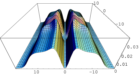
Figure 5: The same cut as in fig. 4 for the quenched density in the $\beta_{D}=4$ or adjoint QCD class from MMs at rescaled $\mu F_{\pi}\sqrt{V}=2.5$ and topology $\nu=0$. The corresponding resolvent is shown for positive arguments only.

We close this section by giving cuts through the microscopic densities in the large volume limit as obtained from MMs in the following sections. This is to illustrate the different symmetry classes and the effect of unquenching. Parallel to that the resulting resolvent is shown.

As was pointed out in [74] the strong oscillations in the complex valued unquenched spectral density are made responsible for chiral symmetry breaking, with a discontinuous resolvent. For comparison the quenched density and its continuous resolvent are shown as well in fig. 4. Here the chiral condensate is vanishing in the chiral limit and thus not responsible for symmetry breaking. It is the diquark condensate breaking chiral symmetry in this case.

We also give a cut through the quenched density for adjoint QCD. The resulting resolvent is again smooth as in quenched QCD above. This implies that the chiral condensate ${\langle\bar{q}q\rangle}$ is rotated to zero, with chiral symmetry being broken through a diquark condensate.

4.2 Complex Dirac eigenvalue correlation functions from MMs

In this section we will show how to derive complex eigenvalue correlation functions from MMs using orthogonal polynomials in the complex plane. The reason we choose this technique is that it is simple and carries over with little technical modifications to symplectic MMs or adjoint QCD in the next section. The alternative techniques are replicas using the Toda lattice, which has been successful only in the $\beta_{D}=2$ class, and supersymmetry. They will be mentioned only very briefly.

Our starting point is the two-MM version of the partition function eq. (2.5) based on eq. (2.4), that was first introduced in [50] (see also [63] for details)

$${\cal Z}^{(N_{f},\nu)}=\int d\Phi d\Psi_{N\times(N+\nu)}\prod_{f=1}^{N_{f}}\det\left(\begin{array}[]{cc}m_{f}&\Phi+\mu\Psi\\ -\Phi^{\dagger}+\mu\Psi^{\dagger}&m_{f}\\ \end{array}\right)e^{-N\mbox{Tr}(\Phi\Phi^{\dagger}+\Psi\Psi^{\dagger})}.$$ (4.16)

In order to obtain a complex eigenvalue model a Schur decomposition for the following complex matrices is performed, $C=\Phi+\mu\Psi=U(X+R)V$ and $D=-\Phi^{\dagger}+\mu\Psi=V^{\dagger}(Y+S)U^{\dagger}$. Here $X$ and $Y$ are diagonal matrices of complex eigenvalues $x_{k}$ and $y_{k}$. $R$ and $S$ are complex upper triangular matrices, $U$ and $V$ are unitary. The Jacobian is proportional to $\Delta_{N}(\{z^{2}\})=\prod_{j>k}^{N}(z_{j}^{2}-z_{k}^{2})$, the Vandermonde determinant. Because of the Gaussian measure the matrices $R$ and $S$ decouple and can be integrated out. A change of variables to the complex Dirac eigenvalues $z_{k}=x_{k}y_{k}$ of the matrix $CD$ is made next, and finally one of the 2 complex eigenvalue sets, $\{x_{k}\}$ is integrated out. This last step is transforming part of the Gaussian measure into a $K$-Bessel function:

$${\cal Z}^{(N_{f},\nu)}=\int_{\mathbb{C}}\prod_{j=1}^{N}d^{2}z_{j}\prod_{f=1}^{N_{f}}m_{f}^{\nu}(z_{j}^{2}+m_{f}^{2})\ |z_{j}|^{2\nu+2}K_{\nu}\left(\frac{N(1+\mu^{2})}{2\mu^{2}}|z_{j}|^{2}\right)e^{\frac{N(1-\mu^{2})}{4\mu^{2}}(z_{j}^{2}+z_{j}^{*\,2})}|\Delta_{N}(\{z^{2}\})|^{2}\ .$$ (4.17)

Here we have omitted all normalisation constants as they will drop out later in correlation functions. An approximation to this complex eigenvalue model was first introduced in [76] replacing $K_{\nu}(x)\to\sqrt{\pi/(2x)}\ e^{-x}$ by its asymptotic value. The two models coincide at $\nu=\pm\frac{1}{2}$.

The concept of orthogonal polynomials (both on $\mathbb{R}$ and $\mathbb{C}$) to compute eigenvalue correlation functions relies on the following properties. Given a weight function $w(z,z^{*})$ on $\mathbb{C}$ such that all moments are finite we can define a set of monic polynomials $P_{k}(z)=z^{k}+{\cal O}(z^{k-1})$:

$$\int_{\mathbb{C}}d^{2}z\ w(z,z^{*})P_{k}(z)P_{l}(z)^{*}=\delta_{kl}\ h_{k}$$ (4.18)

where $h_{k}$ are the squared norms. For real positive weights the coefficients of the polynomials can easily be seen to be real, $P_{l}(z)^{*}=P_{l}(z^{*})$. Using invariance properties of determinants we can write the following identity:

$$\Delta_{N}(\{z^{2}\})\Delta_{N}(\{z^{*\,2}\})\ =\ \det_{1\leq k,l\leq N}[P_{k-1}(z_{l})]\det_{1\leq k,l\leq N}[P_{k-1}(z_{l}^{*})]\ =\ \prod_{j=0}^{N-1}h_{j}^{-1}\ \det_{1\leq k,l\leq N}[K_{N}(z_{k},z_{l}^{*})]$$ (4.19)

where we have defined the kernel of orthogonal polynomials

$$K_{N}(z_{k},z_{l}^{*})\ =\ \sum_{j=0}^{N-1}h_{j}^{-1}P_{j}(z_{k})P_{j}(z_{l}^{*})\ .$$ (4.20)

It enjoys the following self contraction and normalisation property:

$$\int_{\mathbb{C}}d^{2}z\ w(z,z^{*})K_{N}(z_{k},z^{*})K_{N}(z,z_{j}^{*}) = K_{N}(z_{k},z_{j}^{*})$$

$$\int_{\mathbb{C}}d^{2}z_{k}\ w(z_{k},z_{k}^{*})K_{N}(z_{k},z_{l}^{*}) = \left\{\begin{array}[]{lll}1&\mbox{if}&k\neq l\\ N&\mbox{if}&k=l\end{array}\right.\ .$$ (4.23)

For such kernels the following Theorem by Dyson (Theorem 5.2.1 in [44]) holds

$$\int_{\mathbb{C}}d^{2}z_{n}\ w(z_{n},z_{n}^{*})\det_{1\leq i,j\leq n}[K_{N}(z_{i},z_{j}^{*})]\ =\ (N-n+1)\det_{1\leq i,j\leq n-1}[K_{N}(z_{i},z^{*}_{j})]\ .$$ (4.24)

Choosing the polynomials orthogonal with respect to the weight

$$w^{(N_{f},\nu)}(z,z^{*})\equiv\prod_{f=1}^{N_{f}}(z^{2}+m_{f}^{2})\ |z|^{2\nu+2}K_{\nu}\left(\frac{N(1+\mu^{2})}{2\mu^{2}}|z|^{2}\right)\exp\left(\frac{N(1-\mu^{2})}{4\mu^{2}}(z^{2}+z^{*\,2})\right),$$ (4.25)

in eq. (4.17) we can apply the Dyson Theorem to compute all complex eigenvalues $k$-point correlation functions defined as

$$R^{(N_{f},\nu)}(z_{1},\ldots,z_{k}) \equiv \frac{N!}{(N-k)!}\frac{1}{{\cal Z}^{(N_{f},\nu)}}\int_{\mathbb{C}}\prod_{j=k+1}^{N}d^{2}z_{j}\prod_{l=1}^{N}w^{(N_{f},\nu)}(z_{l},z_{l}^{*})|\Delta_{N}(\{z^{2}\})|^{2}$$ (4.26)

$$= \prod_{l=1}^{k}w^{(N_{f},\nu)}(z_{l},z_{l}^{*})\det_{1\leq i,j\leq k}[K_{N}(z_{i},z^{*}_{j})]\ .$$ (4.27)

It expresses the original $(N-k)$-fold integral as a determinant of size $k\times k$ only. Thus in the large-$N$ limit we only have to compute the asymptotic of the kernel $K_{N}(z_{i},z_{j}^{*})$. Note that for brevity we have suppressed the dependence on the complex conjugated arguments $z_{1}^{*},\ldots,z_{k}^{*}$ and on the masses in the functions $R^{(N_{f},\nu)}$.

Let us give an example. For the quenched weight, $w^{(0,\nu)}(z,z^{*})$ with $N_{f}=0$ in eq. (4.25), the orthogonal polynomials are given by Laguerre polynomials in the complex plane [50]

$$P_{k}(z)\ =\ (-)^{k}\frac{k!}{N^{k}}(1-\mu^{2})^{k}L^{\nu}_{k}\left(\frac{Nz^{2}}{1-\mu^{2}}\right)\ .$$ (4.28)

For a proof of their orthogonality we refer to appendix A in [51]. The corresponding kernel is given by

$$K_{N}(z_{k},z_{l}^{*})\ =\ w(z_{k},z_{k}^{*})^{\frac{1}{2}}w(z_{l},z_{l}^{*})^{\frac{1}{2}}\frac{N^{\nu+2}}{\pi\mu^{2}(1+\mu^{2})^{\nu}}\sum_{j=0}^{N-1}\frac{j!}{(j+\nu)!}L^{\nu}_{j}\left(\frac{Nz^{2}}{1-\mu^{2}}\right)L^{\nu}_{j}\left(\frac{Nz^{*\,2}}{1-\mu^{2}}\right).$$ (4.29)

The orthogonal polynomials for weights including $N_{f}>0$ flavours and their kernel can be expressed in terms of the quenched quantities eqs. (4.28) and (4.29) using the technique of bi-orthogonal polynomials [77, 50], or ordinary orthogonal polynomials [78] in the case of a positive definite weight (corresponding to $N_{f}>0$ phase quenched flavours). From this all correlation functions follow for $N_{f}\neq 0$, and for most explicit expressions we refer to [63], see also eq. (4.40) below. The partition functions with $N_{f}$ flavours themselves can also be expressed in terms of the quenched polynomials and kernel [78], resulting into eq. (2.12) in the large-$N$ limit.

As pointed out in subsection 2.2 the MM only becomes equal to the chiral Lagrangian in the following large-$N$ limit. We rescale complex eigenvalues, masses and chemical potential as in eq. (2.9)

$$\xi_{j}\ =\ 2Nz_{j}\ ,\ \ \eta_{f}\ =\ 2Nm_{f}\ ,\ \ \mbox{and}\ \ \alpha^{2}\ =\ 2N\mu^{2}\ ,$$ (4.30)

which is denoted by the microscopic limit at weak non-Hermiticity. The concept of weak non-Hermiticity introduced in [79] for non-chiral MMs implies that $\mu^{2}$ vanishes at a rate $1/N$. There exists a different limit called strong non-Hermiticity with a different scaling for the eigenvalues, keeping $\mu^{2}={\cal O}(1)$. This leads out of the domain of the chiral Lagrangian, and we refer to [54] for details.

The microscopic spectral density in the large-$N$ limit eq. (4.30) is defined as follows

$$\rho_{S}^{(N_{f},\nu)}(\xi)\ =\ \lim_{N\to\infty}\frac{1}{2N}R^{(N_{f},\nu)}\left(z=\frac{\xi}{2N}\right)\ .$$ (4.31)

All higher order correlations are rescaled accordingly. The quenched microscopic density obtained from eq. (4.29) thus reads

$$\rho_{S}^{(0,\nu)}(\xi)=\frac{1}{2\pi\alpha^{2}}|\xi|^{2}K_{\nu}\left(\frac{|\xi|^{2}}{4\alpha^{2}}\right)e^{\frac{\xi^{2}+\xi^{*\,2}}{8\alpha^{2}}}\int_{0}^{1}dt\ t\ e^{-2\alpha^{2}t^{2}}J_{\nu}(t\xi)J_{\nu}(t\xi^{*})\ .$$ (4.32)

In the Hermitian limit $\alpha\to 0$ it reduces to the density of real eigenvalues $\rho_{S}^{(0,\nu)}(\xi_{x})$ [1] times $\delta^{1}(\Im m(\xi))$

$$\rho_{S}^{(0,\nu)}(\xi_{x})\ \sim\ |\xi_{x}|\int_{0}^{1}dt\ t\ J_{\nu}(t\xi_{x})^{2}\ =\ \frac{\xi_{x}}{2}(J_{\nu}(\xi_{x})^{2}-J_{\nu-1}(\xi_{x})J_{\nu+1}(\xi_{x}))\ ,$$ (4.33)

where $\Re e(\xi)=\xi_{x}$ denotes the real part. Fig. 6 compares the two functions for different values of $\nu$ and $\alpha$.

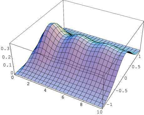
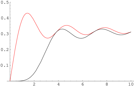
Figure 6: The quenched microscopic density eq. (4.32) at $\alpha=0.4$ for $\nu=0$ (top left) and $\nu=2$ (top right), and at $\alpha=3.28$ for $\nu=0$ (bottom right). For comparison we also show the density of real eigenvalues eq. (4.33) (bottom left) for $\nu=0$ (left curve) and $\nu=2$ (right curve), respectively. Note that in the complex plane the normalisation becomes a delta-function in the Hermitian limit $\alpha\to 0$.

For small $\alpha$ the density in the complex plane eq. (4.32) is very similar to the real one eq. (4.33), times a Gaussian decay in imaginary direction. Introducing exact zero eigenvalues by increasing $\nu$ pushes the density away from the origin through level repulsion. For increasing $\alpha$ the density quickly becomes a constant along a strip as from mean field, washing out the oscillations.

For the microscopic partition function with $N_{f}$ flavours we obtain eq. (2.14) which is $\mu$-independent for $B=1\!|$ as it should. We can now check that the same sum rule eq. (2.15) indeed follows from the quenched density eq. (4.32):

$$\frac{1}{4\nu}\ =\ \int_{\mathbb{C}}d^{2}\xi\ \frac{1}{\xi^{2}}\ \rho_{S}^{(0,\nu)}(\xi)\ \ \mbox{for}\ \ \nu\geq 1\ ,$$ (4.34)

which we have confirmed numerically up to $\nu=5$ for two different values of $\alpha<1$. Thus despite that for $\mu\neq 0$ the eigenvalues spread into the complex plane the sum rule remains unchanged. An analytic check, in particular of the unquenched, massive sum rules [60] using the complex valued densities for $N_{f}\geq 1$ given below would be highly desirable as well. For $\mu=0$ the Leutwyler-Smilga sum rule eq. (2.15) was shown analytically to follow from the real density eq. (4.33) [80].

Before turning to more flavours let us comment on other methods of deriving complex eigenvalue correlations and their relation to field theory. As was pointed out in subsect. 4.1 the spectral density can also be derived using replicas [59]

$$\rho_{S}^{(N_{f},\nu)}(\xi)\ =\ \lim_{n\to 0}\frac{1}{n\pi}\partial_{\xi^{*}}\partial_{\xi}\log[{\cal Z}^{(N_{f}+2n,\nu)}(\{\eta\},\{i\xi,i\xi^{*}\})]\ ,$$ (4.35)

where the first derivative generates the resolvent. Using replicas for complex eigenvalues (see table 3) we have introduced $n$ pairs of complex conjugate quarks of masses $i\xi$ and $i\xi^{*}$ respectively, having opposite $\mu$. Thus the corresponding partition functions eq. (2.12) now depend on $\mu$. It was shown in [59] that such partition functions obey the Toda Lattice equation

$$\frac{1}{n\pi}\xi^{*}\partial_{\xi^{*}}\xi\partial_{\xi}{\cal Z}^{(N_{f}+2n,\nu)}(\{\eta\},\{\xi,\xi^{*}\})\ =\ \frac{1}{2}(\xi\xi^{*})^{2}\frac{{\cal Z}^{(N_{f}+2n+2,\nu)}(\{\eta\},\{\xi,\xi^{*}\}){\cal Z}^{(N_{f}+2n-2,\nu)}(\{\eta\},\{\xi,\xi^{*}\})}{({\cal Z}^{(N_{f}+2n,\nu)}(\{\eta\})(\{\eta\}))^{2}}\ ,$$ (4.36)

leading to

$$\rho_{S}^{(N_{f},\nu)}(\xi)\ =\ \frac{1}{2}\xi\xi^{*}\frac{{\cal Z}^{(N_{f}+2,\nu)}(\{\eta\},\{i\xi,i\xi^{*}\}){\cal Z}^{(N_{f}-2,\nu)}(\{\eta\},\{i\xi,i\xi^{*}\})}{({\cal Z}^{(N_{f},\nu)}(\{\eta\}))^{2}}\ .$$ (4.37)

Here the minus 2 means that this partition function contains 2 conjugate bosons instead of fermions. In [64] the corresponding bosonic group integral given by eq. (2.16) was computed for $N_{f}=0$, thus deriving the quenched density from eq. (4.37) entirely from $\epsilon\chi$PT, without using knowledge from MMs. For $N_{f}\geq 1$ this result is still lacking, and using MMs we know that the corresponding group integral will factorise: ${\cal Z}^{(N_{f}-2,\nu)}(\{\eta\},\{\xi,\xi^{*}\})\sim{\cal Z}^{(N_{f},\nu)}(\{\eta\}){\cal Z}^{(-2,\nu)}(\{\xi,\xi^{*}\})$. The bosonic partition function has to be regularised and is proportional to the weight function eq. (4.25) to leading order. Using this as an input the equivalence of the Toda lattice and the orthogonal polynomials approach in MMs has been shown in [63], see eq. (4.40).

Another method to compute the spectral density is supersymmetry. Here the additional inverse determinants are introduced as Gaussian integrals over bosonic Grassmann variables, see the discussion after eq. (4.11), and then treated along the lines similar to subsect. 2.2. We refer to [81] where the equivalence of the supersymmetric and the Toda lattice approach was shown.

After comparing different techniques of solving MMs we would like to comment on the concept of universality. Sometimes the fact that instead of using a field theory such as $\epsilon\chi$PT to compute correlation functions one can use a simpler, chiral random MM, is called universality. As we have seen in sect. 2.2 these two are equivalent on the level of partition functions.

Here, we would like speak about MM universality, meaning that in the large-$N$ limit different MMs, Gaussian or non-Gaussian, containing 1 or 2 random matrices, lead to the very same eigenvalue correlation functions. What is know about universality for MM with complex eigenvalues? So far we know that the Gaussian one-MM eq. (2.5) and the Gaussian two-MM eq. (4.16) have the same partition functions for any number of $N_{f}$ fermions with chemical potentials $\pm\mu$, as well as the same quenched spectral density. Higher order and unquenched correlation functions have been obtained only in the second model.

At present little is known about the large-$N$ limit of non-Gaussian chiral MMs with complex eigenvalues. The determinantal [76, 50, 63] or Pfaffian structure [51, 82] of the correlations functions remain the same for non-Gaussian weights at finite-$N$, and from heuristic universality results [52] for the non-chiral complex ensemble at $\beta_{D}=2$ we expect that they are also universal.

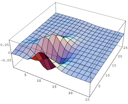
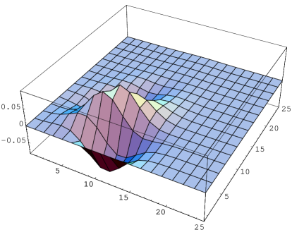
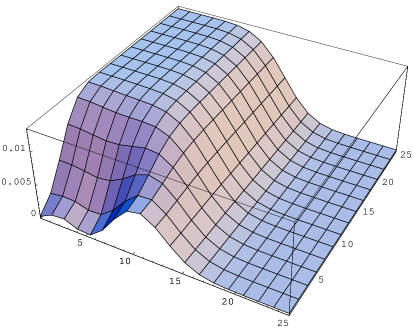
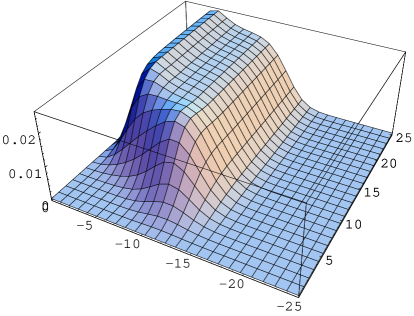
Figure 7: Comparison of densities for different theories in the first quadrant of $\mathbb{C}$ (rotated by $\pi/2$). Upper plots: the complex spectral density for unquenched QCD with $N_{f}=2$, $\Re e(\rho(z))$ (left) and $\Im m(\rho(z))$ (right), from [63]. Lower plots: phase quenched QCD (left) and adjoint QCD (right), both with $N_{f}=2$. All plots are at the same values $\alpha=2$, mass $\eta=5$.

We finish this subsection by giving the results for more flavours. With the definition

$${\cal I}_{\nu}(\xi_{1},\xi_{2})\ \equiv\ \int_{0}^{1}dt\ t\ e^{-2\alpha^{2}t^{2}}J_{\nu}(t\xi_{1})J_{\nu}(t\xi_{2})\ ,$$ (4.38)

the unquenched density for $N_{f}=1$ reads [63, 50]

$$\rho_{S}^{(N_{f}=1,\nu)}(\xi)=\rho_{S}^{(0,\nu)}(\xi)\left(1-\frac{J_{\nu}(\xi){\cal I}_{\nu}(i\eta,\xi^{*})}{J_{\nu}(i\eta){\cal I}_{\nu}(\xi,\xi^{*})}\right),$$ (4.39)

where we have factored out the quenched density. Note that the support of the quenched and unquenched density is the same. It can easily be seen that the density $\rho_{S}^{(N_{f}=1,\nu)}(\xi)$ is no longer real and positive. For general $N_{f}$ the structure remains the same : the factor multiplying the quenched density becomes a determinant of size $N_{f}+1$ [63, 50]:

$$\rho_{S}^{(N_{f},\nu)}(\xi)=\frac{1}{2\pi\alpha^{2}}|\xi|^{2}K_{\nu}\left(\frac{|\xi|^{2}}{4\alpha^{2}}\right)e^{\frac{\xi^{2}+\xi^{*\,2}}{8\alpha^{2}}}\prod_{f=1}^{N_{f}}(\eta_{f}^{2}+\xi^{2})\frac{{\cal Z}^{(N_{f}+2,\nu)}(\{\eta\},i\xi,i\xi^{*})}{{\cal Z}^{(N_{f},\nu)}(\{\eta\})}\ ,$$ (4.40)

where the additional pair “$+2$” has masses $i\xi$ and $i\xi^{*}$. The weight function originates from the bosonic partition function in the Toda lattice picture, and we refer to [63] for more details. It is not the explicit mass factor in front that makes the densities complex as it gets cancelled by the Vandermonde from eq. (2.12). We recall that the partition functions themselves become complex valued for complex mass arguments $\xi$.

For illustration we give the spectral density for $N_{f}=2$ in different theories. In the upper plots fig.7 real and imaginary part start displaying oscillation for moderate values of rescaled chemical potential. The spectral densities for phase quenched can also be computed using orthogonal polynomials, and we refer to [63] for details. For two phase quenched flavours with $|\det(\hbox to0.0pt{ $\,\raisebox{0.6458pt}{/}\hss$}D(\mu)+m)|^{2}$ the density with the very same parameter values is given in fig. 7 by the lower left plot. The oscillations have disappeared, with the real density simply vanishing at the locations of the mass. Note the difference in scale, the height of the supporting strip is hardly visible in the upper left plot. We also show the same unquenched density in the $\beta_{D}=4$ or adjoint class, from section 5. Apart from the additional repulsion from the axes it looks very similar to phase quenched QCD.

4.3 Comparison to quenched Lattice simulations

In this section we compare the predictions for complex eigenvalue correlation functions from the previous section to Lattice simulation. Because of the sign problem only quenched or phase quenched simulations can be compared with so far, and we will focus on the former. Phase quenched simulations with two flavours have been performed (see e.g. [83]) but the Dirac spectrum has not yet been compared to MMs.

The first comparison with the spectral density of quenched QCD on the lattice was performed in [84] for 3 different volumes $4^{4},\ 6^{4}$ and $10^{4}$ using staggered fermions at gauge coupling $\beta=6/g^{2}=5.0$ for chemical potentials varying from $\mu=10^{-3}-0.2$. The reason for choosing a rather strong coupling was to make the window in which MMs apply large enough for the small lattices studied. This assumed that the concept of a Thouless energy [22], the maximal eigenvalue up to which MMs and $\epsilon\chi$PT agree, can be generalised to $\mu\neq 0$. Evidence for this picture has been provided later from Lattice data in [57].

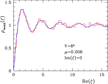
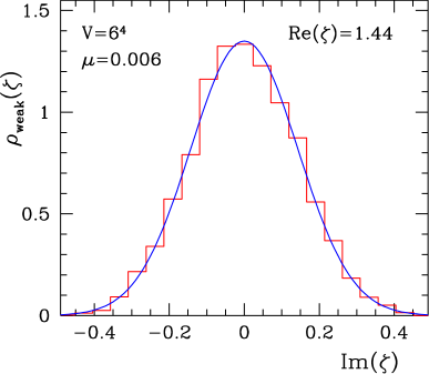
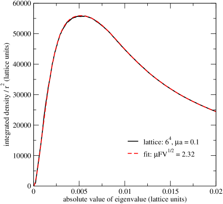
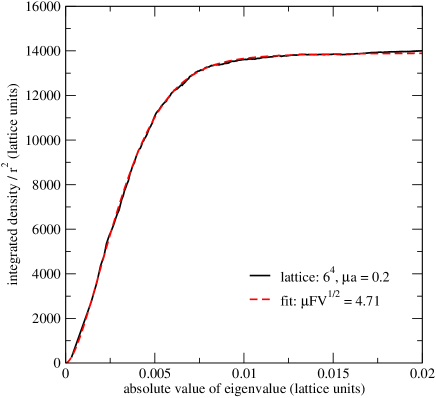
Figure 8: Comparison of the quenched density eq. (4.32) at $\alpha=0.2$ (full line) and Lattice data (histograms) for $V=6^{4}$ and $\mu=0.006$ (upper plots), from [84]. The left curve is cut along the real-axis, and the right curve is on the first maximum of the left curve, cut perpendicular to the real-axis.
Fitted integrated density (lower plots) eq. (4.41) vs. small Dirac eigenvalues from Lattice data [57] for $V=6^{4}$ and $\mu=0.1$ (left) and $\mu=0.2$ (right). The two curves are indistinguishable.

Instead of comparing to the 3-dimensional plots of fig. 6 we show cuts compared to data. For small $\alpha$ shown in fig. 8 we cut along the real axis and parallel to the imaginary axis on the first maximum. The agreement between the data and eq. (4.32) is excellent. In the plot the asymptotic form of the $K$-Bessel function in eq. (4.32) was used, as predicted from [76]. The exact expression eq. (4.32) was only found later in [59]. However, at the fitted value of $\alpha=0.200(2)$ the two curves are not distinguishable from the data (see fig. 1 in the second of ref. [59]).

For all other plots we use the exact density, eq. (4.32). The lower plots of fig. 8 from [57] show reanalysed and extended data from [84]. At larger values of $\alpha$ the density at the origin becomes asymptotically rotational invariant, see also fig. 9. Therefore the integrated density eq. (4.32)

$${\cal I}(r,\theta)=\int_{0}^{r}s\;ds\int_{0}^{\theta}d\phi~{}\rho_{S}(\xi=s\,{e}^{i\phi})~{}.$$ (4.41)

is compared to the data, finding again excellent agreement. Because of the rotational invariance only the ratio $\Sigma/F_{\pi}$ can be determined, and we refer to [57] for details.

Recently progress has been made concerning chiral fermions with chemical potential. In [85] it has been shown how to introduce $\mu\neq 0$ into the overlap operator [86] using a generalisation of the sign function in the complex plane. This opens up the possibility to compare to different topological sectors, and successful comparisons to the density eq. (4.32) have been made for $\nu=0$ and $\nu=1$ shown in fig. 9. Here the same cuts as in fig. 8 have been made (real and imaginary axis have been interchanged rotating by $\pi/2$), finding very good agreement. For the simulation and details of the complex overlap operator, in particular concerning the projection from the complex Ginsparg-Wilson circle to the complex plane we refer to [85].

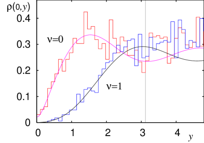
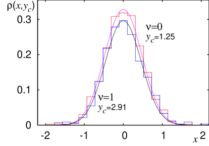
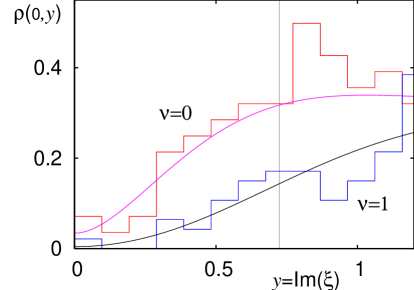
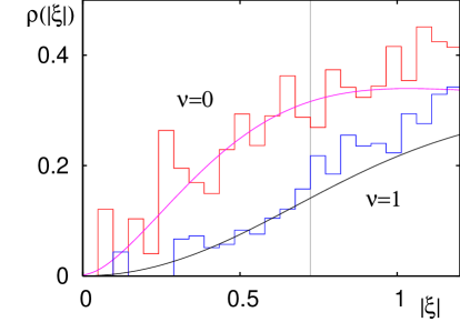
Figure 9: Cuts through the quenched density eq. (4.32) for topological sectors $\nu=0$ and 1, vs. Lattice data from [85] for $V=4^{4}$ and $\mu=0.1$ (upper plots) and $\mu=1.0$ (lower plots). ($x={\Re\mbox{e}}\xi$ and $y={\Im\mbox{m}}\xi$ are interchanged w.r.t. fig. 8). In the left plots the vertical bar indicates the fit range. For the largest value $\mu=1.0$ the density is almost rotational invariant, as indicated by the lower right plot fitted to the asymptotic density $\rho_{S}(|\xi|)=|\xi|^{2}/2\pi\alpha^{2}K_{\nu}(|\xi|^{2}/4\alpha^{2})I_{\nu}(|\xi|^{2}/4\alpha^{2})$. In this case only the ratio ${\langle\bar{q}q\rangle}/F_{\pi}$ can be fitted.

The results presented here are not the first comparisons between non-Hermitian MMs and Lattice data. In [87] quenched QCD lattice data were compared for a large range of $\mu$ to predictions of the non-chiral $\beta_{D}=2$ Ginibre ensemble for the spacing between eigenvalues in the complex plane. These predictions are only valid away from the origin where chiral symmetry is irrelevant, in the so-called bulk region. Here no relation to an effective theory as the chiral Lagrangian is known. A transition between the Wigner surmise for $\mu=0$, the Ginibre, and the Poisson distribution in the complex plane was found [87]. Unfortunately to date no prediction is known for the spacing or the distribution of individual eigenvalues in the origin region relevant for chiral symmetry breaking.

5 Adjoint QCD and Symplectic Matrix Model

In this section we summarise the known results for the $\beta_{D}=4$ symmetry class of matrices with quaternion real elements, being relevant for $SU(N_{C})$ gauge theories in the adjoint representation. In the first subsection 5.1 explicit results for the complex eigenvalue correlation functions are given. Since the methods are similar to the previous section we will be brief here, and only highlight the main differences: the fact that for $N_{f}\neq 0$ the densities remain real and positive as well as the different repulsion pattern of complex eigenvalues (see figs. 1 and 5). The positivity makes both quenched and unquenched lattice simulations possible, and a comparison to our MM predictions is done in the next subsection 5.2.

5.1 Complex eigenvalue correlations from a symplectic MM

Our starting point is the MM eq. (4.16) with the matrices having quaternion real elements instead. The very same procedure described in the previous section can be employed to achieve a complex eigenvalue model. We refer to [51] for details of the derivation where this ensemble was first defined. The MM partition function for $N_{f}$ flavours with equal chemical potential is reading in terms of complex eigenvalues

$${\cal Z}^{(N_{f},\nu)}(\{m_{f}\}) \sim \int\prod_{j=1}^{N}d^{2}z_{j}\prod_{f=1}^{N_{f}}m_{f}^{2\nu}|z_{j}^{2}+m_{f}^{2}|^{2}\ |z_{j}|^{4\nu+2}K_{2\nu}\!\left(\frac{N(1+\mu^{2})}{2\mu^{2}}|z_{j}|^{2}\right)e^{\frac{N(1-\mu^{2})}{4\mu^{2}}(z_{j}^{2}+z_{j}^{*\,2})}$$ (5.1)

$$\times\prod_{k>l}^{N}|z_{k}^{2}-z_{l}^{2}|^{2}\ |z_{k}^{2}-z_{l}^{\ast\,2}|^{2}\prod_{h=1}^{N}|z_{h}^{2}-z_{h}^{\ast\,2}|^{2}\ .$$

There are two main differences to eq. (4.17) for $\beta_{D}=2$. First, the mass term is automatically positive definite here because the eigenvalues of quaternion real matrices always come in complex conjugated pairs [44]. It thus resembles QCD with pairs of $N_{f}$ conjugated flavours also called phase quenched (see fig. 7). The same pairing of eigenvalues is also true for the zero modes, leading to a shift $\nu\to 2\nu$ compared to QCD. Second, the Jacobian is different from the squared absolute value of the Vandermonde determinant for $\beta_{D}=2$. The last factor in eq. (5.1) leads to vanishing correlations along the $x$- and $y$-axis here, as $|z_{h}^{2}-z_{h}^{\ast\,2}|^{2}=16x_{h}^{2}y_{h}^{2}$ vanishes there. We will find this feature explicitly in our results for the correlation functions, see fig. 10. In the limit $\mu\to 0$ for both $\beta_{D}=2,4$ the Jacobians reduce to $\Delta_{N}(x^{2})^{\beta_{D}}$, counting the number of independent degrees of freedom per matrix element.

The complex eigenvalue correlation functions are defined in complete analogy to eq. (4.26) with the corresponding weight and Jacobian. The result can be written as a Pfaffian [51, 82]

$$R^{(N_{f},\nu)}(z_{1},\ldots,z_{k})\ =\ \prod_{j=1}^{k}(z_{j}^{\ast\,2}-z_{j}^{2})w(z_{j},z_{j}^{\ast})\ \mbox{Pf}_{i,j=1,\ldots,k}\left[\begin{array}[]{ll}\kappa_{N}(z_{i},z_{j})&\kappa_{N}(z_{i},z_{j}^{\ast})\\ \kappa_{N}(z_{i}^{\ast},z_{j})&\kappa_{N}(z_{i}^{\ast},z_{j}^{\ast})\end{array}\right]\ .$$ (5.2)

For antisymmetric matrices $A$ of even dimension the Pfaffian is the square root of the determinant, Pf$(A)=\sqrt{\det(A)}$. A similar form uses a quaternion determinant, see [82]. Here we have introduced the pre-kernel $\kappa_{N}(z_{1},z_{2}^{\ast})$,

$$\kappa_{N}(z_{1},z_{2}^{\ast})\ \equiv\ \sum_{k=0}^{N-1}\frac{1}{r_{k}}\left(q_{2k+1}(z_{1})q_{2k}(z_{2}^{\ast})-q_{2k+1}(z_{2}^{\ast})q_{2k}(z_{1})\right)\ ,$$ (5.3)

containing skew orthogonal polynomials $q_{k}(z)$. These are defined by the following skew-orthogonality relation

$$\int_{\mathbb{C}}d^{2}z\ w(z,z^{\ast})(z^{\ast\,2}-z^{2})\left[q_{2k+1}(z)q_{2l}(z^{\ast})-q_{2k+1}(z^{\ast})q_{2l}(z)\right]\ =\ r_{k}\ \delta_{kl}\ ,$$ (5.4)

where the remaining integrals with even/even and odd/odd indices vanish. For the quenched weight with $N_{f}=0$ above these polynomials are again given in terms of Laguerre polynomials in the complex plane [51],

$$q_{2k+1}(z)\ \sim\ L_{2k+1}^{2\nu}\left(\frac{Nz^{2}}{1-\mu^{2}}\right)\ ,\ \ \ \ q_{2k}(z)\ \sim\ \sum_{j=0}^{k}c_{j}(\mu)L_{2j}^{2\nu}\left(\frac{Nz^{2}}{1-\mu^{2}}\right),$$ (5.5)

with some known $\mu$-dependent coefficients $c_{j}(\mu)$ [51]. The unquenched correlation functions can again be expressed in terms of the quenched pre-kernel [51, 82], where for an odd number of $N_{f}$ flavours also the quenched skew orthogonal polynomials of even order $q_{2k}(z)$ explicitly appear [82].

The large-$N$ limit is defined by the same rescaling of the chemical potential, eq. (4.30), of the complex eigenvalues and masses, $\sqrt{2}\,z=\xi$ and $\sqrt{2}\,m=\eta$, and correspondingly of the microscopic density eq. (4.31). The simplest examples for the resulting correlation functions in the large-$N$ limit is the quenched microscopic spectral density

$$\rho_{S}^{(0,\nu)}(\xi)\ =\ \frac{1}{32\alpha^{4}}(\xi^{\ast\,2}-\xi^{2})\ |\xi|^{2}\ K_{2\nu}\left(\frac{|\xi|^{2}}{2\alpha^{2}}\right)\mbox{e}^{+\frac{1}{4\alpha^{2}}(\xi^{2}+\xi^{*\,2})}{\cal I}_{\nu}(\xi,\xi^{*})\ ,$$ (5.6)

where the limiting pre-kernel eq. (5.3) leads to a double integral here due to the extra sum in eq. (5.5) (compared to eq. (4.32) for $\beta_{D}=2$)

$${\cal I}_{\nu}(\xi,\xi^{*})\equiv\int_{0}^{1}ds\int_{0}^{1}\frac{dt}{\sqrt{t}}\ \mbox{e}^{-2s(1+t)\alpha^{2}}\left(J_{2\nu}(2\sqrt{st}\ \xi)J_{2\nu}(2\sqrt{s}\ \xi^{\ast})\ -\ J_{2\nu}(2\sqrt{s}\ \xi)J_{2\nu}(2\sqrt{st}\ \xi^{\ast})\right)\ .$$ (5.7)

Its antisymmetry together with the pre-factor $(\xi^{\ast\,2}-\xi^{2})$ leads to a real positive density eq. (5.6).

Our second example is the unquenched microscopic spectral density for $N_{f}=2$ flavours of degenerate masses:

$$\rho_{S}^{(N_{f}=2,\nu)}(\xi)\ =\ \rho_{S}^{(0,\nu)}(\xi)\left(1-\frac{{\cal I}_{\nu}(\xi^{*},i\eta){\cal I}_{\nu}^{\prime}(\xi,i\eta)-{\cal I}_{\nu}(\xi,i\eta){\cal I}_{\nu}^{\prime}(\xi^{*},i\eta)}{{\cal I}_{\nu}(\xi,\xi^{*}){\cal I}_{\nu}^{\prime}(i\eta,i\eta)}\right)\ ,$$ (5.8)

where

$${\cal I}_{\nu}^{\prime}(\xi,\xi^{*})\equiv\int_{0}^{1}\!ds\int_{0}^{1}dt\sqrt{\frac{s}{t}}\ \mbox{e}^{-2s(1+t)\alpha^{2}}\left(\sqrt{t}J_{2\nu+1}(2\sqrt{st}\ \xi)J_{2\nu}(2\sqrt{s}\ \xi^{*})-J_{2\nu}(2\sqrt{st}\ \xi^{*})J_{2\nu+1}(2\sqrt{s}\ \xi)\right)$$ (5.9)

is the derivative of the kernel eq. (5.7). It appears because of the degenerate masses in our example. Eq. (5.8) now contains 3 terms being a Pfaffian, and it is again explicitly real.

The quenched and unquenched densities eqs. (5.6) and (5.8) are compared in fig. 10 for different values of rescaled chemical potential $\alpha$ and mass $\eta$.

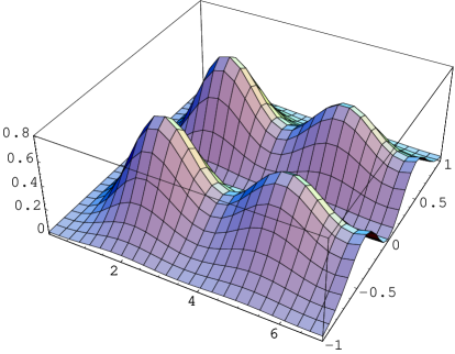
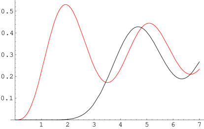
Figure 10: The quenched density eq. (5.6) (top left) vs. the unquenched density eq. (5.8) for $N_{f}=2$ flavours of equal rescaled mass $\eta=4.26$ (top right), both at $\nu=0$ for $\alpha=0.4$, and the unquenched density eq. (5.8) for $N_{f}=2$ at $\alpha=3.28$ and rescaled mass $\eta=19$ (bottom right). For comparison we also give the quenched density of real eigenvalues (bottom left) for $\nu=0$ (left curve) and $\nu=2$ (right curve), respectively.

The vanishing correlations along $x$- and $y$-axis due to the Jacobian is clearly observed. The introduction of masses has a mild effect, pushing the density further away from the origin when lowering the mass, without drastic change of its shape. At zero mass the resulting density becomes indistinguishable from the quenched density at $\nu=2$. However, this flavour-topology duality holds only approximately for $\mu\neq 0$ due to the explicit $\nu$-dependence of the $K$-Bessel weight.

For large values of $\alpha$ the density becomes almost constant along a strip, apart from the repulsion from the axis. In fig. 10 bottom right the mass at $\eta=19$ deforms this strip, as the location of the mass is a zero of the partition function, and of the density as well. The described effect of the masses on the density will be used in the next subsection to test the effect of unquenching in Lattice result.

Finally let us give the microscopic density for an arbritrary number of flavours:

$$\rho_{S}^{(N_{f},\nu)}(\xi)=\frac{1}{2\pi\alpha^{2}}(\xi^{*\,2}-\xi^{2})|\xi|^{2}K_{2\nu}\left(\frac{|\xi|^{2}}{4\alpha^{2}}\right)e^{\frac{z^{2}+z^{*\,2}}{8\alpha^{2}}}\prod_{f=1}^{N_{f}}|\eta_{f}^{2}+\xi^{2}|^{2}\frac{{\cal Z}^{(N_{f}+2,\nu)}(\{\eta\},i\xi,i\xi^{*})}{{\cal Z}^{(N_{f},\nu)}(\{\eta\})}\ ,$$ (5.10)

where the additional two flavours have masses $i\xi$ and $i\xi^{*}$. The structure is exactly the same as for the unquenched densities for QCD, eq. (4.40). The difference here is that due to the quaternion structure the extra complex mass pair $\xi$ and $\xi^{*}$ does not spoil the reality and positivity of the corresponding partition functions. For more details and higher order correlation functions we refer to [51, 82].

Let us close this subsection with a few remarks. For $\beta_{D}=4$ the complex eigenvalue correlation functions are simpler than the corresponding ones for $\mu=0$. This seemingly paradoxical statement originates in the simpler skew product and pre-kernel compared to the MM of real eigenvalues, explaining features of the latter [82].

In the previous section on the $\beta_{D}=2$ class several alternative and equivalent derivations of the same results have been stated. In our $\beta_{D}=4$ class to date no such alternative derivation is known so far using replicas, even for $\mu=0$. Also the supersymmetric method has only been applied to non-chiral MMs with $\beta_{D}=4$ (and $\beta_{D}=1$) [43], where the microscopic density was derived. For a complete solution from skew-orthogonal polynomials of this non-chiral MM we refer to [89]. As in the $\beta_{D}=2$ case a supersymmetric treatment would be simpler to do first in the one-MM eq. (2.5).

Consequently little is known about the universality of the microscopic correlation functions and their relation to field theory in this symmetry class (the same statement is true for $\mu=0$, except for all masses degenerate).

The only exception is for one pair of complex conjugate flavours $N_{f}=2$, where the same result for the partition function

$${\cal Z}^{(N_{f}=2,\nu)}_{\epsilon\chi PT}(\eta)\ \sim\ \int_{0}^{1}dt\ e^{-2t^{2}\alpha^{2}}I_{2\nu}(2t\eta)$$ (5.11)

can also be derived from the corresponding group integral in the $\epsilon\chi$PT [88]. For more general MM partition functions with $N_{f}>2$ we refer to [51, 82].

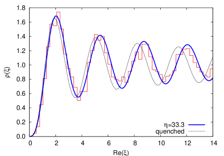
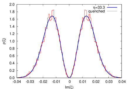
Figure 11: Lattice data (histograms) at mass $ma=0.07$ in lattice unit $a$, volume $V=6^{4}$ and $\mu=10^{-3}$ from [91], vs. MM prediction eq. (5.8) at $\alpha=0.0127$ (full curve). The cuts are made parallel to the $x$-axis along the maxima (left), and perpendicular to it on the first pair of maxima. For comparison the quenched curve eq. (5.6) is included as well, which is clearly shifted away from the data (left plot).

5.2 Comparison to unquenched Lattice data using staggered fermions for $SU(2)$

In this subsection we compare the complex eigenvalue correlation functions from the previous subsection to lattice simulations [90, 91]. Because for eigenvalues in the complex plane much statistics was needed staggered fermions were chosen in these simulations, using the code of [92]. In order to remain in the $\beta_{D}=4$ symmetry class while using staggered fermions this comparison is made between our symplectic MM results and an $SU(2)$ gauge theory in the fundamental representation realised as a staggered operator (see table 1). We recall that in the continuum $SU(2)$ in the fundamental representation belongs to the class $\beta_{D}=1$.

The lattice simulations [91] were done using two different volumes, $V=6^{4}$ and $8^{4}$ at fixed gauge coupling $\beta=1.3$ for chemical potentials ranging from $\mu=10^{-6}-0.2$. Starting at large masses where the smallest eigenvalues effectively quench [90] the masses were varied down to values where an effect of unquenching was observed. For more details of the simulations we refer to [91].

For a quantitative comparison we show cuts trough the 3 dimensional density plots of fig. 10: the curves are cut along the maxima parallel to the $x$-axis and on the (first) maximum perpendicular to that parallel to the $y$-axis.

For small $\alpha<1$ the effect of unquenching is only seen in the cut in $x$-direction through a shift of the curve, see fig. 11 left. The shift compared to the quenched curve from eq. (5.6) is clearly visible. Note that it is very difficult to perform simulations at sufficiently small mass. In the perpendicular direction which is used to fit $\alpha$ no difference to the quenched curve is seen (when appropriately normalised) as we expect. The data follow very nicely the MM prediction. A similar comparison was made for large quark masses in [90], nicely matching with the quenched result.

Turning to large values of $\alpha$ the situation is reversed. At the smallest mass values available the cut in $x$-direction is not distinguishable from quenched. However, the perpendicular cut in $y$-direction shows the deformation of the density through the mass, as is clearly seen in fig. 12. Since in this case the cut in $y$-direction is also used to fit $\alpha$, two different fits are compared: the $\alpha$ determined from the unquenched curve is compared to the quenched curve at the same value of $\alpha$, see the right curve in fig. 12. Second, a different value of $\alpha$ is obtained by directly fitting the quenched curve, leading however to a bigger mismatch in fig. 12 left, underscoring the data. Clearly the unquenched curve describes the data best.

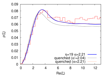
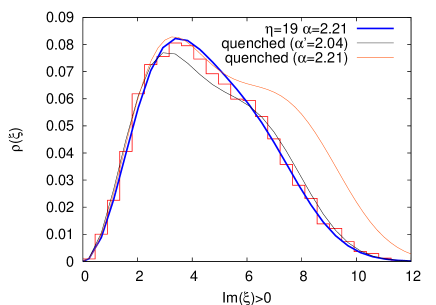
Figure 12: The same cuts as in fig. 11 but for larger $\alpha$: Lattice data (histograms) at mass $ma=0.06$, volume $V=6^{4}$ and $\mu=0.2$, from [91], versus MM prediction eq. (5.8) (full curve). For a better resolution we only display half of the cut in $y$-direction compared to fig. 11 (right). Here two different quenched densities from eq. (5.6) are inserted: the with the same $\alpha$ as unquenched, and a fit to the right cut. Both deviate from the data.

The same procedure has been repeated for different values of the mass and chemical potential in [91]. Comparing the two volumes and keeping the product $V\mu^{2}$ fixed confirms the scaling predicted by $\epsilon\chi$PT and MMs from the data in the $\beta_{D}=4$ symmetry class.

In previous Lattice simulations using staggered fermions for both classes $\beta_{D}=4$ and 1 [93] no comparison to MMs was available, and still is not for the latter class.

In summary we have seen that our symplectic MM is able to describe unquenched Lattice data in the case where the density remains real and positive.

6 Matrix Model of QCD with Imaginary Isospin Chemical Potential

In this section we discuss a MM for imaginary isospin chemical potential. The main difference to the previous MM is that is has real Dirac operator eigenvalues. This model was first introduced in [55] in terms of the corresponding $\epsilon\chi$PT. The motivation was to have a model that allows to determine the pion decay constant $F_{\pi}$ on the Lattice while keeping the Dirac eigenvalues real, in order to allow for unquenched simulations. The quenched results in [55] were then extended to the unquenched two-point function with $N_{f}=2$ and confirmed on the Lattice [56]. We note that $F_{\pi}$ can also be determined on the lattice for real $\mu$ using quenched QCD with complex Dirac eigenvalues [57, 84].

Here we follow the presentation of [62] (see also [58]) where the corresponding MM was introduced and solved for all unquenched correlations functions. The cases known from field theory [55, 56] were confirmed.

6.1 Real eigenvalue correlations

We start by writing down the Dirac operators for imaginary isospin chemical potential $\pm i\mu$:

$$\hbox to0.0pt{ $\,\raisebox{0.6458pt}{/}\hss$}D_{\pm}(\mu)=\left(\begin{array}[]{cc}0&\Phi\pm\mu\Psi\\ -(\Phi^{\dagger}\pm\mu\Psi^{\dagger})&0\end{array}\right)~{}.$$ (6.3)

For both signs it is anti-hermitian thus having real eigenvalues. The symmetry classification in table 1 is not affected by this rotation and thus we can immediately write down the MM for $m$ copies with $+i\mu$ and $n$ copies with $-i\mu$

$${\cal Z}^{(N_{f}=m+n,\nu)}\sim\int\!d\Phi d\Psi\prod_{f+=1}^{m}\!\det[\hbox to0.0pt{ $\,\raisebox{0.6458pt}{/}\hss$}D_{+}+m_{f+}]\!\prod_{f-=1}^{n}\!\det[\hbox to0.0pt{ $\,\raisebox{0.6458pt}{/}\hss$}D_{-}+m_{f-}]\ e^{-N{\rm Tr}\left(\Phi^{\dagger}\Phi+\Psi^{\dagger}\Psi\right)}\ .$$ (6.4)

However, for $\mu\neq 0$ the operators $\hbox to0.0pt{ $\,\raisebox{0.6458pt}{/}\hss$}D_{+}(\mu)$ and $\hbox to0.0pt{ $\,\raisebox{0.6458pt}{/}\hss$}D_{-}(\mu)$ now have different real eigenvalues (or more precisely real positive singular values): $\{x_{k}\}$ and $\{y_{k}\}\in\mathbb{R}_{+}$ respectively. After the change of variables

$$\Phi_{\pm}\ \equiv\ \Phi\pm\mu\Psi$$ (6.5)

the Gaussian weight becomes replaced by

$$V(\Phi_{+},\Phi_{-})=c_{+}(\Phi_{+}^{\dagger}\Phi_{+}+\Phi_{-}^{\dagger}\Phi_{-})-c_{-}\left(\Phi_{+}^{\dagger}\Phi_{-}+\Phi_{-}^{\dagger}\Phi_{+}\right)$$ (6.6)

where $c_{\pm}=(1\pm\mu^{2})/(4\mu^{2})$. A transformation to eigenvalues of this two-MM can thus only be performed for the $\beta_{D}=2$ symmetry class including QCD, to which we restrict ourselves in all the following. Only here the following matrix integral is available [94]

$$\int dUdV\exp\left[c_{-}N{\rm Tr}(VXUY)~{}~{}{\rm+~{}h.c.}~{}\right]~{}=~{}\frac{\det[I_{\nu}(2c_{-}Nx_{i}y_{j})]}{\prod(x_{i}y_{i})^{\nu}\Delta_{N}(\{x^{2}\})\Delta_{N}(\{y^{2}\})}~{}.$$ (6.7)

If we parametrise $\Phi_{+}=U_{+}XV_{+}$ and $\Phi_{-}=U_{-}YV_{-}$ and use the invariance of the Haar measure we obtain the following eigenvalue model:

$${\cal Z}^{(N_{f},\nu)}(\{m_{1}\},\{m_{2}\}) \sim \int_{0}^{\infty}\prod_{i=1}^{N}\left(dx_{i}dy_{i}(x_{i}y_{i})^{\nu+1}\prod_{f+=1}^{m}(x_{i}^{2}+m_{f+}^{2})\prod_{f-=1}^{n}(y_{i}^{2}+m_{f-}^{2})\right)$$ (6.9)

$$\times\Delta_{N}(\{x^{2}\})\Delta_{N}(\{y^{2}\})\det_{k,l}\left[I_{\nu}(2c_{-}Nx_{k}y_{l})\right]e^{-N\sum_{i}^{N}c_{+}(x_{i}^{2}+y_{i}^{2})}.$$

While for the partition function the determinant can be replaced by its diagonal part due to the antisymmetry of the Vandermonde determinants, this is not the case for the eigenvalue correlations. We note that also in this model the initial Gaussian weight has become non-Gaussian containing an $I$-Bessel function, due to the group integral performed.

The MM eq. (6.9) can be completely solved by introducing bi-orthogonal polynomials

$$\int_{0}^{\infty}dxdy\ w^{(N_{f})}(x,y)\ P_{n}^{(N_{f})}(x^{2})\ Q_{k}^{(N_{f})}(y^{2})=h_{n}^{(N_{f})}\delta_{nk}~{},$$ (6.10)

with respect to the weight function

$$w^{(N_{f})}(x,y)\ \equiv\ (xy)^{\nu+1}\prod_{f+=1}^{m}(x^{2}+m_{f+}^{2})\prod_{f-=1}^{n}(y^{2}+{m}_{f-}^{2})\ I_{\nu}\left(2c_{-}Nxy\right)e^{-Nc_{+}(x^{2}+y^{2})}\ .$$ (6.11)

The monic polynomials are in general different. Together with their integral transform

$$\chi_{k}^{(N_{f})}(y) \equiv \int_{0}^{\infty}dx\ w^{(N_{f})}(x,y)P_{k}^{(N_{f})}(x^{2})\ ,$$

$$\hat{\chi}_{k}^{(N_{f})}(x) \equiv \int_{0}^{\infty}dx\ w^{(N_{f})}(x,y)Q_{k}^{(N_{f})}(y^{2})\ .$$ (6.12)

four different kernels can be constructed

$$K_{N}^{(N_{f})}(y,x) = \sum_{k=0}^{N-1}\frac{Q_{k}^{(N_{f})}(y^{2})P_{k}^{(N_{f})}(x^{2})}{h_{k}}\ ,\ \ H_{N}^{(N_{f})}(x_{1},x_{2})\ =\ \sum_{k=0}^{N-1}\frac{\hat{\chi}_{k}^{(N_{f})}(x_{1})P_{k}^{(N_{f})}(x_{2}^{2})}{h_{k}}\ ,$$

$$M_{N}^{(N_{f})}(x,y) = \sum_{k=0}^{N-1}\frac{\hat{\chi}_{k}^{(N_{f})}(x)\chi_{k}^{(N_{f})}(y)}{h_{k}}\ ,\ \ \ \ \ \ \hat{H}_{N}^{(N_{f})}(y_{1},y_{2})\ =\ \sum_{k=0}^{N-1}\frac{Q_{k}^{(N_{f})}(y_{1}^{2})\chi_{k}^{(N_{f})}(y_{2})}{h_{k}}.$$ (6.13)

These are needed to express all correlation functions of mixed $x_{k}$ and $y_{l}$ eigenvalues defined as

$$R_{(n,k)}^{(N_{f},\nu)}(\{x\}_{n};\{y\}_{k}) \equiv \frac{N!^{2}}{(N-n)!(N-k)!}\frac{1}{{\cal Z}_{\nu}^{(N_{f})}(\{m_{1}\},\{m_{2}\})}$$ (6.14)

$$\times \int_{0}^{\infty}\prod_{i=n+1}^{N}dx_{i}\prod_{j=k+1}^{N}dy_{j}\det_{p,q}\left[w^{(N_{f})}(x_{p},y_{q})\right]\Delta_{N}(\{x^{2}\})\Delta_{N}(\{y^{2}\})$$

$$= \!\!\!\!\!\det_{1\leq i_{1},i_{2}\leq n;\ 1\leq j_{1},j_{2}\leq k}\!\left[\!\!\begin{array}[]{cc}H_{N}^{(N_{f})}(x_{i_{1}},x_{i_{2}})&M_{N}^{(N_{f})}(x_{i_{1}},y_{j_{2}})-w^{(N_{f})}(x_{i_{1}},y_{j_{2}})\\ K_{N}^{(N_{f})}(y_{j_{1}},x_{i_{2}})&\hat{H}_{N}^{(N_{f})}(y_{j_{1}},y_{j_{2}})\\ \end{array}\!\!\!\right]$$ (6.17)

In the definition in the first line we have written the integrand of eq. (6.9) in a more compact form. The solution in terms of a determinant of 4 blocks follows from [95], adopted to our chiral two-MM [62]. Note that in contrast to eqs. (4.27) and (5.2) the kernels built from the integral transforms of the polynomials contain part of the weight inside the determinant.

For $N_{f}\neq 0$ all polynomials, their transforms and the corresponding kernels can be expressed through the quenched quantities as detailed in [62]. Below we give the quenched quantities as an explicit simple example.

For the quenched weight $N_{f}=0$ in eq. (6.11) the bi-orthogonal polynomials are equal and both given by Laguerre polynomials of real variables:

$$P_{n}(x^{2})\ ,\ Q_{n}(x^{2}) \sim L_{n}^{\nu}\left(\frac{N}{1+\mu^{2}}x^{2}\right).$$ (6.18)

In addition the integral transforms also become proportional to Laguerre polynomials, times the Laguerre weight:

$$\chi_{k}(y)\ ,\ \hat{\chi}_{k}(y) \sim y^{2\nu+1}e^{-\frac{N}{1+\mu^{2}}y^{2}}L_{k}^{\nu}\left(\frac{N}{1+\mu^{2}}y^{2}\right).$$ (6.19)

The reason is that for this special case the bi-orthogonal polynomials and their weight can be constructed starting from two ordinary orthogonal Laguerre polynomials of a factorised weight, where for details we refer to appendix B of ref. [62].

We finish this subsection by giving two examples in the microscopic large-$N$ limit given by eq. (4.30). First, the partition function eq. (6.9) in this limit becomes identical to eq. (2.12), with the replacement $\mu^{2}\to-\mu^{2}$ in eq. (2.13) [62]. It agrees with the partition functions computed from $\epsilon\chi$PT field theory, simply because the effective chiral Lagrangian eq. (2.8) is obtained by this rotation to $B=i\mu$ diag$(1\!|_{m},-1\!|_{n})$. The group integral is convergent for both signs of $\mu^{2}$ and the rotation is trivial.

On the level of correlation functions however, this rotation is highly nontrivial. Leading to complex eigenvalues on the one side and two sets of real eigenvalues on the other side their determinantal structure is very different, comparing eqs. (4.27) and (6.17) above.

The simplest nontrivial correlation function is the quenched probability to find one eigenvalues $\xi$ of $\hbox to0.0pt{ $\,\raisebox{0.6458pt}{/}\hss$}D_{+}$ and one eigenvalues $\zeta$ of $\hbox to0.0pt{ $\,\raisebox{0.6458pt}{/}\hss$}D_{-}$. In the microscopic limit eq. (2.9) we obtain from eq. (6.17)

$$\rho_{S\ (1,1)}^{(N_{f},\nu)}(\xi;\zeta)~{}\equiv~{}\rho_{S}^{(N_{f},\nu)}(\xi)\ \rho_{S}^{(N_{f},\nu)}(\zeta)\ +\ \rho_{S\ (1,1)}^{(N_{f},\nu)\ conn}(\xi;\zeta)\ .$$ (6.20)

Here the first product contains the quenched microscopic density eq. (4.33) at zero $\mu$,

$$\rho_{S}^{(N_{f},\nu)}(\xi) = \frac{\xi}{2}\left[J_{\nu}^{2}(\xi)-J_{\nu+1}(\xi)J_{\nu-1}(\xi)\right]~{},$$

whereas the connected part is given by

$$\rho_{S\ (1,1)}^{(N_{f},\nu)\ conn}(\xi;\zeta) = \mathcal{I}^{+}_{\nu}(\xi,\zeta)~{}\left(\frac{1}{\alpha^{2}}\exp\left(-\frac{\xi^{2}+\zeta^{2}}{2\alpha^{2}}\right)I_{\nu}\left(\frac{\xi\zeta}{\alpha^{2}}\right)-\mathcal{I}^{-}_{\nu}(\xi,\zeta)\right)\ .$$ (6.21)

Here the same building block as in eq. (2.13) appears (see also eq. (4.32)), containing the real eigenvalues

$${\cal I}^{\pm}_{\nu}(\xi,\zeta) \equiv \int_{0}^{1}dt\ t\,e^{\pm 2\mu^{2}t^{2}}J_{\nu}(\xi t)J_{\nu}(\zeta t)~{}.$$ (6.22)

The connected density is plotted in the next subsection, fig. 13.

6.2 Comparison to Lattice data

Because the introduction of an imaginary isospin chemical potentials does not change the anti-Hermiticity of the Dirac operator, standard Monte-Carlo simulations are possible in the unquenched case as well. In this section we give a very brief account of the lattice results of [55, 56] to where we refer for details. There, staggered unimproved fermions were used, which does not lead out of the $\beta_{D}=2$ symmetry class. The simulations covered several volumes $V=6^{4},\ 8^{4}$ and $10^{4}$ at various small values of isospin chemical potentials $\mu_{iso}=0.002-0.01$.

In order to better understand the pictures below let us rewrite the correlation function eq. (6.20) used there:

$$\rho_{S\ (1,1)}^{(N_{f},\nu)}(\xi=2Nx;\zeta=2Ny)\ =\ \lim_{N\to\infty}\frac{1}{(2N)^{2}}\left\langle\sum_{k}\delta^{1}(x-x_{k})\sum_{j}\delta^{1}(y-y_{j})\right\rangle$$ (6.23)

The connected part that will be compared to data is obtained by subtracting the factorised correlation function in eq. (6.20). For $\mu\neq 0$ the eigenvalues of the two operators $\hbox to0.0pt{ $\,\raisebox{0.6458pt}{/}\hss$}D_{\pm}(\mu)$ are clearly distinct. In the limit $\mu\to 0$ however, they will coincide, leading to a delta-function in the connected correlator $\sim\delta^{1}(y-x)$. The effect $\mu\neq 0$ has is to smooth out this delta-function, with the width of the resulting curve being sensitive to $F_{\pi}$ contained in the rescaling factor of $\mu$.

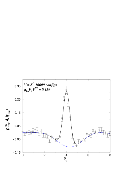
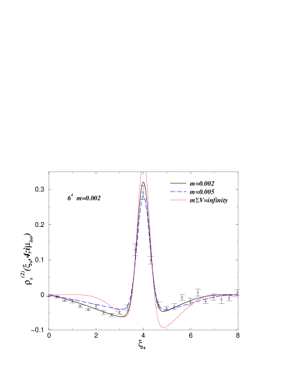
Figure 13: Quenched [55] (left) and unquenched [56] (right) Lattice data at $V=8^{4}$ (left) and $\alpha=0.152$ at $V=6^{4}$ (right), vs. the connected correlation $\rho_{S\ (1,1)}^{(N_{f},\nu)\ conn}(\xi,\zeta)$ (see eq. (6.21) for quenched).

In fig. 13 left the quenched connected $\rho_{S\ (1,1)}^{(N_{f},\nu)\ conn}(\xi,\zeta)$ density eq. (6.21) is plotted versus lattice data [55]: here the second argument is kept fixed at $\zeta=4$ while the first argument $\xi$ is varied. For comparison the same correlation function in the limit $\mu\to 0$ is inserted in dashed line, omitting the delta-spike at $\xi=\zeta=4$.

In the second plot fig. 13 right the unquenched density generalising eq. (6.21) (see [56, 62] for details) is compared to the data. The data nicely fit the curve corresponding to bare mass $m=0.002$ (lowest curve to the left), distinguishing well from the parameter set inserted for comparison $m=0.005$ (see [56] for the corresponding simulations). The quenched limit obtained by setting $2Nm=\infty$ is inserted for comparison as well (lowest curve on the right). This example underlines once more the fruitful interplay between MMs, effective field theory and Lattice simulations.

7 Conclusions and Open Problems

We have seen that Matrix Models are a useful tool to investigate QCD with both real and imaginary chemical potential, extending their previous success for zero $T$ and zero $\mu$. MMs provide both qualitative predictions such as for the phase diagram, and quantitative results for the Dirac operator spectrum that can be confronted with Lattice simulations.

Following the symmetry classification into 3 classes we have explicitly shown how to construct and solve MMs with complex eigenvalues for two of these 3 classes, the class with three or more colours $N_{C}\geq 3$ containing QCD, and the class of adjoint QCD. All complex eigenvalue correlation functions could be computed for these two classes as a function of the number of quark flavours $N_{f}$, their masses $m_{f}$ and chemical potential of equal modulus $\pm\mu$. In particular this included unquenched correlation functions in QCD where the spectral densities become complex valued quantities.

The same construction was then repeated to build a MM for the QCD class with imaginary isospin chemical potential. Here all real eigenvalues correlation functions were computed for the two sets of Dirac operators $\hbox to0.0pt{ $\,\raisebox{0.6458pt}{/}\hss$}D(\pm i\mu)$.

Several issues have been understood on the way. The equivalence with the underlying effective field theory, the epsilon regime of chiral perturbation theory was shown for the QCD class both for real and imaginary $\mu$, on the level of the partition function for an arbitrary set of chemical potentials $\mu_{f}$. We have seen for QCD why the partition function with ordinary quarks and the corresponding sum rules remain $\mu$-independent, while the generating functional for the density is $\mu$-dependent. The strong oscillations and the complex nature of the unquenched eigenvalue density in QCD have been made responsible for chiral symmetry breaking, in contrast to quenched and phase quenched QCD.

The detailed MM predictions for the microscopic density explained the different signatures of complex Dirac eigenvalues, including their attraction or repulsion from the real and imaginary axis. Excellent agreement was found when comparing these quantitatively to Lattice simulations. We made comparisons to quenched QCD using staggered and overlap fermions, allowing to compare to different topological sectors of the gauge fields. For the adjoint QCD class we could compare to unquenched simulations. Here staggered fermions with two colours and fermions in the fundamental representation were used, which are in the same symmetry class. Again excellent agreement was found when lowering the mass to effectively unquenched the eigenvalues close to the origin.

For imaginary isospin chemical potential in the QCD class we could make the same comparison between analytic predictions for two Dirac operators with different real eigenvalues and Lattice data using staggered fermions. Both for quenching and unquenching an excellent agreement was found.

Several interesting problems remain open within the MM approach. Fortunately the symmetry class including unquenched QCD is technically the simplest within MMs. Nevertheless partially quenched correlation functions with several different $\mu_{f}$ have so far only been computed for imaginary chemical potential for 2 flavours, $\mu_{1}\neq\mu_{2}$. It would be very interesting to extend this to more flavours, and in particular to real $\mu$, allowing for instance to compute correlations with $\hbox to0.0pt{ $\,\raisebox{0.6458pt}{/}\hss$}D(\mu_{f})$ in a background of zero chemical potential.

To match with the partially quenched $\chi$PT we would have to compute the corresponding group integral for a general baryon charge matrix $B$. Although we have shown that the expression for MMs and $\chi$PT are equal, we have not yet been able to compute the integral in either way.

Turning to the 2 other symmetry classes only the class for adjoint QCD corresponding to symplectic MMs has bee completely solved. Here the link to $\epsilon\chi$PT is an open question for $N_{f}>2$. The $\beta_{D}=1$ class for two-colour QCD remains the most challenging problem for MMs. Even the easier corresponding non-chiral model of real non-symmetric matrices has resisted a solution for 40 years. This class would be very interesting also from a Lattice perspective as it has a sign problem: although the determinant $\det[\hbox to0.0pt{ $\,\raisebox{0.6458pt}{/}\hss$}D(\mu)+m]$ remains real its sign fluctuates.

Lattice simulations of these 2 latter classes may now be feasible with chiral fermions at non-vanishing $\mu$ due to the existence of the corresponding overlap Dirac operator at $\beta_{D}=2$, without having to use the staggered formulation. Such simulations would be very interesting to perform. The most exciting challenge of course remains to see the MM for unquenched QCD realised on the Lattice.

As a final remark it is well known that a much larger class of MMs with complex eigenvalues exists, compared to the 3 chiral classes for $\mu=0$. It would be very interesting to identify and solve some of the other classes that may be relevant in wider applications as well.

Acknowledgements: I would like to thank E. Bittner, Y. Fyodorov, E. Kanzieper, M. Lombardo, H. Markum, J. Osborn, A. Pottier, R. Pullirsch, L. Shifrin, G. Vernizzi and T. Wettig for discussions and stimulating collaborations over the past few years, without which this would not have been possible. I am particularly indebted to F. Basile, P. Damgaard, K. Splittorff and J. Verbaarschot for valuable comments on the manuscript. This work is supported by EU network ENRAGE MRTN-CT-2004-005616 and by EPSRC grant EP/D031613/1.

References

- [1] E. V. Shuryak and J. J. M. Verbaarschot, Nucl. Phys. A560 (1993) 306 [hep-th/9212088].
- [2] J. J. M. Verbaarschot and T. Wettig, Ann. Rev. Nucl. Part. Sci. 50 (2000) 343 [hep-ph/0003017].
- [3] T. Guhr, A. Müller-Groeling and H. A. Weidenmüller, Phys. Rep. 299 (1998) 190 [cond-mat/9707301].
- [4] J. J. M. Verbaarschot, Phys. Rev. Lett. 72 (1994) 2531 [hep-th/9401059].
- [5] M. E. Peskin, Nucl. Phys. B175 (1980) 197.
- [6] J. J. M. Verbaarschot and I. Zahed, Phys. Rev. Lett. 73 (1994) 2288 [hep-th/9405005].
- [7] R. J. Szabo, Nucl. Phys. B723 (2005) 163 [hep-th/0504202].
- [8] J. J. M. Verbaarschot, Nucl. Phys. B426 (1994) 559 [hep-th/9401092].
- [9] P. H. Damgaard and S. M. Nishigaki, Nucl. Phys. B518 (1998) 495 [hep-th/9711023].
- [10] T. Wilke, T. Guhr and T. Wettig, Phys. Rev. D57 (1998) 6486 [hep-th/9711057].
- [11] G. Akemann and E. Kanzieper, Phys. Rev. Lett. 85 (2000) 1174 [hep-th/0001188].
- [12] T. Nagao and S.M. Nishigaki, Phys. Rev. D62 (2000) 065007 [hep-th/0003009].
- [13] F. Abild-Pedersen and G. Vernizzi, hep-th/0104028.
- [14] S. M. Nishigaki, P. H. Damgaard and T. Wettig, Phys. Rev. D58 (1998) 087704 [hep-th/9803007]; P. H. Damgaard and S. M. Nishigaki, Phys. Rev. D63 (2001) 045012 [hep-th/0006111].
- [15] M. A. Halasz and J. J. M. Verbaarschot, Phys. Rev. D52 (1995) 2563 [hep-th/9502096].
- [16] H. Leutwyler and A. Smilga, Phys. Rev. D46 (1992) 5607.
- [17] A. Smilga and J. Verbaarschot, Phys. Rev. D51 (1995) 829 [hep-th/9404031].
- [18] J. Gasser and H. Leutwyler, Phys. Lett. B188 (1987) 477.
- [19] J. C. Osborn, D. Toublan and J. J. M. Verbaarschot, Nucl. Phys. B540 (1999) 317 [hep-th/9806110]; P. H. Damgaard, J. C. Osborn, D. Toublan and J. J. M. Verbaarschot, Nucl. Phys. B547 (1999) 305 [hep-th/9811212].
- [20] D. Toublan and J. J. M. Verbaarschot, Nucl. Phys. B603 (2001) 343 [hep-th/0012144].
- [21] G. Akemann and P. H. Damgaard, Phys. Lett. B583 (2004) 199 [hep-th/0311171].
- [22] J. C. Osborn and J. J. M. Verbaarschot, Phys. Rev. Lett. 81 (1998) 268 [hep-ph/9807490]; Nucl. Phys. B525 (1998) 738 [hep-ph/9803419].
- [23] P. H. Damgaard, P. Hernandez, K. Jansen, M. Laine and L. Lellouch, Nucl. Phys. B656 (2003) 226 [hep-lat/0211020].
- [24] M. E. Berbenni-Bitsch, S. Meyer, A. Schäfer, J. J. M. Verbaarschot and T. Wettig, Phys. Rev. Lett. 80 (1998) 1146 [hep-lat/9704018]; M. E. Berbenni-Bitsch, S. Meyer and T. Wettig, Phys. Rev. D58 (1998) 071502 [hep-lat/9804030]; P. H. Damgaard, U. M. Heller and A. Krasnitz, Phys. Lett. B445 (1999) 366 [hep-lat/9810060]. M. Göckeler, H. Hehl, P. E. L. Rakow, A. Schäfer and T. Wettig, Phys. Rev. D59 (1999) 094503 [hep-lat/9811018]. P. H. Damgaard, U. M. Heller, R. Niclasen and K. Rummukainen, Phys. Lett. B495 (2000) 263 [hep-lat/0007041]; P. H. Damgaard, U. M. Heller, R. Niclasen and B. Svetitsky, Nucl. Phys. B633 (2002) 97 [hep-lat/0110028].
- [25] P. Hasenfratz, ’50 Years of Yang-Mills Theory’, ed. G.’t Hooft (World Scientific) [hep-lat/0406033].
- [26] R. G. Edwards , U. M. Heller, J. Kiskis and R. Narayanan, Phys. Rev. Lett. 82 (1999) 4188. [hep-th/9902117]; W. Bietenholz, K. Jansen and S. Shcheredin, JHEP 0307 (2003) 033 [hep-lat/0306022]; L. Giusti, M. Lüscher, P. Weisz and H. Wittig JHEP 0311 (2003) 023 [hep-lat/0309189]; T. DeGrand, Z. Liu and S. Schaefer, Phys. Rev. D74 (2006) 094504, Erratum-ibid. D74 (2006) 099904 [hep-lat/0608019].
- [27] E. Follana, A. Hart, and C. T. H. Davies, Phys. Rev.Lett. 93 (2004) 241601 [hep-lat/0406010]; S. Dürr, C. Hoelbling, and U. Wenger, Phys. Rev. D70 (2004) 094502 [hep-lat/0406027]; K. Y. Wong and R. M. Woloshyn, Phys. Rev. D71 (2005) 094508 [hep-lat/0412001]; E. Follana, A. Hart, C. T. H. Davies and Q. Mason, Phys. Rev. D72 (2005) 054501 [hep-lat/0507011].
- [28] K. Splittorff, PoS (LAT2006) 023 [hep-lat/0610072].
- [29] S. Muroya, A. Nakamura, C. Nonaka, and T. Takaishi, Prog. Theor. Phys. 110 (2003) 615. [hep-lat/0306031].
- [30] C. Schmidt, PoS (LAT2006) 021 [hep-lat/0610116].
- [31] F. Karsch, Plenary talk at Hard Probes 2006, hep-ph/0610024.
- [32] P. de Forcrand and O. Philipsen, PoS (LAT2006) 130 [hep-lat/0611027].
- [33] B. Vanderheyden and A. D. Jackson, Phys. Rev. D64 (2001) 074016 [hep-ph/0102064]; B. Klein, D. Toublan, J. J. M. Verbaarschot, Phys. Rev. D72 (2005) 015007 [hep-ph/0405180].
- [34] J. B. Kogut M. A. Stephanov, D. Toublan, J. J. M. Verbaarschot and A. Zhitnitsky, Nucl. Phys. B582 (2000) 477. [hep-ph/0001171].
- [35] M. A. Stephanov, Phys. Rev. D73 (2006) 094508 [hep-lat/0603014].
- [36] M. A. Halasz, A. D. Jackson and J. J. M. Verbaarschot, Phys. Lett. B395 (1997) 293 [hep-lat/9611008].
- [37] K. Splittorff and J. J. M. Verbaarschot, hep-lat/0609076.
- [38] B. Vanderheyden and A. D. Jackson, Phys. Rev. D62 (2000) 094010 [hep-ph/0003150].
- [39] M. A. Halasz, hep-lat/0011086.
- [40] J. Ambjorn, K. N. Anagnostopoulos, J. Nishimura and J. J. M. Verbaarschot, JHEP 0210 (2002) 062 [hep-lat/0208025].
- [41] Y. V. Fyodorov and H.-J. Sommers, J. Phys. A: Math. Gen. 36 (2003) 3303 [nlin.CD/0207051].
- [42] M. Stephanov, Phys. Rev. Lett. 76 (1996) 4472 [hep-lat/9604003].
- [43] K. B. Efetov, Phys. Rev. Lett. 79, 491 (1997) [cond-mat/9702091]; Phys. Rev. B56, 9630 (1997) [cond-mat/9706055].
- [44] M. L. Mehta, Random Matrices, Second Edition, Academic Press, London 1991.
- [45] M. A. Halasz and J. J. M. Verbaarschot, Phys. Rev. Lett. 74 (1995) 3920 [hep-lat/9501025].
- [46] L. Shifrin and J. J. M. Verbaarschot, Phys. Rev. D73 (2006) 074008 [hep-th/0507220].
- [47] M. A. Halasz, J. C. Osborn and J. J. M. Verbaarschot, Phys. Rev. D56 (1997) 7059 [hep-lat/9704007].
- [48] D. Toublan and J. J. M. Verbaarschot, Nucl. Phys. B560 (1999) 259 [hep-th/9904199].
- [49] A. D. Jackson and J. J. M. Verbaarschot, Phys. Rev. D53 (1996) 7223 [hep-ph/9509324]; T. Wettig, A. Schäfer and H. A. Weidenmüller Phys. Lett. B367 (1996) 28; Erratum-ibid. B374 (1996) 362 [hep-ph/9510258].
- [50] J. C. Osborn, Phys. Rev. Lett. 93 (2004) 222001 [hep-th/0403131]; private communication.
- [51] G. Akemann, Nucl. Phys. B730 (2005) 253 [hep-th/0507156].
- [52] G. Akemann, Phys. Lett. B547 (2002) 100 [hep-th/0206086].
- [53] J. Ginibre, J. Math. Phys. 6 (1965) 440.
- [54] G. Akemann, Y. V. Fyodorov and G. Vernizzi, Nucl. Phys. B694 (2004) 59 [hep-th/0404063].
- [55] P. H. Damgaard, U. M. Heller, K. Splittorff and B. Svetitsky, Phys. Rev. D72 (2005) 091501 [hep-lat/0508029].
- [56] P. H. Damgaard, U. M. Heller, K. Splittorff, B. Svetitsky and D. Toublan, Phys. Rev. D73 (2006) 074023 [hep-lat/0602030]; Phys. Rev. D73 (2006) 105016 [hep-th/0604054].
- [57] J. C. Osborn and T. Wettig, PoS (LAT2005) 200 [hep-lat/0510115].
- [58] J. C. Osborn, PoS (Lat2006) 142, [hep-lat/0610016].
- [59] K. Splittorff and J. J. M. Verbaarschot, Phys. Rev. Lett. 90 (2003) 041601 [cond-mat/0209594]; Nucl. Phys. B683 467 (2004) [hep-th/0310271].
- [60] P. H. Damgaard, Phys. Lett. B425 (1998) 151 [hep-th/9711047].
- [61] M. Luz, Phys. Lett. B643 (2006) 235 [hep-lat/0607022].
- [62] G. Akemann, P. H. Damgaard, J. C. Osborn and K. Splittorff, Nucl. Phys. B to appear, [hep-th/0609059].
- [63] G. Akemann, J. C. Osborn, K. Splittorff and J. J. M. Verbaarschot Nucl. Phys. B712 (2005) 287 [hep-th/0411030].
- [64] K. Splittorff and J. J. M. Verbaarschot, Nucl. Phys. B 757 (2006) 259 [hep-th/0605143].
- [65] M. A. Halasz, A. D. Jackson, R. E. Shrock, M. A. Stephanov and J. J. M. Verbaarschot, Phys. Rev. D58 (98) 096007 [hep-ph/9804290].
- [66] T. Guhr and T. Wettig, Nucl. Phys. B506 (1997) 589 [hep-th/9704055]; B. Seif, T. Wettig and T. Guhr, Nucl. Phys. B548 (1999) 475 [hep-th/9811044].
- [67] B. Klein, D. Toublan and J. J. M. Verbaarschot, Phys. Rev. D68 (2003) 014009 [hep-ph/0301143].
- [68] R. Casalbuoni, hep-ph/0610179; M. Stephanov, PoS (LAT2006) 024 [hep-lat/0701002].
- [69] U. Heller, PoS (LAT2006) 011 [hep-lat/0610114].
- [70] A. V. Smilga and J. Stern, Phys. Lett. B318 (1993) 531.
- [71] T. Banks and A. Casher, Nucl. Phys. B169, 103 (1980).
- [72] A. Zabrodin, Les Houches Lecture Notes, France, 6-25 Jun 2004, hep-th/0412219.
- [73] E. Kanzieper, “Progress in Field Theory Research”, Nova Science, New York 2004 [cond-mat/0312006].
- [74] J. C. Osborn, K. Splittorff and J. J. M. Verbaarschot, Phys. Rev. Lett. 94, 202001 (2005) [hep-th/0501210]; proceedings XQCD in Swansea, August 2005 [hep-lat/0510118].
- [75] Y. V. Fyodorov, B. Khoruzhenko, H.-J. Sommers, Ann. Inst. Henri Poincaré (Physique Theorique) 68 (1998) 449 [chao-dyn/9802025].
- [76] G. Akemann, Phys. Rev. Lett. 89 (2002) 072002 [hep-th/0204068]; J. Phys. A36 (2003) 3363 [hep-th/0204246];
- [77] M.C. Bergère, hep-th/0404126.
- [78] G. Akemann and G. Vernizzi, Nucl. Phys. B660 (2003) 532 [hep-th/0212051].
- [79] Y. V. Fyodorov, B. A. Khoruzhenko and H.-J. Sommers, Phys. Lett. A226 (1997) 46 [cond-mat/9606173]; Phys. Rev. Lett. 79 (1997) 557 [cond-mat/9703152].
- [80] J. J. M. Verbaarschot and I. Zahed, Phys. Rev. Lett. 70 (1993) 3852 [hep-th/9303012].
- [81] K. Splittorff and J. J. M. Verbaarschot, Nucl. Phys. B695 (2004) 84 [hep-th/0402177].
- [82] G. Akemann and F. Basile, Nucl. Phys. B to appear, [math-ph/0606060].
- [83] Y. Sasai, A. Nakamura and T. Takaishi, Nucl. Phys. Proc. Suppl. 129 (2004) 539 [hep-lat/0310046].
- [84] G. Akemann and T. Wettig, Phys. Rev. Lett. 92 (2004) 102002 Erratum-ibid. 96 (2006) 029902 [hep-lat/0308003].
- [85] J. Bloch and T. Wettig, Phys. Rev. Lett. 97, 012003 (2006) [hep-lat/0604020].
- [86] R. Narayanan and H. Neuberger, Nucl. Phys. B443 (1995) 305 [hep-th/9411108]; H. Neuberger, Phys. Lett. B417 (1998) 141 [hep-lat/9707022].
- [87] H. Markum, R. Pullirsch and T. Wettig, Phys. Rev. Lett. 83 (1999) 484 [hep-lat/9906020].
- [88] F. Basile, unpublished.
- [89] E. Kanzieper, J. Phys. A: Math. Gen. 35 (2002) 6631 [cond-mat/0109287].
- [90] G. Akemann, E. Bittner, M.-P. Lombardo, H. Markum and R. Pullirsch, Nucl. Phys. B140 Proc. Suppl. (2005) 568, [hep-lat/0409045].
- [91] G. Akemann and E. Bittner, Phys. Rev. Lett. 96 (2006) 222002 [hep-lat/0603004].
- [92] S. Hands, J. B. Kogut, M.-P. Lombardo, and S. E. Morrison, Nucl. Phys. B558 (1999) 327 [hep-lat/9902034].
- [93] E. Bittner, M.-P. Lombardo, H. Markum and R. Pullirsch, Nucl. Phys. B106 Proc. Suppl. (2002) 468 [hep-lat/0110048].
- [94] T. Guhr and T. Wettig, J. Math. Phys. 37 (1996) 6395 [hep-th/9605110]; A. D. Jackson, M. K. Sener and J. J. M. Verbaarschot, Phys. Lett. B387 (1996) 355. [hep-th/9605183].
- [95] B. Eynard and M. L. Mehta, J. Phys. A 31 (1998) 4449 [cond-mat/9710230].