Gauge-Higgs unification on the brane

Abstract

From the quantum field theory point of view, matter and gauge fields are generally expected to be localised around branes or topological defects occurring in extra dimensions. Here I discuss a simple scenario where, by starting with a five dimensional $SU(3)$ gauge theory, we end up with several 4-D parallel branes with localised “chiral” fermions and gauge fields to them. I will show that it is possible to reproduce the electroweak model confined to a single brane, allowing a simple and geometrical approach to the fermion hierarchy problem. Some nice results of this construction are: Gauge and Higgs fields are unified at the 5-D level; and new particles are predicted: a left-handed neutrino of zero hypercharge, and a massive vector field coupling together the new neutrino to other left-handed leptons.

1 Introduction

In this article I review the talk “Confining the electroweak model to a brane” given during the workshop “The Quest for Unification: Theory Confronts Experiment”, Corfu 2005. I will explain how, by starting with an $SU(3)$ gauge theory defined in a 5-D spacetime, we can end up in the presence of a configuration consisting of several 4-D parallel branes, one of them containing a copy of the electroweak model. Many of the results discussed here can be found in ref. [1]. I have decided to change the title of this review in order to emphasise a result which I consider rather elegant: Some of the components of the original five-dimensional gauge field, which end up localised to the “electroweak brane”, can be identified as the Higgs doublet of the standard model.

To my knowledge, the idea of using extra dimensions to reproduce the Weinberg-Salam model and unify gauge and Higgs fields into a single —more fundamental— field, was first proposed in refs. [2] and [3] by Fairlie and Manton, respectively. Ever since, there have been various attempts to find concrete examples of gauge-Higgs unification [4]-[11]. It has been difficult, however, to reconcile both fields under the same group representation and have them coupled to chiral fermions in the appropriate way. The approach followed here is different from previous works; I first focus in obtaining the correct chiral structure for leptons and quarks of the electroweak model, and then verify that the bosonic degrees coupled to these fermions can be identified with the required Higgs doublet and gauge fields. This is done by picking up fermions with appropriate $SU(2)\times U(1)$ charges from specific $SU(3)$-representations, and then localise them to a 4-D brane.

To confine fermions to a brane, a mechanism proposed by Rubakov and Shaposhnikov [12], is considered. This mechanism is based purely on field theoretical considerations. In their proposal, the wave functions of fermion zero modes concentrate near existing domain walls, generating 4-D massless chiral fermions attached to them (see Fig. 1.a).

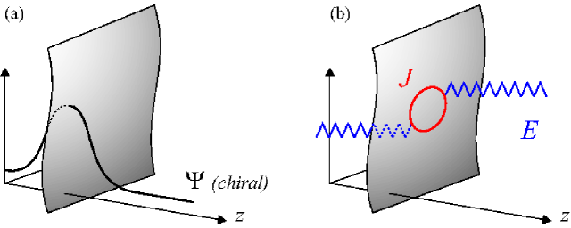
Figure 1: The figures sketch the confinement of fermions and gauge fields to a brane: (a) The wave functions of zero mode fermions are generally found to be localised around domain walls. (b) Gauge fields and other bosonic fields are quasilocalised via loop corrections produced by the zero mode fermions.

As for the gauge fields, a quasilocalisation mechanism proposed by Dvali, Gabadadze and Shifman [16] is taken into account (see refs. [17, 18] for alternative mechanisms). Here, one-loop corrections produced by the interactions between bulk gauge fields and the “already” confined fermions, induce gauge kinetic terms on the brane (see Fig. 1.b). The result is a 4-D effective theory consisting of gauge fields mediating interactions between the confined fermions on the brane.

The key ingredient of the present proposal is that the positions at which 5-D fermions end up localised depend on their $SU(3)$ charges. This allows, for example, to break the $\mathbf{10}$ and $\bar{\mathbf{6}}$ representations of $SU(3)$ down to the lepton and quark representations of $SU(2)\times U(1)$, respectively, and confine them to a single brane. In this construction it is possible to identify the Higgs with the fifth component of the localised gauge field. Additionally, new fields inevitably appear in the resulting 4-D effective theory. These are: a left-handed neutrino with zero-hypercharge, and a massive vector field coupling together the new neutrino to other left-handed leptons.

This article is organised as follows: Section 2 discusses how the confinement of 5-D fermions is produced in the presence of domain walls. Here, a simple toy model consisting of a spin-1/2 fermion coupled to a scalar field through a Yukawa interaction is presented. It is shown that if the scalar field acquires a nontrivial vacuum solution, such as the kink profile, then a zero mode chiral fermion confines about the domain wall. In Section 3 this discussion is extended to include the quasilocalisation of a $U(1)$ gauge field. Then, in Section 4, a more complex and interesting setup is introduced; this time, the bulk fields belong to $SU(3)$ representations. It is shown that the $SU(3)$ gauge symmetry can be broken down by the nontrivial vacuum solutions of charged scalar fields. As a result, depending on the group representation to which bulk fermions belong, several branes form containing different type of matter fields confined to them. In Section 5, we show that the fermions confined in this way have in fact the opportunity to span a representation of $SU(2)_{L}\times U(1)$. This allows the construction of a brane containing leptons and quarks. This analysis is completed in Section 6, where the quasilocalisation of $SU(2)\times U(1)$ gauge fields is considered. Finally, in Section 7, I compare the model obtained in this way with the electroweak sector of the standard model. There I address the fermion hierarchy problem and discuss some relevant phenomenological aspects of the present proposal.

2 Confinement of fermions

Consider a 5-D system consisting of a spin-1/2 fermion $\Psi$ and a real scalar field $\Phi$. To describe the 5-D spacetime we use coordinates $x^{A}$ with $A=1,\ldots,5$. The Lagrangian of the system is

$$\mathcal{L}^{(5)}=-\bar{\Psi}\left[\gamma^{A}\partial_{A}+m+y\,\Phi\right]\Psi-\frac{1}{2}(\partial_{A}\Phi)^{2}-V(\Phi).$$ (1)

Here $m$ is the mass of the bulk fermion $\Psi$ and $y$ is a Yukawa coupling. Additionally, $\gamma^{A}$ are the 5-D gamma-matrices in a basis where

$$\gamma^{5}=\left(\begin{array}[]{cc}1&0\\ 0&-1\end{array}\right),$$ (4)

which is the usual four-dimensional $\gamma^{5}$ matrix. For the time being let us disregard the presence of gauge fields. Consider also the following potential for the scalar $\Phi$

$$V(\Phi)=\frac{\sigma}{4}\left[\Phi^{2}-v^{2}\right]^{2}.$$ (5)

To discuss solutions to this system it is appropriate to use $z=x^{5}$ to distinguish the extra-dimension and coordinates $x^{\mu}$, with $\mu=0,\cdots,3$, to parameterise the usual 4-D spacetime. As well known, the system admits a kink solution for the scalar field $\Phi$, of the form $\Phi(z)=v\tanh\left(kz\right)$, where $k=v\sqrt{\sigma/2}\,$. The corresponding domain wall, centred at $z=0$, is coupled to the fermion field through the $y$-term. Then, the equation of motion for $\Psi$ reads

$$\left[\gamma^{\mu}\partial_{\mu}+\gamma^{5}\partial_{z}+m+y\,\Phi(z)\right]\Psi=0.$$ (6)

Notice that the translational invariance along $z$ is broken. It is therefore useful to define left and right handed helicities $\Psi_{L}$ and $\Psi_{R}$, by $\gamma^{5}\Psi_{L}=+\Psi_{L}$ and $\gamma^{5}\Psi_{R}=-\Psi_{R}$. With this convention in mind, Eq. (6) has two zero mode solutions of the form

$$\Psi_{L,R}=A\exp\Big{\{}\mp\!\int^{z}_{0}\!\!\!\left[m+y\,\Phi(z)\right]\,dz\Big{\}}\,\psi_{L,R}(x),$$ (7)

where $\mp$ stands for left and right handed helicities, respectively, and $\psi_{L}(x)$ and $\psi_{R}(x)$ are 4-D Weyl fermions with opposite chiralities. Additionally, the factor $A$ is a normalisation constant introduced in such a way that

$$\int dz\,|\Psi|^{2}=|\psi(x)|^{2}.$$ (8)

Thus, only one of these two solutions is normalisable: if $y>0$ ($y<0$) then the left (right) handed fermion is normalisable. At this stage, it is convenient to define the following “confinement” length scale:

$$\Delta=\frac{1}{\sqrt{|yvk|}}.$$ (9)

Then, in general, nonzero modes solutions to Eq. (6) provide a tower of states with masses of order $\Delta^{-1}$. From now on I assume that $\Delta$ is sufficiently small so that nonzero modes can be integrated out without affecting the theory at low energies. Additionally, observe that if $m=0$ then the fermion wave function is centred at $z=0$, otherwise its localisation is shifted with respect to the brane. To understand better this, let us analyse the linear behaviour $\Phi\simeq vkz$ near $z=0$ for the case $y>0$. Then, assuming that $m^{-1}\gg k\Delta^{2}$ (so the linear expansion $\Phi\simeq vkz$ makes sense), we obtain

$$\Psi_{L}\sim\frac{1}{\sqrt{\Delta}}\exp\left[-\frac{1}{2}\Delta^{-2}(z-z_{0})^{2}\right]\,\psi_{L}(x),$$ (10)

where $z_{0}=-m\Delta^{2}$. Thus, the fermion wave function has a width $\Delta$ and is centred at $z_{0}$ (see Fig. 2).

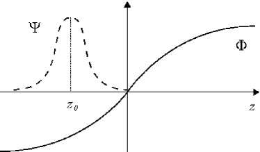
Figure 2: The figure sketches the confinement of the bulk fermion near the domain wall located at $z=0$. The fermion wave function is centred at position $z_{0}=-m\Delta^{2}$.

It should be noticed that the width $\Delta$ of the fermion wall is not necessarily related to the width of the domain wall produced by the scalar, which, here, is of order $k^{-1}$. We can now compute the 4-D effective Lagrangian for $\psi_{L}(x)$ by integrating out the extra-dimension:

$$\mathcal{L}^{(4)}=-\bar{\psi}_{L}(\gamma^{\mu}\partial_{\mu})\psi_{L}.$$ (11)

Notice that in the limit $\Delta\rightarrow 0$ ($z_{0}\rightarrow 0$), we obtain a thin brane characterised by

$$\mathcal{L}^{(5)}=\delta(z)\mathcal{L}^{(4)}.$$ (12)

There is an interesting consequence related to the shift of the fermion’s positions with respect to the domain wall: Suppose a scenario in which two bulk fermions $\Psi^{1}$ and $\Psi^{2}$, with masses $m_{1}$ and $m_{2}$, are coupled to a wall in such a way that $y_{1}=y>0$ and $y_{2}=-y<0$. If in the original 5-D Lagrangian there is a term such as $H\bar{\Psi}^{1}\Psi^{2}+\mathrm{h.c.}$, where $H$ is a given bulk field (a scalar, for example), then the 4-D effective Lagrangian will contain a Yukawa term of the form

$$\sim(H\,\bar{\psi}^{1}_{L}\,\psi^{2}_{R}+\mathrm{h.c.})\,e^{-r^{2}/4\Delta^{2}},$$ (13)

where $r=r_{1}-r_{2}$ is the separation between both fermion wave functions with $r_{1}=-m_{1}\Delta^{2}$ and $r_{2}=+m_{2}\Delta^{2}$. This means a mechanism to exponentially suppress 4-D Yukawa couplings [in this case, for the pair ($\psi^{1}_{L}$, $\psi^{2}_{R}$)]. This is the basis for the split fermion scenario [13, 14, 15]. I will come back to this mechanism in Section 7, where the fermion hierarchy problem is addressed.

3 Quasilocalisation of gauge fields

Gauge fields can be found localised to a brane with the help of the already confined fermions. In the case of the quasilocalisation of gauge fields [16], the interaction between the fermionic currents at the branes and the 5-D gauge fields induces a 4-D effective theory. This is produced by one-loop contributions to the effective action on the brane (see ref. [19] for the case of gravity). Consider, for instance, the same setup as before but now in the presence of a $U(1)$ gauge field $E_{A}$ with a gauge coupling $g$. This time the Lagrangian reads

$$\mathcal{L}^{(5)}=-\bar{\Psi}\gamma^{A}(\partial_{A}-iE_{A})\Psi-\frac{1}{4g^{2}}F_{AB}F^{AB}+\mathcal{L}(\Phi),$$ (14)

where $\mathcal{L}(\Phi)$ is the Lagrangian for the scalar field $\Phi$, and $F_{AB}=\partial_{A}E_{B}-\partial_{B}E_{A}$ is the gauge antisymmetric tensor. Then, after the fermion confines to the wall produced by $\Phi$, in the thin wall approximation $\Delta\rightarrow 0$, the gauge sector appears having the following Lagrangian

$$\mathcal{L}^{(5)}_{\mathrm{G}}=-\frac{1}{4g^{2}}F_{AB}F^{AB}+\delta(z)E_{\mu}J^{\mu}(x).$$ (15)

The current term $J^{\mu}(x)=i\bar{\psi}_{L}\gamma^{\mu}\psi_{L}$, localised to the brane, appears as a consequence of the covariant derivative $D_{A}\Psi=(\partial_{A}-iE_{A})\Psi$. (The scalar component $E_{5}$ plays no role here because it couples $\psi_{L}$ to the non-normalisable piece $\Psi_{R}$). Then, a one-loop correction induces the following Lagrangian for $E_{\mu}$ on the brane

$$\mathcal{L}^{(4)}=-\frac{1}{4\lambda^{2}}F_{\mu\nu}F^{\mu\nu},\qquad\lambda^{-2}=\frac{N}{12\pi^{2}}\ln(\Lambda/\mu),$$ (16)

where $F_{\mu\nu}=\partial_{\mu}E_{\nu}-\partial_{\nu}E_{\mu}$ is the antisymmetric tensor for the 4-D sector $E_{\mu}$. Here, $\Lambda$ and $\mu$ are the ultraviolet and infrared cut-offs scales of the 5-D theory and $N$ is the number of such fermions $\psi_{L}$ participating in the loops. As a consequence, the five-dimensional theory describing the gauge sector near the brane, is found to have the form

$$\mathcal{L}^{(5)}=-\frac{1}{4g^{2}}F_{AB}F^{AB}-\delta(z)\frac{1}{4\lambda^{2}}F_{\mu\nu}F^{\mu\nu}.$$ (17)

Notice that $g^{2}$ is a dimensionful quantity, whereas $\lambda$ is dimensionless. In fact, if the propagation of gauge bosons in this theory is studied, one finds that there is a crossover scale $r_{c}=g^{2}/2\lambda^{2}$. At distances bellow this scale, the fields propagate along the brane, whereas at larger distances, the gauge bosons start spreading out of the brane (see Fig. 3).

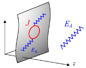
Figure 3: The figure represents the propagation of gauge fields in the bulk and the brane. If the field’s wavelength is smaller than $r_{c}$, its propagation is dominated by loop corrections taking place on the brane, and becomes well localised.

4 Confining $SU(3)$ fermions

The toy model presented in Section 2 provided a useful description of how fermions can end up localised around a domain wall produced by the non trivial vacuum solution of a scalar field. It is possible to find more interesting phenomena by including a non-Abelian gauge symmetry. For example, if the fields generating the walls are gauge-charged, then the fermions confined to these walls have the chance of inheriting interesting properties coming from the original symmetry. In this section we analyse a simple case involving a five-dimensional $SU(3)$ gauge theory. To start, assume that spacetime is described by a 5-D manifold $M$ with topology

$$M=\mathbb{R}^{4}\times S^{1},$$ (18)

where $S^{1}$ is the one-dimensional circle and $\mathbb{R}^{4}$ is the 4-D Lorentzian space. In this case, the coordinate $z=x^{5}\in[0,L]$ is the spatial coordinate parameterising $S^{1}$ with $L$ the size of the compact extra-dimension. Let us consider the existence of 5-D bulk fermions transforming nontrivially under $SU(3)$ gauge symmetry. They are described by the following Lagrangian

$$\mathcal{L}_{\Psi}^{(5)}=-\bar{\Psi}[\gamma^{A}D_{A}+Y(\Phi)]\Psi.$$ (19)

The covariant derivative is $D_{A}\Psi=(\partial_{A}-iE^{\alpha}_{A}T_{\alpha})\Psi$, where $E^{\alpha}_{A}$ are $SU(3)$ bulk gauge fields. Here $\alpha=1,\ldots,8$ and $T_{\alpha}$ are the $SU(3)$ generators acting on $\Psi$. Observe that there is a coupling term $Y(\Phi)$ where $\Phi=\Phi^{\alpha}T_{\alpha}$ is a scalar field that transforms in the adjoint representation of $SU(3)$. In order to construct $SU(3)$-representations we can proceed conventionally: We choose $T_{3}$ and $T_{8}$ as the Cartan generators and construct states to be eigenvalues with charges $Q=(T_{3},T_{8})$. To continue, assume that $\Phi$ is dominated by the following $SU(3)$ gauge invariant potential

$$V(\Phi)=\frac{\sigma}{4}\left[\Phi^{\alpha}\Phi_{\alpha}-v^{2}\right]^{2}.$$ (20)

Nonzero vacuum expectation solutions $\langle\Phi\rangle$ are expected and, in general, they correspond to linear combinations of $\langle\Phi^{3}\rangle$ and $\langle\Phi^{8}\rangle$. Furthermore, since the compact topology (18) has been assumed, the system admits nontrivial topological solutions. Take for instance the case of a single winding-number solution

$$\langle\Phi(z)\rangle=\Phi_{0}\left[\cos(kz)T_{3}+\sin(kz)T_{8}\right],$$ (21)

where $k=2\pi/L$ and $\Phi_{0}^{2}=v^{2}-k^{2}/\sigma$. Notice that $\langle\Phi^{8}\rangle=0$ at $z=0$. This solution allows to parameterise the extra-dimension in terms of $\Phi^{3}$ and $\Phi^{8}$ values (see Fig. 4.a). We can now proceed in the same way as in Section 2: By defining left and right handed fermions $\Psi_{L}$ and $\Psi_{R}$, it is possible to find zero mode solutions of the form

$$\Psi_{L,R}=A\exp\left\{\mp\int^{z}_{0}\!\!\!Y(z)\,dz\right\}\,\psi_{L,R}(x),$$ (22)

where $Y(z)\equiv Y[\langle\Phi(z)\rangle]$. In general, given a nonzero v.e.v for a scalar field $\Phi(z)$, the position $z$ at which the fermion wave function $\Psi$ is centred is determined by the condition $Y(z)\,\Psi=0$ (See Fig. 4.b). The chirality of such a state is determined by the sign of the derivative $\partial_{z}Y(\Phi)$ at the given position. To be more precise, if $\partial_{z}Y(\Phi)>0$ ($\partial_{z}Y(\Phi)<0$), then the confined fermion is left (right) handed.

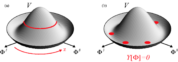
Figure 4: The potential $V(\Phi)$ in terms of the scalar components $\Phi^{3}$ and $\Phi^{8}$. (a) The loop around the hill describes the single winding-number solution. Observe that it is possible to parameterise the coordinate $z$ in terms of $\Phi$-values. (b) The positions at which chiral fermions end up confined can be deduced from the condition $Y[\Phi]=0$.

To discuss the consequences of solution (21) with some transparency, let us have a look at the following simple example: Consider a Yukawa coupling of the form

$$Y(\Phi)=y\Phi=y\Phi^{\alpha}T_{\alpha},$$ (23)

and matter fields $\Psi$ belonging to the $\mathbf{3}$, the fundamental representation of $SU(3)$. In this case the confinement length scale must be defined as $\Delta=|y\Phi_{0}k|^{-1/2}$. Thus again, the masses of nonzero mode states are found to be of order $\Delta^{-1}$. To work out the consequences of the Yukawa coupling (23) on the $\mathbf{3}$, it is convenient to choose $\Psi^{i}$ (with $i=1,2,3$) to have the following $SU(3)$ charges (see Fig. 5):

$$Q(\Psi^{1})=(-1/2,+\sqrt{3}/6),\qquad Q(\Psi^{2})=(+1/2,+\sqrt{3}/6),\qquad Q(\Psi^{3})=(0,-\sqrt{3}/3).$$ (24)

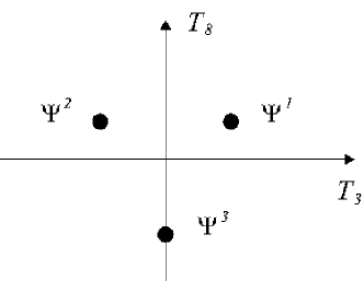
Figure 5: The figure shows the $SU(3)$ charges $Q=(T_{3},T_{8})$ of fermions $\Psi^{i}$ (with $i=1,2,3$) in the fundamental representation $\mathbf{3}$.

In this way, replacing (23) into (22), it is possible to see that the positions at which the fermion wave functions end up centred depend on their $SU(3)$ charges and their chiralities. Observe, for instance, that in the present realisation left and right-handed fermions are localised to diametrically opposite positions in the $S^{1}$ circle. The respective positions are: $z=0$ for $\Psi^{3}_{R}$, $z=L/2$ for $\Psi^{3}_{L}$, $z=2L/3$ for $\Psi^{1}_{R}$, $z=L/6$ for $\Psi^{1}_{L}$, $z=5L/6$ for $\Psi^{2}_{R}$, and $z=L/3$ for $\Psi^{2}_{L}$. Also, it can be seen that if $|y\Phi_{0}|\gg k$, then the widths of wave functions become of order $\Delta$ and the overlap between fermions located at different positions becomes very small. Thus, the fundamental representation has been broken down to several branes. Figure 6 shows the way in which $\Psi^{3}$ of the fundamental representation is split.

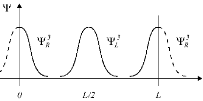
Figure 6: The figure shows the way in which $\Psi^{3}$ is confined. Same representations but with different chiralities end up in branes located at diametrically opposite positions in the $S^{1}$ circle.

Now it is possible to compute the 4-D effective theory for the matter fields localised at any desired brane of our example. Let us compute, for instance, the effective Lagrangian $\mathcal{L}_{\mathrm{eff}}$ at the first brane ($z=0$) taking into account the presence of the gauge field $E^{\alpha}_{A}$. In the limit $\Delta\rightarrow 0$ with $L$ fixed, the following expression is obtained

$$\mathcal{L}_{\mathrm{eff}}=-\delta(z)\bar{\psi}^{3}_{R}\gamma^{\mu}\bigg{[}\partial_{\mu}+i\frac{\sqrt{3}}{3}E^{8}_{\mu}\bigg{]}\psi^{3}_{R}.$$ (25)

Here the delta function appears in the limit $\Delta\rightarrow 0$ after considering the right normalisation factor $A$ in Eq. (22). Notice the appearance of the induced current

$$J_{8}^{\mu}=-i\frac{\sqrt{3}}{3}\bar{\psi}^{3}_{R}\gamma^{\mu}\psi^{3}_{R},$$ (26)

which couples to the gauge field component $E^{8}_{\mu}$ in (25). Then, as discussed in Section 3, a one-loop correction induces the following Lagrangian for $E^{8}_{\mu}$ at the brane

$$\mathcal{L}^{(4)}=-\frac{1}{4\lambda^{2}}(\partial_{\mu}E^{8}_{\nu}-\partial_{\nu}E^{8}_{\mu})^{2},\qquad\lambda^{-2}=\frac{N}{12\pi^{2}}\ln(\Lambda/\mu).$$ (27)

Here $N=1/3$, which comes from the coefficient $\sqrt{3}/3$ in $J_{8}^{\mu}$. The final theory confined to $z=0$ corresponds to a $U(1)$ gauge theory.

5 Confining the electroweak model to a brane

We now turn to the confinement of the electroweak model. Our approach consists of adding a new scalar field into the model so as to allow a richer structure to the localisation mechanism generated by the $Y$-coupling. Then we show that leptons can be obtained from the $\mathbf{10}$-representation of $SU(3)$, while quarks can be obtained from the $\mathbf{\bar{6}}$. To start, assume the existence of the same scalar field $\Phi=\Phi^{\alpha}T_{\alpha}$ (as discussed previously) and an additional scalar field $\Theta=\Theta^{\alpha}T_{\alpha}$ also transforming in the adjoint representation of $SU(3)$. The dynamics of this scalar is dominated by the following $SU(3)$ gauge invariant potential

$$U\propto\left[\Theta^{\alpha}\Theta_{\alpha}-u^{2}\right]^{2},$$ (28)

where $u$ is a constant parameter of the theory. Now, consider the following $Y$-coupling:

$$Y=-y\left(\frac{1}{2}\{\Phi,\Theta\}-\frac{1}{4}\Theta^{\alpha}\Phi_{\alpha}+p\frac{\sqrt{3}}{2}u\,\Phi\right),$$ (29)

where $\{\,,\}$ denotes anticommutation. In the previous equation, $p$ is a parameter of the model that depends on the representation on which $Y$ is acting; in the present construction $p=1$ if $Y$ couples to the $\mathbf{10}$, and $p=-1/3$ if $Y$ couples to the $\mathbf{\bar{6}}$. Other gauge invariant terms can also be included in (29) without modifying the main results of this section (I will come back to this in Section 7).

Let us focus on the case in which $\Theta$ acquires the following vacuum expectation value (v.e.v.) $\langle\Theta\rangle=u\,T_{8}$. This particular value could be due, for example, to a small contribution $\propto\Tr\Theta^{4}$ to the potential $U$ of Eq. (28). Then, after the scalars have acquired their respective v.e.v.’s we are left with the following $z$-dependent coupling

$$(y\Phi_{0}u)^{-1}Y=-\left[(T_{8}+p\sqrt{3}/2)T_{8}-1/4\right]\sin(kz)-\left[T_{8}+p\sqrt{3}/2\right]T_{3}\cos(kz).$$ (30)

Similar to our previous example, in this case the widths of the fermion wave functions become of order $\Delta$, the confining length scale, which now is found to be $\Delta=|y\Phi_{0}uk|^{-1/2}$. In what follows I analyse separately the confinement of leptons (from the $\mathbf{10}$) and quarks (from the $\mathbf{\bar{6}}$).

5.1 Leptons

Here I study the action of $Y$ on the $\mathbf{10}$ (where $p=1$) and show that the confined fermions to the domain wall can be identified with the usual leptons of the electroweak model. To proceed it is convenient to consider the decomposition of $SU(3)$ into $SU(2)$ subgroups (see Fig. 7.a).

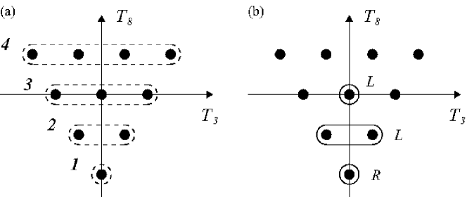
Figure 7: (a) The $\mathbf{10}$ representation and its decomposition into $SU(2)$ subgroups: this is $\mathbf{10}=\mathbf{1}\oplus\mathbf{2}\oplus\mathbf{3}\oplus\mathbf{4}$ with charges $T_{8}=-\sqrt{3},-\sqrt{3}/2,\,0,+\sqrt{3}/2$, respectively. (b) States of the $\mathbf{10}$ that end up localised to $z=0$. The labels $L$ and $R$ indicate the chirality of the confined states.

The $\mathbf{10}$ has the following decomposition: $\mathbf{10}=\mathbf{1}\oplus\mathbf{2}\oplus\mathbf{3}\oplus\mathbf{4}$, with the following $T_{8}$-charges: $T_{8}=-\sqrt{3},-\sqrt{3}/2,\,0,+\sqrt{3}/2$. Using this notation, the localisation produced by the $Y$-coupling to the first brane at $z=0$ can be worked out. First, observe from Eq. (30) that all of those states in the $\mathbf{10}$ with $(T_{8}+\sqrt{3}/2)T_{3}=0$ result in $Y=0$ at $z=0$. Then, following the reasoning of Section 4, a chiral fermion from each one of these states confine to $z=0$. The precise chirality of each state depends on the sign of $\partial_{z}Y(z)$. In the present case, assuming $y>0$, the confined states are: The right-handed $SU(2)$-singlet $R\equiv\psi^{\mathbf{1}}_{R}$ with charge $Q=(0,-\sqrt{3})$; the two left-handed components of the $SU(2)$-doublet $L\equiv\psi^{\mathbf{2}}_{L}$ with charges $Q=(-1/2,-\sqrt{3}/2)$ and $Q=(+1/2,-\sqrt{3}/2)$; and only one left-handed component from the triplet $N\equiv\psi^{\mathbf{3}}_{L}$, with charge $Q=(0,0)$. States with opposite chirality are confined to a “mirror-brane” located at $z=L/2$, and any other state confines elsewhere. Figure 7.b shows those components of the $\mathbf{10}$ that confine to $z=0$.

5.2 Quarks

The case for quarks is very similar. Here, the value $p=-1/3$ in the $Y$-coupling (30) needs to be considered. Having said this, recall that the $\mathbf{\bar{6}}$ can be decomposed into $\mathbf{\bar{6}}=\mathbf{1}\oplus\mathbf{2}\oplus\mathbf{3}$ with the following $T_{8}$ charges: $T_{8}=+2\sqrt{3}/3,+\sqrt{3}/6,-\sqrt{3}/3$ (see Fig. 8.a).

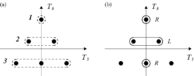
Figure 8: (a) The $\mathbf{\bar{6}}$ representation and its decomposition into $SU(2)$ subgroups: this is $\mathbf{\bar{6}}=\mathbf{1}\oplus\mathbf{2}\oplus\mathbf{3}$ with charges $T_{8}=+2\sqrt{3}/3,+\sqrt{3}/6,-\sqrt{3}/3$ respectively. (b) States of the $\mathbf{\bar{6}}$ that end up localised to $z=0$. The labels $L$ and $R$ indicate the chirality of the confined states.

Then, the following four chiral states are found to be confined: The right-handed $SU(2)$-singlet $\psi_{R}^{\mathbf{1}}$ with charge $Q=(0,+2/\sqrt{3})$; the two left-handed components of the $SU(2)$-doublet $\psi_{L}^{\mathbf{2}}$ with charges $Q=(-1/2,+1/2\sqrt{3})$ and $Q=(+1/2,+1/2\sqrt{3})$; and only one right-handed component from the triplet $\psi_{L}^{\mathbf{3}}$, with charge $Q=(0,-1/\sqrt{3})$. Figure 8.b shows those components of the $\mathbf{\bar{6}}$ that confine to $z=0$. These states have the appropriate quantum numbers for this sector to be identified with the quarks of the standard model.

5.3 Effective theory

We can now be more explicit by computing the effective theory for the states confined to the brane at $z=0$. Let us analyse, for instance, the case for leptons. To this extent, consider the following decomposition of the five-dimensional $SU(3)$ gauge field $E^{\alpha}_{A}$:

$$W_{\mu}^{a} = E_{\mu}^{a}\qquad\mathrm{with}\qquad a=1,2,3,$$ (31)

$$V_{\mu}^{i} = E_{\mu}^{i}\qquad\mathrm{with}\qquad i=4,5,6,7,$$ (32)

$$\phi^{i} = E_{5}^{i}\qquad\mathrm{with}\qquad i=4,5,6,7,$$ (33)

$$B_{\mu} = E_{\mu}^{8}.$$ (34)

In the limit $\Delta\rightarrow 0$, other components of $E_{A}^{\alpha}$ are decoupled from the matter fields confined to the brane (this is because these components are coupling together spinor fields with different chiralities that necessarily end up at different branes). In this decomposition, the only nonzero structure constant are: $C_{ab}^{c}$, $C_{ij}^{a}$ and $C_{ij}^{8}$ (and obvious permutation of indices). Then, in the thin wall approximation, the 4-D effective Lagrangian for the massless leptons at the first brane is found to be

$$\mathcal{L}_{\mathrm{lep}}^{(4)}=-\bar{L}\Big{[}\gamma^{\mu}\partial_{\mu}-i\gamma^{\mu}W^{a}_{\mu}T_{a}+i\frac{\sqrt{3}}{2}\gamma^{\mu}B_{\mu}\Big{]}L-\bar{R}\Big{[}\gamma^{\mu}\partial_{\mu}+i\sqrt{3}\gamma^{\mu}B_{\mu}\Big{]}R-\bar{N}\gamma^{\mu}\partial_{\mu}N+\mathcal{L}_{\mathrm{I}}^{(4)},\quad$$ (35)

where $\mathcal{L}_{\mathrm{I}}^{(4)}$ contains interaction terms involving $\phi^{i}$ and $V^{i}_{\mu}$

$$\mathcal{L}_{\mathrm{I}}^{(4)}=-i\alpha\frac{\sqrt{3}}{2}\phi^{i}\bar{R}\,t_{i}\,L-i\beta V^{i}_{\mu}\bar{N}\gamma^{\mu}\,s_{i}\,L+\mathrm{h.c.},$$ (36)

with $\alpha$ and $\beta$ coefficients emerging from the overlap between wave functions of different widths. In the present case, $\alpha=\beta=(5)^{1/4}/\sqrt{3}$. Additionally, $t_{i}$ and $s_{i}$ with $i=4,5,6,7$, are $1\times 2$ matrices acting on the $SU(2)$ doublet $L$ given by

$$t_{4}=s_{6}=(1,0),\qquad t_{5}=-s_{7}=i(1,0),\qquad t_{6}=s_{4}=(0,1),\qquad t_{7}=-s_{5}=i(0,1).$$ (37)

These matrices appear as a consequence of the action of the operators $T_{i}$’s on those states of the $\mathbf{10}$ that are later identified with $L$.

5.4 About the other branes

To finish, let us briefly mention that other branes are also formed in the bulk. They appear from the localisation of the rest of the states of the $\mathbf{\bar{6}}$ and $\mathbf{10}$ representations. The most interesting brane is the “mirror brane” at $z=L/2$, which contains a copy of the electroweak model obtained at the first brane $z=0$, but with states having opposite chiralities. The rest of the branes (also determined by the condition $Y=0$) all contain different versions of $U(1)$ Abelian gauge theories (see Fig. 9).

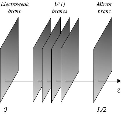
Figure 9: The figure sketches the disposition of branes in the 5-D bulk. The electroweak brane is located at $z=0$, while the mirror brane (a copy of the first brane but containing matter with opposite chirality) is located at $z=L/2$.

6 Localisation of $SU(2)\times U(1)$ gauge fields

The effective theory of Eq. (35) is invariant under $SU(2)\times U(1)$ gauge symmetry. Before fully identifying this theory with the electroweak model in Section 7, it is important to consider the localisation of the gauge fields $W^{a}_{\mu}$, $B_{\mu}$, $\phi^{i}$ and $V_{\mu}^{i}$ to the brane. To start, observe that there is an $SU(2)\times U(1)$ current term attached to the brane of the form

$$E^{\alpha}_{A}J^{A}_{\alpha}=W^{a}_{\mu}J_{a}^{\mu}(x)+B_{\mu}J^{\mu}(x)+V^{i}_{\mu}J_{i}^{\mu}(x)+\phi^{i}J_{i}(x).$$ (38)

Since the effective terms for gauge fields are induced by loop corrections from these currents, the transformation properties of $J^{A}_{\alpha}(x)$ are transferred to the quasilocalised gauge fields. Therefore, the 4-D induced action for $W_{\mu}^{a}$, $V_{\mu}^{i}$, $B_{\mu}$ and $\phi^{i}$ at the first brane ($z=0$) becomes

$$\mathcal{L}^{(4)}_{\mathrm{G}}=-\frac{1}{4\lambda^{2}_{H}}H^{a}_{\mu\nu}H_{a}^{\mu\nu}-\frac{1}{4\lambda^{2}_{G}}G_{\mu\nu}G^{\mu\nu}-\frac{1}{2\lambda^{2}_{\phi}}|D\phi|^{2}-\frac{1}{4\lambda^{2}_{Q}}Q^{i}_{\mu\nu}Q_{i}^{\mu\nu}+\mathcal{L}_{V}.$$ (39)

Here $H_{\mu\nu}^{a}$, $Q_{\mu\nu}^{i}$, $G_{\mu\nu}$ and $D_{\mu}\phi^{i}$ are defined as

$$H_{\mu\nu}^{a} = \partial_{\mu}W_{\nu}^{a}-\partial_{\nu}W_{\mu}^{a}+C^{a}_{bc}W_{\mu}^{b}W_{\nu}^{c},$$

$$Q_{\mu\nu}^{i} = \partial_{\mu}V_{\nu}^{i}-\partial_{\nu}V_{\mu}^{i}+C^{i}_{aj}W_{\mu}^{a}V_{\nu}^{j}+C^{i}_{ja}V_{\mu}^{j}W_{\nu}^{a}+C^{i}_{8j}B_{\mu}V_{\nu}^{j}+C^{i}_{j8}V_{\mu}^{j}B_{\nu},$$

$$G_{\mu\nu} = \partial_{\mu}B_{\nu}-\partial_{\nu}B_{\mu},$$

$$D_{\mu}\phi^{i} = \partial_{\mu}\phi^{i}+C^{i}_{aj}W^{a}_{\mu}\phi^{j}+C^{i}_{8j}B_{\mu}\phi^{j}.$$ (40)

Additionally, in Eq. (39) there is $\mathcal{L}_{V}$, which contains interaction terms between the vector field $V_{\mu}^{i}$ and the rest of the induced fields

$$\mathcal{L}_{V}=-\frac{1}{4\lambda^{2}_{1}}\left(R_{\mu\nu}^{a}R^{\mu\nu}_{a}+K_{\mu\nu}K^{\mu\nu}\right)-\frac{1}{2\lambda^{2}_{2}}H^{a}_{\mu\nu}R^{\mu\nu}_{a}-\frac{1}{2\lambda^{2}_{3}}G_{\mu\nu}K^{\mu\nu}-\frac{1}{2\lambda^{2}_{4}}\left(S_{\mu}^{a}S^{\mu}_{a}+S_{\mu}S^{\mu}\right),$$ (41)

where we have defined: $R_{\mu\nu}^{a}=C^{a}_{ij}V_{\mu}^{i}V_{\nu}^{j}$, $S_{\mu}^{a}=C^{a}_{ij}V_{\mu}^{i}\phi^{j}$, $S_{\mu}=C_{ij}^{8}V^{i}_{\mu}\phi^{j}/\sqrt{3}$ and $K_{\mu\nu}=C^{8}_{ij}V_{\mu}^{i}V_{\nu}^{j}/\sqrt{3}$. Finally, the various couplings $\lambda_{H}$, $\lambda_{G}$, $\lambda_{Q}$ and $\lambda_{\phi}$ in (39), and $\lambda_{1}$, $\lambda_{2}$, $\lambda_{3}$ and $\lambda_{4}$ in (41) are, in general, found to be of the form

$$\frac{1}{\lambda^{2}}=\frac{N}{12\pi^{2}}\ln\frac{\Lambda}{\mu},$$ (42)

where $N$ measures the number of fermions present in the different loops, taking also into account the values of the various $SU(3)$-charges and combinatorics. For example, we have

$$N_{H}=\mathrm{Tr}\left(T_{3}^{2}\right),\quad\mathrm{and}\quad N_{G}=\mathrm{Tr}\left(T_{8}^{2}\right),$$ (43)

where the traces run over all charged fermions taking place in the loops inducing the first and second terms of (39).

7 Discussion

We can now compare this theory with the lepton sector of the electroweak model. The two left-handed components $L$ and the right-handed fermion $R$ can be identified with the usual counterparts of the electroweak model; namely, the pair of left-handed leptons $(e_{L},\nu_{L})$ and the right handed electron $e_{R}$. Also, $W^{a}_{\mu}$ and $B_{\mu}$ can be identified with the usual $SU(2)\times U(1)$ gauge fields with couplings $g_{1}=\lambda_{H}$ and $g_{2}=\sqrt{3}\lambda_{G}$ respectively. One of the most interesting aspects of this model, however, is the appearance of two additional fields: A vector field $V_{\mu}^{i}$ and the left-handed neutrino $N$ of zero-hypercharge. Observe that this neutrino interacts only with the other left-handed particles $L$ through the vector field $V_{\mu}^{i}$. Figure 10 shows the states of the $\mathbf{10}$ that confine to the electroweak brane —leptons— and the bosonic degrees mediating interactions between them.

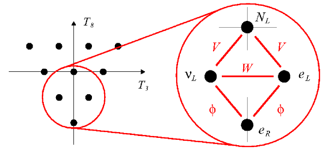
Figure 10: The figure shows the bosonic fields mediating interactions between those states of the $\mathbf{10}$ that localise to the electroweak brane (leptons).

If we further assume that $\phi^{i}$ develops a nonzero v.e.v. $|\phi|=\phi_{0}$, then $\phi^{i}$ takes the role of the Higgs field. If this is the case, two of the chiral states ($R$ and one of the $L$’s) mix together to form a massive electron, while the other two remain massless (neutrinos). The electroweak parameters are then found to be as follows: The electron mass is $m_{e}^{2}=3\phi_{0}^{2}\lambda_{\phi}^{2}/2$, the $W$-boson mass is $M_{W}^{2}=\phi_{0}^{2}\lambda_{H}^{2}/4$, and the electroweak angle is $\sin^{2}\theta_{W}=3\lambda_{G}^{2}/(\lambda_{H}^{2}+3\lambda_{G}^{2})$. Observe that the masses of leptons and $W$ bosons are of the same order. What is more, the quark masses are found to be proportional to $\phi_{0}\lambda_{\phi}$, of the same order as the electron mass. This is because the $\lambda$ couplings are all of the same order. To generate a hierarchy between fermions and gauge bosons, as observed in nature, it is simple a matter of generalising $Y$ to contain other gauge invariant interactions. For example, let us consider a new coupling $Y^{\prime}$ of the form

$$Y^{\prime}=Y-y\,q\,v\,\Theta,$$ (44)

where $q$ is a dimensionless coefficient that could depend on the representation on which $Y^{\prime}$ is acting (observe the similarity of the new term with the old one $-y\,p\,u\,\Phi$, in $Y$). Then, after the scalars have acquired the v.e.v. discussed before, the $Y^{\prime}$ coupling becomes

$$Y^{\prime}(z)=Y(z)-q(yvu)T_{8}.$$ (45)

The second term of this expression resembles the 5-D mass term of Eq. (1). Therefore, the fermion wave functions will split around the branes and an exponential factor, like the one of Eq. (13), will appear suppressing the couplings of Eq. (36). This results in a hierarchy between the mass scales of quarks, leptons and gauge bosons. Observe that in the definition of $Y$ we could also include terms proportional to $\Phi^{2}$ and $\Theta^{2}$ with coefficients depending on the representation. They would provide additional terms contributing to the split of fermions around the brane.

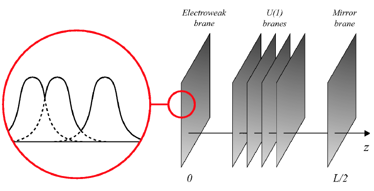
Figure 11: The electroweak brane consists of different fermions with overlapping wave functions.

Very important for this model is that the existence of $V^{i}_{\mu}$ has no conflicts with observations. Fortunately, the mechanism generating the fermion hierarchy is also suppressing the couplings between $V$ and leptons. Additionally, in the case of a nonzero v.e.v. $\phi_{0}$, the four-component vector field $V_{\mu}^{i}$ becomes massive, with $M_{V}^{2}=\phi_{0}^{2}\lambda_{\phi}^{2}\lambda_{Q}^{2}/4\lambda_{4}^{2}$. In fact, the non-observation of $V$-bosons pair-production at LEP [20] is an indication of the constraint

$$M_{V}>104\mathrm{GeV}.$$ (46)

Nevertheless, we should not expect a value $M_{V}$ significantly higher than $M_{Z}$ and $M_{W}$. If this is the case, then we could expect new phenomena associated with extra-dimensions in lepton-collider experiments in the near future.

There are several interesting questions that can be raised about the present model. For example, it would be important to analyse how to include the mixing between different families of leptons and quarks. In the case of leptons, for instance, the new neutrino $N$ could be playing some relevant role in the mixing of neutrinos. Also, it still remains to understand a mechanism to obtain the appropriate potential for the Higgs field $\phi^{i}$.

I would like to acknowledge support from the Swiss National Science Foundation. My gratitude also to the Cambridge Philosophical Society for funding part of my trip to Corfu.

References

References

- [1] Gonzalo A. Palma, Phys. Rev. D 73, 045023 (2006).
- [2] D. B. Fairlie, Phys. Lett. B 82, 97 (1979).
- [3] N.S. Manton, Nucl. Phys. B 158, 141 (1979).
- [4] L.J. Hall, Y. Nomura and D. R. Smith, Nucl. Phys. B 639, 307 (2002).
- [5] G. Burdman and Y. Nomura, Nucl. Phys. B 656, 3 (2003).
- [6] C. Csaki, C. Grojean and H. Murayama, Phys. Rev. D 67, 085012 (2003).
- [7] C. A. Scrucca, M. Serone and L. Silvestrini, Nucl. Phys. B 669, 128 (2003).
- [8] N. Haba and Y. Shimizu, Phys. Rev. D 67, 095001 (2003).
- [9] G. Dvali, S. Randjbar-Daemi and R. Tabbash, Phys. Rev. D 65, 064021 (2002).
- [10] I. Gogoladze, Y. Mimura, S. Nandi, Phys. Lett. B 560, 204 (2003); Phys. Rev. D 69, 075006 (2004).
- [11] K. Agashe, R. Contino and A. Pomarol, Nucl. Phys. B 719, 165 (2005).
- [12] V. A. Rubakov and M. E. Shaposhnikov, Phys. Lett. B 125, 136 (1983).
- [13] N. Arkani-Hamed and M. Schmaltz, Phys. Rev. D 61, 033005 (2000).
- [14] N. Arkani-Hamed, Y. Grossman and M. Schmaltz, Phys. Rev. D 61, 115004 (2000).
- [15] E. A. Mirabelli and M. Schmaltz, Phys. Rev. D 61, 113011 (2000).
- [16] G. Dvali, G. Gabadadze and M. Shifman, Phys. Lett. B 497, 271 (2001).
- [17] G. Dvali, M. Shifman, Phys. Lett. B 396, 64 (1997).
- [18] S. L. Dubovsky, V. A. Rubakov and P. G. Tinyakov, J. High Energy Phys. 08 (2000) 041.
- [19] G. Dvali, G. Gabadadze, M. Porrati, Phys. Lett. B 485, 208 (2000).
- [20] G. Abbiendi, et al. (The OPAL Collaboration), Eur. Phys. J. C 26, 321 (2003).