Topology Change From Quantum Instability of Gauge Theory on Fuzzy ${\rm CP}^{2}$

Abstract

Many gauge theory models on fuzzy complex projective spaces will contain a strong instability in the quantum field theory leading to topology change. This can be thought of as due to the interaction between spacetime via its noncommutativity and the fields (matrices) and it is related to the perturbative UV-IR mixing. We work out in detail the example of fuzzy ${\bf CP}^{2}$ and discuss at the level of the phase diagram the quantum transitions between the $3$ spaces ( spacetimes) ${\bf CP}^{2}$, ${\bf S}^{2}$ and the $0-$dimensional space consisting of a single point $\{0\}$.

The approach of fuzzy physics [1, 2] $1)$ to quantum geometry and $2)$ to non-perturbative field theory insists on the use of finite dimensional matrix algebras with suitable Laplacians ( metrics ) to describe the geometry [3]. Fields will be described by the same matrix algebras or more precisely by the corresponding projective modules [4] and the action functionals will be given by finite dimensional matrix models similar to the IKKT models [5, 6].

As it turns out a topology change can occur naturally if we try to unify spactime and fields using this language of finite dimensional matrices. This is precisely the picture which emerges from the perturbative and non-perturbative studies of noncommutative gauge theory on the fuzzy sphere [7, 8]. Indeed we found in the one-loop calculation [9] as well as in numerical simulations [10, 11] and the large $N$ analysis [12] that the noncommutative gauge model on the fuzzy sphere written in [13] ( which is obtained in the zero-slope limit of string theory ) and its generalizations undergo first order phase transitions from the ”fuzzy sphere” phase to a ”matrix” phase where the fuzzy sphere vacuum collapses under quantum fluctuation. The matrix phase is the space consisting of a single point. This topology change from the two dimensional sphere to a single point and vice versa is intrinsically a quantum mechanical process and it is related to the perturbative UV-IR mixing phenomena. This result was extended to the case of fuzzy ${\bf S}^{2}\times{\bf S}^{2}$ in [14].

In this article we will go one step further and generalize this result to higher fuzzy complex projective spaces. In particular we will work out the case of fuzzy ${\bf CP}^{2}$ in detail. We find the possibility of first order phase transitions between ${\bf CP}^{2}$ and ${\bf S}^{2}$, between ${\bf CP}^{2}$ and a matrix phase and between ${\bf S}^{2}$ and a matrix phase. This richer structure of topology changes is due to the fact that $SU(3)$ contains also $SU(2)$ as a subgroup besides the trivial abelian subgroups $U(1)$. As we will explain generalization of our calculation to higher fuzzy complex projective spaces is obvious and straightforward.

For other approaches to topology change using finite dimensional matrix algebra and fuzzy physics see [15, 16].

This article is organized as follows.

1 Fuzzy ${\bf CP}^{2}$

In this section we will follow [17, 18, 19]. Let $T_{a}$, $a=1,...,8$, be the generators of $SU(3)$ in the symmetric irreducible representation $(n,0)$ of dimension $N=\frac{1}{2}(n+1)(n+2)$. They satisfy

$$[T_{a},T_{b}]=if_{abc}T_{c}\leavevmode\nobreak\$$ (1.1)

and

$$T_{a}^{2}=\frac{1}{3}n(n+3)\equiv|n|^{2}\leavevmode\nobreak\ ,\leavevmode\nobreak\ d_{abc}T_{a}T_{b}=\frac{2n+3}{6}T_{c}.$$ (1.2)

Let $t_{a}=\frac{{\lambda}_{a}}{2}$ ( where ${\lambda}_{a}$ are the usual Gell-Mann matrices ) be the generators of $SU(3)$ in the fundamental representation $(1,0)$ of dimension $N=3$. They also satisfy

$$2t_{a}t_{b}=\frac{1}{3}{\delta}_{ab}+(d_{abc}+if_{abc})t_{c}$$

$$tr_{3}t_{a}t_{b}=\frac{1}{2}{\delta}_{ab}\leavevmode\nobreak\ ,\leavevmode\nobreak\ tr_{3}t_{a}t_{b}t_{c}=\frac{1}{4}(d_{abc}+if_{abc}).$$ (1.3)

The $N-$dimensonal generator $T_{a}$ can be obtained by taking the symmetric product of $n$ copies of the fundamental $3-$dimensional generator $t_{a}$, viz

$$T_{a}=(t_{a}{\otimes}{\bf 1}{\otimes}...{\otimes}{\bf 1}+{\bf 1}{\otimes}t_{a}{\otimes}...{\otimes}{\bf 1}+...+{\bf 1}{\otimes}{\bf 1}{\otimes}...{\otimes}t_{a})_{\rm symmetric}.$$ (1.4)

In the continuum ${\bf CP}^{2}$ is the space of all unit vectors $|\psi>$ in ${\bf C}^{3}$ modulo the phase. Thus $e^{i\theta}|\psi>$, for all $\theta{\in}[0,2\pi[$, define the same point on ${\bf CP}^{2}$. It is obvious that all these vectors $e^{i\theta}|\psi>$ correspond to the same projector $P=|\psi><\psi|$. Hence ${\bf CP}^{2}$ is the space of all projection operators of rank one on ${\bf C}^{3}$. Let ${\bf H}_{N}$ and ${\bf H}_{3}$ be the Hilbert spaces of the $SU(3)$ representations $(n,0)$ and $(1,0)$ respectively. We will define fuzzy ${\bf CP}^{2}$ through the canonical $SU(3)$ coherent states as follows. Let $\vec{n}$ be a vector in ${\bf R}^{8}$, then we define the projector

$$P_{3}=\frac{1}{3}{\bf 1}+n_{a}t_{a}$$ (1.5)

The requirement $P_{3}^{2}=P_{3}$ leads to the condition that $\vec{n}$ is a point on ${\bf CP}^{2}$ satisfying the equations

$$[n_{a},n_{b}]=0\leavevmode\nobreak\ ,\leavevmode\nobreak\ n_{a}^{2}=\frac{4}{3}\leavevmode\nobreak\ ,\leavevmode\nobreak\ d_{abc}n_{a}n_{b}=\frac{2}{3}n_{c}.$$ (1.6)

We can write

$$P_{3}=|\vec{n},3><3,\vec{n}|.$$ (1.7)

We think of $|\vec{n},3>$ as the coherent state in ${\bf H}_{3}$ ( level $3\times 3$ matrices ) which is localized at the point $\vec{n}$ of ${\bf CP}^{2}$. Therefore the coherent state $|\vec{n},N>$ in ${\bf H}_{N}$ ( level $N\times N$ matrices ) which is localized around the point $\vec{n}$ of ${\bf CP}^{2}$ is defined by the projector

$$P_{N}=|\vec{n},N><N,\vec{n}|=(P_{3}{\otimes}P_{3}{\otimes}...{\otimes}P_{3})_{\rm symmetric}.$$ (1.8)

We compute that

$$tr_{3}t_{a}P_{3}=<\vec{n},3|t_{a}|\vec{n},3>=\frac{1}{2}n_{a}\leavevmode\nobreak\ ,\leavevmode\nobreak\ tr_{N}T_{a}P_{N}=<\vec{n},N|T_{a}|\vec{n},N>=\frac{n}{2}n_{a}.$$ (1.9)

Hence it is natural to identify fuzzy ${\bf CP}^{2}$ at level $N=\frac{1}{2}(n+1)(n+2)$ ( or ${\bf CP}^{2}_{n}$ ) by the coordinates operators

$$x_{a}=\frac{2}{n}T_{a}.$$ (1.10)

They satisfy

$$[x_{a},x_{b}]=\frac{2i}{n}f_{abc}x_{c}\leavevmode\nobreak\ ,\leavevmode\nobreak\ x_{a}^{2}=\frac{4}{3}(1+\frac{3}{n})\leavevmode\nobreak\ ,\leavevmode\nobreak\ d_{abc}x_{a}x_{b}=\frac{2}{3}(1+\frac{3}{2n})x_{c}.$$ (1.11)

Therefore in the large $N$ limit we can see that the algebra of $x_{a}$ reduces to the continuum algebra of $n_{a}$. Hence $x_{a}{\longrightarrow}n_{a}$ in the continuum limit $N{\longrightarrow}{\infty}$.

The algebra of  functions on fuzzy ${\bf CP}^{2}_{n}$ is identified with the algebra of $N{\times}N$ matrices $Mat_{N}$ generated by all polynomials in the coordinates operators $x_{a}$. Recall that $N=\frac{1}{2}(n+1)(n+2)$. The left action of $SU(3)$ on this algebra is generated by $(n,0)$ whereas the right action is generated by $(0,n)$. Thus the algebra $Mat_{N}$ decomposes under the action of $SU(3)$ as

$$(n,0){\otimes}(0,n)={\otimes}_{p=0}^{n}(p,p).$$ (1.12)

A general function on fuzzy ${\bf CP}^{2}_{n}$ is therefore written as

$$F=\sum_{p=0}^{n}F_{I^{2},I_{3},Y}^{(p)}T_{I^{2},I_{3},Y}^{(p,p)}$$ (1.13)

$T_{I^{2},I_{3},Y}^{(p,p)}$ are $SU(3)$ polarization tensors in the irreducible representation $(p,p)$. $I^{2},I_{3}$ and $Y$ are the square of the isospin, the third component of the isospin and the hypercharge quantum numbers which characterize $SU(3)$ representations.

The derivations on fuzzy ${\bf CP}^{2}_{n}$ are defined by the commutators $[T_{a},..]$. The Laplacian is then obviously given by ${\Delta}_{N}=[T_{a},[T_{a},...]]$. Fuzzy ${\bf CP}^{2}_{n}$ is completely determined by the spectral triple ${\bf CP}^{2}_{n}=(Mat_{N},{\Delta}_{N},{\bf H}_{N})$. Now we can compute

$$tr_{N}FP_{N}=<\vec{n},N|F|\vec{n},N>=F_{N}(\vec{n})=\sum_{p=0}^{n}F_{I^{2},I_{3},Y}^{(p)}Y_{I^{2},I_{3},Y}^{(p,p)}(\vec{n})$$ (1.14)

$Y_{I^{2},I_{3},Y}^{(p,p)}(\vec{n})$ are $SU(3)$ polarization tensors defined by

$$Y_{I^{2},I_{3},Y}^{(p,p)}(\vec{n})=<\vec{n},N|T_{I^{2},I_{3},Y}^{(p,p)}|\vec{n},N>.$$ (1.15)

Furthermore we can compute

$$tr_{N}[T_{a},F]P_{N}=<\vec{n},N|[T_{a},F]|\vec{n},N>=({\cal L}_{a}F_{N})(\vec{n})\leavevmode\nobreak\ ,\leavevmode\nobreak\ {\cal L}_{a}=-if_{abc}n_{b}{\partial}_{c}.$$ (1.16)

And

$$tr_{N}FGP_{N}=<\vec{n},N|FG|\vec{n},N>=F_{N}*G_{N}(\vec{n}).$$ (1.17)

The star product on fuzzy ${\bf CP}^{2}_{n}$ is found to be given by [19]

$$F_{N}*G_{N}(\vec{n})=\sum_{p=0}^{n}\frac{(n-p)!}{p!n!}K_{a_{1}b_{1}}...K_{a_{p}b_{p}}{\partial}_{a_{1}}...{\partial}_{a_{p}}F_{N}(\vec{n}){\partial}_{b_{1}}...{\partial}_{b_{p}}G_{N}(\vec{n})\leavevmode\nobreak\$$

$$\leavevmode\nobreak\ K_{ab}=\frac{2}{3}{\delta}_{ab}-n_{a}n_{b}+(d_{abc}+if_{abc})n_{c}.$$ (1.18)

2 Fuzzy gauge fields on ${\bf CP}^{2}_{n}$

We will introduce fuzzy gauge fields $A_{a}$, $a=1,...,8$, through the covariant derivatives $D_{a}$, $a=1,...,8$, as follows

$$D_{a}=T_{a}+A_{a}.$$ (2.1)

$D_{a}$ are $N{\times}N$ matrices which transform under the action of $U(N)$ as follows $D_{a}{\longrightarrow}UD_{a}U^{+}$ where $U{\in}U(N)$. Hence $A_{a}$ are $N{\times}N$ matrices which transform as $A_{a}{\longrightarrow}UA_{a}U^{+}+U[T_{a},U^{+}]$. In order that the field $\vec{A}$ be a $U(1)$ gauge field on fuzzy ${\bf CP}^{2}_{n}$ it must satisfies some additional constraints so that only four of its components are non-zero. These are the tangent components to ${\bf CP}^{2}_{n}$. The other four components of $\vec{A}$ are normal to ${\bf CP}^{2}_{n}$ and in general they will be projected out from the model.

Let us go back to the continuum ${\bf CP}^{2}$ and let us consider a gauge field $A_{a}$, $a=1,...,8$, which is strictly tangent to ${\bf CP}^{2}$ . By construction this gauge field must satisfy

$$A_{a}=P_{ab}^{T}A_{b}\leavevmode\nobreak\ ,\leavevmode\nobreak\ P^{T}=(n_{a}Adt_{a})^{2}.$$ (2.2)

$P^{T}$ is the projector which defines the tangent bundle over ${\bf CP}^{2}$. The normal bundle over ${\bf CP}^{2}$ will be defined by the projector $P^{N}=1-P^{T}$. Explicitly these are given by

$$P^{T}_{ab}=n_{c}n_{d}(Adt_{c})_{ae}(Adt_{d})_{eb}=n_{c}n_{d}f_{cae}f_{dbe}\leavevmode\nobreak\ ,\leavevmode\nobreak\ P^{N}_{ab}={\delta}_{ab}-n_{c}n_{d}f_{cae}f_{dbe}.$$ (2.3)

In above we have used the fact that the generators in the adjoint representation $(1,1)$ satisfy $(Adt_{a})_{bc}=-if_{abc}$. Remark that we have the identities $n_{a}P^{T}_{ab}=n_{b}P^{T}_{ab}=0$. Hence the condition (2.2) takes the natural form

$$n_{a}A_{a}=0.$$ (2.4)

This is one condition which allows us to reduce the number of independent components of $A_{a}$ by one. We know that there must be three more independent constraints which the tangent field $A_{a}$ must satisfy since it has only $4$ independent components. To find them we start from the identity [20]

$$d_{abk}d_{cdk}=\frac{1}{3}\bigg{[}{\delta}_{ac}{\delta}_{bd}+{\delta}_{bc}{\delta}_{ad}-{\delta}_{ab}{\delta}_{cd}+f_{cak}f_{dbk}+f_{dak}f_{cbk}\bigg{]}.$$ (2.5)

Thus

$$n_{c}n_{d}d_{abk}d_{cdk}=\frac{2}{3}\bigg{[}{n}_{a}{n}_{b}-\frac{2}{3}{\delta}_{ab}+n_{c}n_{d}f_{cak}f_{dbk}\bigg{]}.$$ (2.6)

By using the fact that $d_{cdk}n_{c}n_{d}=\frac{2}{3}n_{k}$ we obtain

$$d_{abk}n_{k}={n}_{a}{n}_{b}-\frac{2}{3}{\delta}_{ab}+n_{c}n_{d}f_{cak}f_{dbk}.$$ (2.7)

Hence it is a straightforward calculation to find that the gauge field $A_{a}$ must also satisfy the conditions

$$d_{abk}n_{k}A_{b}=\frac{1}{3}A_{a}.$$ (2.8)

In the case of ${\bf S}^{2}$ the projector $P^{T}$ takes the simpler form $P^{T}_{ab}={\delta}_{ab}-n_{a}n_{b}$ and hence $P^{N}_{ab}=n_{a}n_{b}$. From equation (2.7) we have on ${\bf CP}^{2}$

$$P_{ab}^{T}=d_{abc}n_{c}-n_{a}n_{b}+\frac{2}{3}{\delta}_{ab}\leavevmode\nobreak\ ,\leavevmode\nobreak\ P_{ab}^{N}=-d_{abc}n_{c}+n_{a}n_{b}+\frac{1}{3}{\delta}_{ab}.$$ (2.9)

If we choose to sit on the “north pole” of ${\bf CP}^{2}$, i.e $\vec{n}=(0,0,0,0,0,0,0,-\frac{2}{\sqrt{3}})$ then we can find that $P^{T}=diag(0,0,0,1,1,1,1,0)$ and as a consequence $P^{N}=(1,1,1,0,0,0,0,1)$ . So $Adt_{a}$, $a=1,2,3,8$ correspond to the normal directions while $Adt_{a}$, $a=4,5,6,7$ correspond to the tangent directions.

Indeed by substituting $\vec{n}=(0,0,0,0,0,0,0,-\frac{2}{\sqrt{3}})$ in equation (2.8) and using $d_{8ij}=\frac{1}{\sqrt{3}}{\delta}_{ij}$ where $i,j=1,2,3$ and $d_{8\alpha\alpha}=-\frac{1}{2\sqrt{3}}$ where $\alpha=4,5,6,7$ and $d_{888}=-\frac{1}{\sqrt{3}}$ we get $A_{1}=A_{2}=A_{3}=A_{8}=0$ which is what we want. In fact (2.8) already contains (2.4). In other words it contains exactly the correct number of equations needed to project out the gauge field $A_{a}$ onto the tangent bundle of ${\bf CP}^{2}$.

Let us finally say that given any continuum gauge field $A_{a}$ which does not satisfy the constraints (2.4) and (2.8) we can always make it tangent by applying the projector $P^{T}$. Thus we will have the tangent gauge field

$$A_{a}^{T}=P_{ab}^{T}A_{b}=d_{abc}n_{c}A_{b}-n_{a}(n_{b}A_{b})+\frac{2}{3}A_{a}.$$ (2.10)

Similarly the fuzzy gauge field must satisfy some conditions which should reduce to (2.4) and (2.8). As it turns out constructing a tangent fuzzy gauge field using an expression like (2.2) is a highly non-trivial task due to $1)$ gauge covariance problems and $2)$ operator ordering problems. However implementing (2.4) and (2.8) in the fuzzy setting is quite easy since we will only need to return to the covariant derivatives $D_{a}$ and require them to satisfy the $SU(3)$ identities (1.2), viz

$$D_{a}^{2}=\frac{1}{3}n(n+3)$$

$$d_{abc}D_{a}D_{b}=\frac{2n+3}{6}D_{c}.$$ (2.11)

So $D_{a}$ are almost the $SU(3)$ generators except that they fail to satisfy the fundamental commutation relations of $SU(3)$ given by equation (1.1). This failure is precisely measured by the curvature of the gauge field $A_{a}$, namely

$$F_{ab} = i[D_{a},D_{b}]+f_{abc}D_{c}$$ (2.12)

$$= i[T_{a},A_{b}]-i[T_{b},A_{a}]+f_{abc}A_{c}+i[A_{a},A_{b}].$$

The continuum limit of this object is clearly given by the usual curvature on ${\bf CP}^{2}$, viz $F_{ab}=i{\cal L}_{a}A_{b}-i{\cal L}_{b}A_{a}+f_{abc}A_{c}+i[A_{a},A_{b}]$. To check that this fuzzy gauge field $A_{a}$ has the correct degrees of freedom we need to check that the identities (2.11) reduce to (2.4) and (2.8) in the continuum limit $n{\longrightarrow}\infty$. This fact is quite straightforward to verify and we leave it as an exercise.

Next we need to write down actions on fuzzy ${\bf CP}^{2}_{n}$. The first piece is the usual Yang-Mills action

$$S_{\rm YM}=\frac{1}{4g^{2}}Tr_{N}F_{ab}^{2}.$$ (2.13)

By construction it has the correct continuum limit. $Tr_{N}$ is the normalized trace $Tr_{N}{\bf 1}=1$.

The second piece in the action is a potential term which has to implement the constraints (2.11) in some limit. Indeed we will not impose these constraints rigidly on the path integral but we will include their effects by adding to the action a very special potential term. In other words we will not assume that $D_{a}$ satisfy (2.11). To the end of writing this potential term we will introduce the four normal scalar fields on fuzzy ${\bf CP}^{2}_{n}$ by the equations ( see equations (2.11) )

$${\Phi}=\frac{1}{n}(D_{a}^{2}-\frac{1}{3}n(n+3))=\frac{1}{2}x_{a}A_{a}+\frac{1}{2}A_{a}x_{a}+\frac{1}{n}A_{a}^{2}{\longrightarrow}n_{a}A_{a}$$ (2.14)

and

$${\Phi}_{c}=\frac{1}{n}(d_{abc}D_{a}D_{b}-\frac{2n+3}{6}D_{c}) = \frac{1}{2}d_{abc}x_{a}A_{b}+\frac{1}{2}d_{abc}A_{a}x_{b}-\frac{2n+3}{6n}A_{c}+\frac{1}{n}d_{abc}A_{a}A_{b}$$ (2.15)

$${\longrightarrow} d_{abc}n_{a}A_{b}-\frac{1}{3}A_{c}.$$

We add to the Yang-Mills action the potential term

$$V_{0}=\beta Tr_{N}{\Phi}^{2}+M^{2}Tr_{N}{\Phi}_{a}^{2}.$$ (2.16)

In the limit where the parameters $\beta$ and $M^{2}$ are taken to be very large positive numbers we can see that only configurations $A_{a}$ ( or equivalently $D_{a}$ ) such that $\Phi=0$ and ${\Phi}_{c}=0$ dominate the path integral which is precisely what we want. This is the region of the phase space of most interest. This is the classical prediction.

However in the quantum theory we will find that the parameter $\beta$ must be related to $M^{2}$ in some specific way in order to kill exactly the normal components of $A_{a}$. This result ( which we will show shortly in the one-loop quantum fuzzy theory ) is the quantum analogue of the classical continuum statement that equation (2.8) contains already (2.4).

3 The classical and one-loop quantum actions on ${\bf CP}^{2}_{n}$

The total action is then given by

$$S_{1} = \frac{1}{2g^{2}}Tr_{N}F_{ab}^{2}+\beta Tr_{N}{\Phi}^{2}+M^{2}Tr_{N}{\Phi}_{c}^{2}$$ (3.1)

$$= \frac{1}{g^{2}}Tr_{N}\bigg{[}-\frac{1}{4}[D_{a},D_{b}]^{2}+if_{abc}D_{a}D_{b}D_{c}\bigg{]}+\frac{3n}{4g^{2}}Tr_{N}\Phi+\beta Tr_{N}{\Phi}^{2}+M^{2}Tr_{N}{\Phi}_{c}^{2}.$$

This is essentially the same action considered in [20]. However this action is different from the action considered in [10] which is of the form

$$S_{0} = \frac{1}{g^{2}}Tr_{N}\bigg{[}-\frac{1}{4}[D_{a},D_{b}]^{2}+\frac{2i}{3}f_{abc}D_{a}D_{b}D_{c}\bigg{]}.$$ (3.2)

The first difference is between the cubic terms which come with different coefficients. The second more crucial difference is the presence of the potential term in our case. The linear term in $\Phi$ is actually a part of the Yang-Mills action.

The equations of motion derived from the action $S_{0}$ are

$$[D_{a},F_{ab}]=0.$$ (3.3)

These are solved by the fuzzy ${\bf CP}^{2}_{n}$ configurations

$$D_{a}=T_{a}$$ (3.4)

and also by the diagonal matrices

$$D_{a}={\rm diag}(d_{a}^{1},d_{a}^{2},...,d_{a}^{N}).$$ (3.5)

We think of these diagonal matrices ( including the zero matrix ) as describing a single point in accordance with the IKKT model [5].

More interestingly is the fact that these equations of motion are also solved by the fuzzy ${\bf S}^{2}_{N}$ configurations

$$D_{i}=L_{i}\leavevmode\nobreak\ ,\leavevmode\nobreak\ i=1,2,3\leavevmode\nobreak\ {\rm and}\leavevmode\nobreak\ D_{\alpha}=0\leavevmode\nobreak\ {\alpha}=4,5,6,7,8.$$ (3.6)

Indeed in this case $[D_{a},F_{ab}]=[D_{i},F_{ib}]$. For $b=j$ this is equal to $0$ because $f_{ijk}={\epsilon}_{ijk}$ whereas for $b=\alpha$ this is equal to zero because $f_{ij\alpha}=0$. In above $L_{i}$ are the generators of $SU(2)$ in the irreducible representation $\frac{N-1}{2}$.

The equations of motion derived from the action $S_{1}$ are on the other hand given by

$$\frac{i}{g^{2}}[D_{b},F_{ab}]+\frac{1}{2g^{2}}f_{abc}F_{bc}+2\beta\{\Phi,D_{a}\}+M^{2}\bigg{(}2d_{abc}\{{\Phi}_{c},D_{b}\}-\frac{2n+3}{3}{\Phi}_{a}\bigg{)}=0.$$ (3.7)

Now the only solutions of these equations of motion are the ${\bf CP}^{2}_{n}$ configurations (3.4). Thus the potential term has eliminated the diagonal matrices (3.5) as possible solutions. In fact this classical observation will not hold in the quantum theory for all values of the parameter $M^{2}$ since there will always be a region in the phase space of the theory where the vacuum solution is not $D_{a}=T_{a}$ but $D_{a}=0$. However when we take $M^{2}$ to be very large positive number then we can see that $D_{a}=T_{a}$ becomes quantum mechanically more stable. Hence by neglecting the potential term we can not at all speak of the space ${\bf CP}^{2}_{n}$ since it will collapse rather quickly under quantum fluctuations to a single point.

The potential term has also eliminated the fuzzy ${\bf S}^{2}_{N}$ configurations (3.6) as possible solutions. In fact even if we set $M=\beta=0$ in the above equations of motion the fuzzy ${\bf S}^{2}_{N}$ configurations (3.6) are not solutions.

The other major difference between $S_{1}$ and $S_{0}$ is that if we expand around the fuzzy ${\bf CP}^{2}_{n}$ solution $D_{a}=T_{a}$ by writing $D_{a}=T_{a}+A_{a}$ and then substitute back in $S_{1}$ and $S_{0}$ we find that $S_{0}$ does not yield in the continuum limit the usual pure gauge theory on ${\bf CP}^{2}$. It contains an extra piece which resembles the Chern-Simons action ( although it is strictly real ). We skip here the corresponding elementary proof ( see the appendix ). $S_{1}$ will yield on the other hand the desired pure gauge theory on ${\bf CP}^{2}_{n}$ in the limit $M^{2}{\longrightarrow}\infty$ and hence it has the correct continuum limit. If we do not take the limit $M^{2}{\longrightarrow}\infty$ then $S_{1}$ will describe a gauge theory coupled to $4$ adjoint scalar fields which are the normal components of $A_{a}$.

The only motivation for $S_{0}$-as far as we can see- is its similarity to the fuzzy ${\bf S}^{2}$ action which looks precisely like $S_{0}$ with the replacement $f_{abc}{\longrightarrow}{\epsilon}_{abc}$. This fuzzy sphere action was obtained in string theory in the limit ${\alpha}^{{}^{\prime}}{\longrightarrow}0$ when we have open strings moving in a curved background with an ${\bf S}^{3}$ metric in the presence of a Neveu-Schwarz B-field. However it is found that perturbation theory with $S_{0}$ is simpler than perturbation theory with $S_{1}$. More importantly it is found that $S_{0}$ allows for some new topology change which does not occur with $S_{1}$. In particular the transitions ${\bf CP}^{2}_{n}{\longrightarrow}{\bf S}^{2}_{N}$ and ${\bf S}^{2}_{N}{\longrightarrow}{\bf CP}^{2}_{n}$ are possible in the quantum theory of $S_{0}$.

Using the background field method we find that the one-loop effective action in the gauge ${\xi}^{-1}=1+\frac{2g^{2}{\beta}_{i}}{n^{2}}$ is given by ( see the appendix )

$${\Gamma}_{i}[D] = {S}_{i}[D]+\frac{1}{2}Tr_{8}TR\log{\Omega}^{i}_{ab}-TR\log{\cal D}_{a}^{2}.$$ (3.8)

Where

$${S}_{i}[D] = \frac{1}{g^{2}}Tr_{N}\bigg{(}-\frac{1}{4}[D_{a},D_{b}]^{2}+i{\alpha}_{i}f_{abc}D_{a}D_{b}D_{c}\bigg{)}+{\rho}_{i}Tr_{N}\Phi+{\beta}_{i}Tr_{N}{\Phi}^{2}+M_{i}^{2}Tr_{N}{\Phi}_{c}^{2}.$$

And

$${\Omega}^{i}_{ab} = {\cal D}_{c}^{2}{\delta}_{ab}-2i{\cal F}_{ab}+2i(1-\frac{3{\alpha}_{i}}{2})f_{abc}{\cal D}_{c}+\frac{2g^{2}{\rho}_{i}}{n}{\delta}_{ab}+\frac{2g^{2}{\beta}_{i}}{n^{2}}\big{(}4D_{a}D_{b}+2n{\delta}_{ab}\Phi\big{)}+\frac{2g^{2}M_{i}^{2}}{n^{2}}\bigg{(}$$

$$- d_{aa^{{}^{\prime}}c}d_{bb^{{}^{\prime}}c}{\cal D}_{a^{{}^{\prime}}}{\cal D}_{b^{{}^{\prime}}}+4d_{aa^{{}^{\prime}}c}d_{bb^{{}^{\prime}}c}D_{a^{{}^{\prime}}}D_{b^{{}^{\prime}}}-2(\frac{2n+3}{3})d_{abc}D_{c}+2nd_{abc}{\Phi}_{c}+(\frac{2n+3}{6})^{2}{\delta}_{ab}\bigg{)}.$$

The trace $TR$ corresponds to the left and right actions of operators on matrices whereas $Tr_{8}$ is the trace associated with $8-$dimensional rotations. Given a matrix $O$ the operator ${\cal O}$ is given by ${\cal O}(..)=[O,..]$, for example ${\cal D}_{a}(Q_{a})=[D_{a},Q_{a}]$. For $S_{0}$ we have ${\alpha}_{0}=\frac{2}{3}$, ${\rho}_{0}={\beta}_{0}=M_{0}=0$ while for $S_{1}$ we have ${\alpha}_{1}=1$, ${\rho}_{1}=\frac{3n}{4g^{2}}$, ${\beta}_{1}=\beta$ and $M_{1}=M$.

4 Fuzzy ${\bf CP}^{2}$ phase and a stable fuzzy sphere phase

Fuzzy ${\bf CP}^{2}$ phase

Let us first neglect the potential term in $S_{i}$, i.e we will set ${\beta}_{i}=M_{i}=0$ or equivalently $V_{0}=0$ in $S_{1}$. The effective potential is given by the formula (3.8), viz

$${\Gamma}_{i}[D] = S_{i}[D]+\frac{1}{2}Tr_{8}TR\log{\Omega}^{i}_{ab}-TR\log{\cal D}_{a}^{2}$$ (4.1)

where the background field is chosen such that

$$D_{a}=\phi T_{a}.$$ (4.2)

The reason is simply because we want to study the stability of the fuzzy ${\bf CP}^{2}_{n}$ vacuum $D_{a}=T_{a}$ against quantum fluctuations. Hence $\phi$ is an order parameter which measures in a well defined obvious sense the radius of ${\bf CP}^{2}_{n}$. Let us compute the classical potential in this configuration. we have

$$S_{i}[D] = \frac{3|n|^{2}}{g^{2}}\bigg{[}\frac{1}{4}{\phi}^{4}-\frac{{\alpha}_{i}}{2}{\phi}^{3}+\frac{g^{2}{\rho}_{i}}{3n}({\phi}^{2}-1)\bigg{]}.$$ (4.3)

The main quantum correction is equal to the trace of the logarithm of the Laplacian ${\Omega}^{i}$ which is given by the simple formula

$${\Omega}^{i}_{ab} = \bigg{(}{\phi}^{2}{\cal L}_{c}^{2}+\frac{2g^{2}{\rho}_{i}}{n}\bigg{)}{\delta}_{ab}+2i\phi(\phi-\frac{3{\alpha}_{i}}{2})f_{abc}{\cal L}_{c}$$ (4.4)

where ${\cal L}_{a}(..)=[T_{a},..]$. There are two cases to consider. For both $S_{0}$ and $S_{1}$ we obtain the quantum correction ( see the appendix )

$${\Delta}{\Gamma}_{i}[D] = \frac{1}{2}Tr_{8}TR\log({\phi}^{2}{\cal L}_{a}^{2}{\bf 1}_{8})-TR\log({\phi}^{2}{\cal L}_{a}^{2})$$ (4.5)

$$= +6N^{2}\log{\phi}+{\rm constant}.$$

Case $1$

For $S_{0}$ we have ${\alpha}_{0}=\frac{2}{3}$ and ${\rho}_{0}=0$. Thus the quantum effective potential is

$$V_{\rm eff}=\frac{{\Gamma}_{0}[D]}{6N^{2}} = \frac{2}{3n^{2}g^{2}}\bigg{[}\frac{1}{4}{\phi}^{4}-\frac{1}{3}{\phi}^{3}\bigg{]}+\log{\phi}+{\rm constant}.$$ (4.6)

The quantum minimum of the model is given by the value of $\phi$ which solves the equation $V_{\rm eff}^{{}^{\prime}}=0$. It is not difficult to convince ourselves that this equation of motion will admit a solution only up to an upper critical value $g_{*}$ of the gauge coupling constant $g$ beyond which the configuration $D_{a}=\phi T_{a}$ collapses. At this value $g_{*}$ the potential $V_{\rm eff}$ becomes unbounded from below. The conditions which will yield the critical value $g_{*}$ are therefore

$$V_{\rm eff}^{{}^{\prime}}=\frac{2}{3n^{2}g^{2}}\bigg{[}{\phi}^{3}-{\phi}^{2}\bigg{]}+\frac{1}{\phi}=0\leavevmode\nobreak\ ,\leavevmode\nobreak\ V_{\rm eff}^{{}^{\prime\prime}}=\frac{2}{3n^{2}g^{2}}\bigg{[}3{\phi}^{2}-2{\phi}\bigg{]}-\frac{1}{{\phi}^{2}}=0.$$ (4.7)

We find immediately

$${\phi}_{*}=\frac{3}{4}\leavevmode\nobreak\ ,\leavevmode\nobreak\ n^{2}g_{*}^{2}=\frac{2}{9}(\frac{3}{4})^{4}=0.0703.$$ (4.8)

Above the value $g_{*}$ we do not have a fuzzy ${\bf CP}^{2}_{n}$, in other words the space ${\bf CP}^{2}_{n}$ evaporates at this point. This critical point separates two distinct phases of the model, in the region above $g_{*}$ we have a “matrix phase” while in the region below $g_{*}$ we have a “fuzzy ${\bf CP}^{2}_{n}$” phase in which the model admits the interpretation of being a $U(1)$ gauge theory on ${\bf CP}^{2}$.

By going from small values of $g$ ( $g{\leq}g_{*}$ corresponding to the “fuzzy ${\bf CP}_{n}^{2}$ phase” ) towards large values of $g$ we get through the value $g_{*}$ where the space ${\bf CP}^{2}_{n}$ decays. Looking at this process the other way around we can see that starting from large values of $g$ ( $g{>}g_{*}$ corresponding to the “matrix phase” ) and going through $g_{*}$ we generate the space ${\bf CP}^{2}_{n}$ dynamically. It seems therefore that we have generated quantum mechanically the spectral triple which defines the space ${\bf CP}^{2}_{n}$.

Furthermore we note that in the “matrix phase” we have a $U(N)$ gauge theory reduced to a point where $N$ is the size of the matrices since the minimum there is given by diagonal matrices. The important point is that in this phase the gauge group is certainly not $U(1)$. Let us recall that in the “fuzzy ${\bf CP}^{2}_{n}$ phase” we had a $U(1)$ gauge theory. Hence across the transition line between the “fuzzy ${\bf CP}^{2}_{n}$ phase” and the “matrix phase” the structure of the gauge group also changes. Thus we obtain in this model in correlation with the topology change across the critical line a novel spontaneous symmetry breaking mechanism.

For the purpose of comparing with the numerical results of  [10] we define the coupling constant $\bar{\alpha}$ such that $\bar{\alpha}^{4}N=\frac{1}{g^{2}}$. Then the critical value (4.8) is seen to occur at

$$\bar{\alpha}_{*}=2.309.$$ (4.9)

This is precisely the result of the Monte Carlo simulation reported in equation $(3.2)$ of [10].

Case $2$

For $S_{1}$ we have ${\alpha}_{1}=1$ and ${\rho}_{1}=\frac{3n}{4g^{2}}$ and hence the effective potential is given by

$$V_{\rm eff}=\frac{{\Gamma}_{1}[D]}{6N^{2}} = \frac{2}{3n^{2}g^{2}}\bigg{[}\frac{1}{4}{\phi}^{4}-\frac{1}{2}{\phi}^{3}+\frac{1}{4}{\phi}^{2}\bigg{]}+\log{\phi}+{\rm constant}.$$ (4.10)

A direct calculation yields the critical values

$${\phi}_{*}=\frac{9+\sqrt{17}}{16}\leavevmode\nobreak\ ,\leavevmode\nobreak\ n^{2}g_{*}^{2}=\frac{{\phi}_{*}^{2}}{4}({\phi}_{*}-\frac{2}{3})=0.02552.$$ (4.11)

This $g_{*}$ is smaller than the $g_{*}$ obtained in (4.8) and hence the fuzzy ${\bf CP}^{2}_{n}$ is more stable in the model $S_{0}$ than it is in the model $S_{1}$ which is largely due to the linear term proportional to $\Phi$ in $S_{1}$. In other words attempting to put true gauge theory on fuzzy ${\bf CP}^{2}_{n}$ causes the space to decay more rapidly. However for $S_{0}$ the true vacuum is the fuzzy sphere ${\bf S}^{2}_{N}$ and not the fuzzy ${\bf CP}^{2}_{n}$ as we will now discuss

A stable fuzzy sphere phase

We know that there is also a fuzzy sphere solution (3.6) for the model $S_{0}$. We consider then the background field

$$D_{i}=\phi T_{i}\leavevmode\nobreak\ ,\leavevmode\nobreak\ i=1,2,3\leavevmode\nobreak\ ,D_{\alpha}=0\leavevmode\nobreak\ ,\leavevmode\nobreak\ \alpha=4,5,6,7,8.$$ (4.12)

We want now to study the stability of this vacuum against quantum fluctuations. The $\phi$ is now an order parameter which measures the radius of the fuzzy sphere ${\bf S}^{2}_{N}$. The classical potential in this configuration is

$$S_{0}[D] = \frac{2c_{2}}{g^{2}}\bigg{[}\frac{1}{4}{\phi}^{4}-\frac{1}{3}{\phi}^{3}\bigg{]}.$$ (4.13)

In above $c_{2}=\frac{N^{2}-1}{4}$ is the Casimir of $SU(2)$ in the irreducible representation $\frac{N-1}{2}$ ( $N=\frac{1}{2}(n+1)(n+2)$ ). It is clear that $2c_{2}>>3|n|^{2}$ and $\frac{|n|^{2}}{c_{2}}<<1$ in the large $n$ limit. Hence the action (4.13) around the classical minimum $\phi=1$ is much smaller than the classical action (4.3). In other words the fuzzy sphere is more stable than the fuzzy ${\bf CP}^{2}_{n}$ in this case.

The quantum corrections are given in this case by

$$\frac{1}{2}Tr_{3}TR\log{\Omega}_{ij}+\frac{1}{2}Tr_{5}TR\log\tilde{\Omega}_{\alpha\beta}-TR\log{\phi}^{2}{\cal L}_{i}^{2}.$$ (4.14)

In above

$${\Omega}_{ij} = \bigg{(}{\phi}^{2}{\cal L}_{k}^{2}+\frac{2g^{2}\rho}{n}\bigg{)}{\delta}_{ij}+2i\phi(\phi-\frac{3\alpha}{2}){\epsilon}_{ijk}{\cal L}_{k}\leavevmode\nobreak\ ,\leavevmode\nobreak\ \tilde{\Omega}_{\alpha\beta}=\bigg{(}{\phi}^{2}{\cal L}_{k}^{2}+\frac{2g^{2}\rho}{n}\bigg{)}{\delta}_{\alpha\beta}-3i\alpha\phi f_{\alpha\beta i}{\cal L}_{i}.$$

Following the same arguments of the previous section ( only now it is $SU(2)$ representation theory which is involved ) we have in the large $n$ limit

$$\frac{1}{2}Tr_{3}TR\log{\Omega}_{ij}-TR\log{\phi}^{2}{\cal L}_{i}^{2}=\frac{1}{2}Tr_{3}TR\log{\phi}^{2}{\delta}_{ij}-TR\log{\phi}^{2}+..=N^{2}\log\phi+...$$ (4.16)

We can also argue that we have

$$\frac{1}{2}Tr_{5}TR\log{\Omega}_{\alpha\beta}+..=5N^{2}\log\phi+...$$ (4.17)

In other words the configurations (4.12) although they are fuzzy sphere configurations they know ( through their quantum interactions ) about the other $SU(3)$ structure present in the model. Classically this $SU(3)$ structure is not detected at all by these configurations in the classical potential (4.13). The effective potential becomes in this case

$$V_{\rm eff}=\frac{{\Gamma}_{0}[D]}{6N^{2}} = \frac{1}{12g^{2}}\bigg{[}\frac{1}{4}{\phi}^{4}-\frac{1}{3}{\phi}^{3}\bigg{]}+\log{\phi}+{\rm constant}.$$ (4.18)

A direct calculation yields the critical value

$${\phi}_{*}=\frac{3}{4}\leavevmode\nobreak\ ,\leavevmode\nobreak\ g_{*}^{2}=\frac{1}{36}(\frac{3}{4})^{4}=0.0087875.$$ (4.19)

In terms of the coupling $\tilde{\alpha}$ define by $\tilde{\alpha}^{4}=\frac{1}{g^{2}}$ the critical value $g_{*}$ reads

$$\tilde{\alpha}_{*}=3.26.$$ (4.20)

This is again what is measured in the Monte Carlo simulation of the model $S_{0}$ as it is reported in equation $(4.2)$ of [10]. Therefore we have a fuzzy sphere phase above $\tilde{\alpha}_{*}$ and a matrix phase below $\tilde{\alpha}_{*}$. The model $S_{0}$ can also be in a fuzzy ${\bf CP}^{2}_{n}$ phase for $n^{2}g_{*}^{2}$ below the second value of (4.8) which for large enough $n$ is much smaller than the value $n^{2}g_{*}^{2}$ with $g_{*}^{2}$ given by the second equation of (4.19). However we have seen in the previous paragraph that this ${\bf CP}_{n}^{2}$ will decay rather quickly to a single point which ( by the discussion of the present section ) can only happen by going first across a fuzzy sphere phase. We have then the transition pattern ${\bf CP}^{2}_{n}{\longrightarrow}{\bf S}^{2}_{N}{\longrightarrow}\{0\}$. In the limit where $\bar{\alpha}^{4}={2}/{n^{2}g^{2}}$ is kept fixed we can see that the above critical value (4.19) is infinitely large which means that the model $S_{0}$ is mostly in the fuzzy sphere phase. The matrix phase shrinks to zero and the fuzzy sphere is completely stable in this limit since the fuzzy ${\bf CP}^{2}_{n}$ phase can occur only at very small values of the coupling constant $n^{2}g^{2}$.

5 The large mass limit and the transition ${\bf CP}^{2}{\longrightarrow}{\bf S}^{2}$

The large mass limit

Now we include the effect of the potential term $V_{0}$. The relevant model is given by the action $S_{1}$. Naturally the calculation becomes more complicated in this case. The classical potential in the configuration $D_{a}=\phi T_{a}$ is

$$\frac{S_{1}[D]}{6N^{2}} = \frac{2}{3n^{2}g^{2}}\bigg{[}\frac{1}{4}{\phi}^{4}-\frac{1}{2}{\phi}^{3}+\frac{1}{4}{\phi}^{2}+\frac{g^{2}\beta}{9}({\phi}^{2}-1)^{2}+\frac{g^{2}M^{2}}{27}({\phi}^{2}-\phi)^{2}\bigg{]}.$$ (5.1)

The most important quantum correction is given by the determinant of

$${\Omega}^{1}_{ab} = \bigg{(}{\phi}^{2}{\cal L}_{c}^{2}+\frac{3}{2}\bigg{)}{\delta}_{ab}-2\phi(\phi-\frac{3}{2})(Adt_{c}{\cal L}_{c})_{ab}+2g^{2}{\beta}{\Delta}_{1}{\Omega}_{ab}+2g^{2}M^{2}{\Delta}_{2}{\Omega}_{ab}.$$ (5.2)

By using the identities (1.2) and (2.5) we find that the extra contributions are given explicitly by the expressions

$${\Delta}_{1}{\Omega}_{ab}=\frac{1}{n^{2}}\bigg{[}4{\phi}^{2}T_{a}T_{b}+2({\phi}^{2}-1)T_{c}^{2}{\delta}_{ab}\bigg{]}.$$ (5.3)

$${\Delta}_{2}{\Omega}_{ab} = \frac{1}{n^{2}}\bigg{[}(\frac{2n+3}{6})^{2}{\delta}_{ab}+({\phi}^{2}-3{\phi})(\frac{2n+3}{3})d_{abc}T_{c}$$ (5.4)

$$+ \frac{4{\phi}^{2}}{3}\bigg{(}T_{c}^{2}+\frac{1}{16}-(Adt_{c}T_{c}-\frac{1}{4})^{2}\bigg{)}_{ba}-\frac{{\phi}^{2}}{3}\bigg{(}{\cal L}_{c}^{2}+\frac{1}{16}-(Adt_{c}{\cal L}_{c}-\frac{1}{4})^{2}\bigg{)}_{ba}\bigg{]}.$$

In the continuum large $N$ limit the first extra correction behaves as

$${\Delta}_{1}{\Omega}_{ab}={\phi}^{2}n_{a}n_{b}+\frac{2}{3}({\phi}^{2}-1){\delta}_{ab}.$$ (5.5)

Let us introduce the projector $\hat{P}_{ab}=\frac{3}{4}n_{a}n_{b}$. This is a rank one normal projector which projects vector fields along the normal direction $Adt_{8}$. Recall the rank four tangent projector $P^{T}_{ab}=d_{abc}n_{c}-n_{a}n_{b}+\frac{2}{3}{\delta}_{ab}$ and the rank four normal projector $P^{N}_{ab}=-d_{abc}n_{c}+n_{a}n_{b}+\frac{1}{3}{\delta}_{ab}$. Then we must necessarily have $P^{N}_{ab}=\hat{P}_{ab}+\tilde{P}_{ab}$ where $\tilde{P}_{ab}$ is a rank three normal projector which projects vector fields along the normal directions $Adt_{i}$, $i=1,2,3$. It is given by $\tilde{P}_{ab}=-d_{abc}n_{c}+\frac{1}{4}n_{a}n_{b}+\frac{1}{3}{\delta}_{ab}$. We have the decomposition $1=P^{T}+P^{N}=P^{T}+\hat{P}+\tilde{P}$. Hence

$${\Delta}_{1}{\Omega}_{ab} = \frac{4}{3}{\phi}^{2}\hat{P}_{ab}+\frac{2}{3}({\phi}^{2}-1){\delta}_{ab}$$ (5.6)

$$= \frac{2}{3}({\phi}^{2}-1)P^{T}_{ab}+2({\phi}^{2}-\frac{1}{3})\hat{P}_{ab}+\frac{2}{3}({\phi}^{2}-1)\tilde{P}_{ab}.$$

Similarly in the continuum large $N$ limit the first three terms of ${\Delta}_{2}{\Omega}_{ab}$ takes the form ( by using also the identity $d_{abc}n_{c}=\frac{1}{3}P_{ab}^{T}-\frac{2}{3}\tilde{P}_{ab}+\frac{2}{3}\hat{P}_{ab}$ )

$${\rm First\leavevmode\nobreak\ 3\leavevmode\nobreak\ terms\leavevmode\nobreak\ of\leavevmode\nobreak\ }\leavevmode\nobreak\ {\Delta}_{2}{\Omega}_{ab} = -\frac{{\phi}^{2}}{3}P^{T}_{ab}+\frac{1+4{\phi}^{2}}{9}{\delta}_{ab}+\frac{1}{3}({\phi}^{2}-3\phi)d_{abc}n_{c}$$ (5.7)

$$= \frac{1+2{\phi}^{2}-3\phi}{9}P_{ab}^{T}+\frac{1+6{\phi}^{2}-6\phi}{9}\hat{P}_{ab}+\frac{1+2{\phi}^{2}+6\phi}{9}\tilde{P}_{ab}.$$

Let us remark that the coefficients in front of the projectors $\hat{P}$ and $\tilde{P}$ are the masses of the normal components of the gauge field and hence they must be positive. For example the mass of the normal components $\tilde{P}_{ab}A_{b}$ is given by $M^{2}\tilde{m}^{2}=\frac{2g^{2}M^{2}}{9}(2(1+3\gamma){\phi}^{2}+6\phi+1-6\gamma)$ where $\gamma=\frac{\beta}{M^{2}}$. This is positive definite for all values $\phi{\geq}0$ of the radius of ${\bf CP}^{2}_{n}$ if $\gamma$ is such that $1+3\gamma{\geq}0$ and $1-6\gamma{>}0$. Thus $\gamma$ must be in the range $-\frac{1}{3}{\leq}\gamma{<}\frac{1}{6}$. Since $\beta$ must be positive we obtain the condition

$$0{\leq}\beta{<}\frac{M^{2}}{6}.$$ (5.8)

The mass of the normal component $\hat{P}_{ab}A_{b}$ is given by $M^{2}\hat{m}^{2}=\frac{2g^{2}M^{2}}{9}(6(1+3\gamma){\phi}^{2}-6\phi+1-6\gamma)$. The requirement that this mass must be positive definite gives now the condition that the radius $\phi$ can only be in the range

$$\phi{<}{\phi}_{-}\equiv\frac{1-\sqrt{1-12(\frac{1}{3}+\gamma)(\frac{1}{6}-\gamma)}}{6(\frac{1}{3}+\gamma)}\leavevmode\nobreak\ ,\leavevmode\nobreak\ {\phi}{>}{\phi}_{+}\equiv\frac{1+\sqrt{1-12(\frac{1}{3}+\gamma)(\frac{1}{6}-\gamma)}}{6(\frac{1}{3}+\gamma)}.$$ (5.9)

We remark that for all allowed values of $\gamma$ we have ${\phi}_{-}{>}0$ and ${\phi}_{+}{<}1$ so we can still access the limits ${\phi}{\longrightarrow}1$ and ${\phi}{\longrightarrow}0_{+}$ although there is now a forbidden gap between these two important regions.

The mass of the tangent components $P_{ab}^{T}A_{b}$ is given by $M^{2}m_{T}^{2}=\frac{4g^{2}M^{2}(1+3\gamma)}{9}(\phi-1)(\phi-\frac{1-6\gamma}{2+6\gamma})$. This is not always positive in the range (5.9). However this mass formally vanishes in the limit $M{\longrightarrow}\infty$ where the most probable value of the radius of ${\bf CP}^{2}_{n}$ is $\phi{\sim}1$. Finally the last correction of the inverse propagator coming from the addition of the potential $V_{0}$ ( which is given explicitly by the last term in (5.4) ) is also negative. Remark that this correction is proportional to ${\phi}^{2}$ and as a consequence we will not need to compute it explicitly ( see below ).

We are now ready to compute the determinant. We have

$${\Omega}^{1}_{ab}={\Omega}_{ab}+M^{2}m_{T}^{2}P_{ab}^{T}+M^{2}\hat{m}^{2}\hat{P}_{ab}+M^{2}\tilde{m}^{2}\tilde{P}_{ab}$$ (5.10)

where

$${\Omega}_{ab} = \bigg{(}{\phi}^{2}{\cal L}_{c}^{2}+\frac{3}{2}\bigg{)}{\delta}_{ab}-2\phi(\phi-\frac{3}{2})(Adt_{c}{\cal L}_{c})_{ab}-\frac{2g^{2}M^{2}{\phi}^{2}}{3n^{2}}\bigg{(}{\cal L}_{c}^{2}+\frac{1}{16}-(Adt_{c}{\cal L}_{c}-\frac{1}{4})^{2}\bigg{)}_{ba}.$$

Thus

$$\frac{1}{2}Tr_{8}TR\log{\Omega}^{1} = -\log\int dA_{a}\exp\bigg{[}-Tr_{N}A_{a}{\Omega}_{ab}A_{b}$$ (5.12)

$$- M^{2}{m}_{T}^{2}Tr_{N}(A_{a}^{T})^{2}-M^{2}\hat{m}^{2}Tr_{N}(\hat{A}_{a})^{2}-M^{2}\tilde{m}^{2}Tr_{N}(\tilde{A}_{a})^{2}\bigg{]}.$$

From the last two terms we get in the large $M$ limit the two delta functions ${\delta}(\tilde{A}_{a})$ and ${\delta}(\hat{A}_{a})$ and as a consequence the determinant reduces to

$$\frac{1}{2}Tr_{8}TR\log{\Omega}^{1} = \frac{1}{2}Tr_{8}TR\log P^{T}({\Omega}+M^{2}m_{T}^{2})P^{T}\leavevmode\nobreak\ ,\leavevmode\nobreak\ M{\longrightarrow}\infty.$$ (5.13)

In above it is consistent to neglect the mass term $M^{2}m_{T}^{2}P^{T}$ since in the large mass limit $M{\longrightarrow}\infty$ this term is subleading as we have discussed. The eigenvalues of the operator $Adt_{c}{\cal L}_{c}$ were computed in the appendix. We found that the second term in $\Omega$ ( which is proportional to ${\delta}_{ab}$ ) and the third term ( which is proportional to $(Adt_{c}{\cal L}_{c})_{ab}$ ) can be neglected in the large $n$ limit compared to ${\cal L}_{c}^{2}{\delta}_{ab}$. For example the eigenvalues of ${\cal L}_{c}^{2}$ are given by $\frac{p^{2}+2p}{3}$ with $p=0,...,n$ whereas the eigenvalues of $Adt_{c}{\cal L}_{c}$ are found to be at most linear in $p$ and hence in the large $n$ limit ( where large values of $p$ which are of the odrer of $n$ are expected to contribute the most ) we can make the approximation

$${\Omega}_{ab} {\simeq} {\phi}^{2}\bigg{(}{\cal L}_{c}^{2}{\delta}_{ab}-\frac{2g^{2}M^{2}}{3n^{2}}\bigg{(}{\cal L}_{c}^{2}+\frac{1}{16}-(Adt_{c}{\cal L}_{c}-\frac{1}{4})^{2}\bigg{)}_{ba}\bigg{)}+....$$ (5.14)

Thus the quantum effective potential is

$$V_{M\longrightarrow\infty}\equiv\frac{{\Gamma}_{1}[D]}{6N^{2}} = \frac{S_{1}[D]}{6N^{2}}+\frac{1}{6N^{2}}\bigg{(}\frac{1}{2}Tr_{8}TR\log({\phi}^{2}P^{T})-TR\log({\phi}^{2})\bigg{)}+....$$ (5.15)

The last term comes from the ghost contribution. The final result is

$${V}_{M\longrightarrow\infty} = \frac{2}{3n^{2}g^{2}}\bigg{[}\frac{1}{4}{\phi}^{4}-\frac{1}{2}{\phi}^{3}+\frac{1}{4}{\phi}^{2}+\frac{g^{2}\beta}{9}({\phi}^{2}-1)^{2}+\frac{g^{2}M^{2}}{27}({\phi}^{2}-\phi)^{2}\bigg{]}+\frac{1}{3}\log\phi.$$ (5.16)

The calculation of the critical values in terms of the mass parameters $\hat{M}^{2}=g^{2}M^{2}$ and $\gamma$ is done in the same way as before and it yields the following equations. The critical radius occurs at the solutions of the equation

$$\big{[}1+\frac{4\hat{M}^{2}}{9}(\gamma+\frac{1}{3})\big{]}{\phi}_{*}^{2}-\frac{9}{8}\big{[}1+\frac{4\hat{M}^{2}}{27}\big{]}{\phi}_{*}+\frac{1}{4}-\frac{\hat{M}^{2}}{9}(2\gamma-\frac{1}{3})=0.$$ (5.17)

In the limit $M{\longrightarrow}\infty$ we get the solution

$${\phi}_{*}{\longrightarrow}\frac{9{+}\sqrt{81+64(1+3\gamma)(1-6\gamma)}}{16(1+3\gamma)}\leavevmode\nobreak\ ,\leavevmode\nobreak\ M{\longrightarrow}\infty.$$ (5.18)

The choice of the plus sign instead of the minus sign is so that when $\gamma$ goes to zero ( in other words $\beta{\longrightarrow}0$) this solution will reduce to the first equation of (4.11). This agreement is due to the fact that the limit $\gamma{\longrightarrow}0$ is formally equivalent to the limit $M{\longrightarrow}0$ ( since $\gamma=\beta M^{2}$ ). Indeed for very small values of $M$ we get the potential

$${V}_{M\longrightarrow 0} = \frac{2}{3n^{2}g^{2}}\bigg{[}\frac{1}{4}{\phi}^{4}-\frac{1}{2}{\phi}^{3}+\frac{1}{4}{\phi}^{2}+\frac{g^{2}\beta}{9}({\phi}^{2}-1)^{2}+\frac{g^{2}M^{2}}{27}({\phi}^{2}-\phi)^{2}\bigg{]}+\log\phi.$$ (5.19)

This will also lead to the equation (5.17) which for $M{\longrightarrow}0$ admits the solution given by the first equation of (4.11).

The critical value of the coupling constant $g_{*}$ ( or equivalently $\bar{\alpha}_{*}$ ) is given on the other hand by the equation

$$\frac{n^{2}g_{*}^{2}}{2}=\frac{1}{\bar{\alpha}_{*}^{4}}=\frac{1}{2}{\phi}_{*}^{2}\bigg{[}\frac{3}{4}(1+\frac{4\hat{M}^{2}}{27}){\phi}_{*}-\frac{1}{2}+\frac{2\hat{M}^{2}}{9}(2\gamma-\frac{1}{3})\bigg{]}.$$ (5.20)

Hence in the limit $M{\longrightarrow}\infty$ we get the behavior

$$\bar{\alpha}_{*}^{4}=\frac{18}{\hat{M}^{2}{\phi}_{*}^{2}({\phi}_{*}+4\gamma-\frac{2}{3})+\frac{9}{4}{\phi}_{*}^{2}(3{\phi}_{*}-2)}{\longrightarrow}\frac{18}{\hat{M}^{2}{\phi}_{*}^{2}({\phi}_{*}+4\gamma-\frac{2}{3})}.$$ (5.21)

The equation of motion $\frac{\partial V_{M{\longrightarrow}\infty}}{\partial{\phi}}=0$ could admit in general four real solutions where the one with the least energy can be identified with the radius of fuzzy ${\bf CP}^{2}_{n}$. This solution is found to be very close to $1$. However this is only true up to an upper value of the gauge coupling constant $g$ ( or equivalently a lower bound of $\bar{\alpha}$ ) for every fixed value of $M$ beyond which the equation of motion ceases to have any real solutions. At this value the fuzzy ${\bf CP}^{2}_{n}$ collapses under the effect of quantum fluctuations and we cross to a pure matrix phase. As the mass $M$ is sent to infinity it is more difficult to reach the matrix phase and hence the presence of the mass makes the fuzzy ${\bf CP}^{2}_{n}$ solution $D_{a}=\phi T_{a}$ more stable. In fact when $M^{2}{\longrightarrow}{\infty}$ the critical value $\bar{\alpha}_{*}$ approaches zero.

The transition ${\bf CP}^{2}{\longrightarrow}{\bf S}^{2}$

We repeat the large mass analysis for the model $S_{0}$. In other words we add the potential $V_{0}$ to the action $S_{0}$ and study the effective potential when $M,\beta{\longrightarrow}\infty$. The interest in this action lies in the fact that it admits ( at least for $M=\beta=0$ ) a fuzzy sphere solution and hence we can contemplate a transition ( at the level of the phase diagram ) between fuzzy ${\bf CP}^{2}_{n}$ and fuzzy ${\bf S}^{2}_{N}$ when we take the limit $M,\beta{\longrightarrow}0$. As before we consider fuzzy ${\bf CP}^{2}_{n}$ configurations $D_{a}=\phi T_{a}$, $a=1,...,8$. For $S_{0}+V_{0}$ ( in other words non-zero values of $M$ and $\beta$ ) these configurations are in fact the true vacuum as we have discussed previously. When $V_{0}=0$ the fuzzy ${\bf S}^{2}_{N}$ configurations become the true minimum. The calculation of the quantum corrections with non-zero $V_{0}$ is exactly identical to what we have done in the previous paragraphs and thus we end up with the effective potential

$${V}_{M\longrightarrow\infty} = \frac{2}{3n^{2}g^{2}}\bigg{[}\frac{1}{4}{\phi}^{4}-\frac{1}{3}{\phi}^{3}+\frac{g^{2}\beta}{9}({\phi}^{2}-1)^{2}+\frac{g^{2}M^{2}}{27}({\phi}^{2}-\phi)^{2}\bigg{]}+\frac{1}{3}\log\phi.$$ (5.22)

In the large $M$ limit we get the same critical value (5.18). The critical value of $g$ ( or equivalently $\bar{\alpha}$ ) is found on the other hand to be given by

$$\bar{\alpha}_{*}^{4}=\frac{2}{n^{2}g_{*}^{2}}=\frac{18}{\hat{M}^{2}{\phi}_{*}^{2}({\phi}_{*}+4\gamma-\frac{2}{3})+\frac{9}{2}{\phi}_{*}^{3}}.$$ (5.23)

So again in the large mass limit the fuzzy ${\bf CP}^{2}_{n}$ phase is stable even for the model $S_{0}$.

However we know from our previous discussion that in the limit $M{\longrightarrow}0$ the minimum of the model $S_{0}$ should tend to the fuzzy sphere solutions. Thus it is important to consider also the fuzzy sphere configurations $D_{i}=\phi T_{i}\leavevmode\nobreak\ ,\leavevmode\nobreak\ i=1,2,3\leavevmode\nobreak\ ,D_{\alpha}=0\leavevmode\nobreak\ ,\leavevmode\nobreak\ \alpha=4,5,6,7,8$. The classical potential in these configurations becomes

$$\frac{S_{0}[D]}{6N^{2}} = \frac{1}{12g^{2}}\bigg{[}\frac{1}{4}{\phi}^{4}-\frac{1}{3}{\phi}^{3}+\frac{\hat{M}^{2}\gamma c_{2}}{2n^{2}}({\phi}^{2}-\frac{|n|^{2}}{c_{2}})^{2}+\frac{\hat{M}^{2}}{2}\bigg{(}\bigg{(}\frac{2n+3}{6n^{2}}\bigg{)}^{2}{\phi}^{2}+\frac{c_{2}}{3n^{4}}{\phi}^{4}\bigg{)}\bigg{]}.$$ (5.24)

The quantum corrections in the limit $M{\longrightarrow}0$ should be given by (4.16) and (4.17). We get then the effective potential

$$V_{M\longrightarrow 0}=\frac{{\Gamma}_{0}[D]}{6N^{2}} = \frac{1}{12g^{2}}\bigg{[}\frac{1}{4}{\phi}^{4}-\frac{1}{3}{\phi}^{3}+\frac{\hat{M}^{2}\gamma c_{2}}{2n^{2}}({\phi}^{2}-\frac{|n|^{2}}{c_{2}})^{2}+\frac{\hat{M}^{2}}{2}\bigg{(}\bigg{(}\frac{2n+3}{6n^{2}}\bigg{)}^{2}{\phi}^{2}+\frac{c_{2}}{3n^{4}}{\phi}^{4}\bigg{)}\bigg{]}$$ (5.25)

$$+ \log\phi.$$

The critical values are

$${\phi}_{*}=\frac{3}{4}-\frac{4\hat{M}^{2}}{3}\bigg{[}\frac{9\gamma c_{2}}{8n^{2}}-\frac{\gamma}{3}(1+\frac{3}{n})+\frac{3c_{2}}{8n^{4}}+\frac{1}{2}\bigg{(}\frac{2n+3}{6n^{2}}\bigg{)}^{2}\bigg{]}+O(\hat{M}^{4}).$$ (5.26)

$$\bar{\alpha}_{*}^{4}=\frac{2}{n^{2}g_{*}^{2}}=\frac{96}{n^{2}{\phi}_{*}^{3}}\frac{1}{1+\frac{4\hat{M^{2}}}{3{\phi}_{*}}\big{[}\gamma(1+\frac{3}{n})-\frac{3}{2}\big{(}\frac{2n+3}{6n^{2}}\big{)}^{2}\big{]}}{\longrightarrow}\frac{256\gamma}{3}\hat{M}^{2}+O(\hat{M}^{4}).$$ (5.27)

So when ${M}{\longrightarrow}0$ this $\bar{\alpha}_{*}$ goes to zero which is consistent with the result (4.19). This equation tell us how we actually approach this critical value $\bar{\alpha}_{*}=0$.

The intersection of this equation with (5.23) gives a one-loop estimation of the value $\hat{M}_{T}$ at which the vacuum of the model $S_{0}$ goes from a fuzzy sphere ${\bf S}^{2}_{N}$ to a fuzzy ${\bf CP}^{2}_{n}$ as we increase the mass parameter $\hat{M}$. Equivalently the intersection point occurs at the value $\hat{M}_{T}$ at which the vacuum of the model $S_{0}$ goes from a fuzzy ${\bf CP}^{2}_{n}$ to a fuzzy sphere ${\bf S}^{2}_{N}$ as we decrease $\hat{M}$.

6 Conclusion

In this article we have studied the one-loop effective potential for two models of $U(1)$ gauge theory on fuzzy ${\bf CP}^{2}_{n}$. The first model is given by the action $S_{0}+V_{0}$ and the second model is given by the action $S_{1}$. Each model is characterized by $3$ parameters. $i)$ the gauge coupling constant $g^{2}$ or equivalently $\bar{\alpha}^{4}=\frac{2}{g^{2}n^{2}}$, $ii)$ the mass $M$ of the normal components of the $8-$dimensional gauge field and $iii)$ the parameter $\beta=M^{2}\gamma$ which gives an extra mass for the normal component in the direction $Adt_{8}$. The term in the action proportional to $\beta$ is not needed in the classical theory while in the quantum theory the parameter $\beta$ must be in the range (5.8). The order parameter ( the variable ) of the effective potential is the radius of the fuzzy ${\bf CP}^{2}_{n}$ and thus by studying the stability of this potential we can test the stability of the space as a whole against the effect of quantum fluctuations of the gauge field theory. The second term in the effective potential ( the log term ) is not convex which implies that there is a competition between the classical potential and the logarithmic term which depends on the values of $M$ and $g$. The parameter $\beta$ plays no further role at this stage. We found that there exists values of the gauge coupling constant $g$ and the mass $M$ for which the fuzzy ${\bf CP}^{2}_{n}$ solutions are not stable. This instability is believed to be related to ( or is a reflection of ) the perturbative UV-IR mixing phenomena of the quantum gauge field theory. The connection between the two effects was established explicitly for the case of the lower dimensional coadjoint orbit $SU(2)/U(1)$ which is the case of the fuzzy sphere [9]. See also [14].

The phase structure of the $U(1)$ models on fuzzy ${\bf CP}^{2}_{n}$ which are studied in this article reads as follows.

The model $S_{1}$

. This is the correct model which describes $U(1)$ gauge theory in the continuum limit at least classically. The minimum of the model ( for non-zero potential ) can only be fuzzy ${\bf CP}^{2}_{n}$. There are two phases. In the fuzzy ${\bf CP}^{2}_{n}$ phase we have a $U(1)$ gauge theory on fuzzy ${\bf CP}^{2}_{n}$ whereas in the matrix phase the fuzzy ${\bf CP}^{2}_{n}$ configurations $D_{a}=\phi T_{a}$ collapse and we end up with a $U(N)$ gauge theory on a single point. We have described in this article the qualitative behavior of a first order phase transition which occurs between these two regions of the phase space. However it is obvious from the critical line (5.23) that when the mass $M$ of the four normal scalar components of the $8-$dimensional gauge field on fuzzy ${\bf CP}^{2}_{n}$ goes to infinity it is more difficult to reach the transition line. In this limit the fuzzy ${\bf CP}^{2}_{n}$ phase dominates while the matrix phase shrinks to zero. Therefore we can say that we have a nonperturbative regularization of $U(1)$ gauge theory on fuzzy ${\bf CP}^{2}_{n}$.

The model $S_{0}+V_{0}$

. This is a string-theory-inspired gauge model which does not go in the continuum limit to the usual $U(1)$ gauge theory on ${\bf CP}^{2}$ even classically. Indeed it can be shown that it contains in the continuum limit ( in addition to the usual Yang-Mills term ) a Chern-Simons-like term ( see the appendix). However this model has a more interesting phase structure since it allows for the ( quantum ) transitions between fuzzy ${\bf S}^{2}_{N}$ and fuzzy ${\bf CP}^{2}_{n}$ . The main reason behind this remarkable feature lies in the fact that when $M{\longrightarrow}\infty$ the absolute minimum of the model is the fuzzy ${\bf CP}^{2}_{n}$ configurations $D_{a}=\phi T_{a}$ whereas in the limit $M{\longrightarrow}0$ the absolute minimum of the model is the fuzzy sphere configurations $D_{i}=\phi T_{i},i=1,2,3$ and $D_{\alpha}=0,\alpha=4,5,6,7,8$. The phase diagram of this model with the particular value $\gamma=\frac{1}{12}$ is plotted in figure $1$ for illustration . The phase diagram consists of $3$ phases.

$1)$ The fuzzy ${\bf CP}^{2}_{n}$ phase: This is the region with $\hat{M}{\geq}\hat{M}_{T}$ and above the line (5.23) where the absolute minimum of the model is the fuzzy ${\bf CP}^{2}_{n}$ configurations $D_{a}=\phi T_{a}$ and where the field theory is some $U(1)$ gauge theory on fuzzy ${\bf CP}^{2}_{n}$. Recall that $\hat{M}_{T}$ is the value of the mass parameter $\hat{M}$ at which the two curves (5.23) and (5.27) intersect. The fuzzy ${\bf CP}^{2}_{n}$ phase dominates the phase diagram when $\hat{M}{\longrightarrow}\infty$.

$2)$ The matrix phase: This phase shrinks to zero when $\hat{M}{\longrightarrow}\infty$. This occurs at the points of the phase diagram which are below the two lines (5.23) and (5.27).

$3)$ The fuzzy ${\bf S}^{2}_{N}$ phase: These are the points which have $\hat{M}{\leq}\hat{M}_{T}$ and which are above the line (5.27) where the absolute minimum of the model is the fuzzy ${\bf S}^{2}_{N}$ configurations $D_{i}=\phi T_{i},i=1,2,3$, $D_{\alpha}=0,\alpha=4,5,6,7,8$ and where the field theoy is a $U(1)$ gauge theory on fuzzy ${\bf S}^{2}_{N}$ with complicated coupling to $6$ adjoint scalars.

Generalization to higher gauge groups $U(k)$ with and without fermions should be straightforward if we are only interested in the effective potential and topology change. Similarly generalization to higher coadjoint orbits ${\bf CP}^{d}=SU(N)/U(N-1)$ with $d=N-1$ should also be straightforward since the corresponding actions will be exactly of the same form as $S_{0}$ and $S_{1}$ and only we need to work with the group theory of $SU(N)$’s instead of $SU(3)$. In particular we expect that there will more possibilities for topology change in higher coadjoint orbits which relate to the fact that the group $SU(N)$ contains besides $SU(2)$ the groups $SU(3)$, $SU(4)$ and many others ( for high enough $N$ ) as subgroups. Thus we may see transitions like ${\bf CP}^{d}{\longrightarrow}{\bf S}^{2}$, ${\bf CP}^{d}{\longrightarrow}{\bf CP}^{2}$, ${\bf CP}^{d}{\longrightarrow}{\bf CP}^{3}$,… as well as transitions between the subspaces ${\bf S}^{2}$, ${\bf CP}^{2}$, ${\bf CP}^{3}$,.. and transitions from and to the matrix ( single point ) phase.

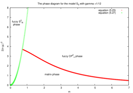
Figure 1: The phase diagram for the model $S_{0}$ with $\gamma=\frac{1}{12}$. In this case ${\phi}_{*}=1$ and hence the large mass expansion (5.23) becomes $\bar{\alpha}_{*}^{4}=\frac{108}{4m^{2}+27}$ while the small mass expansion (5.27) is $\bar{\alpha}_{*}^{4}=\frac{64}{9}m^{2}$ with $m=\hat{M}$. The intersection point occurs at $\hat{M}_{T}$. This looks like a triple point.

Acknowledgements

The work of D.D is supported by the College of Science-Research Center Project No: phys/2006/04.The work of D.Dou is also supported in part by the associate scheme of Abdus Salam ICTP. The work of Badis Ydri is supported by a Marie Curie Fellowship from The Commission of the European Communities ( The Research Directorate-General ) under contract number MIF1-CT-2006-021797. B.Y would like also to thank the staff at Humboldt-Universitat zu Berlin for their help and support. In particular he would like to thank Michael Muller-Preussker and Wolfgang Bietenholz.

Appendix A The one-loop effective action and effective potential for zero mass

First we can compute explicitly the following classical actions

$$Tr_{N}F_{ab}^{2}=Tr_{N}\bigg{(}-[D_{a},D_{b}]^{2}+4if_{abc}D_{a}D_{b}D_{c}+3D_{a}^{2}\bigg{)}.$$ (A.1)

$$Tr_{N}{\Phi}^{2}=\frac{1}{n^{2}}Tr_{N}\bigg{[}(D_{a}^{2})^{2}-\frac{2}{3}n(n+3)D_{a}^{2}+\frac{1}{9}n^{2}(n+3)^{2}\bigg{]}.$$ (A.2)

$$Tr_{N}{\Phi}_{a}^{2} = \frac{1}{n^{2}}Tr_{N}\bigg{[}\frac{1}{3}D_{a}D_{b}D_{a}D_{b}+\frac{1}{6}f_{aa^{{}^{\prime}}c}f_{bb^{{}^{\prime}}c}\{D_{a},D_{b}\}\{D_{a^{{}^{\prime}}},D_{b^{{}^{\prime}}}\}+\bigg{(}\frac{2n+3}{6}\bigg{)}^{2}D_{a}^{2}$$ (A.3)

$$- \frac{2n+3}{3}d_{abc}D_{a}D_{b}D_{c}\bigg{]}.$$

In above we have used the identity (2.5) and the identity

$$f_{abc}f_{abd}=3{\delta}_{cd}.$$ (A.4)

We can compute ( with $F_{ab}^{(0)}=F_{ab}-i[A_{a},A_{b}]$ )

$$S_{0}=\frac{1}{2g^{2}}Tr_{N}F_{ab}^{2}-\frac{1}{6g^{2}}f_{abc}Tr_{N}A_{c}F_{ab}-\frac{1}{12g^{2}}f_{abc}Tr_{N}A_{c}F_{ab}^{(0)}.$$ (A.5)

Next we will study the quantization of the action

$${S}_{i}[D,J] = S_{i}[D]+Tr_{N}J_{a}D_{a}\leavevmode\nobreak\ ,\leavevmode\nobreak\ S_{i}[D]=\bar{S}_{i}[D]+\bar{V}_{i}[D]$$ (A.6)

where

$$\bar{S}_{i}[D] = \frac{1}{g^{2}}Tr_{N}\bigg{(}-\frac{1}{4}[D_{a},D_{b}]^{2}+i{\alpha}_{i}f_{abc}D_{a}D_{b}D_{c}\bigg{)}$$

$$\bar{V}_{i}[D] = {\rho}_{i}Tr_{N}\Phi+V_{i}={\rho}_{i}Tr_{N}\Phi+{\beta}_{i}Tr_{N}{\Phi}^{2}+M_{i}^{2}Tr_{N}{\Phi}_{c}^{2}.$$ (A.7)

For $S_{0}=\bar{S}_{0}+\bar{V}_{0}$ we have ${\alpha}_{0}=\frac{2}{3}$, ${\rho}_{0}={\beta}_{0}=M_{0}=0$ while for $S_{1}=\bar{S}_{1}+\bar{V}_{1}$ we have ${\alpha}_{1}=1$, ${\rho}_{1}=\frac{3n}{4g^{2}}$, ${\beta}_{1}=\beta$ and $M_{1}=M$. $J_{a}$ is a source.

We adopt the background field method to the problem of quantization of this model. We write $D_{a}=B_{a}+Q_{a}$ where $B_{a}$ is the background field and $Q_{a}$ is the fluctuation field. We will fix the gauge by adding to the action the gauge-fixing and Fadeev-Popov terms, viz

$$S_{\rm g.fixing}+S_{\rm gh} = -\frac{1}{2g^{2}}\frac{1}{\xi}Tr_{N}[B_{a},Q_{a}]^{2}-Tr_{N}[B_{a},b^{+}][B_{a},b].$$ (A.8)

We compute

$$Tr_{N}[D_{a},D_{b}]^{2} = Tr_{N}\bigg{(}[B_{a},B_{b}]^{2}+2[B_{a},B_{b}][Q_{a},Q_{b}]+2[B_{a},Q_{b}]^{2}+2[B_{a},Q_{b}][Q_{a},B_{b}]$$ (A.9)

$$+ 4[B_{a},B_{b}][B_{a},Q_{b}]+O(Q^{3})\bigg{)}.$$

And

$$if_{abc}Tr_{N}D_{a}D_{b}D_{c} = if_{abc}Tr_{N}B_{a}B_{b}B_{c}+3if_{abc}Tr_{N}B_{a}B_{b}Q_{c}+3if_{abc}Tr_{N}Q_{a}Q_{b}B_{c}.$$ (A.10)

We find ( by using the identity $Tr_{N}[B_{a},Q_{b}][B_{b},Q_{a}]=Tr_{N}[B_{a},Q_{a}]^{2}-Tr_{N}[B_{a},B_{b}][Q_{a},Q_{b}]$ ) the following expression

$$\bar{S}_{i}[D] = \bar{S}_{i}[B]+\frac{i}{g^{2}}Tr_{N}\bigg{[}B_{ab}-(1-\frac{3{\alpha}_{i}}{2})f_{abc}B_{c},B_{a}\bigg{]}Q_{b}-\frac{1}{2g^{2}}Tr_{N}\bigg{(}[B_{a},Q_{b}]^{2}$$ (A.11)

$$- [B_{a},Q_{a}]^{2}+2iQ_{a}\bigg{[}B_{ab}-(1-\frac{3{\alpha}_{i}}{2})f_{abc}B_{c},Q_{b}\bigg{]}\bigg{)}+O(Q^{3})$$

$$= \bar{S}_{i}[B]+\frac{i}{g^{2}}Tr_{N}\bigg{[}B_{ab}-(1-\frac{3{\alpha}_{i}}{2})f_{abc}B_{c},B_{a}\bigg{]}Q_{b}+\frac{1}{2g^{2}}Tr_{N}Q_{a}\bigg{(}{\cal B}_{c}^{2}{\delta}_{ab}$$

$$- {\cal B}_{a}{\cal B}_{b}-2i{\cal B}_{ab}+2i(1-\frac{3{\alpha}_{i}}{2})f_{abc}{\cal B}_{c}\bigg{)}Q_{b}+O(Q^{3}).$$

$B_{ab}$ is the curvature of the background curvature $B_{a}$, in other words $B_{ab}=i[B_{a},B_{b}]+f_{abc}B_{c}$. Remark also how this action simplifies for $S_{0}$, i.e for ${\alpha}_{0}=\frac{2}{3}$. This “technical” simplification is a major advantage in considering $S_{0}$ instead of $S_{1}$. Given a matrix $O$ the operator ${\cal O}$ is given by ${\cal O}(..)=[O,..]$, for example ${\cal B}_{a}(Q_{a})=[B_{a},Q_{a}]$.

We can also compute

$${\rho}_{i}Tr_{N}\Phi={\rho}_{i}Tr_{N}\Psi+\frac{2{\rho}_{i}}{n}Tr_{N}B_{b}Q_{b}+\frac{{\rho}_{i}}{n}Tr_{N}Q_{a}^{2}.$$ (A.12)

$${\beta}_{i}Tr_{N}{\Phi}^{2} = {\beta}_{i}Tr_{N}{\Psi}^{2}+\frac{2{\beta}_{i}}{n}Tr_{N}\{B_{b},{\Psi}\}Q_{b}+\frac{{\beta}_{i}}{n^{2}}Tr_{N}Q_{a}\bigg{(}-{\cal B}_{a}{\cal B}_{b}+4B_{a}B_{b}+2n{\delta}_{ab}\Psi\bigg{)}Q_{b}$$ (A.13)

$$+ O(Q^{3}).$$

$$M_{i}^{2}Tr_{N}{\Phi}_{c}^{2} = M_{i}^{2}Tr_{N}{\Psi}_{c}^{2}+\frac{2M_{i}^{2}}{n}Tr_{N}\bigg{(}d_{abc}\{B_{b},{\Psi}_{c}\}-\frac{2n+3}{6}{\Psi}_{b}\bigg{)}Q_{b}$$ (A.14)

$$+ \frac{M_{i}^{2}}{n^{2}}Tr_{N}Q_{a}\bigg{(}-d_{aa^{{}^{\prime}}c}d_{bb^{{}^{\prime}}c}{\cal B}_{a^{{}^{\prime}}}{\cal B}_{b^{{}^{\prime}}}+4d_{aa^{{}^{\prime}}c}d_{bb^{{}^{\prime}}c}B_{a^{{}^{\prime}}}B_{b^{{}^{\prime}}}-2(\frac{2n+3}{3})d_{abc}B_{c}$$

$$+ 2nd_{abc}{\Psi}_{c}+(\frac{2n+3}{6})^{2}{\delta}_{ab}\bigg{)}Q_{b}+O(Q^{3}).$$

$\Psi$ and ${\Psi}_{c}$ are the normal scalar fields corresponding to the background covariant derivative $B_{a}$, viz ${\Psi}=\frac{1}{n}(B_{a}^{2}-|n|^{2})$ and ${\Psi}_{c}=\frac{1}{n}(d_{abc}B_{a}B_{b}-\frac{2n+3}{6}B_{c})$ where $|n|^{2}=\frac{1}{3}n(n+3)$.

Let us now introduce the actions ${S}_{i}[D,J]=\bar{S}_{i}[D]+\bar{V}_{i}[D]+Tr_{N}J_{a}D_{a}$ and ${S}_{i}[B,J]=\bar{S}_{i}[B]+\bar{V}_{i}[B]+Tr_{N}J_{a}B_{a}$. By using the above ingredients we have immediately the result

$${S}_{i}[D,J]+S_{\rm g.fixing}+S_{\rm gh} = {S}_{i}[B,J]+Tr_{N}{\cal J}_{b}^{i}Q_{b}+\frac{1}{2g^{2}}Tr_{N}Q_{a}{\Omega}_{ab}^{i}Q_{b}+O(Q^{3})$$ (A.15)

$$+ Tr_{N}b^{+}{\cal B}^{2}_{a}b.$$

In above ${\cal J}_{a}^{i}$ and ${\Omega}_{ab}^{i}$ are given respectively by

$${\cal J}_{b}^{i} = J_{b}+\frac{i}{g^{2}}[B_{ab}-(1-\frac{3{\alpha}_{i}}{2})f_{abc}B_{c},B_{a}]+\frac{2{\rho}_{i}}{n}B_{b}$$ (A.16)

$$+ \frac{2{\beta}_{i}}{n}\{B_{b},\Psi\}+\frac{2M_{i}^{2}}{n}(d_{abc}\{B_{b},{\Psi}_{c}\}-\frac{2n+3}{6}{\Psi}_{b})$$

$${\Omega}_{ab}^{i} = {\cal B}_{c}^{2}{\delta}_{ab}+(\frac{1}{\xi}-1){\cal B}_{a}{\cal B}_{b}-2i{\cal B}_{ab}+2i(1-\frac{3{\alpha}_{i}}{2})f_{abc}{\cal B}_{c}+\frac{2g^{2}{\rho}_{i}}{n}{\delta}_{ab}$$ (A.17)

$$+ \frac{2g^{2}{\beta}_{i}}{n^{2}}\bigg{(}-{\cal B}_{a}{\cal B}_{b}+4B_{a}B_{b}+2n{\delta}_{ab}\Psi\bigg{)}+\frac{2g^{2}M_{i}^{2}}{n^{2}}\bigg{(}-d_{aa^{{}^{\prime}}c}d_{bb^{{}^{\prime}}c}{\cal B}_{a^{{}^{\prime}}}{\cal B}_{b^{{}^{\prime}}}$$

$$+ 4d_{aa^{{}^{\prime}}c}d_{bb^{{}^{\prime}}c}B_{a^{{}^{\prime}}}B_{b^{{}^{\prime}}}-2(\frac{2n+3}{3})d_{abc}B_{c}+2nd_{abc}{\Psi}_{c}+(\frac{2n+3}{6})^{2}{\delta}_{ab}\bigg{)}.$$

In the following we will assume that the background fields $B_{a}$ satisfy the equations of motion ${\cal J}_{b}^{i}=0$ and we will choose the gauge ${\xi}^{-1}=1+\frac{2g^{2}{\beta}_{i}}{n^{2}}$. We then obtain

$${S}_{i}[D,J]+S_{\rm g.fixing}+S_{\rm gh} = {S}_{i}[B,J]+\frac{1}{2g^{2}}Tr_{N}Q_{a}{\Omega}_{ab}^{i}Q_{b}+O(Q^{3})+Tr_{N}b^{+}{\cal B}^{2}_{a}b.$$ (A.18)

The fluctuation fields $Q_{a}$ and the ghosts can be integrated out since they are Gaussian and one obtains therefore the effective action

$${\Gamma}_{i}[B,J] = {S}_{i}[B,J]+\frac{1}{2}Tr_{8}TR\log{\Omega}^{i}_{ab}-TR\log{\cal B}_{a}^{2}.$$ (A.19)

where

$${\Omega}_{ab}^{i} = {\cal B}_{c}^{2}{\delta}_{ab}-2i{\cal B}_{ab}+2i(1-\frac{3{\alpha}_{i}}{2})f_{abc}{\cal B}_{c}+\frac{2g^{2}{\rho}_{i}}{n}{\delta}_{ab}+\frac{2g^{2}{\beta}_{i}}{n^{2}}\bigg{(}4B_{a}B_{b}+2n{\delta}_{ab}\Psi\bigg{)}$$ (A.20)

$$+ \frac{2g^{2}M_{i}^{2}}{n^{2}}\bigg{(}-d_{aa^{{}^{\prime}}c}d_{bb^{{}^{\prime}}c}{\cal B}_{a^{{}^{\prime}}}{\cal B}_{b^{{}^{\prime}}}+4d_{aa^{{}^{\prime}}c}d_{bb^{{}^{\prime}}c}B_{a^{{}^{\prime}}}B_{b^{{}^{\prime}}}-2(\frac{2n+3}{3})d_{abc}B_{c}+2nd_{abc}{\Psi}_{c}$$

$$+ (\frac{2n+3}{6})^{2}{\delta}_{ab}\bigg{)}.$$

Now we compute the effective potential on fuzzy ${\bf CP}^{2}$ for $V_{0}=0$. For the configuration (4.2) we consider the following two cases

Case $1$

For $S_{0}$ we have ${\alpha}_{0}=\frac{2}{3}$ and ${\rho}_{0}=0$ and hence

$${\Gamma}_{0}[D]=\frac{3|n|^{2}}{g^{2}}\bigg{[}\frac{1}{4}{\phi}^{4}-\frac{1}{3}{\phi}^{3}\bigg{]}+\frac{1}{2}Tr_{8}TR\log{\Omega}^{0}_{ab}-TR\log{\phi}^{2}{\cal L}_{a}^{2}$$

$${\Omega}^{0}_{ab}={\phi}^{2}{\cal L}_{c}^{2}{\delta}_{ab}-{\phi}(\phi-1)\bigg{[}{\cal J}_{c}^{2}-{\cal L}_{c}^{2}-(Adt_{c})^{2}\bigg{]}_{ab}\leavevmode\nobreak\ ,\leavevmode\nobreak\ \vec{\cal J}=\vec{\cal L}+{Ad}\vec{t}.$$ (A.21)

The total $SU(3)$ angular momentum $\vec{\cal J}$ corresponds to the tensor product of the irreducible representations $(p,p)$ where $p=0,...,n$ ( corresponding to $\vec{\cal L}$ ) with the adjoint representation $(1,1)$ ( corresponding to $Ad\vec{t}$ ). By using Young tableaux we obtain the decomposition

$$(p,p){\otimes}(1,1) = (p+1,p+1)\oplus(p-1,p-1)\oplus(p,p)\oplus(p,p)\oplus(p-1,p+2)\oplus(p+2,p-1)$$ (A.22)

$$\oplus (p-2,p+1)\oplus(p+1,p-2).$$

The dimension of an irreducible representation $(n_{1},n_{2})$ of $SU(3)$ is $d(n_{1},n_{2})=\frac{1}{2}(n_{1}+1)(n_{2}+1)(n_{1}+n_{2}+2)$ and the quadratic Casimir is $c_{2}(n_{1},n_{2})=\frac{1}{3}(n_{1}^{2}+n_{1}n_{2}+3n_{1}+3n_{2}+n_{2}^{2})$. Thus we can immediately compute

$${\cal J}_{c}^{2}-{\cal L}_{c}^{2}-(Adt_{c})^{2}={\cal J}_{c}^{2}-(p^{2}+2p)-3={\rm diag}({2p},-(2p+4),-3,0,-p-3).$$ (A.23)

In this diagonal matrix the dimensions of the first block is $d(p+1,p+1)=(p+2)^{3}$, the second block is $d(p-1,p-1)=p^{3}$, the third block is $2d(p,p)=2(p+1)^{3}$, the $4$th block is $d(p-1,p+2)+d(p+2,p-1)=2d(p-1,p+2)=p(p+3)(2p+3)$ and the $5$th block is $d(p-2,p+1)+d(p+1,p-2)=2d(p-2,p+1)=(p-1)(p+2)(2p+1)$.

It is obvious from the above equation (A.23) that the second term in ${\Omega}$ is at most linear in $p$ while the first term is quadratic and hence in the large $n$ limit ( where large values of $p$ which are of the odrer of $n$ are expected to contribute the most ) we can make the approximation ${\Omega}_{ab}={\phi}^{2}{\cal L}_{c}^{2}{\delta}_{ab}$

Thus the quantum effective potential is

$${\Gamma}_{0}[D] = S_{0}[D]+\frac{1}{2}Tr_{8}TR\log({\phi}^{2}{\cal L}_{a}^{2}{\bf 1}_{8})-TR\log({\phi}^{2}{\cal L}_{a}^{2})$$ (A.24)

$$= \frac{3|n|^{2}}{g^{2}}\bigg{[}\frac{1}{4}{\phi}^{4}-\frac{1}{3}{\phi}^{3}\bigg{]}+\frac{1}{2}(8)(N^{2})\log{\phi}^{2}-(N^{2})\log{\phi}^{2}+{\rm constant}$$

$$= \frac{3|n|^{2}}{g^{2}}\bigg{[}\frac{1}{4}{\phi}^{4}-\frac{1}{3}{\phi}^{3}\bigg{]}+6N^{2}\log{\phi}+{\rm constant}.$$

Recall that $N=\frac{1}{2}(n+1)(n+2)$ and $|n|^{2}=\frac{1}{3}n(n+3)$ and hence

$$V_{\rm eff}=\frac{\Gamma[B]}{6N^{2}} = \frac{2}{3n^{2}g^{2}}\bigg{[}\frac{1}{4}{\phi}^{4}-\frac{1}{3}{\phi}^{3}\bigg{]}+\log{\phi}+{\rm constant}.$$ (A.25)

Case $2$

For $S_{1}$ we have ${\alpha}_{1}=1$ and ${\rho}_{1}=\frac{3n}{4g^{2}}$ and hence

$${\Omega}^{1}_{ab} = \bigg{(}{\phi}^{2}{\cal L}_{c}^{2}+\frac{3}{2}\bigg{)}{\delta}_{ab}+2i\phi(\phi-\frac{3}{2})f_{abc}{\cal L}_{c}.$$ (A.26)

The only difference ( as far as this quantum correction is concerned ) with case $1$ is that we have now a shifted Laplacian ${\phi}^{2}{\cal L}_{c}^{2}+\frac{3}{2}$ so the result for the determinant already obtained will not be altered. We end up thus with the effective potential

$$V_{\rm eff}=\frac{\Gamma[B]}{6N^{2}} = \frac{2}{3n^{2}g^{2}}\bigg{[}\frac{1}{4}{\phi}^{4}-\frac{1}{2}{\phi}^{3}+\frac{1}{4}{\phi}^{2}\bigg{]}+\log{\phi}+{\rm constant}.$$ (A.27)

References

- [1] Badis Ydri, Fuzzy Physics, PhD thesis (2001), hep-th/0110006.
- [2] H.Grosse,C.Klimčik,P.Pre šnajder,Commun.Math.Phys. 180 (1996) 429, Int.J.Theor.Phys. 35 (1996) 231. D.O’Connor, Mod.Phys.Lett. A18 (2003) 2423. C.Klimčik, Commun.Math.Phys. 199 (1998) 257. A. P. Balachandran, S. Kurkcuoglu and S. Vaidya,”Lectures on fuzzy and fuzzy SUSY physics”, hep-th/0511114 .
- [3] A. Connes, Noncommutative Geometry, Academic Press, London , 1994 . G. Landi, An introduction to noncommutative spaces and their geometry, springer (1997). J. M. Gracia-Bondia, J. C. Varilly, H. Figueroa, Elements of Noncommutative Geometry, Birkhauser (2000).
- [4] Brian P. Dolan, Idrish Huet, Sean Murray, Denjoe O’Connor, hep-th/0611209.
- [5] N. Ishibashi, H. Kawai, Y. Kitazawa, A. Tsuchiya, Nucl.Phys. B498 (1997) 467-491.
- [6] H. Aoki, S. Iso, H. Kawai, Y. Kitazawa, T. Tada, Prog.Theor.Phys. 99 (1998) 713-746. H. Aoki, S. Iso, H. Kawai, Y. Kitazawa, T. Tada, A. Tsuchiya, Prog.Theor.Phys.Suppl. 134 (1999) 47-83. H. Aoki, N. Ishibashi, S. Iso, H. Kawai, Y. Kitazawa, T. Tada, Nucl.Phys. B565 (2000) 176-192.
- [7] J.Madore,Class.Quant.Grav. 9:69-88,1992. J.Hoppe, MIT PhD thesis (1982). J.Hoppe, S.T.Yau, Commun.Math.Phys.195(1998)67-77.
- [8] S.Iso, Y.Kimura, K.Tanaka, K.Wakatsuki, Nucl.Phys. B604 (2001) 121.
- [9] P.Castro-Villarreal , R.Delgadillo-Blando , Badis Ydri , Nucl.Phys.B 704 (2004) 111-153.
- [10] T.Azuma , S.Bal, K.Nagao , J.Nishimura, hep-th/0405277.
- [11] D.O’Connor, Badis Ydri, hep-lat/0606013, JHEP11(12006)016.
- [12] Badis Ydri, Quantum equivalence of NC and YM gauge theories in 2D and matrix theory, hep-th/0701057. Badis Ydri , The one-plaquette model limit of NC gauge theory in 2D, hep-th/0606206, to be published in NPB.
- [13] A.Y.Alekseev , A.Recknagel, V.Schomerus, hep-th/0003187 and hep-th/9812193 .
- [14] P.Castro-Villarreal , R.Delgadillo-Blando , Badis Ydri, JHEP09 (2005)066. R.Delgadillo-Blando , Badis Ydri, Towards Noncommutative Fuzzy QED, hep-th/0611177.
- [15] A.P. Balachandran, S. Kurkcuoglu, Int.J.Mod.Phys.A19:3395-3408,2004. Luiz C. de Albuquerque, Paulo Teotonio-Sobrinho, Sachindeo Vaidya JHEP. 0410:024,2004.
- [16] J.Arnlind, M.Bordemann, L.Hofer, J.Hoppe, H.Shimada, hep-th/0602290.
- [17] G.Alexanian, A.P.Balachandran, G.Immirzi, B.Ydri, J.Geo.Phys.42 (2002) 28-53.
- [18] H.Grosse, A Strohmaier, Lett.Math.Phys. 48 (1999) 163-179.
- [19] A.P. Balachandran, Brian P. Dolan, J. Lee, X. Martin, Denjoe O’Connor, hep-th/0107099.
- [20] H.Grosse, H.Steinacker,hep-th/0407089.