HIP-2007-02/TH

hep-th/0701159

Dependence of SU(N) coupling behavior on the size of extra dimensions

Nobuhiro Uekusa

High Energy Physics Division, Department of Physical Sciences, University of Helsinki and Helsinki Institute of Physics, P.O. Box 64, FIN-00014 Helsinki, Finland

Coupling constants at high energy scales are studied in SU(N) gauge theory with distinct sizes of extra dimensions. We present the solution of gauge couplings as functions of the energy in such a way as to track the number of Kaluza-Klein modes. In a flat extra dimension, it is shown that the gauge couplings have logarithmic dependence on the size of the extra dimension and linear dependence on the number of Kaluza-Klein modes. We find some patterns of the dependence on flavor of bulk and brane fermions. Dependence of gauge couplings on the size of an extra dimension is discussed also in a warped extra dimension.

1 Introduction

There have been many attempts to study the effect of extra dimensions. Initial proposals for large extra dimensions [1] and warped extra dimensions [2] assume that all particles in the standard model are confined on a brane with four-dimensional world volume. For extra dimensions with the size smaller than the TeV scale, it is an interesting possibility that some fields are propagating in higher-dimensional bulk spacetime. In such various brane-world scenarios, it is possible for extra dimensions to have an effect far below unification scale or the Planck scale.

One of the remarkable extra-dimensional effects in brane-world scenario with bulk fields is in running of coupling constants. Higher-dimensional theory is non-renormalizable. However, it can be assumed that the contributions from the Kaluza-Klein (KK) states with masses larger than the scale of interest are decoupled from the theory, giving rise to an approximately renormalizable theory. In this approximation the corrections to the gauge couplings can be calculated. In case of flat extra dimensions, it has been shown that the appearance of extra dimensions accelerates the running of the gauge couplings, due to the power-law corrections [3, 4]. This has been studied in various models such as grand unification [5, 6, 7, 8, 9]. Possible solutions to the problem raised on non-calculable corrections from unknown ultraviolet physics have also been proposed in some scenarios [10, 11].

More recently, the running of gauge couplings has been studied in the universal extra dimension scenario where the extra dimension is accessed by all the standard model fields [12, 13]. In [14], it has been shown that the size of the extra dimension is constrained in order that the gauge couplings remain perturbative up to the scale where they tend to unify. This reveals the size of extra dimension to be regarded as a significant ingredient for running of gauge couplings in brane-world scenario.

In this paper, we will examine how coupling constants in SU(N) gauge theory behave at high energy scales, depending on the sizes of extra dimensions, where we will take into account not only bulk fields but also brane fields. Our approach is based on four-dimensional KK effective Lagrangian similar to [14]. The first KK excitation occurs at the scale $(\pi/l)$ where $l$ is the size of the extra dimension. Up to this scale the gauge coupling evolution has a contribution only from zero mode. Between $(\pi/l)$ and $(2\pi/l)$, the running is still logarithmic but beta functions are modified due to the first KK excitation. Whenever a KK threshold is crossed, beta functions are renewed. In such a way as to track the number of KK states, we will solve gauge couplings as functions of the energy using the background field method. While the problem of ultraviolet sensitivity is beyond the scope of this paper, our formulation will include possible localized kinetic terms.

We will also examine dependence of gauge couplings on the size of extra dimension in Randall-Sundrum spacetime. One-loop beta function of gauge couplings can be calculated in a five-dimensional regularization scheme with holographic guide [15]. Equations in such a calculation involve the curvature of $AdS_{5}$ denoted by $k$. As suggested in certain models [16, 17], the size of extra dimension can be stabilized in the unit of $k$. From this point of view, we will interpret $k$-dependent gauge couplings to be $l$-dependent and find an asymptotic solution for a gauge coupling in a form dependent on the size of extra dimension.

The paper is organized as follows. In Sec. 2, we will give Lagrangian for gauge fields and fermions in five-dimensional flat space and derive four-dimensional KK effective Lagrangian. After two kinds of gauge invariance in the theory will be shown, we will solve gauge couplings using the background field method. In Sec. 3, we will give an asymptotic solution for a gauge coupling dependent on the size of extra dimension. Summary and discussions will be given in Sec. 4.

2 A flat extra dimension

In this section, we will examine gauge couplings on the orbifold $S^{1}/Z_{2}$. Our notation assumes that gauge group SU(N) in four dimensions leaves unbroken, that all fermions are Dirac fermions and that there are $2N_{f}$ bulk fermions and $n_{f}$ brane fermions.

In this paper, capitalized indices $M,N$ run over 0,1,2,3,5, lower-case indices $m$ run over 0,1,2,3 and $(0),(n)$ are zero mode and KK mode indices where $n$ is a natural number. We use a timelike metric $\eta_{mn}=\textrm{diag}(1,-1,-1,-1)$ and take the following basis for the Dirac matrices

$$\gamma^{M}=\left(\left(\begin{array}[]{cc}0&\sigma^{m}\\ \bar{\sigma}^{m}&0\\ \end{array}\right),\left(\begin{array}[]{cc}-i&0\\ 0&i\\ \end{array}\right)\right),$$ (2.5)

where $\sigma^{m}=(1,\overrightarrow{\sigma})$, $\bar{\sigma}^{m}=(1,-\overrightarrow{\sigma})$.

2.1 Lagrangian and gauge invariance

We consider five-dimensional SU(N) gauge theory on the orbifold $S^{1}/Z_{2}$ with the metric

$$ds^{2}=g_{MN}dx^{M}dx^{N}=\eta_{mn}dx^{m}dx^{n}-dx^{5}dx^{5}.$$ (2.6)

Two branes are located at $x^{5}=0,l$. The five-dimensional starting Lagrangian is

$${\cal L}={\cal L}_{\textrm{\scriptsize gauge}}+{\cal L}_{\textrm{\scriptsize fermion}}.$$ (2.7)

The Lagrangian composed purely of the gauge field $A_{M}(x,x^{5})=A_{M}^{a}(x,x^{5})t^{a}$ is written as

$${\cal L}_{\textrm{\scriptsize gauge}}=-{1\over 4g^{2}}(F_{MN}^{a})^{2}-{1\over 4g_{1}^{2}}(F_{mn}^{a}{}_{(0)})^{2}\delta(x^{5})-{1\over 4g_{2}^{2}}(F_{mn}^{a}{}_{(0)})^{2}\delta(x^{5}-l),$$ (2.8)

with the field strength $F_{MN}^{a}=\partial_{M}A_{N}^{a}-\partial_{N}A_{M}^{a}+f^{abc}A_{M}^{b}A_{N}^{c}$, where $g,g_{1},g_{2}$ are the gauge coupling constants and $f^{abc}$ is the structure constant. The localized kinetic terms are denoted as the terms multiplied by the delta function. The Lagrangian for one-flavor bulk fermions is given by

$${\cal L}_{\textrm{\scriptsize fermion}}=\bar{\psi}^{i}(i\gamma^{M}D_{M})\psi^{i},$$ (2.9)

with $i=1,2$. The covariant derivative is $D_{M}=\partial_{M}-iA_{M}^{a}t^{a}$.

Let us derive the four-dimensional Lagrangian so that gauge coupling of zero mode can be calculated. By KK mode expansion, the gauge field is decomposed into

$$A_{m}^{a}(x,x^{5})=A_{m}^{a}{}_{(0)}(x)+\sum_{n=1}\sqrt{2}A_{m}^{a}{}_{(n)}(x)\cos({n\pi x^{5}\over l})$$ (2.10)

$$A_{5}^{a}(x,x^{5})=\sum_{n=1}\sqrt{2}A_{5}^{a}{}_{(n)}(x)\sin({n\pi x^{5}\over l}).$$ (2.11)

Substituting the KK mode expansion into the Lagrangian (2.8), we obtain the four-dimensional gauge part Lagrangian

$$\int_{0}^{l}~{}dx^{5}~{}{\cal L}_{\textrm{\scriptsize gauge}} \!\!=\!\! -{1\over 4g^{2}}(l+{g^{2}\over g_{1}^{2}}+{g^{2}\over g_{2}^{2}})(F_{mn}^{a}{}_{(0)})^{2}$$

$$-{l\over 4g^{2}}\sum_{n=1}\left((F_{mn}^{a}{}_{(n)})^{2}+2f^{abc}F_{mn}^{a}{}_{(0)}A^{mb}_{(n)}A^{nc}_{(n)}+2F_{m5}^{a}{}_{(n)}F^{m5a}_{(n)}\right).$$

The field strengths are given by

$$F_{mn}^{a}{}_{(0)} \!\!=\!\! \partial_{m}A_{n}^{a}{}_{(0)}-\partial_{n}A_{m}^{a}{}_{(0)}+f^{abc}A_{m}^{b}{}_{(0)}A_{n}^{c}{}_{(0)},$$

$$F_{mn}^{a}{}_{(n)} \!\!=\!\! \partial_{m}A_{n}^{a}{}_{(n)}-\partial_{n}A_{m}^{a}{}_{(n)}+f^{abc}A_{m}^{b}{}_{(m)}A_{n}^{c}{}_{(r)}\delta_{nmr}^{+}+f^{abc}(A_{m}^{b}{}_{(0)}A_{n}^{c}{}_{(n)}-A_{n}^{b}{}_{(0)}A_{m}^{c}{}_{(n)}),$$

$$F_{m5}^{a}{}_{(n)} \!\!=\!\! \partial_{m}A_{5}^{a}{}_{(n)}+({n\pi\over l})A_{m}^{a}{}_{(n)}+f^{abc}A_{m}^{b}{}_{(m)}A_{5}^{c}{}_{(r)}\delta_{nmr}^{-}+f^{abc}A_{m}^{b}{}_{(0)}A_{5}^{c}{}_{(n)},$$

with $\delta_{nmr}^{\pm}=(\delta_{n,m+r}+\delta_{m,n+r}\pm\delta_{r,n+m})/\sqrt{2}$. From Eqs.(LABEL:lag4d) and (LABEL:fm5), it is seen that the $n$-th KK gauge field $A_{m}^{a}{}_{(n)}$ has the mass $(n\pi/l)$. The $n$-th KK gauge field begins to play a dynamical role at energy scales higher than $(n\pi/l)$. We treat the summation over KK modes in the Lagrangian (LABEL:lag4d) as scale-dependent. This is explicitly written as $\sum_{n=1}^{m}$ at the energy range $m\pi/l\leq E<(m+1)\pi/l$. At scales less than $(\pi/l)$, the Lagrangian describes only zero mode as the summation is simply zero. The $n$-th KK scalar $A_{5}^{a}{}_{(n)}$ has the same mass as that of the $n$-th KK gauge field, as more explicitly seen after gauge fixing. The summation over the KK modes is treated similarly to the KK gauge field case.

The four-dimensional Lagrangian (LABEL:lag4d) is invariant under a standard four-dimensional gauge transformation. The infinitesimal gauge transformation law for $A_{m}^{a}{}_{(0)}$ is given by

$$\delta A_{m}^{a}{}_{(0)}=\partial_{m}\alpha^{a}+f^{abc}A_{m}^{b}{}_{(0)}\alpha^{c}$$ (2.14)

where $\alpha^{a}(x)$ is an infinitesimal parameter dependent on four-dimensional coordinates. The KK gauge field and scalar are transformed as adjoint matter fields,

$$\delta A_{m}^{a}{}_{(n)} \!\!=\!\! f^{abc}A_{m}^{b}{}_{(n)}\alpha^{c},$$ (2.15)

$$\delta A_{5}^{a}{}_{(n)} \!\!=\!\! f^{abc}A_{5}^{b}{}_{(n)}\alpha^{c}.$$ (2.16)

In addition to the standard gauge invariance, the Lagrangian (LABEL:lag4d) is also invariant under another gauge transformation with the infinitesimal local parameter $\alpha^{a}_{(n)}(x)$,

$$\delta_{(n)}A_{m}^{a}{}_{(0)}=0,$$ (2.17)

$$\delta_{(n)}A_{m}^{a}{}_{(n)}=\partial_{m}\alpha^{a}_{(n)}+f^{abc}A_{m}^{b}{}_{(m)}\alpha^{c}_{(r)}\delta_{nmr}^{+}+f^{abd}A_{m}^{b}{}_{(0)}\alpha^{c}_{(n)},$$ (2.18)

$$\delta_{(n)}A_{5}^{a}{}_{(n)}=-({n\pi\over l})\alpha_{(n)}^{a}+f^{abc}A_{5}^{b}{}_{(m)}\alpha^{c}_{(r)}\delta_{nmr}^{-}.$$ (2.19)

Using these two kinds of gauge invariance, we will choose gauge fixing convenient for the background field method.

Let us consider fermionic part. In order to calculate running of gauge coupling constant, we concentrate on quadratic fermionic Lagrangian. The $Z_{2}$ projection for the fermion fields is defined as

$$\left\{\begin{array}[]{l}\psi^{1}(x,-x^{5})=i\gamma_{5}\psi^{1}(x,x^{5}),\\ \psi^{1}(x,-x^{5}+l)=i\gamma_{5}\psi^{1}(x,x^{5}+l),\\ \end{array}\right.~{}~{}\left\{\begin{array}[]{l}\psi^{2}(x,-x^{5})=-i\gamma_{5}\psi^{2}(x,x^{5}),\\ \psi^{2}(x,-x^{5}+l)=-i\gamma_{5}\psi^{2}(x,x^{5}+l).\\ \end{array}\right.$$ (2.24)

From this parity assignment and the chiral representation $\psi^{i}=(\phi^{i}_{L},\phi^{i}_{R})^{T}$, the fermion fields are decomposed into

$$\phi_{L}^{1}(x,x^{5}) \!\!=\!\! {1\over\sqrt{l}}\psi_{L}(x)+\sum_{n=1}\sqrt{2\over l}\phi_{L}^{1}{}_{(n)}(x)\cos({n\pi x^{5}\over l}),$$ (2.25)

$$\phi_{R}^{1}(x,x^{5}) \!\!=\!\! \sum_{n=1}\sqrt{2\over l}\phi_{R}^{1}{}_{(n)}(x)\sin({n\pi x^{5}\over l}),$$ (2.26)

$$\phi_{L}^{2}(x,x^{5}) \!\!=\!\! \sum_{n=1}\sqrt{2\over l}\phi_{L}^{2}{}_{(n)}(x)\sin({n\pi x^{5}\over l}),$$ (2.27)

$$\phi_{R}^{2}(x,x^{5}) \!\!=\!\! {1\over\sqrt{l}}\psi_{R}(x)+\sum_{n=1}\sqrt{2\over l}\phi_{R}^{2}{}_{(n)}(x)\cos({n\pi x^{5}\over l}).$$ (2.28)

Writing four-dimensional Dirac fermions as

$$\psi=\left(\begin{array}[]{l}\psi_{L}\\ \psi_{R}\end{array}\right),~{}~{}\psi^{i}_{(n)}=\left(\begin{array}[]{l}\phi_{L}^{i}{}_{(n)}\\ \phi_{R}^{i}{}_{(n)}\end{array}\right),$$ (2.33)

we obtain four-dimensional fermionic Lagrangian

$$\int_{0}^{l}~{}dx^{5}~{}{\cal L}_{\textrm{\scriptsize fermion}}\bigg{|}_{\textrm{\scriptsize quad}} \!\!=\!\! \bar{\psi}(i\gamma^{m}\partial_{m})\psi$$

$$+\sum_{n=1}\bar{\psi}^{1}_{(n)}\left(i\gamma^{m}\partial_{m}-{n\pi\over l}\right)\psi^{1}_{(n)}+\sum_{n=1}\bar{\psi}^{2}_{(n)}\left(i\gamma^{m}\partial_{m}+{n\pi\over l}\right)\psi^{2}_{(n)}.$$

The summation over KK modes is treated as scale-dependent similarly to the KK gauge and scalar. The Lagrangian for $2N_{f}$ bulk fermions are obtained as the number of the Lagrangian (LABEL:lag4df) is $N_{f}$. The Lagrangian for $n_{f}$ brane fermions are obtained as the number of the first term in the right hand side of (LABEL:lag4df) is $n_{f}$.

2.2 Solution of gauge couplings

We have set up the four-dimensional effective Lagrangian with a scale-dependent KK mode summation. Now we apply the background field method to the Lagrangians (LABEL:lag4d) and (LABEL:lag4df). The zero mode gauge field is decomposed into classical background and quantum fluctuation

$$A_{m}^{a}{}_{(0)}\to A_{m}^{a}{}_{(0)}+{\cal A}_{m}^{a}.$$ (2.35)

The KK gauge field and scalar are interpreted as quantum fluctuation around zero classical background. Then the field strengths in (LABEL:fm5) become

$$F_{mn}^{a}{}_{(0)} \!\!\to\!\! F_{mn}^{a}{}_{(0)}+D_{m}{\cal A}_{n}^{a}-D_{n}{\cal A}_{m}^{a}+f^{abc}{\cal A}_{m}^{b}{\cal A}_{n}^{c},$$

$$F_{mn}^{a}{}_{(n)} \!\!\to\!\! F_{mn}^{a}{}_{(n)}+f^{abc}(A_{m}^{b}{}_{(n)}{\cal A}_{n}^{c}-A_{n}^{b}{}_{(n)}{\cal A}_{m}^{c}),$$ (2.36)

$$F_{m5}^{a}{}_{(n)} \!\!\to\!\! F_{m5}^{a}{}_{(n)}-f^{abc}A_{5}^{b}{}_{(n)}{\cal A}_{m}^{c},$$

where $D_{m}$ is the covariant derivative with respect to the background gauge field $A_{m}^{a}{}_{(0)}$. Since the four-dimensional Lagrangian has gauge invariance for the transformation parameters $\alpha^{a}$ and $\alpha_{(n)}^{a}$, we need to introduce two types of gauge fixing in order to define the functional integral. For the parameter $\alpha^{a}$, the gauge fixing function can be chosen as

$$G^{a}=\sqrt{1+{g^{2}\over lg^{2}_{1}}+{g^{2}\over lg^{2}_{2}}}\,D^{m}{\cal A}_{m}^{a}-\omega^{a}(x)$$ (2.37)

with a Gaussian weight for $\omega^{a}$. The corresponding ghost and antighost are denoted as $c$ and $\bar{c}$, respectively. For the other parameter $\alpha_{(n)}^{a}$, we choose the other gauge fixing function so as to cancel $A_{m}{}_{(n)}$-$A_{5}{}_{(n)}$ mixing terms in kinetic Lagrangian,

$$G^{a}_{(n)}=D^{m}A_{m}^{a}{}_{(n)}-\left({n\pi\over l}\right)A_{5}^{a}{}_{(n)}-\omega^{a}_{(n)},$$ (2.38)

with a Gaussian weight for $\omega^{a}_{(n)}$. The corresponding ghost and antighost are denoted as $c_{(n)}$ and $\bar{c}_{(n)}$, respectively. With these two types of gauge fixing functions, total quadratic Lagrangian is obtained as

$${\cal L}_{\textrm{\scriptsize quad}}={\cal L}_{\cal A}+{\cal L}_{n}+{\cal L}_{5}+{\cal L}_{c}+{\cal L}_{\psi},$$ (2.39)

$${\cal L}_{\cal A} \!\!=\!\! -{1\over 2g^{2}}\left(l+{g^{2}\over g_{1}^{2}}+{g^{2}\over g_{2}^{2}}\right)\left\{{1\over 2}(D_{m}{\cal A}_{n}^{a}-D_{n}{\cal A}_{m}^{a})^{2}\right.$$ (2.40)

$$\qquad\qquad\qquad\qquad\qquad\qquad\left.+f^{abc}F^{a}_{mn}{}_{(0)}{\cal A}^{mb}{\cal A}^{nc}+(D^{m}{\cal A}_{m}^{a})^{2}\right\},$$

$${\cal L}_{n} \!\!=\!\! -{l\over 2g^{2}}\left\{{1\over 2}(D_{m}A_{n}^{a}{}_{(n)}-D_{n}A_{m}^{a}{}_{(n)})^{2}-\left({n\pi\over l}\right)^{2}A_{m}^{a}{}_{(n)}A^{ma}_{(n)}\right.$$ (2.41)

$$\qquad\qquad\qquad\qquad\qquad\qquad\left.+f^{abc}F^{a}_{mn}{}_{(0)}A^{mb}_{(n)}A^{nc}_{(n)}+(D^{m}A_{m}^{a}{}_{(n)})^{2}\right\},$$

$${\cal L}_{5} \!\!=\!\! {l\over 2g^{2}}\left\{(D^{m}A_{5}^{a}{}_{(n)})(D_{m}A_{5}^{a}{}_{(n)})-\left({n\pi\over l}\right)^{2}A_{5}^{a}{}_{(n)}A_{5}^{a}{}_{(n)}\right\},$$ (2.42)

$${\cal L}_{c} \!\!=\!\! -i\sqrt{1+{g^{2}\over lg_{1}^{2}}+{g^{2}\over lg_{2}^{2}}}~{}\bar{c}^{a}(D^{2})^{ac}c^{c}-i~{}\bar{c}^{a}{}_{(n)}(D^{2}+\left({n\pi\over l}\right)^{2})^{ac}c_{(n)}^{c},$$ (2.43)

$${\cal L}_{\psi} \!\!=\!\! \bar{\psi}(i\gamma^{m}D_{m})\psi+\bar{\psi}^{1}_{(n)}\left(i\gamma^{m}D_{m}-{n\pi\over l}\right)\psi^{1}_{(n)}+\bar{\psi}^{2}_{(n)}\left(i\gamma^{m}D_{m}+{n\pi\over l}\right)\psi^{2}_{(n)}.$$ (2.44)

with summation over KK modes and flavor.

We now calculate gauge coupling constants in such a way to track the number of KK modes. For scales less than the mass of the first KK mode, the gauge coupling constant $\alpha^{-1}\equiv 4\pi g^{-2}(l+g^{2}g_{1}^{-2}+g^{2}g_{2}^{-2})$ is given by

$$\alpha^{-1}(E)=\alpha^{-1}(M)+{b\over 2\pi}\log{M\over E},~{}\quad\textrm{for}~{}~{}E<{\pi\over l},$$ (2.45)

where $E$ and $M$ are the scale of interest and another scale. In Eq.(2.45), $b$ is obtained only from zero mode part in the gauge-fixed Lagrangian (2.39) as

$$b=-\left({11\over 3}C_{2}(G)-{4\over 3}(N_{f}+n_{f})C(r)\right),$$ (2.46)

with $C_{2}(G)=N$ and $C(r)={1\over 2}$. The contributions to the factor $b$ from each field is tabulated in Table 1. As scales cross the mass of the first KK excitation, the first KK mode becomes dynamical. Then $\alpha^{-1}$ is given by

$$\alpha^{-1}(E)=\alpha^{-1}(M)+{b\over 2\pi}\log{M\over E}+{b_{\textrm{\scriptsize KK}}\over 2\pi}\log{\pi\over El},~{}\quad\textrm{for}~{}~{}{\pi\over l}\leq E<{2\pi\over l},$$ (2.47)

where

$$b_{\textrm{\scriptsize KK}}=-\left({21\over 6}C_{2}(G)-{8N_{f}\over 3}C(r)\right).$$ (2.48)

The contributions to $b_{\textrm{\scriptsize KK}}$ from each field is tabulated in Table 1.

Table 1: Contributions to $b$ and $b_{\textrm{\scriptsize KK}}$

(i) Zero mode contributes to $b$
Dirac	gauge	ghost
$\psi$	$A_{m}{}_{(0)}$	$c,\bar{c}$
${4(N_{f}+n_{f})C(r)\over 3}$	$-{10C_{2}(G)\over 3}$	$-{C_{2}(G)\over 3}$

(ii) KK mode contributes to $b_{\textrm{\scriptsize KK}}$
Dirac	gauge	scalar	ghost
$\psi^{i}{}_{(n)}$	$A_{m}{}_{(n)}$	$A_{5}{}_{(n)}$	$c_{(n)},\bar{c}{}_{(n)}$
${8N_{f}C(r)\over 3}$	$-{10C_{2}(G)\over 3}$	${C_{2}(G)\over 6}$	$-{C_{2}(G)\over 3}$

As scales are higher than the $n$-th KK mass, the first $n$ KK modes become dynamical. In this way, we find a general solution for $\alpha^{-1}$,

$$\alpha^{-1}(E) \!\!=\!\! \alpha^{-1}(M)+{b\over 2\pi}\log{M\over E}+{b_{\textrm{\scriptsize KK}}\over 2\pi}\sum_{m=1}^{n}\log{m\pi\over El}$$

$$\!\!=\!\! \alpha^{-1}(M)+{b\over 2\pi}\log{M\over E}+{b_{\textrm{\scriptsize KK}}\over 2\pi}\left(n\log{\pi\over El}+\log n!\right),~{}\textrm{for}~{}~{}{n\pi\over l}\leq E<{(n+1)\pi\over l}.$$

From this equation, it is seen that the gauge coupling has a linear dependence on KK level $n$ and a logarithmic dependence on size of extra dimension $l$. Behavior of the $\alpha^{-1}$ is schematically shown in Fig 1.

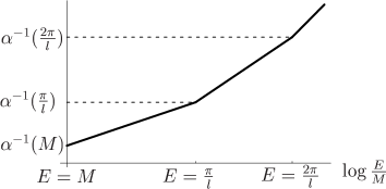
Figure 1: Behavior of a coupling is schematically drawn.

Below the scale of the appearance of the extra dimension, the gauge coupling has the contribution only from zero mode and the slope is $-b/(2\pi)$ for $\log E$. At $E=\pi/l$ where the first KK excitation occurs, the gauge coupling begins to have the slope $-(b+b_{\textrm{\scriptsize KK}})/(2\pi)$. Whenever scales cross a KK mass, the new KK mode with the mass is added and at $n\pi/l\leq E<(n+1)l/\pi$ the slope has $-(b+nb_{\textrm{\scriptsize KK}})/(2\pi)$. Unless $|b|\gg|b_{\textrm{\scriptsize KK}}|$, the running of the gauge coupling is strongly sensitive to the number of KK modes once the extra dimension appears with a size. For example, if the size of extra dimension is $l^{-1}=10^{5}$ GeV$/\pi$, the first 100 KK modes linearly would enhance the gauge coupling at the scale of $10^{7}$ GeV$/\pi$.

In order to find more specific patterns, we choose the numbers of flavor and color as well as the size of extra dimension as $N_{f}=6,3,0$, $n_{f}=6,3,0$, $N=2,3$ and $l^{-1}=10^{4},10^{10},10^{16}$ [GeV$/\pi$]. And we fix the total number of flavor as $N_{f}+n_{f}=6$. Behavior of the gauge coupling as a function of the energy is shown in Fig. 2.

(i)  $(N_{f},n_{f})=(6,0)$.

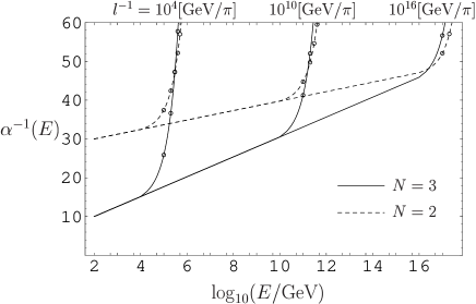
(ii)  $(N_{f},n_{f})=(3,3)$.

(iii)  $(N_{f},f_{f})=(0,6)$.

Figure 2: Behavior of the coupling as a function of the energy. Circles show the appearance of the ($10n$)-th KK mode where $n$ is a natural number. At $E=M(=100\textrm{GeV})$, the coupling constants are chosen as $\alpha^{-1}=10$ and 30 for $N=3$ and 2.

In the figure, the appearance of KK modes is shown with circles. As mentioned above, after the appearance of the extra dimension the gauge coupling increasingly evolves by including KK modes. An indication of the coupling evolution can be the energy when the gauge couplings for $N=2,3$ has the same value. At this energy, there is the same number of KK modes for $N=2,3$ since KK masses are independent of color. Defining the number of the KK modes as $n_{*}$ and the energy at a coincident point of gauge couplings as $E_{*}$, we find from Eq.(LABEL:generalsol)

$$E_{*}={\pi\over l}\left((n!)^{\Delta b_{k}}\left({Ml\over\pi}\right)^{\Delta b}e^{2\pi\Delta\alpha^{-1}}\right)^{1/\Delta b+n\Delta b_{k}}~{}\textrm{for}~{}~{}{n_{*}\pi\over l}\leq E_{*}<{(n_{*}+1)\pi\over l},$$ (2.50)

where $\Delta b_{k}=b_{\textrm{\scriptsize KK}\,N=2}-b_{\textrm{\scriptsize KK}\,N=3}$, $\Delta b=b_{N=2}-b_{N=3}$ and $\Delta\alpha^{-1}=\alpha^{-1}(M)_{N=2}-\alpha^{-1}(M)_{N=3}$. When the total number of flavor is fixed, dependence of $E_{*}$ on flavor occurs only due to $\Delta b_{k}$. If $N_{f}$ with fixed ($N_{f}+n_{f}$) is chosen as independent of color, $\Delta b_{k}$ becomes independent of flavor. Then the energy at a coincident point of gauge couplings is determined independently the value of $N_{f}$. In each case of $(N_{f},n_{f})$, $E_{*}$ is shown in Table 2.

Table 2: Energies at the coincident points of the gauge couplings in the unit of GeV. In each box, three quantities are denoted as the energies for $l^{-1}=10^{4},10^{10},10^{16}$[GeV/$\pi$] from above. For three cases shown in left-bottom boxes there is no solution.

As seen also from Fig. 2, there is no solution in the case where $N_{f}{}_{N=2}<N_{f}{}_{N=3}$. For $N_{f}{}_{N=2}\geq N_{f}{}_{N=3}$, as $N_{f}{}_{N=3}$ increases, the energy $E_{*}$ tends to increase. This is because the relative sign between bosons and fermions in the $b_{\textrm{\scriptsize KK}}$ (2.48) makes the evolution less for larger $N_{f}$. For $N_{f}{}_{N=2}=N_{f}{}_{N=3}$, $N_{f}$-value-independence of $E_{*}$ is seen in diagonal boxes in Table 2. In diagonal boxes and upper right boxes along them, it is also seen that $E_{*}$ is characterized by $(N_{f}{}_{N=2}-N_{f}{}_{N=3})$. These features of $E_{*}$ can be read in the view of the number of KK modes from the fact that $n_{*}$ is a maximum integer less than $E_{*}l/\pi$. The maximum number of $n_{*}$ is obtained for $N_{f}{}_{N=2}=N_{f}{}_{N=3}$ and largest $N_{f}{}_{N=3}$. From Table 2, it is seen that the number of KK modes for coinciding of the couplings is at most 30, 16, 2 for $l^{-1}=10^{4},10^{10},10^{16}$[GeV$/\pi$], respectively. Similar behavior is obtained for more general two gauge groups.

3 A warped extra dimension

In this section, we consider SU(N) gauge theory in the Randall-Sundrum geometry with metric

$$ds^{2}=g_{MN}dx^{M}dx^{N}={1\over(kz)^{2}}(\eta_{mn}dx^{m}dx^{n}-dz^{2}).$$ (3.1)

For simplicity, we consider purely gauge part

$${\cal S}=\int d^{4}xdz\sqrt{-\textrm{det}(g_{MN})}\left(-{1\over 4g^{2}}(F_{MN}^{a})^{2}\right).$$ (3.2)

As mentioned in Introduction, one-loop beta function of gauge couplings can be calculated in a five-dimensional regularization scheme. With the background field method, the gauge coupling is obtained as [15]

$$\alpha^{-1}(E)=\alpha^{-1}(M)+{b_{w}\over 2\pi}\log{M\over E},$$ (3.3)

$$b_{w}=-C_{2}(G)\left({11\over 3}I^{1,0}(0,\Lambda/k)-{1\over 6}I^{1,i}(0,\Lambda/k)\right),$$ (3.4)

where

$$I^{1,\nu}(y_{1},y_{2})=2\int_{y_{1}}^{y_{2}}ydy\int_{y}^{y_{2}}zdz\left({(AK_{\nu}(y)+BI_{\nu}(y))(CK_{\nu}(z)+DI_{\nu}(z))\over AD-BC}\right)^{2},$$ (3.5)

$$A \!\!=\!\! y_{1}I_{\nu-1}(y_{1})-(\nu-1)I_{\nu}(y_{1}),$$ (3.6)

$$B \!\!=\!\! y_{1}K_{\nu-1}(y_{1})-(\nu-1)K_{\nu}(y_{1}),$$ (3.7)

$$C \!\!=\!\! y_{2}I_{\nu-1}(y_{2})-(\nu-1)I_{\nu}(y_{2}),$$ (3.8)

$$D \!\!=\!\! y_{2}K_{\nu-1}(y_{2})-(\nu-1)K_{\nu}(y_{2}).$$ (3.9)

Now we calculate asymptotic form of the gauge coupling for $k\ll\Lambda$. The modified Bessel function $K_{\nu}$ is singular at $y_{1}\to 0$ so we will take limit $y_{1}\to 0$ after integral is performed. Throughout this analysis, we take into account $y_{1}\ll 1$ and $y_{2}\gg 1$. We also introduce $y_{3}$ such that $1\ll y_{3}\ll y_{2}$ and split the integral region into

$$\int_{y_{1}}^{y_{2}}=\int_{y_{1}}^{y_{3}}+\int_{y_{3}}^{y_{2}},~{}~{}\int_{y}^{y_{2}}=\int_{y}^{y_{3}}+\int_{y_{3}}^{y_{2}}.$$ (3.10)

Then Eq.(3.5) is approximated as

$$I^{1,\nu}(y_{1},y_{2})\approx{\cal I}_{1}+{\cal I}_{2},$$ (3.11)

where

$${\cal I}_{1} \!\!=\!\! 2\int_{y_{1}}^{y_{3}}ydy\int_{y_{3}}^{y_{2}}zdz\left({(AK_{\nu}(y)+BI_{\nu}(y))(CK_{\nu}(z)+DI_{\nu}(z))\over AD-BC}\right)^{2},$$ (3.12)

$${\cal I}_{2} \!\!=\!\! 2\int_{y_{3}}^{y_{2}}ydy\int_{y}^{y_{2}}zdz\left({(AK_{\nu}(y)+BI_{\nu}(y))(CK_{\nu}(z)+DI_{\nu}(z))\over AD-BC}\right)^{2}.$$ (3.13)

With the relation

$$AD\ll BC,~{}~{}AK_{\nu}(y)\ll BI_{\nu}(y)~{}~{}\textrm{for~{}large}~{}y$$ (3.14)

and modified Bessel function formula given in Appendix, the integrals are performed as

$${\cal I}_{1} \!\!=\!\! {2\over(AD-BC)^{2}}$$

$$\!\!\!\!\!\!\times\left[{y^{2}\over 2}((AK_{\nu}(y)+BI_{\nu}(y))^{2}-(AK_{\nu-1}(y)-BI_{\nu-1}(y))(AK_{\nu+1}(y)-BI_{\nu+1}(y)))\right]_{y_{1}}^{y_{3}}$$

$$\!\!\!\!\!\!\times\left[{z^{2}\over 2}((CK_{\nu}(z)+DI_{\nu}(z))^{2}-(CK_{\nu-1}(z)-DI_{\nu-1}(z))(CK_{\nu+1}(z)-DI_{\nu+1}(z)))\right]_{y_{3}}^{y_{2}},$$

$${\cal I}_{2} \!\!\approx\!\! 2\int_{y_{3}}^{y_{2}}ydy\int_{y}^{y_{2}}zdz\left(I_{\nu}(y)(K_{\nu}(z)+{D\over C}I_{\nu}(z))\right)^{2}.$$ (3.16)

For $y_{1}\to 0$ and $1\ll y_{3}\ll y_{2}$, one can show that these equations become

$${\cal I}_{1}\to 0,\qquad{\cal I}_{2}\approx{1\over 4}\,y_{2}.$$ (3.17)

Thus we obtain

$$I^{1,\nu}(0,\Lambda/k)={1\over 4}~{}{\Lambda\over k}.$$ (3.18)

The value given in Eq.(3.18) is close to $(1/\pi)(\Lambda/k)$ which is the number of KK modes below cut off estimated in [15]. To this extent, picture of KK effective theory works as an intuitive view. It is also possible to find dependence of the beta function on the size of the extra dimension. If a large cutoff $E=\Lambda$ is introduced into analysis in the previous section, the beta function would have linear dependence on $n\sim\pi(\Lambda l)$. Eq.(3.18) implies that when $kl$ is stabilized the beta function $b_{w}$ has linear dependence on $\Lambda l$, which is similar to KK picture.

4 Summary and discussions

We have examined how coupling constants in SU(N) gauge theory behave at high energy scales, depending on the sizes of extra dimensions. In a flat extra dimension, based on KK picture, we have solved gauge couplings as functions of the energy and have present a general equation. It has been shown that the gauge couplings have logarithmic dependence on the size of the extra dimension and linear dependence on the number of KK modes. The running of the gauge coupling can be sensitive to the number of KK modes once the extra dimension appears with any size. For example, the first 10 KK modes linearly would enhance the gauge coupling at an order of magnitude larger than the scale $\pi/l$.

In order to find some possible patterns of the coupling evolution dependent on flavor of bulk and brane fermions, we have also examined the energy when the couplings for two gauge group has the same value. It has been found that the energy at a coincident point of the two gauge couplings is independent of the value of the number of flavor if the number of flavor for one gauge group is the same as that of the other gauge group. For color $N=2,3$, if flavor of bulk fermions satisfies $N_{f}{}_{N=2}\geq N_{f}{}_{N=3}$ (with fixed total number of flavor), there exists such an energy. And as $N_{f}{}_{N=3}$ increase, the energy tends to be larger. This is because the relative sign between bosons and fermions in the $b_{\textrm{\scriptsize KK}}$ makes the evolution less for larger $N_{f}$. By our formulation, the energy at a coincident point is immediately translated into the KK level included in the evolution until the coincident point. As the size of the extra dimension is larger, the number of KK modes required for coinciding becomes larger. For $N=2,3$, the number of KK modes required is at most of order of ${\cal O}(10)$.

We have also given an asymptotic solution of a gauge coupling in Randall-Sundrum spacetime. From this solution and estimation about the number of KK modes below cut off in [15], picture of KK effective theory has been found to work to some extent as an intuitive view. Dependence of couplings on the size of the extra dimension has been given with a concept of stabilized $kl$.

It would be interesting to apply our solution and formulation in the context of gauge symmetry breaking, grand unification and supersymmetry. We have considered the case where all fields have the same KK mass. It would be straightforward to solve gauge couplings in models with field-dependent KK masses. The value of the gauge couplings itself depends strongly on field content. On the other hand, the number of KK modes required for coinciding of gauge coupling can be at most ${\cal O}(10)$, depending weakly on field content. The energy at a coincident point can be one to two orders of magnitude larger than $\pi/l$.

Acknowledgments

The author thanks Masud Chaichian for reading the manuscript. This work is supported by Bilateral exchange programme between the Academy of Finland and the Japanese Society for Promotion of Science.

Appendix A Integrals and asymptotic forms of modified Bessel functions

Integrals of functions including the modified Bessel functions $I_{\nu}$ and $K_{\nu}$ are shown in Table 3.

Table 3: Integrals including $I_{\nu}$ and $K_{\nu}$.

functions	indefinite integrals
$yI_{\nu}^{2}(z)$	${z^{2}\over 2}(I_{\nu}^{2}(z)-I_{\nu-1}(z)I_{\nu+1}(z))$
$yK_{\nu}^{2}(z)$	${z^{2}\over 2}(K_{\nu}^{2}(z)-K_{\nu-1}(z)K_{\nu+1}(z))$
$yI_{\nu}(z)K_{\nu}(z)$	${z^{2}\over 2}(I_{\nu}(z)K_{\nu}(z)+{1\over 2}(I_{\nu-1}(z)K_{\nu+1}(z)+I_{\nu+1}(z)K_{\nu-1}(z)))$

At the leading order, $I_{\nu}$ and $K_{\nu}$ are independent of $\nu$ for large $|z|$,

$$I_{\nu}(z)\approx{e^{z}\over\sqrt{2\pi z}},~{}~{}K_{\nu}(z)\approx\sqrt{\pi\over 2z}e^{-z},$$ (A.1)

and for small $z$,

$$I_{\nu}(z)\approx\left({z\over 2}\right)^{\nu}{1\over\Gamma(\nu+1)},~{}~{}K_{\nu}(z)\approx\left({z\over 2}\right)^{-\nu}{\Gamma(\nu)\over 2},$$ (A.2)

for $\nu=n$ ($n$ is non-negative integer)

$$K_{n}(z)=K_{-n}(z)\approx\left\{\begin{array}[]{l}-\log z~{}~{}\qquad\qquad\textrm{for}~{}n=0\\ {1\over 2}(n-1)!\left({z\over 2}\right)^{-n}~{}~{}\textrm{for}~{}n\neq 0.\\ \end{array}\right.$$ (A.5)

References

- [1] I. Antoniadis, Phys. Lett. B 246, 377 (1990); N. Arkani-Hamed, S. Dimopoulos and G. R. Dvali, Phys. Lett. B 429, 263 (1998) [arXiv:hep-ph/9803315]; I. Antoniadis, N. Arkani-Hamed, S. Dimopoulos and G. R. Dvali, Phys. Lett. B 436, 257 (1998) [arXiv:hep-ph/9804398].
- [2] L. Randall and R. Sundrum, Phys. Rev. Lett. 83, 3370 (1999) [arXiv:hep-ph/9905221].
- [3] K. R. Dienes, E. Dudas and T. Gherghetta, Phys. Lett. B 436, 55 (1998) [arXiv:hep-ph/9803466].
- [4] K. R. Dienes, E. Dudas and T. Gherghetta, Nucl. Phys. B 537, 47 (1999) [arXiv:hep-ph/9806292].
- [5] A. B. Kobakhidze, Phys. Lett. B 514, 131 (2001) [arXiv:hep-ph/0102323].
- [6] L. J. Hall and Y. Nomura, Phys. Rev. D 65, 125012 (2002) [arXiv:hep-ph/0111068].
- [7] L. J. Hall and Y. Nomura, Phys. Rev. D 66, 075004 (2002) [arXiv:hep-ph/0205067].
- [8] M. Chaichian and A. Kobakhidze, arXiv:hep-ph/0208129.
- [9] A. Kobakhidze and A. Tureanu, Int. J. Mod. Phys. A 21, 4323 (2006).
- [10] Y. Nomura, Phys. Rev. D 65, 085036 (2002) [arXiv:hep-ph/0108170].
- [11] A. Hebecker and A. Westphal, Annals Phys. 305, 119 (2003) [arXiv:hep-ph/0212175].
- [12] T. Appelquist, H. C. Cheng and B. A. Dobrescu, Phys. Rev. D 64, 035002 (2001) [arXiv:hep-ph/0012100].
- [13] C. Macesanu, C. D. McMullen and S. Nandi, Phys. Rev. D 66, 015009 (2002) [arXiv:hep-ph/0201300].
- [14] G. Bhattacharyya, A. Datta, S. K. Majee and A. Raychaudhuri, Nucl. Phys. B 760, 117 (2007) [arXiv:hep-ph/0608208].
- [15] L. Randall and M. D. Schwartz, JHEP 0111, 003 (2001) [arXiv:hep-th/0108114].
- [16] N. Maru, N. Sakai and N. Uekusa, Phys. Rev. D 74, 045017 (2006) [arXiv:hep-th/0602123].
- [17] N. Maru, N. Sakai and N. Uekusa, arXiv:hep-th/0612071.