Transverse Momentum Broadening of a Fast Quark in a $\mathcal{N}=4$ Yang Mills Plasma

Abstract

We compute the momentum broadening of a heavy fundamental charge propagating through a $\mathcal{N}=4$ Yang Mills plasma at large t’ Hooft coupling. We do this by expressing the medium modification of the probe’s density matrix in terms of a Wilson loop averaged over the plasma. We then use the AdS/CFT correspondence to evaluate this loop, by identifying the dual semi-classical string solution. The calculation introduces the type “1” and type “2” fields of the thermal field theory and associates the corresponding sources with the two boundaries of the AdS space containing a black hole. The transverse fluctuations of the endpoints of the string determine $\kappa_{T}=\sqrt{\gamma\lambda}T^{3}\pi$ – the mean squared momentum transfer per unit time. ($\gamma$ is the Lorentz gamma factor of the quark.) The result reproduces previous results for the diffusion coefficient of a heavy quark. We compare our results with previous AdS/CFT calculations of $\hat{q}$.

I Introduction

The suppression of high transverse momentum particles in nucleus-nucleus collisions known as jet quenching can be used to calibrate the properties of the hot and dense matter formed at RHIC Adcox:2001jp ; Adler:2002xw . This suppression is the result of the energy loss of partons propagating through the medium. For sufficiently high transverse momentum, radiation is expected to be the dominant energy loss mechanism.

There are several approaches to computing the radiative energy loss Gyulassy_losses ; Kovner:2003zj ; Dok_etal . Here we will focus on the multiple soft scattering approximation, known as the BDMPS approach after its authors Kovner:2003zj ; Dok_etal . In this formalism, the medium induced radiation is a function of the transport coefficient $\hat{q}=2\kappa_{T}$, which is the mean squared momentum transfer per unit time that is imparted to the gluon as it traverses the medium. The value of $\hat{q}$ was estimated from the suppression of high $p_{T}$ particles observed at RHIC,  $\hat{q}\approx 10-15\,\rm{GeV^{2}/fm}$ Eskola:2004cr ; Dainese:2004te . This value is surprisingly large when compared to the typical momentum scale of the medium $T\sim 300$ MeV.

The strong jet quenching and the strong elliptic flow Adler:2003kt ; Ackermann:2000tr ; Kolb:2001qz ; Teaney:2001av suggest that the matter is strongly interacting. For this reason, it is useful to have a foil to weak coupling calculations of transport in high temperature gauge theories. This foil is provided by $\mathcal{N}=4$ Super Yang Mills (SYM) at large t’ Hooft coupling, which is tractable once the AdS/CFT conjecture is accepted Maldacena:1997re ; Gubser:1998bc ; Witten:1998qj . This conjecture states that $\mathcal{N}=4$ SYM is dual to Type II B string theory in an $\mbox{AdS}_{5}\times S_{5}$ background. The correspondence is particularly attractive because real time correlators in the strong coupling limit of the gauge theory can be determined by solving classical super gravity equations of motion.

In the field of heavy ion phenomenology, interest in the AdS/CFT correspondence began when Policastro, Son and Starinets determined the shear viscosity ($\eta$) to entropy ($s$) ratio of the $\mathcal{N}=4$ SYM plasma Policastro:2001yc

$$\frac{\eta}{s}=\frac{1}{4\pi}\,.$$ (1)

This ratio says that the mean free path is a fraction of the inverse temperature, $\ell_{mfp}\sim 1/(4\pi T)$. Since an $\eta/s$ ratio of this order is necessary to have hydrodynamics at RHIC, the computation in $\mathcal{N}=4$ SYM was important, because it showed that $\eta/s$ can be this small, at least in some specific theories.

Since then there has been a lot of activity in this field. The drag coefficient of a heavy quark was computed in Refs. Yaffe ; Gubser:2006bz and agrees with the diffusion coefficient found in Ref. Casalderrey-Solana:2006rq . The drag also has been computed in different backgrounds Herzog:2006se ; Caceres:2006dj ; Sin:2006yz ; Chernicoff:2006yp ; Talavera:2006tj . The properties of bound states of heavy quarks was studied in Refs. Liu:2006nn ; Peeters:2006iu ; Chernicoff:2006hi ; Friess:2006rk ; Argyres:2006vs ; Avramis:2006em , and the fields associated with the jet’s passage were studied in Refs. Friess:2006fk ; Friess:2006aw . In addition, the conjecture has been used to describe the initial collision Shuryak:2005ia ; Lin:2006rf , and the subsequent hydrodynamic evolution Janik:2006gp ; Friess:2006kw ; Sin:2006pv .

In Refs. Liu:2006ug ; Liu:2006he , the “jet-quenching parameter” was computed by taking the dipole formula Zakharov:1997uu as a non-perturbative definition of $\hat{q}$ Kovner:2003zj . The computation proceeds by evaluating a light like Wilson loop running along the lightcone. This computation has been extended in different ways by several authors Buchel:2006bv ; Vazquez-Poritz:2006ba ; Avramis:2006ip ; Armesto:2006zv .

In this paper we will define $\kappa_{T}$ as the mean squared transverse momentum transfer to a heavy quark propagating through the medium Baier:1996sk . Along the lines of Ref. Casalderrey-Solana:2006rq , we compute the medium modifications of the heavy quark density matrix, which in turn is related to the momentum broadening. The (1,2) structure of the density matrix is identified with the two boundaries of the Kruskal plane of the AdS black hole. The computation proceeds by fluctuating an appropriately defined Wilson line. A careful analysis of the fluctuations leads to

$$\kappa_{T}=\sqrt{\gamma\lambda}T^{3}\pi\,,$$ (2)

which diverges in the ultrarelativistic limit. This value is different from that of Refs. Liu:2006ug ; Liu:2006he , which is numerically close to the zero velocity limit of this expression. An analysis of the approximations underlying the dipole formula used in these works, and the relationship of $\hat{q}$ to the squared momentum transfer, may shed light on the discrepancy, and clarify the dynamics of the strongly coupled medium.

II Transverse Momentum Broadening

We will for simplicity consider a scalar heavy “quark” coupled to gauge fields. The heavy quark is described by the heavy quark effective Lagrangian

$$\mathcal{L}=\mathcal{L}_{YM}+Q^{\dagger}\left(iu\cdot D-M\right)Q\,.$$ (3)

Here we follow the conventions, $u^{\mu}=(\gamma,\gamma{\bf v})$, $v^{\mu}=(1,{\bf v})$, $D_{\mu}=\partial_{\mu}+iA_{\mu}$, and the link from the origin to ${\rm d}X$ is $U({\rm d}X,0)=e^{-i{\rm d}X^{\mu}A_{\mu}}$

Following the formulation of QCD kinetic theory Baym ; Blaizot:2001nr , we define the Wigner distribution

$$f_{cd}(X,{\bf r}_{\perp})=U_{ca}(X,X+{\bf r}_{\perp}/2)\;Q_{a}(X+{\bf r}_{\perp}/2)\rho Q^{\dagger}_{b}(X-{\bf r}_{\perp}/2)\;U_{bd}(X-{\bf r}_{\perp}/2,X)\,,$$ (4)

where $X$ denotes the four vector, $X=(t,{\bf x})$, ${\bf r}_{\perp}$ is a transverse displacement, and $X+{\bf r}_{\perp}$ denotes (with a small abuse of notation) the space time point, $(t,{\bf x}_{\perp}+{\bf r}_{\perp},z)$. Then the color indices are traced and the Wigner function is averaged with the density matrix of the gauge + quark ensemble

$$f(X,{\bf r}_{\perp})\equiv\left\langle f_{cc}(X,{\bf r}_{\perp})\right\rangle={\rm Tr}\left[\rho\;Q^{\dagger}_{a}(X-{\bf r}_{\perp}/2)U_{ab}Q_{b}(X+{\bf r}_{\perp}/2)\right]\,,$$ (5)

with $U_{ab}$ the straight link $U_{ab}(X-{\bf r}_{\perp}/2,X+{\bf r}_{\perp}/2)$ .

To motivate this definition and subsequent developments, we note that in kinetic theory the Fourier transform of this object is identified with the phase space distribution

$$f(X,{\bf k}_{\perp})=\int d^{2}{\bf r}_{\perp}\,e^{-i{\bf k}_{\perp}\cdot{\bf r}_{\perp}}\,f(X,{\bf r}_{\perp})\,.$$ (6)

In this way the transverse current is

$$\int\frac{d^{2}{\bf k}_{\perp}}{(2\pi)^{2}}\,{\bf k}_{\perp}f(X,{\bf k}_{\perp})=-i\frac{\partial}{\partial{\bf r}_{\perp}}f(X,{\bf r}_{\perp})={\rm Tr}\left[\rho\;\left\{Q^{\dagger}\left(-\frac{i}{2}{\bf D}_{\perp}Q\right)+\left({-\frac{i}{2}\,\bf D_{\perp}}Q\right)^{\dagger}Q\right\}\right]\,.$$ (7)

With this introduction, we will identify the mean transverse momentum squared with

$$\left\langle{\bf p}_{\perp}^{2}(t)\right\rangle = \int d^{3}{\bf x}\,\int\frac{d^{2}{\bf k}_{\perp}}{(2\pi)^{2}}\,{\bf k}_{\perp}^{2}f(X,{\bf k}_{\perp})\,,$$ (8)

$$= \int d^{3}{\bf x}\,\left.-\nabla^{2}_{{\bf r}_{\perp}}f(X,{\bf r}_{\perp})\right|_{{\bf r}_{\perp}=0}\,.$$ (9)

If the heavy particle starts with a narrow transverse momentum distribution, then after a long time ${\mathcal{T}}$ we expect that the average squared transverse momentum is

$$\left\langle{\bf p}_{\perp}^{2}({\mathcal{T}})\right\rangle=2\kappa_{T}\mathcal{T}\,,$$ (10)

where the factor of two accounts for the two transverse directions, and $\kappa_{T}$ is the momentum diffusion coefficient.

We next study the time evolution of the Wigner function. A complete set of states with one heavy quark may be written with the short hand notation

$$\sum_{{{A}}_{1}}\int_{{\underline{1}}}\,Q^{\dagger}(\underline{1}){\,\left|{{{A}}_{1}}\right\rangle}{\left\langle{{{A}}_{1}}\right|\,}Q(\underline{1})\equiv\sum_{A_{\mu},a_{1}}\int d^{3}{\bf x}_{1}\,Q^{\dagger}_{a_{1}}({\bf x}_{1}){\,\left|{A_{\mu}}\right\rangle}{\left\langle{A_{\mu}}\right|\,}Q_{a_{1}}({\bf x}_{1})\,,$$ (11)

where ${{A}}_{1}$ labels the Eigenstates of the gauge fixed operator $A_{\mu}({\bf x})$ (see Ref. Weinberg for a convincing discussion of constraints). Then, working in the Schrödinger picture, we first evaluate the density matrix

$${\rm Tr}[\rho(t)]={\rm Tr}\left[e^{-iH(t-t_{o})}\,\rho(t_{o})\,e^{+iH(t-t_{o})}\,\right]\,,$$ (12)

were $\rho(t_{o})$ is the density matrix at time $t_{o}$. Inserting complete set of states we obtain

$${\rm Tr}[\rho(t)] = {\sum_{{{{A}}_{0}{{A}}_{1}{{A}}_{2}}}}\int_{{\underline{0}},{\underline{1}},{\underline{2}}}\,{\left\langle{{{A}}_{0}}\right|\,}Q({\underline{0}})\,e^{-iH(t-t_{o})}\,Q^{\dagger}({\underline{1}}){\,\left|{{{A}}_{1}}\right\rangle}$$ (13)

$$\times {\left\langle{{{A}}_{1}}\right|\,}Q({\underline{1}})\rho(t_{o})Q^{\dagger}({\underline{2}}){\,\left|{{{A}}_{2}}\right\rangle}$$

$$\times {\left\langle{{{A}}_{2}}\right|\,}Q({\underline{2}})e^{+iH(t-t_{o})}Q^{\dagger}({\underline{0}}){\,\left|{{{A}}_{0}}\right\rangle}\,.$$

Putting the first term at the end, we rewrite this as the path integral

$$\int_{{\bf x}_{1}{\bf x}_{2}}\int[DA_{\mu}][DQDQ^{\dagger}]\,\rho^{o}_{a_{1}a_{2}}[{\bf x}_{1},{\bf x}_{2},{{A}}_{1},{{A}}_{2}]\,e^{i\int_{\scriptscriptstyle C}\,d^{4}x_{c}\,{\mathcal{L}}_{YM}+Q^{\dagger}iu\cdot D-MQ}\,Q_{a_{2}}({\bf x}_{2},t_{o}-i\epsilon)\;Q^{\dagger}_{a_{1}}({\bf x}_{1},t_{o})\,,$$ (14)

with

$$\rho_{a_{1}a_{2}}^{o}[{\bf x}_{1},{\bf x}_{2},{{A}}_{1},{{A}}_{2}]={\left\langle{{{A}}_{1}}\right|\,}Q_{a_{1}}({\bf x}_{1})\rho(t_{o})Q_{a_{2}}^{\dagger}({\bf x}_{2}){\,\left|{{{A}}_{2}}\right\rangle}\,.$$ (15)

Here the path integral is performed along the closed time path, starting from $t_{o}$, running up to time $t$, and returning back to $t_{o}-i\epsilon$.

The energetic quark may be integrated out of this expression for the density matrix. The contour Green Function of the heavy quark field in a fixed gauge background is written

$$iG(2,1)=\left\langle T_{{\scriptscriptstyle C}}\,Q_{a_{2}}({\bf x}_{2}t_{2{\scriptscriptstyle C}})Q^{\dagger}_{a_{1}}({\bf x}_{1}t_{1{\scriptscriptstyle C}})\right\rangle\,,$$ (16)

where $a_{i}$ denote color indices, $t_{i}{\scriptscriptstyle C}$ is the contour time, and $T_{{\scriptscriptstyle C}}$ denotes the contour ordered product. This Green function satisfies

$$(iu\cdot D-M)\,iG(2,1)=i\delta_{a_{2}a_{1}}\delta^{3}({\bf x}_{2}-{\bf x}_{1})\delta_{C}(t_{2{\scriptscriptstyle C}}-t_{1{\scriptscriptstyle C}})\,,$$ (17)

which has solution

$$iG(2,1) = e^{+iMu\cdot(X_{2}-X_{1})}\int_{C}\frac{d{t}_{\scriptscriptstyle C}}{\gamma}\,\theta({t}_{\scriptscriptstyle C}-{t}_{1{\scriptscriptstyle C}})\,\delta^{4}_{C}(X_{2}-X_{\scriptscriptstyle X_{1}}({t}_{\scriptscriptstyle C}))\qquad\qquad\qquad\qquad\,$$ (18)

$$\qquad\qquad\qquad\qquad\quad\times\left[P\exp\left(-i\int_{{t}_{1{\scriptscriptstyle C}}}^{{t}_{\scriptscriptstyle C}}d{t}^{\prime}_{\scriptscriptstyle C}\,v^{\mu}A_{\mu}(X_{\scriptscriptstyle X_{1}}({t}^{\prime}_{\scriptscriptstyle C}))\right)\right]_{a_{2}a_{1}}\,,$$

where $X_{\scriptscriptstyle X_{1}}^{\mu}({t}_{\scriptscriptstyle C})=X_{1}^{\mu}+v^{\mu}({t}_{\scriptscriptstyle C}-{t}_{1{\scriptscriptstyle C}})$ is the heavy quark world line which passes through $X_{1}$. Then integrating the quark fields we have

$${\rm Tr}[\rho(t)]=\int_{{\bf x}_{o}}\int[DA_{\mu}]\,e^{i\int_{\scriptscriptstyle C}\,d^{4}x_{c}\,{\mathcal{L}}_{YM}}\,\det\left(iu\cdot D-M\right)\,\rho^{o}_{a_{1}a_{2}}[{\bf x}_{o},{\bf x}_{o},{{A}}_{1},{{A}}_{2}]\,W_{C}[0]_{a_{1}a_{2}}\,,$$ (19)

where

$$W_{C}[0]=T_{{\scriptscriptstyle C}}\exp\left(-i\int_{C}d{t}_{{\scriptscriptstyle C}}\,v^{\mu}A_{\mu}\left(X_{\scriptscriptstyle X_{o}}({t}_{\scriptscriptstyle C})\right)\right).$$ (20)

The path of the Wilson line runs along the world line of the heavy quark and returns on the time reversed path as shown in Fig. 1 .

Figure 1: The contour world line of the heavy quark with velocity $v$ in the $z$ direction. The world line of the quark passing through $X_{o}$ may be parametrized as $X^{\mu}_{\scriptscriptstyle X_{o}}({t}_{{\scriptscriptstyle C}})=X_{o}^{\mu}+v^{\mu}({t}_{\scriptscriptstyle C}-{t}_{o\,{\scriptscriptstyle C}})$, with $v^{\mu}=(1,{\bf v})$. The Wilson line $W_{{\scriptscriptstyle C}}[0]$ follows the world line of the quark. The circles at ${t}_{\scriptscriptstyle C}$ and ${t}^{\prime}_{{\scriptscriptstyle C}}$ indicate the insertions of the field strengths $F^{y\mu}v_{\mu}({t}_{\scriptscriptstyle C})$ and $F^{y\nu}v_{\nu}({t}^{\prime}_{\scriptscriptstyle C})$ into the Wilson line as in Eq. (27) .

We make three comments: (i) Up terms suppressed by powers of $T/M$ the determinant may be dropped in this expression. This determinant is responsible for effective vertices which appear in the light quark Lagrangian when the heavy quark is integrated out Braaten:2000qz . (ii) Due to the overall translational invariance of the problem, the average is independent of ${\bf x}_{o}$, and yields an overall factor of volume. (iii) We will denote the contour path integral over the gauge fields in Eq. (19) as $\left\langle\dots\right\rangle_{A}$, with the initial and final values of the gauge fields given by $A_{1}$ and $A_{2}$ respectively. $A_{1}$ and $A_{2}$ are integrated over with weights given by the initial density matrix. Thus Eq. (19) becomes

$${\rm Tr}[\rho(t)]=V\,\left\langle{\rm tr}\,\rho^{o}[{\bf x}_{o},{\bf x}_{o},A_{1},A_{2}]\ W_{C}[0]\right\rangle_{A}\,,$$ (21)

where the trace is over the color indices.

Next we consider the evolution of $f(X,{\bf r}_{\perp})$

$$f(X,{\bf r}_{\perp})={\rm Tr}\left[e^{-iH(t-t_{o})}\,\rho(t_{o})\,e^{+iH(t-t_{o})}\,Q^{\dagger}_{a}(X-{\bf r}_{\perp}/2)U_{ab}Q_{b}(X+{\bf r}_{\perp}/2)\right]\,.$$ (22)

Inserting complete set of states as before we obtain

$$f(X,{\bf r}_{\perp}) = {\sum_{{{{A}}_{0}{{A}}_{1}{{A}}_{2}{{A}}_{3}}}}\int_{{\underline{0}},{\underline{1}},{\underline{2}}}\,{\left\langle{{{A}}_{0}}\right|\,}Q({\underline{0}})\,e^{-iH(t-t_{o})}\,Q^{\dagger}({\underline{1}}){\,\left|{{{A}}_{1}}\right\rangle}$$ (23)

$$\times {\left\langle{{{A}}_{1}}\right|\,}Q({\underline{1}})\rho(t_{o})Q^{\dagger}({\underline{2}}){\,\left|{{{A}}_{2}}\right\rangle}$$

$$\times {\left\langle{{{A}}_{2}}\right|\,}Q({\underline{2}})e^{+iH(t-t_{o})}\;Q^{\dagger}_{a}(X-{\bf r}_{\perp}/2)U_{ab}{\,\left|{{{A}}_{3}}\right\rangle}$$

$$\times {\left\langle{{{A}}_{3}}\right|\,}Q_{b}(X+{\bf r}_{\perp}/2)Q^{\dagger}({\underline{0}}){\,\left|{{{A}}_{0}}\right\rangle}\,.$$

Putting the first term at the end, we rewrite this as the path integral

$$\int_{{\bf x}_{1}{\bf x}_{2}}\int[DA_{\mu}][DQDQ^{\dagger}]\,\rho_{a_{1}a_{2}}^{o}[{\bf x}_{1},{\bf x}_{2},{{A}}_{1},{{A}}_{2}]\,e^{i\int_{\scriptscriptstyle C}\,d^{4}x_{c}\,{\mathcal{L}}_{YM}+Q^{\dagger}\left(iu\cdot D-M\right)Q}\,$$

$$\;\;\times\,Q_{a_{2}}({\bf x}_{2},t_{o}-i\epsilon)\;Q^{\dagger}_{a}(X-{\bf r}_{\perp}/2)U_{ab}Q_{b}(X+{\bf r}_{\perp}/2)\;Q^{\dagger}_{a_{1}}({\bf x}_{1},t_{o})\,.$$ (24)

Performing the quark integration, we have

$$f(X,{\bf r}_{\perp})=\big{\langle}{\rm tr}\,\rho^{o}[{\bf x}_{o}+{\bf r}_{\perp}/2,{\bf x}_{o}-{\bf r}_{\perp}/2,A_{1},A_{2}]\,W_{C}[{\bf r}_{\perp}/2,-{\bf r}_{\perp}/2]\big{\rangle}_{A}\,,$$ (25)

where the Wilson line $W_{{\scriptscriptstyle C}}[{\bf r}_{\perp}/2,-{\bf r}_{\perp}/2]$ is shown by the black lines in Fig. 2.

Figure 2: Graphical representation of Eq. (25). The Wilson line indicated by the black line is denoted $W_{{\scriptscriptstyle C}}[{\bf r}_{\perp}/2,-{\bf r}_{\perp}/2]$. This Wilson line is traced with the initial density matrix, $\rho^{o}_{a_{1}a_{2}}$.

We may expand this for small ${\bf r}_{\perp}$ by inserting unity $U(X_{o}+{\bf r}_{\perp}/2,X_{o})U(X_{o},X_{o}+{\bf r}_{\perp}/2)$ and $U(X_{o}-{\bf r}_{\perp}/2,X_{o})U(X_{o},X_{o}-{\bf r}_{\perp}/2)$ at the beginning and ends of the contour and using the definition of $f_{ab}$. We have

$$f(X,{\bf r}_{\perp}) = f(X,0)+\frac{{\bf r}_{\perp}^{2}}{2}\left\langle\frac{\partial^{2}}{\partial{\bf r}^{2}_{\perp}}f_{ab}(X_{o},{\bf r}_{\perp})W_{C}[0]_{ab}\right\rangle_{A}+\mbox{momentum broadening}\,,\qquad$$ (26)

with the momentum broadening given by

$$\frac{1}{2}\left(\frac{{\bf r}_{\perp}}{2}\right)^{2}\int_{{\scriptscriptstyle C}}\int_{{\scriptscriptstyle C}}d{t}_{\scriptscriptstyle C}d{t}_{\scriptscriptstyle C}^{\prime} \bigg{\langle}{\rm tr}\rho^{o}[{\bf x}_{o},{\bf x}_{o},A_{1},A_{2}]\;T_{{\scriptscriptstyle C}}\left[F^{y\mu}({t}_{\scriptscriptstyle C})v_{\mu}F^{y\nu}({t}^{\prime}_{\scriptscriptstyle C})v_{\nu}\,W_{C}[0]\,\right]\bigg{\rangle}_{A}\,.\qquad$$ (27)

We again make three comments: (i) The first term is in Eq. (26) is characteristic of the initial momentum distribution of the quark which may be supposed small; the momentum broadening is described by the second term. (ii) We have tacitly assumed that ${\rm Tr}[\rho(t)]$ was unity, we will divide by Eq. (21) to set the normalization. (iii) The $T_{\scriptscriptstyle C}$ ordered product of field strengths means that we insert field operators into the Wilson line $W_{C}[0]$ as shown in Fig. 1. As in Ref. Casalderrey-Solana:2006rq , we define the contour Wilson line $W_{C}[\delta y]$, with deformations in the $y$ direction at various points along the contour, $\delta y({t}_{\scriptscriptstyle C})$. Then, the contour ordered product of field strengths can be written as the variation of $W_{{\scriptscriptstyle C}}[\delta y]$ at times ${t}_{\scriptscriptstyle C}$ and ${t}^{\prime}_{\scriptscriptstyle C}$ respectively. The shape of the Wilson line is the source for the contour ordered product of fields.

Thus from Eq. (9), Eq. (10), and Eq. (27), the momentum broadening is

$$\kappa_{T}{\mathcal{T}}=\frac{1}{4}\,\frac{1}{\left\langle{\rm tr}\rho^{o}W_{C}[0]\right\rangle_{A}}\int_{\scriptscriptstyle C}\int_{C}d{t}_{\scriptscriptstyle C}d{t}^{\prime}_{\scriptscriptstyle C}\,\left\langle{\rm tr}\,\rho^{o}[{\bf x}_{o},{\bf x}_{o},A_{1},A_{2}]\,\frac{\delta^{2}W_{C}[\delta y]}{\delta y({t}_{\scriptscriptstyle C})\,\delta y({t}^{\prime}_{\scriptscriptstyle C})}\right\rangle_{A}\,,$$ (28)

where $\mathcal{T}$ is the total real time of the process.

Now we brake up the contour integration into type $``1"$ and type $``2"$ fields; we write $\delta y_{1}(t)$ and $\delta y_{2}(t^{\prime})$ for variations on the one and two branches and use ${t},{t}^{\prime}$ for the real part of ${t}_{\scriptscriptstyle C},{t}^{\prime}_{\scriptscriptstyle C}$. Then the contour correlations are

$$iG_{11}(t,t^{\prime}) = \frac{1}{\left\langle{\rm tr}\rho^{o}W_{C}[0,0]\right\rangle_{A}}\,\left\langle{\rm tr}\,\rho^{o}\;\frac{\delta^{2}W_{C}[\delta y_{1},0]}{\delta y_{1}(t)\,\delta y_{1}(t^{\prime})}\right\rangle_{A}\,,$$ (29)

$$iG_{22}(t,t^{\prime}) = \frac{1}{\left\langle{\rm tr}\rho^{o}W_{C}[0,0]\right\rangle_{A}}\,\left\langle{\rm tr}\,\rho^{o}\;\frac{\delta^{2}W_{C}[0,\delta y_{2}]}{\delta y_{1}(t)\,\delta y_{2}(t^{\prime})}\right\rangle_{A}\,,$$ (30)

$$iG_{12}(t,t^{\prime}) = \frac{1}{\left\langle{\rm tr}\rho^{o}W_{C}[0,0]\right\rangle_{A}}\,\left\langle{\rm tr}\,\rho^{o}\;\frac{\delta^{2}W_{C}[\delta y_{1},\delta y_{2}]}{\delta y_{1}(t)\,\delta y_{2}(t^{\prime})}\right\rangle_{A}\,,$$ (31)

$$iG_{21}(t,t^{\prime}) = \frac{1}{\left\langle{\rm tr}\rho^{o}W_{C}[0,0]\right\rangle_{A}}\,\left\langle{\rm tr}\,\rho^{o}\;\frac{\delta^{2}W_{C}[\delta y_{2},\delta y_{2}]}{\delta y_{1}(t^{\prime})\,\delta y_{2}(t)}\right\rangle_{A}\,.$$ (32)

Finally, we may use approximate translational invariance to write

$$\kappa_{T}=\lim_{\omega\rightarrow 0}\frac{1}{4}\int dte^{+i\omega t}\left(iG_{11}(t,0)+iG_{22}(t,0)+iG_{12}(t,0)+iG_{21}(t,0)\right)\,.$$ (33)

III The AdS/CFT Correspondence

In the previous section we have identified the source for the contour ordered electric fields as the variation of the trajectory of a Wilson line running along the contour shown in Fig. 1. The strategy to extract the transverse momentum diffusion coefficient $\kappa_{T}$ parallels Ref. Casalderrey-Solana:2006rq closely. We first construct a semi-classical string which is the gravity dual of the unperturbed Wilson line running along the Schwinger-Keyldish contour. Then we vary the endpoint of the string in order to obtain the appropriate contour correlation functions of electric fields or $\kappa_{T}$.

III.1 Preliminaries

First we recall previous work by us and others to establish notation Aharoni:1999ti ; Yaffe ; Gubser:2006bz ; Casalderrey-Solana:2006rq

• The metric $G_{MN}$ which corresponds to $\mathcal{N}=4$ Super Yang Mills at finite temperature is the AdS space with a black hole

  $$ds^{2}=\frac{r^{2}}{R^{2}}\left[-f(r)dt^{2}+d{\bf x}_{\parallel}^{2}\right]+\frac{R^{2}}{f(r)r^{2}}\,dr^{2}+R^{2}d\Omega_{5}^{2}\,,$$ (34)

  where $f(r)=1-\left(\frac{r_{o}}{r}\right)^{4}$, $R$ is the AdS radius, and $r_{o}$ is related to the Hawking temperature $\pi TR^{2}=r_{0}$. We define the scaled units, $\pi Tt=\bar{t}$, $\pi Tx=\bar{x}$ and $\bar{r}=r/r_{o}$, and define $\bar{z}=1/\bar{r}$ , so that the metric reads

  $$\frac{ds^{2}}{R^{2}}=-\frac{1}{\bar{z}^{2}}\,f(\bar{z})\,d\bar{t}^{2}+\frac{1}{\bar{z}^{2}}d\bar{{\bf x}}_{\parallel}^{2}+\frac{d\bar{z}^{2}}{f(\bar{z})\,\bar{z}^{2}}+d\Omega_{5}^{2}\,,$$ (35)

  and we distinguish the function $f$ by its argument, $f(\bar{z})=1-\bar{z}^{4}$ . Further, we will sometimes change variables to $u=\bar{z}^{2}$. In what follows we will drop the “bar”.

• The gravity dual of a Wilson line moving along the unperturbed trajectory $x_{3}=vt$ is a semi-classical string stretching in $\mbox{AdS}_{5}\times S_{5}$ whose endpoint follows the curve $x_{3}=vt$. The dynamics of the semi-classical string is described by the Nambu-Goto action

  $$S_{NG}=\frac{1}{2\pi\alpha^{\prime}}\int d\tau d\sigma\sqrt{-\mbox{det}h_{ab}}\;,$$ (36)

  where

  $$h_{ab}=G_{MN}\partial_{a}X^{M}\partial_{b}X^{N}\,.$$ (37)

  The solution to the classical equations of motion is described by the map

  $$(\tau,\sigma)\mapsto(t=\tau,{\bf x}_{\perp}=0,x_{3}(\tau,\sigma),\,z=\sigma,\,\Omega_{5}=\mbox{Const})\,,$$

  with

  $$x_{3}(t,z)=vt+\frac{v}{2}\left[\arctan(z)-{\rm arctanh}(z)\right]$$ (38)

III.2 The Semi-Classical String in the Kruskal plane

The semi-classical string solution given in Eq. (38) is dual to a quark moving with velocity $v$. In the gauge theory this quark is constructed by turning on a $U(1)$ electric field and allowing the distribution to come to stationary state Yaffe . Far in the past the heavy quark is nearly at rest, and the world sheet covers the full Kruskal plane Casalderrey-Solana:2006rq  . This is shown in Fig. 3 which also illustrates the Kruskal coordinates.

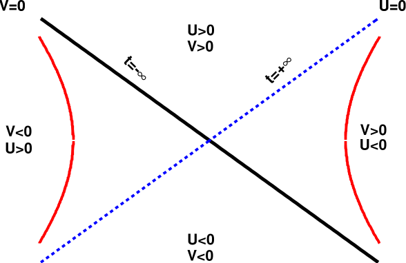
Figure 3: Kruskal diagram for the AdS black hole. The coordinates $(t,r)$ span the right quadrant. The thick hyperbolas on the sides of the two quadrants are the boundaries at $r=\infty$. The boundary in the right and left quadrants correspond to the “1” and “2” axes of the thermal field theory respectively. The static quark corresponds to a string which spans the full Kruskal plane. At finite velocity, the asymptotic solution Eq. (38) is discontinuous at $t=-\infty$ or $V=0$.

As the electric field is turned on in the gauge theory, the quark accelerates and slowly approaches the stationary velocity distribution. In the gravity dual this corresponds to slowly turning on a $U(1)$ electric field in the boundary brane and waiting for the string to reach the asymptotic form given by Eq. (38). We re-write this solution in Kruskal coordinates as

$$x_{3}=\frac{v}{2}\log(V)+v\,\arctan(z)\qquad\mbox{for $V>0$}\,.$$ (42)

Examining this solution we see a logarithmic divergence for $V\rightarrow 0$, i.e. in the distant past, $t\rightarrow-\infty$. This discontinuity in the distant past reflects the fact that the asymptotic solution Eq. (42) is not a solution as the electric field was turned on slowly. At $t\rightarrow-\infty$ it is reasonable expect that this solution slowly deforms into the static solution described above and covers the full Kruskal plane.

Therefore, we will demand analyticity across the $V=0$ line while extending $V$ through the lower half plane to negative real argument  . Through this process $x_{3}$ becomes imaginary

$$x_{3}=\frac{v}{2}\log(\left|V\right|)+v\,\arctan(z)-iv\underbrace{\pi/2}_{\beta/2}\,.$$ (43)

This imaginary value for the coordinate $x_{3}$ is appropriate. The left quadrant of the Kruskal plane is associated with the “2” branch of the field theory with $\sigma=i\beta/2$, or $i\pi/2$ for our rescaled units. Since the operators on the real axis are evaluated at the space time point $(t,x_{3})=(t,vt)$, when time is extended in the imaginary time direction we expect that the operators should be evaluated at

$$(t,vt)\rightarrow(t-i\beta/2,vt-iv\beta/2)\,.$$ (44)

Thus the analytic extension of the string solution into the lower half $V$ plane maps to the appropriate $x_{3}$ coordinate.

In what follows we will take this string solution as the gravity dual of the heavy quark (or Wilson line) propagating along the Schwinger-Keyldish contour shown in Fig. 1 with the second axis displaced by $i\beta/2$. We will make the correspondence between the “1” and “2” axes of the contour and the endpoints of the string on the right and left boundaries of AdS. When studying fluctuations of this semi-classical string solution, we will bear in mind this discussion of the past infinity and demand analyticity across the $V=0$ line.

III.3 Fluctuations and World Sheet Black Hole

Having constructed the string solution corresponding to a heavy quark propagating along the Schwinger Keldysh contour, we will proceed to fluctuate the shape of the string solutions in the transverse directions and solve for the fluctuations. Once the classical solution is determined in the Kruskal plane we follow the general philosophy of the AdS/CFT correspondence and equate the classical action of the source to the generating functional

$$\frac{1}{e^{iS_{NG}[0,0]}}e^{iS_{NG}[\delta y_{1},\delta y_{2}]}=\frac{1}{\left\langle{\rm tr}\,\rho^{o}\,W[0,0]\right\rangle_{A}}\,\left\langle{\rm tr}\,\rho^{o}\,W[\delta y_{1},\delta y_{2}]\right\rangle_{A}\,.$$ (45)

However in order to find the classical solution, boundary conditions are needed. The appropriate boundary conditions for $G_{11}$ and $G_{22}$ etc. are not obvious.

The appropriate boundary conditions are greatly clarified by a change of coordinates which transforms the original induced metric to a diagonal metric which turns out to be equivalent to a world sheet black hole. Using the original coordinates $(\tau,\sigma)=(t,z)$ the induced metric is

$$h_{tt} = -\frac{R^{2}}{z^{2}}\left(\frac{1}{\gamma^{2}}-z^{4}\right)\,,$$ (46)

$$h_{zz} = \frac{R^{2}}{z^{2}}\frac{1}{f^{2}}\left(1-\frac{z^{4}}{\gamma^{2}}\right)\,,$$ (47)

$$h_{tz} = -\frac{R^{2}}{z^{2}}\frac{1}{f}v^{2}z^{2}\,.$$ (48)

This non-diagonal world sheet metric can be diagonalized by the following change of coordinates

$$\hat{t} = \frac{1}{\sqrt{\gamma}}\left(t+\frac{1}{2}\arctan(z)-\frac{1}{2}\sqrt{\gamma}\arctan(\sqrt{\gamma}z)-\frac{1}{2}\rm{arctanh}(z)+\frac{1}{2}\sqrt{\gamma}\rm{artanh}(\sqrt{\gamma}z)\right)\,,$$ (49)

$$\hat{z} = \sqrt{\gamma}z\,.$$ (50)

and the metric takes the form

$$h_{{\hat{t}}{\hat{t}}} = -\frac{R^{2}}{{\hat{z}}^{2}}f({\hat{z}})\,,$$ (51)

$$h_{{\hat{z}}{\hat{z}}} = \frac{R^{2}}{{\hat{z}}^{2}}\frac{1}{f({\hat{z}})}\,,$$ (52)

$$h_{{\hat{t}}{\hat{z}}} = 0\,,$$ (53)

with $f({\hat{z}})=1-{\hat{z}}^{4}$. Thus the world sheet metric is in fact a black hole with the horizon at $z^{2}=1/\gamma$ or $\hat{z}=1$ . As usual, the horizon is a coordinate singularity and is a consequence the coordinate transformation in Eq. (49). In this coordinate system, the induced metric for the moving string with “hat” variables equals the induced metric of the static string with “un-hatted” variables.

Next we show how different regions of the world-sheet black hole map into space time. First we define the analogs of Kruskal variables for hatted variables $\hat{\nu}_{-},\hat{\nu}_{+},\hat{V},\hat{U},\hat{z}_{*},\dots$. (For instance $\hat{z}_{*}=(\tan^{-}1({\hat{z}})+\tanh^{-}1({\hat{z}}))/2$ ). Taking $\hat{V}$ positive, we have the following relation between the world-sheet and space-time Kruskal variables

$$\hat{z} = \sqrt{\gamma}z\,,$$ (54)

$$\hat{V^{\prime}} = \left(V^{\prime}\right)^{1/\sqrt{\gamma}}\,,$$ (55)

$$\hat{X^{\prime}}=\frac{1-\hat{z}}{1+\hat{z}} X^{\prime}=\frac{1-{z}}{1+{z}}\,.$$ (56)

From the form of this map we see the upper half of the world sheet Kruskal plane $(\hat{U},\hat{V})$ gets mapped into the upper half Kruskal plane of space-time $V>0$. The structure is illustrated in Fig. 4.

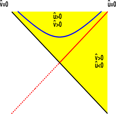
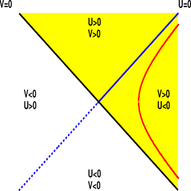
Figure 4: (a) The world sheet black hole. (b) The Schwarzschild black hole in space time. The future event horizon of the world sheet and its corresponding image $z=1/\sqrt{\gamma}$ are indicated by the solid red line. Similarly the solid blue line maps to the future event horizon of the space time black hole. The shaded region of the world sheet black hole maps into the shaded region of space-time region of the Schwarzschild geometry. Similarly there is a separate string solution in the $V<0$ half of the $(U,V)$ plane which maps to the $\hat{V}<0$ half of the $(\hat{U},\hat{V})$ plane. The two solutions are joined at past infinity ($V=0$) by demanding analyticity in the lower complex $V$ plane, i.e. that only positive energy solutions emerge from past infinity.

As $V$ becomes negative $\hat{V}$ becomes imaginary. This is because the solution given in Eq. (38) is not valid at past infinity. In the lower half $(V<0)$ of the Kruskal plane we can find a separate string solution which maps the lower half ($\hat{V}<0$) of the world sheet Kruskal plane. At past infinity, before the electric field was turned on, the quark is at rest, and the two string solution are joined. We will therefore connect the solutions in the upper half and lower half Kruskal planes by demanding analyticity across the $V=0$ line, extending $V$ through the lower half complex $V$ plane. This extension through the lower complex $V$ plane is consistent with the Herzog-Son construction Herzog:2002pc and physically says that only positive energy solutions emerge from past infinity. Again by analogy with the Herzog-Son construction, we will extend through the upper complex $\hat{U}$ plane. Physically this says that only negative energy solutions emerge from the future event horizon of the world sheet black hole.

Having clarified the analytic structure of the world sheet black hole and determined the appropriate boundary conditions, we next analyze small fluctuations. The equation of motion for small transverse fluctuations can be found easily in “hatted” coordinate system. Introducing

$${\hat{y}}=\sqrt{\gamma}y\,,$$ (57)

the action for small fluctuation is the same as for the static string Casalderrey-Solana:2006rq

$$S_{NG}=\frac{R^{2}}{2\pi\alpha^{\prime}}\int\frac{d{\hat{t}}\,d{\hat{u}}}{2{\hat{u}}^{3/2}}\left[1-\frac{1}{2}\left(\frac{\dot{{\hat{y}}}^{2}}{f({\hat{u}})}-4f({\hat{u}}){\hat{u}}\left({\hat{y}}^{\prime}\right)^{2}\right)\right]\,.$$ (58)

We define,

$${\hat{y}}({\hat{t}},{\hat{u}})=\int e^{-i{\hat{\omega}}{\hat{t}}}\,{\hat{y}}({\hat{\omega}})\,{\hat{Y}}({\hat{\omega}},{\hat{u}})\,\frac{d{\hat{\omega}}}{2\pi}\,.$$ (59)

where we choose to normalize ${\hat{Y}}_{\hat{\omega}}({\hat{u}}=0)=1$, i.e. ${\hat{y}}(\omega)$ is the value of the fluctuation at the boundary.

The Euler-Lagrange equation for the small string fluctuations are

$$\partial_{{\hat{u}}}^{2}{\hat{Y}}_{\hat{\omega}}-\frac{(2+6{\hat{u}}^{2})}{4{\hat{u}}f}\partial_{\hat{u}}{\hat{Y}}_{\hat{\omega}}+\frac{{\hat{\omega}}^{2}}{4{\hat{u}}f^{2}}{\hat{Y}}_{\hat{\omega}}=0\,.$$ (60)

This equation is solved by

$${\hat{Y}}({\hat{\omega}},u)=\left(1-{\hat{u}}\right)^{-i{\hat{\omega}}/4}{\hat{F}}({\hat{\omega}},{\hat{u}})$$ (61)

where ${\hat{F}}({\hat{u}})$ is a regular function of ${\hat{u}}>0$ . $(1-{\hat{u}})^{-i{\hat{\omega}}/4}$ is in-falling in the world-sheet horizon ${\hat{u}}=1$. The complex conjugate of this expression is also a solution of the differential equation and is outgoing at the horizon.

Let us now extend these solutions into the full Kruskal plane. It is useful to express the solution in terms of the world sheet Kruskal coordinates. Close to $\hat{z}=1$ the in-falling solution and out-going solutions behave as

$$e^{-i{\hat{\omega}}{\hat{t}}}{\hat{Y}}({\hat{\omega}},{\hat{u}}) \sim e^{-i{\hat{\omega}}/2\ln(\hat{V})}\qquad\mbox{in-falling}$$ (62)

$$e^{-i{\hat{\omega}}{\hat{t}}}{\hat{Y}}^{*}({\hat{\omega}},{\hat{u}}) \sim e^{i{\hat{\omega}}/2\ln(-\hat{U})}\qquad\mbox{out-going}$$ (63)

As mentioned before, the coordinate $\hat{V}$ does not cross zero in this $z=\sqrt{u}=1/\sqrt{\gamma}$. However, $\hat{U}$ does and we should be careful when defining the branch cut for the logarithm. In analogy with the Herzog-Son prescription, we will impose that the solution should be analytic in the upper half of the complex ${\hat{U}}$ plane. Since ${\hat{U}}$ is negative in this quadrant, the prescription means that

$$e^{-i{\hat{\omega}}{\hat{t}}}{\hat{Y}}^{*}({\hat{\omega}},{\hat{u}})\sim e^{\pi{\hat{\omega}}/2}e^{i{\hat{\omega}}/2\ln(\hat{U})}\,.$$ (64)

Thus, when the fluctuation crosses the world-sheet event horizon in the right quadrant it picks a factor $\exp\{\pi{\hat{\omega}}/2\}$. Due to the different relation between ${\hat{U}}$ and the local $({\hat{t}},{\hat{z}})$ coordinates, in the left quadrant the solution behaves as

$$e^{-i{\hat{\omega}}{\hat{t}}}{\hat{Y}}^{*}({\hat{\omega}},{\hat{u}})\sim e^{i{\hat{\omega}}/2\ln(\hat{U})}\,.$$ (65)

Thus, after passing the world sheet horizon, keeping the same analyticity properties in ${\hat{U}}$, the solution picks a factor $\exp\{-\pi{\hat{\omega}}/2\}$ in the L-quadrant.

We now address how the matching of left and right quadrant is performed. Using the change of coordinates Eq. (49) we obtain (for ${\hat{u}}<1$)

$$e^{-i{\hat{\omega}}{\hat{t}}}{\hat{Y}}({\hat{\omega}},{\hat{u}}) = e^{-i\omega t}(1-u)^{-i\omega/4}F_{i}(\omega,u)\,,$$ (66)

$$e^{-i{\hat{\omega}}{\hat{t}}}{\hat{Y}}^{*}({\hat{\omega}},{\hat{u}}) = e^{-i\omega t}(\frac{1}{\gamma}-u)^{i{\hat{\omega}}/2}(1-u)^{-i\omega/4}F_{o}(\omega,u)\,,$$ (67)

where we have defined $\omega={\hat{\omega}}/\sqrt{\gamma}$ and $F_{i}(\omega,u)$, $F_{o}(\omega,u)$ are two regular solutions in u. The pole at $u=1/\sqrt{\gamma}$ in the outgoing solution is a consequence of crossing the ${\hat{U}}=0$ line. Note that this pole does not appear in the in-falling solution, since we do not cross the ${\hat{V}}=0$ line. From this point of view, the previous prescription for the analytic properties of the solution in the ${\hat{U}}$ coordinate translates into the prescription for going around the pole in $u=1/\sqrt{\gamma}$. Taking this prescription into account, in the R quadrant the two solutions close to the horizon behave as

$$e^{-i{\hat{\omega}}{\hat{t}}}{\hat{Y}}({\hat{\omega}},{\hat{u}}) \sim e^{-i\omega/2\ln(V)}\,,$$ (68)

$$e^{-i{\hat{\omega}}{\hat{t}}}{\hat{Y}}^{*}({\hat{\omega}},{\hat{u}}) \sim e^{\pi{\hat{\omega}}/2}e^{-i\omega/2\ln(V)}\,.$$ (69)

Note that from the point of view of the AdS black-hole both solutions are in-falling. The exponential factor in the outgoing solution is a consequence of the prescription to cross the pole at ${\hat{u}}=1$. In the same way, the fluctuations in the L-quadrant behave as

$$e^{-i{\hat{\omega}}{\hat{t}}}{\hat{Y}}({\hat{\omega}},{\hat{u}}) \sim e^{-i\omega/2\ln(-V)}\,,$$ (70)

$$e^{-i{\hat{\omega}}{\hat{t}}}{\hat{Y}}^{*}({\hat{\omega}},{\hat{u}}) \sim e^{-\pi{\hat{\omega}}/2}e^{-i\omega/2\ln(-V)}\,.$$ (71)

With these four expression we find four different solutions defined in both quadrants of the (AdS) Kruskal plane

$${\hat{y}}_{R,i}=\left\{\begin{array}[]{ll}e^{-i{\hat{\omega}}{\hat{t}}}{\hat{Y}}({\hat{\omega}},{\hat{u}})&\mbox{in R}\\ 0&\mbox{in L}\end{array}\right.\;\;\;\;\;\;\;\;\;\;{\hat{y}}_{L,i}=\left\{\begin{array}[]{ll}0&\mbox{in R}\\ e^{-i{\hat{\omega}}{\hat{t}}}{\hat{Y}}({\hat{\omega}},{\hat{u}})&\mbox{in L}\end{array}\right.\ ,$$ (72)

$${\hat{y}}_{R,o}=\left\{\begin{array}[]{ll}e^{-i{\hat{\omega}}{\hat{t}}}{\hat{Y}}^{*}({\hat{\omega}},{\hat{u}})&\mbox{in R}\\ 0&\mbox{in L}\end{array}\right.\;\;\;\;\;\;\;\;\;\;{\hat{y}}_{L,o}=\left\{\begin{array}[]{ll}0&\mbox{in R}\\ e^{-i{\hat{\omega}}{\hat{t}}}{\hat{Y}}^{*}({\hat{\omega}},{\hat{u}})&\mbox{in L}\end{array}\right.\,.$$ (73)

Following the Herzog-Son prescription Herzog:2002pc , we look for linear combinations of these expressions that, close to the horizon, are analytic in the lower half of the complex $V$ plane. With this criterium only two linear combinations can be found:

$${\hat{y}}_{o}={\hat{y}}_{R,o}+\alpha_{o}{\hat{y}}_{L,o}\,,$$ (74)

$${\hat{y}}_{i}={\hat{y}}_{R,i}+\alpha_{i}{\hat{u}}_{L,i}\,.$$ (75)

From the close to horizon behaviors of the solutions Eq. (68), Eq. (69), Eq. (70), Eq. (71), the analyticity properties demand

$$\alpha_{o} = e^{+\pi{\hat{\omega}}}e^{-\pi\omega/2}\,,$$ (76)

$$\alpha_{i} = e^{-\pi\omega/2}\,.$$ (77)

These two solutions are used as a basis for the linearized string fluctuations defined over the full (AdS) Kruskal plane

$${\hat{y}}=\int\frac{d{\hat{\omega}}}{2\pi}\left(a(\omega){\hat{y}}_{o}(\omega)+b(\omega){\hat{y}}_{i}(\omega)\right)\,.$$ (78)

This prescription recovers the results of Herzog and Son Herzog:2002pc when $\gamma=1$. To see this one has to realize that when $\gamma=1$, since these solutions are only defined for $u<1$ we do not cross the pole and, thus, the exponential prefactors in ${\hat{y}}_{\{L,R\}o}$ do not appear.

The coefficients $a({\hat{\omega}}),b({\hat{\omega}})$ can be determined by the boundary values of the solutions. Thus, if we have

$${\hat{y}}({\hat{t}},{\hat{u}}=0)\big{|}_{R} = \int\frac{d{\hat{\omega}}}{2\pi}e^{-i{\hat{\omega}}{\hat{t}}}{\hat{y}}_{1}({\hat{\omega}})\,,$$ (79)

$${\hat{y}}({\hat{t}},{\hat{u}}=0)\big{|}_{L} = \int\frac{d{\hat{\omega}}}{2\pi}e^{-i{\hat{\omega}}{\hat{t}}}{\hat{y}}_{2}({\hat{\omega}})\,,$$ (80)

we obtain

$$a(\omega) = \frac{1}{e^{\pi{\hat{\omega}}}-1}\left(-{\hat{y}}_{1}({\hat{\omega}})+{\hat{y}}_{2}({\hat{\omega}})e^{\pi\omega/2}\right)\,,$$ (81)

$$b(\omega) = \frac{1}{e^{\pi{\hat{\omega}}}-1}\left(e^{\pi{\hat{\omega}}}{\hat{y}}_{1}({\hat{\omega}})-e^{\pi\omega/2}{\hat{y}}_{2}({\hat{\omega}})\right)\,.$$ (82)

We can now compute the boundary action in terms of the string solutions. In $(\hat{t},\hat{u})$ coordinates

$$S_{B}=\frac{R^{2}}{2\pi\alpha}\left[\int_{R}\frac{d\hat{\omega}}{2\pi}\frac{1}{\hat{u}^{1/2}}{\hat{y}}(-\hat{\omega},\hat{u})\partial_{\hat{u}}{\hat{y}}(\hat{\omega},\hat{u})-\int_{L}\frac{d\hat{\omega}}{2\pi}\frac{1}{\hat{u}^{1/2}}{\hat{y}}(-\hat{\omega},\hat{u})\partial_{\hat{u}}{\hat{y}}(\hat{\omega},\hat{u})\right]\,.$$ (83)

Using Eq. 81 this action can be expressed as

$$S_{B} = \frac{R^{2}}{2\pi\alpha}\sqrt{\gamma}\int\frac{d\omega}{2\pi}\Big{[}$$

$$y_{1}(-\omega)y_{1}(\omega)\left(({\hat{n}}+1)\frac{1}{\hat{u}^{1/2}}{\hat{Y}}^{*}(-\hat{\omega},\hat{u})\partial_{\hat{u}}{\hat{Y}}(\hat{\omega},\hat{u})-{\hat{n}}\frac{1}{\hat{u}^{1/2}}{\hat{Y}}(-\hat{\omega},\hat{u})\partial_{\hat{u}}{\hat{Y}}^{*}(\hat{\omega},\hat{u})\right)+$$

$$y_{1}(-\omega)y_{2}(\omega)e^{\pi\omega/2}{\hat{n}}\left(-\frac{1}{\hat{u}^{1/2}}{\hat{Y}}^{*}(-\hat{\omega},\hat{u})\partial_{\hat{u}}{\hat{Y}}(\hat{\omega},\hat{u})+\frac{1}{\hat{u}^{1/2}}{\hat{Y}}(-\hat{\omega},\hat{u})\partial_{\hat{u}}{\hat{Y}}^{*}(\hat{\omega},\hat{u})\right)+$$

$$y_{2}(-\omega)y_{1}(\omega)e^{-\pi\omega/2}(1+{\hat{n}})\left(-\frac{1}{\hat{u}^{1/2}}{\hat{Y}}^{*}(-\hat{\omega},\hat{u})\partial_{\hat{u}}{\hat{Y}}(\hat{\omega},\hat{u})+\frac{1}{\hat{u}^{1/2}}{\hat{Y}}(-\hat{\omega},\hat{u})\partial_{\hat{u}}{\hat{Y}}^{*}(\hat{\omega},\hat{u})\right)+$$

$$y_{2}(-\omega)y_{2}(\omega)\left({\hat{n}}\frac{1}{\hat{u}^{1/2}}{\hat{Y}}^{*}(-\hat{\omega},\hat{u})\partial_{\hat{u}}{\hat{Y}}(\hat{\omega},\hat{u})-({\hat{n}}+1)\frac{1}{\hat{u}^{1/2}}{\hat{Y}}(-\hat{\omega},\hat{u})\partial_{\hat{u}}{\hat{Y}}^{*}(\hat{\omega},\hat{u})\right)\Big{]}\,\,,$$

where ${\hat{n}}=1/(\exp\{\pi\hat{\omega}\}-1)$ and we have used the fact that ${\hat{y}}_{1,2}({\hat{\omega}})=y_{1,2}(\omega)$. From this expression we can read off immediately the different correlators by taking derivatives with respect to the boundary values. In particular

$$\lim_{\omega\longrightarrow 0}iG_{12}(\omega) = \lim_{\omega\longrightarrow 0}iG_{21}(\omega)=\lim_{\omega\longrightarrow 0}\frac{1}{2}\left(iG_{11}(\omega)+iG_{22}(\omega)\right)\,,$$ (85)

$$= \lim_{\omega\longrightarrow 0}\frac{R^{2}}{\pi\alpha}\frac{2}{\pi{\hat{\omega}}}\sqrt{\gamma}\,{\rm Im}\left\{\frac{1}{{\hat{u}}^{1/2}}{\hat{Y}}^{*}(-\hat{\omega},\hat{u})\partial_{\hat{u}}{\hat{Y}}(\hat{\omega},\hat{u})\right\}$$

Since the action for the fluctuation Eq. (58) is formally the same as that of the static string, we obtain the same result for the transverse momentum transferred as in the static case (up to an overall factor of $\sqrt{\gamma}$). After restoring physical units and using the result of Casalderrey-Solana:2006rq and Eq. (33)

$$\kappa_{T}=\sqrt{\gamma\lambda}T^{3}\pi\,.$$ (86)

IV Conclusions

In this paper we have studied the medium modifications of a heavy quark that propagates in a strongly coupled plasma at finite velocity $v$. Starting from the density matrix of the quark, we have expressed the transverse momentum broadening of the probe as a Wilson loop running along the $x=v\,t$ line, with a transverse separation, $\Delta x$. This Wilson loop is similar to that considered in Refs. Liu:2006he ; Liu:2006ug but approaches the lightcone from below. The second derivative of this Wilson loop with respect to the transverse separation $\Delta x$ yields $\kappa_{T}$ – the mean squared transverse momentum transfer per unit time acquired by the probe in its propagation through the medium. We have stressed that the appropriate Wilson loop has a time ordered line and an anti-time ordered line. These two pieces can be understood as the quark’s amplitude and complex conjugate amplitude respectively. Due to this specific time ordering, we have introduced the type “1” and type “2” fields of Schwinger-Keyldish formalism Keldysh:1964ud ; Schwinger:1960qe . The sources for these type “1” and type “2” fields correspond o the boundary values of SUGRA fields in right and left quadrants of the Kruskal plane.

To construct the gravity dual of this (“1”,“2”) Wilson loop we have extended the moving quark string solution found in Refs. Yaffe ; Gubser:2006bz to the left Kruskal quadrant. The string world sheet is disconnected along the $V=0$ line because the $V=0$ line represents the distant past. In the distant past the moving quark string is not a solution to the equations of motion because the electric field used to accelerate the quark is being slowly turned on. At past infinity the two disconnected solutions are joined by demanding analyticity in the lower half plane $V$ as required by the correspondence between AdS black holes and the real time thermal field theory.

Subsequently we have computed $\kappa_{T}$ by fluctuating the transverse position of the string endpoint and solving for the standing waves. To determine the correct boundary conditions, we first noticed that the induced metric of the string worldsheet is that of a black hole. The event horizon of this world sheet black hole maps to the line $r=r_{o}\sqrt{\gamma}$, with $r_{o}$ the event horizon of the AdS black hole. Then, borrowing from the work of Herzog and Son Herzog:2002pc , we have analytically continued the fluctuations through both the world-sheet and AdS horizons. This analytic extension amounts to specifying the boundary conditions on the physically correct solutions in the full Kruskal plane. From the solution in the full Kruskal plane we obtain

$$\kappa_{T}=\sqrt{\gamma\lambda}T^{3}\pi\,,$$ (87)

which diverges in the $v\rightarrow 1$ limit.

Finally we wish to compare $\kappa_{T}$ (the mean squared transverse momentum transfer to a heavy quark per unit time) to $\hat{q}$. Up to a factor of two, the definition of $\kappa_{T}$ given here is often ascribed to $\hat{q}$, at least if the qualifier “heavy” is removed from heavy quark. However, the value $2\kappa_{T}$ differs from the value of the jet quenching parameter found by Liu, Rajagopal and Wiedemann (LRW) Liu:2006he ; Liu:2006ug

$$\hat{q}_{LRW}=\frac{\pi^{3/2}\Gamma(\frac{3}{4})}{2\Gamma(\frac{5}{4})}\sqrt{\lambda}T^{3}\,.$$ (88)

LRW use the dipole formula as a definition of $\hat{q}$ and compute a strictly lightlike Wilson loop. This Wilson loop corresponds into a space-like surface. In this computation special care has to be taken in approaching the limits $M\rightarrow\infty$ and $v\rightarrow 1$. Regardless of the concern expressed by some authors about this computation Yaffe ; Chernicoff:2006hi ; Argyres:2006yz (most of which have been addressed in Liu:2006he ), we do not completely understand the source of this discrepancy. The difference between the two results may lie in the fact that the Wilson line in Ref. Liu:2006he ; Liu:2006ug is strictly light like.

Certainly the calculation described here is limited to the regime

$$\gamma<\left(\frac{M}{\sqrt{\lambda}T}\right)^{2}\,.$$ (89)

To see this we recall that the quark moving with velocity $v$ was constructed by slowly turning on an electric field and accelerating the quark to its terminal velocity Yaffe . The equation of motion of the quark is

$$\frac{dp}{dt}=-\eta p+E\,,$$ (90)

with $\eta\sim\sqrt{\lambda}T^{2}/M$. The electric field can be increased until its critical value, which can be computed from the Born-Infeld action for the probe brane in the AdS geometry,

$$S_{BI}\sim\sqrt{1-\left(2\pi\alpha^{\prime}E\frac{R^{2}}{r^{2}}\right)^{2}}\,.$$ (91)

The critical value for the electric field is then

$$E<\frac{M^{2}}{\sqrt{\lambda}}\,.$$ (92)

Equating $E\sim\eta p$ we obtain the bound written above, Eq. (89). Nevertheless by taking the mass to infinity we may approach the lightlike Wilson line from below.

In summary, the discrepancy may have its origin in the derivation of the dipole formula or in the relation between radiative energy loss and the squared momentum transfer. Both of these analyses are derived in perturbation theory. A careful analysis of the approximations needed to derive these results may resolve the discrepancy and lead to a deeper understanding of radiation in a strongly coupled field theory.

Note Added. During the completion of this work a preprint by S. Gubser, hep-th/0612143, appeared and revealed the properties of the world sheet black hole. We gratefully acknowledge illuminating discussions over the past weeks with Professor Gubser, who pointed out (amongst other things) an algebraic error in our draft which had led to a $\kappa_{T}$ independent of the quark velocity. Even after correcting this error this manuscript did not agree with the first version of hep-th/0612143. The differences have since been resolved.

Acknowledgments. J.C thanks J. L. Albacete, N. Armesto, V. Koch, C. Salgado, X. N. Wang, U. A. Wiedemann for useful discussions about the computation of radiative losses and H. Liu about the computation of the light-like Wilson Loops. This work was supported by the Director, Office of Science, Office of High Energy and Nuclear Physics, Division of Nuclear Physics, and by the Office of Basic Energy Sciences, Division of Nuclear Sciences, of the U.S. Department of Energy under Contract No. DE-AC03-76SF00098.

References

• (1) K. Adcox et al. [PHENIX Collaboration], Phys. Rev. Lett.  88, 022301 (2002) [arXiv:nucl-ex/0109003].
• (2) C. Adler et al. [STAR Collaboration], Phys. Rev. Lett.  89, 202301 (2002) [arXiv:nucl-ex/0206011].
• (3) X.  N.  Wang, M.  Gyulassy and M.  Plumer, Phys. Rev. D 51 (1995) 3436
M. Gyulassy, I. Vitev, X. N. Wang and B. W. Zhang, arXiv:nucl-th/0302077.
• (4) A. Kovner and U. A. Wiedemann, arXiv:hep-ph/0304151.
• (5) R.  Baier, Y.  L. Dokshitzer,A.  H.  Mueller,S.  Peigne and D. Schiff, Nucl. Phys. B 483 (1997) 291
R.  Baier , Y. L.  Dokshitzer, A.  H.  Mueller and D.  Schiff, JHEP 0109 (2001) 033
• (6) K. J. Eskola, H. Honkanen, C. A. Salgado and U. A. Wiedemann, Nucl. Phys. A 747, 511 (2005) [arXiv:hep-ph/0406319].
• (7) A. Dainese, C. Loizides and G. Paic, Eur. Phys. J. C 38, 461 (2005) [arXiv:hep-ph/0406201].
• (8) S. S. Adler et al. [PHENIX Collaboration], Phys. Rev. Lett.  91, 182301 (2003) [arXiv:nucl-ex/0305013].
• (9) K. H. Ackermann et al. [STAR Collaboration], Phys. Rev. Lett.  86, 402 (2001) [arXiv:nucl-ex/0009011].
• (10) P. F. Kolb, U. W. Heinz, P. Huovinen, K. J. Eskola and K. Tuominen, Nucl. Phys. A 696, 197 (2001) [arXiv:hep-ph/0103234].
• (11) D. Teaney, J. Lauret and E. V. Shuryak, arXiv:nucl-th/0110037.
• (12) J. M. Maldacena, Adv. Theor. Math. Phys.  2, 231 (1998) [Int. J. Theor. Phys.  38, 1113 (1999)] [arXiv:hep-th/9711200].
• (13) Phys. Lett. B 428, 105 (1998) [arXiv:hep-th/9802109].
• (14) E. Witten, Adv. Theor. Math. Phys.  2, 253 (1998) [arXiv:hep-th/9802150].
• (15) G. Policastro, D. T. Son and A. O. Starinets, Phys. Rev. Lett.  87, 081601 (2001) [arXiv:hep-th/0104066].
• (16) C. P. Herzog, A. Karch, P. Kovtun, C. Kozcaz and L. G. Yaffe, JHEP 0607, 013 (2006) [arXiv:hep-th/0605158].
• (17) S. S. Gubser, arXiv:hep-th/0605182.
• (18) J. Casalderrey-Solana and D. Teaney, Phys. Rev. D 74, 085012 (2006) [arXiv:hep-ph/0605199].
• (19) C. P. Herzog, JHEP 0609, 032 (2006) [arXiv:hep-th/0605191].
• (20) E. Caceres and A. Guijosa, JHEP 0611, 077 (2006) [arXiv:hep-th/0605235].
• (21) S. J. Sin and I. Zahed, arXiv:hep-ph/0606049.
• (22) E. Caceres and A. Guijosa, JHEP 0612, 068 (2006) [arXiv:hep-th/0606134].
• (23) M. Chernicoff and A. Guijosa, arXiv:hep-th/0611155.
• (24) P. Talavera, arXiv:hep-th/0610179.
• (25) H. Liu, K. Rajagopal and U. A. Wiedemann, arXiv:hep-ph/0607062.
• (26) K. Peeters, J. Sonnenschein and M. Zamaklar, Phys. Rev. D 74, 106008 (2006) [arXiv:hep-th/0606195].
• (27) M. Chernicoff, J. A. Garcia and A. Guijosa, JHEP 0609, 068 (2006) [arXiv:hep-th/0607089].
• (28) J. J. Friess, S. S. Gubser, G. Michalogiorgakis and S. S. Pufu, arXiv:hep-th/0609137.
• (29) P. C. Argyres, M. Edalati and J. F. Vazquez-Poritz, arXiv:hep-th/0608118.
• (30) S. D. Avramis, K. Sfetsos and D. Zoakos, arXiv:hep-th/0609079.
• (31) J. J. Friess, S. S. Gubser, G. Michalogiorgakis and S. S. Pufu, arXiv:hep-th/0607022.
• (32) J. J. Friess, S. S. Gubser and G. Michalogiorgakis, JHEP 0609, 072 (2006) [arXiv:hep-th/0605292].
• (33) E. Shuryak, S. J. Sin and I. Zahed, arXiv:hep-th/0511199.
• (34) S. Lin and E. Shuryak, arXiv:hep-ph/0610168.
• (35) R. A. Janik and R. Peschanski, Phys. Rev. D 74, 046007 (2006) [arXiv:hep-th/0606149].
• (36) J. J. Friess, S. S. Gubser, G. Michalogiorgakis and S. S. Pufu, arXiv:hep-th/0611005.
• (37) S. J. Sin, S. Nakamura and S. P. Kim, arXiv:hep-th/0610113.
• (38) B. G. Zakharov, JETP Lett.  65, 615 (1997) [arXiv:hep-ph/9704255].
• (39) A. Buchel, Phys. Rev. D 74, 046006 (2006) [arXiv:hep-th/0605178].
• (40) J. F. Vazquez-Poritz, arXiv:hep-th/0605296.
• (41) S. D. Avramis and K. Sfetsos, arXiv:hep-th/0606190.
• (42) N. Armesto, J. D. Edelstein and J. Mas, JHEP 0609, 039 (2006) [arXiv:hep-ph/0606245].
• (43) R. Baier, Y. L. Dokshitzer, A. H. Mueller, S. Peigne and D. Schiff, Nucl. Phys. B 484, 265 (1997) [arXiv:hep-ph/9608322].
• (44) H. Liu, K. Rajagopal and U. A. Wiedemann, Phys. Rev. Lett.  97, 182301 (2006) [arXiv:hep-ph/0605178].
• (45) H. Liu, K. Rajagopal and U. A. Wiedemann, arXiv:hep-ph/0612168.
• (46) Leo P. Kadanoff and Gordon Baym, Quantum statistical mechanics, Cambridge, Massachuessets: Perseus Books (1989).
• (47) J. P. Blaizot and E. Iancu, Phys. Rept.  359, 355 (2002) [arXiv:hep-ph/0101103].
• (48) S. Weinberg, The Quantum Theory of Fields, Vol. II., New York, New York: Cambridge University Press (2002).
• (49) E. Braaten and Y. Jia, Phys. Rev. D 63, 096009 (2001) [arXiv:hep-ph/0003135].
• (50) O. Aharony, S. S. Gubser, J. M. Maldacena, H. Ooguri and Y. Oz, Phys. Rept.  323, 183 (2000) [arXiv:hep-th/9905111].
• (51) S. S. Gubser, arXiv:hep-th/0612143.
• (52) C. P. Herzog and D. T. Son, JHEP 0303, 046 (2003) [arXiv:hep-th/0212072].
• (53) L. V. Keldysh, Zh. Eksp. Teor. Fiz.  47, 1515 (1964) [Sov. Phys. JETP 20, 1018 (1965)].
• (54) J. S. Schwinger, J. Math. Phys.  2, 407 (1961).
• (55) P. C. Argyres, M. Edalati and J. F. Vazquez-Poritz, arXiv:hep-th/0612157.