Typicality versus thermality: An analytic distinction

In systems with a large degeneracy of states such as black holes, one expects that the average value of probe correlation functions will be well approximated by the thermal ensemble. To understand how correlation functions in individual microstates differ from the canonical ensemble average and from each other, we study the variances in correlators. Using general statistical considerations, we show that the variance between microstates will be exponentially suppressed in the entropy. However, by exploiting the analytic properties of correlation functions we argue that these variances are amplified in imaginary time, thereby distinguishing pure states from the thermal density matrix. We demonstrate our general results in specific examples and argue that our results apply to the microstates of black holes.

1 Introduction

Our usual understanding of effective field theory suggests that the well-known classical geometry of a black hole spacetime is valid past the horizon through to a Planck distance away from the singularity. Recently, however, it has been proposed that the microstates of black holes form a sort of spacetime foam that extends throughout the interior of the horizon [2]. Such a magnification of the characteristic length scale of quantum gravity recalls macroscopic manifestations of quantum mechanics such as Bose condensation that appear due to the statistical interactions of many microscopic constituents.

The proposed non-singular, horizon-free, spacetime foam microstates have only been constructed for certain extremal black holes in string theory. In the classical limit, they are characterized by a large topologically complex region within which the characteristic scale is microscopic. However, the foam itself extends out to macroscopic distances, behaving in some cases like an incompressible fluid. These solutions should be understood as a classical moduli space of candidate microstates which must be quantized. A key question is whether a semiclassical observer probing such quantized microstates makes measurements that are different from those expected from the usual black hole spacetimes. If they are not, the usual classical geometries are the correct effective description of a black hole for a semiclassical observer, even though observers with more precise tools or greater patience might observe a horizon- and singularity-free universe [10, 12, 14].

These questions are most efficiently studied when the black holes and their microstates are asymptotic to AdS spacetime. In this case, the dual field theory can be used to enumerate the microstates and quantize them. We can then ask whether the correlation functions of probe operators can distinguish the microstates from each other or tell them apart from a mixed state. This involves computing the variance of correlation functions over a suitable ensemble of pure microstates with given macroscopic quantum numbers. In Sec. 2 we discuss different natural notions of variance and show that, if the entropy associated to the ensemble of microstates is $S$, the variance over these microstates of any local correlation function will be suppressed by a factor of $e^{-S}$ (relative to a natural ensemble of the basis microstates). This result, which applies equally to free and interacting theories, occurs for statistical reasons – almost all microstates are statistically random quantum superpositions of a basis of states and thus lie very close to a certain typical state. This drives the universality of local correlators.

To detect the differences between microstates, an observable must defeat the $e^{-S}$ suppression of variance. Since correlation functions that oscillate in real time grow exponentially in imaginary time, it is possible that the analytic structure of correlators could help with separating microstates. Indeed, several authors [15, 16, 17, 18, 19, 20, 21, 22] have suggested that in the AdS/CFT correspondence the structure of correlators in the complex time plane can probe the region behind a horizon and in the vicinity of a black hole singularity. Many of these articles study the physics of an eternal black hole in AdS spacetime. Such spacetimes have two asymptotic regions, and in the dual description, the vacuum configuration is a pure entangled state in a product of two CFTs, one associated to each asymptotic region [23]. Tracing over one CFT produces a thermal density matrix. Here we are examining how the pure underlying microstates, possibly described by a horizon-free, singularity-free, and second-asymptotic-region-free spacetime, are described in terms of a single CFT. In this context, we examine how local correlation functions computed in the underlying pure states behave in the complex time plane, and extract the timescales at which they differ significantly from the thermal averages computed from the eternal black hole.

Even within a single CFT we can construct a thermal density matrix. What is the dual description of this ensemble in the AdS/CFT correspondence? Sometimes the dual is taken to be a single geometry, i.e., an eternal black hole. Our results suggest that the dual is not described in this way by a single geometry, but rather by an ensemble of universes (in a quantum cosmological sense) corresponding to each microstate. This is because, in both CFT and spacetime, each time a measurement is performed, one element of the ensemble is probed, and as we will see, there is some large timescale at which typical elements of the ensemble give different probe measurements from the thermal average. Of course, the average over many measurements in the same ensemble of universes will accurately reproduce the thermal expectation value. This average will thus agree with computations made in the thermo-field formalism, the two entangled CFTs of this formalism being dual to the eternal black hole. Also, semiclassical observers having access only to coarse grained observables will be unable to measure the differences between the microstates and hence will describe their results in terms of the eternal black hole even if this description is microscopically incorrect.

In Sec. 2 we discuss different natural ensembles and show how the entropic suppression of variance arises in a general theory. In Sec. 3 and Sec. 4 we use these results to extract the timescales at which correlation functions computed in microstates of a theory differ from the thermal average and from each other. To build intuition, Sec. 3 focuses on a simple example, the free boson on a circle. Sec. 4 discusses the microstates of the BTZ $M=0$ black hole. While the latter computations are done in the free limit of the dual symmetric product sigma model, the “fractionation” of string bits associated to different winding sectors of this CFT effectively models the large entropy and narrow gap structure associated to theories that describe black holes.

2 Ensembles and variances of observables

Let us suppose that a measuring device with energy resolution $\Delta E$ measures the mass of a black hole to be $E$. In quantum mechanics a “measurement” of this kind implies that the device registered an energy eigenvalue lying between $E$ and $E+\Delta E$. All pure microstates consistently giving such energy measurements are superpositions of a basis of energy eigenstates

$${\cal M}_{bas}=\left\{\ |s\rangle\ :\ H|s\rangle=e_{s}|s\rangle~{}~{}~{};~{}~{}~{}E\leq e_{s}\leq E+\Delta E\ \right\}\,,$$ (2.1)

and are thus elements of the ensemble

$$\mathcal{M}_{sup}=\left\{|\psi\rangle=\sum_{s}c^{\psi}_{s}|s\rangle\right\}\,,$$ (2.2)

with $|s\rangle$ as in (2.1) and $\sum_{s}|c_{s}|^{2}=1$. The expectation value of the Hamiltonian $H$ in any state in $\mathcal{M}_{sup}$ also lies between $E$ and $E+\Delta E$. If entropy of the system is $S(E)$, then the basis in (2.1) has dimension $e^{S(E)}$:

$$1+\dim{{\cal M}_{sup}}=|{\cal M}_{bas}|=e^{S(E)}\,.$$ (2.3)

It has been argued [29] that generic “foam” microstates of the BTZ $M=0$ black hole [2] correspond to quantum superpositions of the chiral primary operators in the dual CFT. In that case, all the superposed basis states have the same energy, while in the ensemble (2.2) we are also permitting superpositions of microstates of different energies that lie within the measurement resolution $\Delta E$. We would like to evaluate the spread in observables, taken to be finitely local correlation functions of Hermitian operators, measured in the different microstates of a black hole, as well as the differences with measurements made in a thermal state.

2.1 The variance in quantum observables

2.1.1 Variances in quantum mechanics

To begin, consider quantum mechanical measurements, made by a Hermitian operator ${\cal O}$, taken in an ensemble of microstates. If the microstate $|\alpha\rangle$ is an eigenstate of ${\cal O}$, the measurement gives the eigenvalue $o_{\alpha}$, i.e.,

$${\cal O}\,|\alpha\rangle=o_{\alpha}\,|\alpha\rangle$$ (2.4)

In general, ${\cal O}$ and the Hamiltonian will not commute ($[{\cal O},H]\neq 0$); hence there will not be a basis of simultaneous eigenstates of ${\cal O}$ and $H$. Thus, to characterize measurement by ${\cal O}$ we have to take a perspective wherein the universe is repeatedly prepared in an identical microstate which is repeatedly probed by ${\cal O}$, leading each time to a different eigenvalue $o_{t}$. Any given microstate has an expansion

$$|\psi\rangle=\sum_{\alpha}c_{\alpha}^{\psi}\,|\alpha\rangle$$ (2.5)

so that the probability of measuring eigenvalue $o_{\alpha}$ when the underlying state is $|\psi\rangle$ is $|c_{\alpha}^{\psi}|^{2}$.

Over the entire ensemble of states $\mathcal{M}_{sup}$, repeated measurement gives a spectrum of measured eigenvalues. The spread in these eigenvalues over $\mathcal{M}_{sup}$ can be characterized by the variance and mean of the distribution of eigenvalues over the entire ensemble. The ensemble average is

$$\langle{\cal O}\rangle_{\mathcal{M}_{sup}}=\sum_{\alpha}\,\Pr(\alpha)\,o_{\alpha}=\sum_{\alpha}\left(\int D\psi\,|c_{\alpha}^{\psi}|^{2}\right)o_{\alpha}=\int D\psi\,\langle\psi|{\cal O}|\psi\rangle\,.$$ (2.6)

Here $\Pr(\alpha)$ is the probability of $|\alpha\rangle$ appearing in any state within the ensemble $\mathcal{M}_{sup}$, and $\int D\psi$ indicates an integral over all states in the ensemble with the normalization that $\int D\psi=1$. The variance in eigenvalues of ${\cal O}$ over the ensemble $\mathcal{M}_{sup}$ is likewise

$${\rm var}[{\cal O}]_{\mathcal{M}_{sup}} = \sum_{\alpha}\Pr(\alpha)\,o_{\alpha}^{2}-\left(\sum_{\alpha}\Pr(\alpha)\,o_{\alpha}\right)^{2}=\int D\psi\,\langle\psi|{\cal O}^{2}|\psi\rangle-\langle{\cal O}\rangle_{\mathcal{M}_{sup}}^{2}$$ (2.7)

$$= \langle{\cal O}^{2}\rangle_{\mathcal{M}_{sup}}-\langle{\cal O}\rangle_{\mathcal{M}_{sup}}^{2}$$ (2.8)

This ensemble variance in eigenvalues of ${\cal O}$ characterizes how widely the ensemble $\mathcal{M}_{sup}$ is spread over eigenvectors of ${\cal O}$. However, it does not characterize how different the individual states in $\mathcal{M}_{sup}$ are from each other in their responses to being probed by ${\cal O}$. Hence a different notion of variance is necessary.

Any given state in $\mathcal{M}_{sup}$ responds to ${\cal O}$ by producing the eigenvalue $o_{t}$ with probability $|c_{t}^{\psi}|^{2}$. Thus we really want to characterize the differences in the probabilities for measuring $o_{t}$ in the different states. These probability distributions are equally characterized by their moments:

$$c^{0}_{\psi}=\langle\psi|1|\psi\rangle\,,\ c^{1}_{\psi}=\langle\psi|{\cal O}|\psi\rangle\,,\ c^{2}_{\psi}=\langle\psi|{\cal O}^{2}|\psi\rangle\,,\ c^{3}_{\psi}=\langle\psi|{\cal O}^{3}|\psi\rangle\,,\,\ldots$$ (2.9)

We would like to measure how these moments vary over the ensemble $\mathcal{M}_{sup}$. The ensemble averages of the moments (2.9) and their variances over the ensemble are given by

$$\langle c^{k}\rangle_{{\cal M}_{sup}} = \int D\psi\,c_{\psi}^{k}$$ (2.10)

$${\rm var}[c^{k}]_{{\cal M}_{sup}} = \int D\psi\,(c_{\psi}^{k})^{2}-\langle c^{k}\rangle_{{\cal M}_{sup}}^{2}\,.$$ (2.11)

To compute these quantities, we first construct the generating function

$$C_{\psi}(\theta)=\sum_{n}{\theta^{\,n}\over n!}c^{n}_{\psi}=\langle\psi|e^{\theta{\cal O}}|\psi\rangle\,,$$ (2.12)

and its ensemble average

$$\langle C(\theta)\rangle_{{\cal M}_{sup}}=\int D\psi\,C_{\psi}(\theta)=\sum_{t}\Pr(t)\,e^{\theta\,o_{t}}=\sum_{n}{\theta^{\,n}\over n!}\langle c^{n}\rangle_{{\cal M}_{sup}}\,.$$ (2.13)

We can also define

$$\langle C_{2}(\theta_{1},\theta_{2})\rangle_{{\cal M}_{sup}}=\int D\psi\,C_{\psi}(\theta_{1})\,C_{\psi}(\theta_{2})-\langle C(\theta_{1})\rangle_{{\cal M}_{sup}}\langle C(\theta_{2})\rangle_{{\cal M}_{sup}}$$ (2.14)

In terms of (2.13, 2.14) the ensemble averages (2.10, 2.11) are

$$\langle c^{k}\rangle_{{\cal M}_{sup}} = \left[{d^{k}\langle C(\theta)\rangle_{{\cal M}_{sup}}\over d\theta^{k}}\right]_{\theta=0}$$ (2.15)

$${\rm var}[c^{k}]_{{\cal M}_{sup}} = {d^{k}\over d\theta_{1}^{k}}{d^{k}\over d\theta_{2}^{k}}\left[\langle C_{2}(\theta_{1},\theta_{2})\rangle_{{\cal M}_{sup}}\right]_{\theta_{1}=\theta_{2}=0}\,.$$ (2.16)

The differences between states in the ensemble of microstates in their responses to local probes are quantified by the standard-deviation to mean ratios

$${\sigma[c^{k}]_{{\cal M}_{sup}}\over\langle c^{k}\rangle_{{\cal M}_{sup}}}={\sqrt{{\rm var}[c^{k}]_{{\cal M}_{sup}}}\over\langle c^{k}\rangle_{{\cal M}_{sup}}}\,.$$ (2.17)

2.1.2 Variances in quantum field theory

We would like to extend the quantum mechanical definition of variance to the finitely local correlation functions that are the observables of relevance to us:

$$c_{\psi}^{k}(x^{1},\ldots,x^{k})=\langle\psi|{\cal O}(x^{1})\cdots{\cal O}(x^{k})|\psi\rangle\,.$$ (2.18)

These are the field theory analogues of the moments (2.9) of the eigenvalue distribution in a quantum mechanical state. Following the previous section, the differences in the correlation function responses of states in $\mathcal{M}_{sup}$ are quantified by the means and variances

$$\langle c^{k}(x^{1},\ldots,x^{k})\rangle_{{\cal M}_{sup}} = \int D\psi\,c_{\psi}^{k}(x^{1},\ldots,x^{k})$$ (2.19)

$${\rm var}[c^{k}(x^{1},\ldots,x^{k})]_{{\cal M}_{sup}} = \int D\psi\,(c_{\psi}^{k}(x^{1},\ldots,x^{k}))^{2}-\langle c^{k}(x^{1},\ldots,x^{k})\rangle_{{\cal M}_{sup}}^{2}$$ (2.20)

The only difference from the quantum mechanical case is that the observables are now functions of spacetime coordinates. As before, we imagine preparing the universe repeatedly in a black hole microstate $|\psi\rangle$ and making repeated measurements with a local operator ${\cal O}$ to probe the state. These quantities (2.19, 2.20) are written more efficiently in terms of the generating function

$$Z_{\psi}[J]=\langle\psi|e^{\int dx\,J(x){\cal O}(x)}|\psi\rangle=\langle\psi|\,Z[J]\,|\psi\rangle$$ (2.21)

and the associated ensemble averages

$$\langle Z[J]\rangle_{{\cal M}_{sup}} = \int D\psi\,Z_{\psi}[J]$$ (2.22)

$$\langle Z_{2}[J_{1},J_{2}]\rangle_{{\cal M}_{sup}} = \int D\psi\,Z_{\psi}[J_{1}]Z_{\psi}[J_{2}]-\langle Z[J_{1}]\rangle_{{\cal M}_{sup}}\,\langle Z[J_{2}]\rangle_{{\cal M}_{sup}}$$ (2.23)

Following (2.15, 2.16), appropriate functional derivatives of (2.22, 2.23) give (2.19, 2.20). Below we will show that the standard deviation to mean ratio

$${\sigma[c^{k}(x^{1},\ldots,x^{k})]_{{\cal M}_{sup}}\over\langle c^{k}(x^{1},\ldots,x^{k})\rangle_{{\cal M}_{sup}}}={\sqrt{{\rm var}[c^{k}(x^{1},\ldots,x^{k})]_{{\cal M}_{sup}}}\over\langle c^{k}(x^{1},\ldots,x^{k})\rangle_{{\cal M}_{sup}}}$$ (2.24)

is heavily suppressed because generic states are statistically random quantum superpositions and hence lie very close to a certain “typical” state.

2.2 Entropic suppression of variance

The integrals $D\psi$ in the generating functions of the means and variances of the moments $c^{k}$ (2.22, 2.23) can be evaluated in the energy basis (2.1) by integrating over the superposition coefficients $c_{s}^{\psi}$ in (2.2). This gives

$$\langle Z[J]\rangle_{{\cal M}_{sup}} = \int d\vec{c}^{\,\psi}\,\sum_{s\,t}c_{s}^{\psi}c_{t}^{\psi\,*}\langle t|e^{\int J\mathcal{O}}|s\rangle$$ (2.25)

$$\langle Z_{2}[J_{1},J_{2}]\rangle_{{\cal M}_{sup}} = \int\,d\vec{c}^{\,\psi}\,\sum_{s\,t\,m\,n}c_{s}^{\psi}c_{t}^{\psi\,*}c_{m}^{\psi}c_{n}^{\psi\,*}\,\langle t|e^{\int J_{1}\mathcal{O}}|s\rangle\,\langle n|e^{\int J_{2}\mathcal{O}}|m\rangle$$ (2.26)

$$-\,\langle Z[J_{1}]\rangle_{{\cal M}_{sup}}\,\langle Z[J_{2}]\rangle_{{\cal M}_{sup}}$$

Here $\sum_{s}|c_{s}^{\psi}|^{2}=1$ and the measure is normalized to $\int d\vec{c}^{\,\psi}=1$. With these conventions,

$$\int\,d\vec{c}^{\,\psi}|c_{s}^{\psi}|^{2} = \frac{1}{e^{S}}\,,$$

$$\int\,d\vec{c}^{\,\psi}|c_{s}^{\psi}|^{2}\,|c_{t}^{\psi}|^{2} = \frac{1+\delta_{st}}{e^{S}(e^{S}+1)}\,.$$ (2.27)

Many terms in (2.25, 2.26) vanish due to integrations over the phases of $c_{s}^{\psi}$, leaving

$$\langle Z[J]\rangle_{{\cal M}_{sup}} = \frac{1}{e^{S}}\sum_{s}\langle s|e^{\int J\mathcal{O}}|s\rangle$$ (2.28)

$$\langle Z_{2}[J_{1},J_{2}]\rangle_{{\cal M}_{sup}} = {1\over e^{S}+1}\,\langle Z_{2}[J_{1},J_{2}]\rangle_{{\cal M}_{bas}}\,,$$ (2.29)

where

$$\langle Z_{2}[J_{1},J_{2}]\rangle_{{\cal M}_{bas}}= {1\over e^{S}}\sum_{s}\langle s|e^{\int J_{1}\mathcal{O}}|s\rangle\langle s|e^{\int J_{2}\mathcal{O}}|s\rangle-{1\over e^{2S}}\sum_{s\neq t}\langle s|e^{\int J_{1}\mathcal{O}}|s\rangle\langle t|e^{\int J_{2}\mathcal{O}}|t\rangle$$ (2.30)

$$+ {1\over e^{S}}\sum_{s}\langle s|e^{\int J_{1}\mathcal{O}}\,\mathbb{P}_{E}^{s}\,e^{\int J_{2}\mathcal{O}}|s\rangle\,.$$

Here $\mathbb{P}_{E}^{s}=\sum_{t}|t\rangle\langle t|-|s\rangle\langle s|$ is a projector onto the subspace of ${\cal M}_{sup}$ that is orthogonal to $|s\rangle$. Taking the correlation functions in each term in (2.30) to be of $\mathcal{O}(1)$, $\langle Z_{2}[J_{1},J_{2}]\rangle_{{\cal M}_{bas}}$ is also a quantity of $\mathcal{O}(1)$. Then $\langle Z_{2}[J_{1},J_{2}]\rangle_{{\cal M}_{sup}}$ is exponentially suppressed by a factor of $e^{-S}$. This entropic suppression is inherited by the variances of all correlation functions.

The first line in (2.30) is precisely the generating function of the variance of correlation functions in the ensemble of basis elements ${\cal M}_{bas}$. The second line can be taken to vanish if $[\mathcal{O},H]=0$ because we could pick $|s\rangle$ to be a basis of joint eigenstates of $\mathcal{O}$ and $H$. When $[\mathcal{O},H]\neq 0$, the second line in (2.30) leads to a contribution to the variance of any $k$-point correlator that is of the general form

$${1\over e^{S}}\sum_{s\neq t}\langle s|c^{k}|t\rangle\langle t|c^{k}|s\rangle\leq{1\over e^{S}}\sum_{s}\langle s|c^{k}c^{k}|s\rangle\,.$$ (2.31)

The inequality follows by recognizing that each term in the sum is positive definite and by extending the sum over $t\in{\cal M}_{bas}$ to a complete sum over all states in the Hilbert space. Thus we recognize that the only avenue to having a variance large enough to distinguish microstates by defeating the $e^{S}$ suppression in (2.29) is to find probe operators that have exponentially large correlation functions.

Summary:

Given the macroscopic quantum numbers of a system (with some measurement resolution) the generic microstate can be written as a random superposition of some basis of states with eigenvalues in the measured range. We have shown on general grounds that the variance of local correlators in the ensemble of all microstates is suppressed relative to the variance in the ensemble of basis elements by a factor of $e^{-S}$. In Appendix A we demonstrate the conditions under which this conclusion continues to hold even in ensembles where only the expectation value (as opposed to the actual eigenvalues) of macroscopic observables are fixed. For black holes with their enormous entropy, this means that unless a probe correlation function is intrinsically exponentially large, a semiclassical observer will have no hope of telling microstates apart from each other. Correlation functions in real time typically do not grow in this way and hence will not provide suitable semiclassical probes. However, correlations can grow exponentially with imaginary time. Hence, and motivated by previous attempts to probe the singularities of black holes [16, 19, 18, 21, 17], in the sections below we will explore whether the imaginary time behavior of correlation functions will more readily separate the microstates from each other and from the thermal ensemble average.

3 Free scalar toy model

The entropic suppression of variance described above can be illustrated in a simple toy model: the free chiral boson on a circle of circumference $2\pi$. This theory, being free, has a highly degenerate spectrum with $O(1)$ gaps. We will pick the energy resolution of the ensemble (2.1) so as to focus on the degenerate states of a fixed energy $E$. The Lagrangian is

$${\cal L}=\int\,dt\,dx\,\partial_{\mu}\varphi\,\partial^{\mu}\varphi\ .$$ (3.1)

The mode expansion for right-movers reads:

$$\varphi(t,x)=\frac{a_{0}}{2}+\sum_{n=1}^{\infty}\,\frac{1}{\sqrt{n}}\,\left(a_{n}\,e^{in\,\sigma}+a_{n}^{\dagger}\,e^{-in\,\sigma}\right)$$ (3.2)

with $\sigma=x-t$, and the canonical commutation relations are

$$[a_{m},a_{n}^{\dagger}]=\delta_{mn}\ ,\ \;\;\;\;[a_{m},a_{n}]=[a_{n}^{\dagger},a_{m}^{\dagger}]=0\ .$$ (3.3)

3.1 Correlation functions in a typical state

We investigate the correlation functions of local time-ordered right-moving operators ${\cal O}$ built out of $\varphi(\sigma)$ and its derivatives. The states

$$\mid\!s\,\rangle=\prod_{n=1}^{\infty}\frac{(a_{n}^{\dagger})^{N_{n}}}{\sqrt{N_{n}!}}\mid\!0\,\rangle\,,$$ (3.4)

normalized to $\langle s|s\rangle=1$ and subject to the microcanonical constraint $\sum_{n=1}^{\infty}\,n\,N_{n}=E$, span the $E$-eigenspace of the Hamiltonian and form the ensemble $\mathcal{M}_{bas}$. For simplicity we concentrate on the primary operator $\partial\varphi$. The two point function at zero spatial separation is

$$\mathcal{O}(t)=\langle s|\,T\left[\partial\varphi^{\dagger}(t)\,\partial\varphi(0)\right]|s\rangle=\sum_{n=1}^{\infty}\,n\,\left(e^{-int}+2\,N_{n}\,\cos{nt}\right).$$ (3.5)

(The spatial periodicity translates into $2\pi$-periodicity in lightcone coordinates.) The correlation functions (3.5) are linear combinations of the occupancies $N_{n}$. We will be interested in comparing correlation functions in a generic microstate with the result for a thermal ensemble. While the elements of $\mathcal{M}_{bas}$ are characterized by integer values of $N_{n}$, we can define a “thermal state” that is obtained by the substitution:

$$N_{n}\rightarrow\langle N_{n}\rangle=\kappa(n)=\frac{1}{e^{\beta\,n}-1}\;\;\;\longmapsto\;\;\;\;\sum_{n=1}^{\infty}\,n\,N_{n}=E$$ (3.6)

This is a formal manipulation because the occupation numbers of a specific microstate must be integers, but the expectation values in (3.6) are not so constrained. The “thermal state” is useful because it will reproduce the behaviour of expectation values taken in the thermal ensemble. A more precise statistical derivation of the “thermal state” is given in Appendix  B where it is shown that

$$\beta=\sqrt{{\zeta(2)\over E}}$$ (3.7)

and that the entropy associated to the states of energy $E$ is

$$S={2\zeta(2)\over\beta}+O(\log\beta)$$ (3.8)

We are also interested in the behavior of the correlation function in the complex time plane since this might help us to defeat the entropic suppression of variances demonstrated in Sec. 2. Continuing to imaginary time $t\rightarrow-i\tau$, at zero spatial separation ($x=x^{\prime}$) we get

$$\mathcal{O}(\tau)=\langle s|\,T\left[\partial\varphi^{\dagger}(\tau)\,\partial\varphi(0)\right]|s\rangle=\sum_{n=1}^{\infty}\,n\,\left(e^{-n\,\tau}+2\,N_{n}\,\cosh n\,\tau\right)\ .$$ (3.9)

Thermal state correlators:

As a check, we can compare the correlator (3.9) subject to (3.6), with the thermal answer in two-dimensional field theory. The thermal propagator $\mathcal{O}_{thermal}^{\varphi}(\tau,x)={\langle\,\varphi(0,0)\,\varphi(\tau,x)\,\rangle}$ in momentum space is

$$\mathcal{O}_{thermal}^{\varphi}\left(i\,\omega_{n},p\right)=\frac{1}{\omega_{n}^{2}+p^{2}}$$ (3.10)

with $\omega_{n}=\frac{2\pi\,n}{\beta}$, the Matsubara frequency. Fourier transforming, we get:

$${\mathcal{O}_{thermal}^{\varphi}\left(\tau,p\right)}$$

(3.11)

The correlation function of the primary operator $\partial\varphi$ is found by taking two $\tau$-derivatives:

$$\mathcal{O}_{thermal}\left(\tau,p\right)={\langle\,\partial\varphi(0,0)\,\partial\varphi(\tau,p)\,\rangle}=\frac{|p|}{2}\,\left[e^{-|p|\,\tau}+2\,\kappa(p)\cosh{p\tau}\right]$$ (3.12)

This reproduces the (3.9) after recognizing that $p$ takes discrete values and that the position space correlator involves a Fourier transform with respect to $p$. The sum over $p$ can be carried out explicitly, giving the result for zero spatial separation:

$$\mathcal{O}_{thermal}\left(\tau,0\right)=\sum_{p}\,\mathcal{O}_{thermal}\left(\tau,p\right)={\pi^{2}\over\beta^{2}}\,\csc^{2}{\pi\,\tau\over\beta}$$ (3.13)

3.2 Variance in the microcanonical ensemble

We would like to calculate the variance in the correlation functions in the microcanonical ensemble. As we have seen in Sec. 2, it suffices to compute the variance in $\mathcal{M}_{bas}$ since the variance in $\mathcal{M}_{sup}$ can then be obtained using the exponential suppression factor.

Variance in $\mathcal{M}_{bas}$:

From the expression for the correlation function (3.5), we can write down the variance in the basis ensemble $\mathcal{M}_{bas}$:

$${\rm var}(\mathcal{O}(\tau))_{{\cal M}_{bas}} = \sum_{n=1}^{E}\,(2\,n\cosh{n\tau})^{2}\,{\rm var}(N_{n})_{{\cal M}_{bas}}$$ (3.14)

$$+\,2\,\sum_{m<n}\,4\,n\,m\,\cosh{n\tau}\,\cosh{m\tau}\,{\rm cov}(N_{n},N_{m})_{{\cal M}_{bas}}$$

The covariance ${\rm cov}(N_{n},N_{m})$ is

$${\rm cov}(N_{n},N_{m})={\langle\,N_{n}\,N_{m}\,\rangle}-{\langle\,N_{n}\,\rangle}\,{\langle\,N_{m}\,\rangle}\ .$$ (3.15)

Because of the constraint $\sum_{n}nN_{n}=E$ in the microcanonical ensemble, ${\rm cov}(N_{n},N_{m})\leq 0$.

To estimate (3.14), it is useful to first evaluate the variances in the occupation numbers in the canonical ensemble since the exact distribution function is known. The standard result gives:

$${\rm cov}(N_{n},N_{m})_{can}=\frac{\delta_{nm}}{4\sinh^{2}\frac{\beta n}{2}}\,,$$ (3.16)

One can use these standard results from the canonical ensemble to estimate the microcanoncial variance in $\mathcal{M}_{bas}$. To this end write the microcanonical variance as

$${\rm var}(\mathcal{O}(\tau))_{{\cal M}_{bas}}=\sum_{n=1}^{E}\left(\frac{n\cosh{n\tau}}{\sinh\frac{\beta n}{2}}\right)^{2}\,g(n)\,F(n)\ ,$$ (3.17)

where we define the new functions $g(n)$ and $F(n)$ as

$$g(n) = \frac{{\rm var}(N_{n})_{{\cal M}_{bas}}}{{\rm var}(N_{n})_{can}}$$ (3.18)

$$F(n) = 1+2\sum_{m<n}\frac{m\,\cosh{(m\tau)}\,{\rm cov}(N_{n},N_{m})_{{\cal M}_{bas}}}{n\,\cosh{(n\tau)}\,{\rm var}(N_{n})_{{\cal M}_{bas}}}\ .$$ (3.19)

The point of this exercise has been to rewrite the microcanonical variances in terms of the canonical variances, in order to extract bounds on ${\rm var}(\mathcal{O}(\tau))_{{\cal M}_{bas}}$.

To derive an upper bound on ${\rm var}(\mathcal{O}(\tau))_{{\cal M}_{bas}}$, note that $g(n)<1$ in general (essentially because the canonical ensemble incorporates more outlying states with energies greater than $E$ making the variations more spread out) and that $F(n)\leq 1$ because ${\rm cov}(N_{n},N_{m})\leq 0$. Hence ${\rm var}(\mathcal{O}(\tau))_{{\cal M}_{bas}}<\sum_{n=1}^{E}\left(n\cosh(n\tau)/\sinh(\beta n/2)\right)^{2}$. For a lower bound, first note that on general grounds the canonical ensemble will approximate $\mathcal{M}_{bas}$ well for small occupation numbers. Hence $g(n)\approx 1$ and ${\rm cov}(N_{n},N_{m})\propto\delta_{nm}$ for $n,m$ below some threshold value $n_{c}$. Then if all the terms in (3.17) are positive, or equivalently, if $F(n)>0\ \forall n$, the lower bound $\sum_{n=1}^{n_{c}}\left(n\cosh(n\tau)/\sinh(\beta n/2)\right)^{2}<{\rm var}(\mathcal{O}(\tau))_{{\cal M}_{bas}}$ follows.

To see that $F(n)>0$, consider an auxiliary operator $\tilde{\mathcal{O}}=\sum_{n}N_{n}$. In a manner similar to Eqs. (3.17-3.19), the variance in $\tilde{\mathcal{O}}=\sum_{n}N_{n}$ at a fixed energy $E$ may be re-written in the form:

$${\rm var}(\tilde{\mathcal{O}})_{{\cal M}_{bas}} = \sum_{n=1}^{E}\left(\sinh\frac{\beta n}{2}\right)^{-2}\,g(n)\,\tilde{F}(n)$$ (3.20)

$$\tilde{F}(n) = 1+2\sum_{m<n}\frac{{\rm cov}(N_{n},N_{m})_{{\cal M}_{bas}}}{{\rm var}(N_{n})_{{\cal M}_{bas}}}\,.$$ (3.21)

On the other hand, $\tilde{\mathcal{O}}$ counts the total number of excited oscillators in a given state. Hence, its variance is an increasing function of $E$. It follows that:

$$0<{\rm var}(\tilde{\mathcal{O}})_{{\cal M}_{bas}}|_{E+1}-{\rm var}(\tilde{\mathcal{O}})_{{\cal M}_{bas}}|_{E}=\left(\sinh\frac{\beta(E+1)}{2}\right)^{-2}\,g(E+1)\,\tilde{F}(E+1)\quad\forall E\,,$$ (3.22)

so $\tilde{F}(n)>0$. A quick inspection of the definitions of $F,\,\tilde{F}$ reveals that $F(n)>\tilde{F}(n)$ so that $F(n)>0$ and the lower bound on ${\rm var}(\mathcal{O}(\tau))_{{\cal M}_{bas}}$ follows. In summary, we find

$$\sum_{n=1}^{n_{c}}\left(\frac{n\cosh{n\tau}}{\sinh\frac{\beta n}{2}}\right)^{2}<{\rm var}(\mathcal{O}(\tau))_{{\cal M}_{bas}}<\sum_{n=1}^{E}\left(\frac{n\cosh{n\tau}}{\sinh\frac{\beta n}{2}}\right)^{2}\,.$$ (3.23)

To obtain the relative magnitude of the deviations in $\mathcal{O}(\tau)$, we divide the standard deviation by the mean correlator as in (2.17). For $\tau$ not too close to 0 or $\beta$, the canonical ensemble provides a good estimate of the latter:

$$\langle\mathcal{O}(\tau)\rangle_{{\cal M}_{bas}}\,\approx\,\int dn\,\frac{2n\cosh{n\tau}}{\exp{(\beta n)}-1}\,.$$ (3.24)

Using the lower bound in (3.23) we see that $\sqrt{\rm{var}(\mathcal{O}(\tau))_{{\cal M}_{bas}}}$ begins to grow rapidly at $\tau=\beta/2$ while $\langle\mathcal{O}(\tau)\rangle_{{\cal M}_{bas}}$ does not undergo such growth until $\tau>\beta$. Thus, for $\tau>\beta/2$,

$$\sqrt{\rm{var}(\mathcal{O}(\tau))_{{\cal M}_{bas}}}/\langle\mathcal{O}(\tau)\rangle_{{\cal M}_{bas}}\gg 1$$ (3.25)

and the probe can distinguish generic members of $\mathcal{M}_{bas}$ from the thermal mean and from one another.

Variance in $\mathcal{M}_{sup}$:

According to (2.29), the variance in the ensemble of all states $\mathcal{M}_{sup}$ will be suppressed by a factor of $e^{S}=e^{2\beta E}$ relative to the variance in $\mathcal{M}_{bas}$, where we have used $S=2\beta E$ as shown in Appendix B. Using equation (3.23), this leads to:

$$(2\tau-\beta)n_{c}-2\beta E\,<\,\log\,{\rm var}(\mathcal{O}(\tau))_{{\cal M}_{sup}}\,<\,(2\tau-3\beta)E\,.$$ (3.26)

To insure that the variance not be exponentially suppressed, one must wait at least until $\tau={3\beta/2}$. However, by that time the mean correlator will also have grown exponentially large making separation of states difficult. In particular the late time growth of the correlation function is largely determined by the highest energy oscillator level that is populated. To extract any further information about the state beyond that, despite the relatively large variance, higher precision measurements will be needed.

Summary for the free chiral boson:

In the free chiral boson theory in 1+1 dimensions we can generate a large degeneracy of states by working at energies $E\gg 1$. Given this degeneracy we would like to ask if it is possible to distinguish the states that make up the microcanonical ensemble at energy $E$ from each other and from the thermal state with mean energy $E$. There are two noteworthy points in our discussion:

• Since the thermal correlation functions are required to be periodic in imaginary time, they diverge at $\tau=\beta$ (for zero spatial separation). This behaviour is absent in each one of the microcanonical states at energy $E$.

• The variances in the microcanonical ensemble of all superpositions ($\mathcal{M}_{sup}$) start to grow exponentially at time scales of order $\tau\sim{3\beta\over 2}$. At this point we might be able to resolve the highest energy oscillator that is excited in the microstate. Further distinctions would require making either more measurements on the system or a finer resolution scale of the measuring apparatus.

We derived these results for a particular simple observable in the free boson theory, but we expect that they will also apply to other finitely local correlators.

4 D1-D5 system and the BTZ $M=0$ black hole

We now study the variance of correlation functions measured in microstates associated to the BTZ $M=0$ black hole. We will calculate this variance in the dual field theory, i.e., the D1-D5 system (reviewed e.g. in [24, 30]).

4.1 Review

Type IIB string theory on ${\rm AdS}_{3}\times S^{3}\times T^{4}$ is dual to the D1-D5 CFT, a marginal deformation of the (1+1)-dimensional orbifold sigma model with target space

$$\mathcal{M}_{0}=(\textrm{T}^{4})^{N}/\textrm{S}_{N},$$ (4.1)

Here $\textrm{S}_{N}$ is the symmetric group of $N$ elements and $N$ is related to the AdS scale. When this duality arises from a decoupling limit of the theory of $N_{1}$ D1-branes and $N_{5}$ D5-branes wrapped on the $S^{1}\times T^{4}$ factor of $R_{t}\times R^{4}\times S^{1}\times T^{4}$, we also have $N=N_{1}N_{5}$. At the orbifold point the D1-D5 CFT describes string theory in a highly curved AdS space. A supergravity description of the latter is only strictly valid at low curvature, when the marginal deformation of the dual has been turned on. We will be calculating correlation functions and their variances at the orbifold point where the theory is free. Hence, exact agreement with supergravity computations is expected only for quantities that are BPS protected.

The microstates of the BTZ $M=0$ black hole embedded in ${\rm AdS}_{3}\times S^{3}\times T^{4}$ are dual to the ground states of the D1-D5 CFT in the Ramond sector. In the orbifold limit, these states are constructed in terms of a set of bosonic and fermionic twist operators $\{\sigma_{n}^{\mu},\,\tau_{n}^{\mu}\}$. A general ground state is given by

$$\sigma(N_{n\mu},N_{n\mu}^{\prime})=\prod_{\mu,n}(\sigma_{n}^{\mu})^{N_{n\mu}}(\tau_{n}^{\mu})^{N_{n\mu}^{\prime}}.$$ (4.2)

In the above the subscript $n\leq N$ and $\sigma_{n}$ ($\tau_{n}$) cyclically permutes $n\leq N$ copies of the CFT on a single $T^{4}$. The superscript $\mu=1,\ldots,8$ labels the possible polarizations of the operators. Therefore a ground state in the Ramond sector is uniquely specified by the numbers $N_{n\mu}$ and $N_{n\mu}^{\prime}$, which must be such that the total twist equals $N$:

$$\sum_{n,\mu}n(N_{n\mu}+N_{n\mu}^{\prime})=N,\quad N_{n\mu}=0,1,2,\ldots,\quad N_{n\mu}^{\prime}=0,1.$$ (4.3)

We are interested in the case when the total twist $N$ is large, which translates to an exponentially large number of Ramond ground states: $e^{S}=e^{2\pi\sqrt{2}\sqrt{N}}$. This enables us to treat the system statistically, following [24]. While we would prefer to work in the microcanonical ensemble with only states of total twist $N$, it is much easier to consider a canonical ensemble of states of all possible twists. We will see later that “fractionation” of the CFT simplifies matters for us in this case: due to the fractional frequencies the canonical variance of the correlator (4.6) remains under control for any finite value of imaginary time $\tau$ unlike in the free boson case. This enables us to perform the computation using the canonical ensemble, taking the entropic suppression of (2.29) into account at the end.

In the canonical ensemble the total twist is fixed by introducing a Lagrange multiplier $\beta$, the inverse ‘temperature’, and it was shown in [24] that this relates $N$ and $\beta$ as follows:

$$N=-\frac{\partial}{\partial\beta}\ln Z(\beta)\approx\frac{2\pi^{2}}{\beta^{2}},\quad\textrm{for }\beta\ll 1.$$ (4.4)

Note that $1/\beta$ is not a physical temperature. We are dealing with the zero-temperature, massless BTZ black hole, and $\beta$ here is simply a parameter introduced to fix the total twist $N$ using the “trick” of the canonical ensemble. Since the twist operators are independent, their average distributions are given simply by Bose–Einstein and Fermi–Dirac distributions:

$$N_{n\mu}=\frac{1}{e^{\beta n}-1},\quad N_{n\mu}^{\prime}=\frac{1}{e^{\beta n}+1}.$$ (4.5)

Note that this situation is completely analogous to the one we encountered in section 3 with the free scalar field. Here the excitation numbers are replaced by the twist numbers, which are integers for any given state of the form (4.2), but non-integral for the “average” state (4.5). Thus the reasoning of section 2 applies also to this system.

The key result we borrow from [24] is the correlation function for a probe graviton operator $\mathcal{A}=\partial X^{a}_{A}(z)\bar{\partial}X^{b}_{A}(\bar{z})$ in a state specified by twist numbers $\{N_{n\mu},N_{n\mu}^{\prime}\}$. The correlation function was computed to be

$$\hat{G}_{(N_{n\mu},N_{n\mu}^{\prime})}(t,\phi)=\langle\{N_{n\mu},N_{n\mu}^{\prime}\}|\mathcal{A}^{{\dagger}}(t,\phi)\mathcal{A}(0,0)|\{N_{n\mu},N_{n\mu}^{\prime}\}\rangle$$

$$=\frac{1}{N}\sum_{n=1}^{\infty}\frac{nN_{n}}{\left(n\sin\frac{t}{n}\right)^{2}}\left[\sin^{2}\frac{\phi-t}{2}+\sin^{2}\frac{\phi+t}{2}-\frac{2\sin t\sin\frac{\phi-t}{2}\sin\frac{\phi+t}{2}}{n\tan\frac{t}{n}}\right],$$ (4.6)

where $N_{n}=\sum_{\mu}(N_{n\mu}+N_{n\mu}^{\prime})$ and the normalization was chosen so that for the vacuum $\hat{G}_{N_{n}=0}=1$. From now on we shall set $\phi=0$ for simplicity. This correlator, evaluated for the typical state (4.5), is plotted in figure 1, and for short time scales of order $t\lesssim\mathcal{O}(\sqrt{N})$ the behavior of the correlator is the universal decay expected from the BTZ black hole. For larger times the correlation function behaves in a quasi-periodic way, differing from the expected behavior of the black hole.

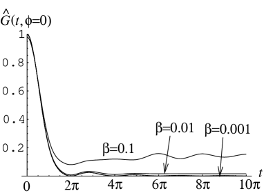
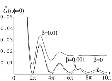
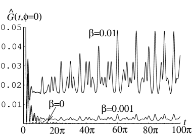
Figure 1: The normalized correlation function $\hat{G}_{(N_{n\mu},N_{n\mu}^{\prime})}(t,\phi=0;\beta)$ as a function of time $t$ for various values of the temperature $\beta$. The graph is reproduced from [24] with kind permission of the authors.

The main difference between this system and the free boson is that the D1–D5 system has a much greater degeneracy of states at a given energy scale. This is due to fractionation: whereas for the free boson the energies come naturally in units of $\frac{1}{R}$, for the D1–D5 system the unit size is $\frac{1}{N_{5}R}$, where $R$ is the size of the $S^{1}$ factor. The reason for this is most easily understood by performing a U-duality on the D1–D5 system, which results in an FP system in type II, with a fundamental string wound $N_{5}$ times the $S^{1}$ and $N_{1}$ units of momentum going around the string. Since the total length of the string is $N_{5}R$, the energies associated to this system are naturally quantized in units of $\frac{1}{N_{5}R}$. Mathematically this translates to having fractional frequencies in the correlator (4.6), whereas for the free boson the frequencies were integral (3.5).

4.2 Euclidean variance

We now wish to analyze the variance and the standard deviation to mean ratio of the correlator (4.6) in both real and imaginary time. We start by rotating to Euclidean time by $t\to-i\tau$. Using the well known results for the canonical variances of the Bose–Einstein and Fermi–Dirac distributions,

$$\textrm{var}(N_{n\mu})_{can}=\frac{1}{4\sinh^{2}\frac{\beta n}{2}},\quad\textrm{var}(N_{n\mu}^{\prime})_{can}=\frac{1}{4\cosh^{2}\frac{\beta n}{2}},$$ (4.7)

we can compute the variance of the Euclidean correlator. It is given by

$$\textrm{var}(\hat{G}_{(N_{n\mu},N_{n\mu}^{\prime})}(\tau))_{can}=\frac{64\beta^{4}}{\pi^{4}}\sinh^{4}\frac{\tau}{2}\sum_{n=1}^{\infty}\frac{1}{n^{2}\sinh^{4}\frac{\tau}{n}}\left(1+\frac{\sinh\tau}{n\tanh\frac{\tau}{n}}\right)^{2}\frac{\cosh\beta n}{\sinh^{2}\beta n}.$$ (4.8)

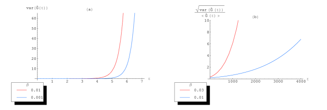
Figure 2: (a): Variance as a function of Euclidean time. The ‘temperatures’ are $\frac{1}{\beta}=100$ (left) and $1000$ (right). (b): Standard deviation to mean–ratio as a function of Euclidean time for ‘temperatures’ $\frac{1}{\beta}=\frac{100}{3}$ (upper) and $100$ (lower).

As indicated by figure 2, this variance is exponentially growing and the time $\tau_{0}$ when it begins to grow rapidly is much smaller than $\frac{1}{\beta}$. Analyzing the sum in this regime, $1\ll\tau\ll\frac{1}{\beta}$, one can see that it is dominated by terms with $n\sim\mathcal{O}(\frac{1}{\beta})$, for which the terms behave like $\frac{1}{64}\beta^{2}\frac{e^{4\tau}}{\tau^{6}}$. Since there are $\mathcal{O}(\frac{1}{\beta})$ of these we see that the variance approximately behaves as

$$\textrm{var}(\hat{G}_{N_{n\mu},N_{n\mu}^{\prime}}(\tau))_{can}\sim\frac{1}{\pi^{4}}\beta\frac{e^{4\tau}}{\tau^{6}}.$$ (4.9)

From this we can conclude that the relevant timescale for rapid growth of the variance is given approximately as $\frac{1}{4}\ln\frac{1}{\beta}\sim\ln N^{\frac{1}{8}}\sim\ln S^{\frac{1}{4}}$.

However, the quantity that measures the size of fluctuations in the ensemble is the standard deviation to mean-ratio. Using results from above we can easily compute this to be

$$\frac{\sqrt{\textrm{var}(\hat{G}_{E}(\tau))_{can}}}{\langle\hat{G}_{E}(\tau)\rangle}=\frac{\sqrt{\sum_{n=1}^{\infty}\frac{1}{n^{2}\sinh^{4}\frac{\tau}{n}}\left(1+\frac{\sinh\tau}{n\tanh\frac{\tau}{n}}\right)^{2}\frac{\cosh\beta n}{\sinh^{2}\beta n}}}{\sum_{n}^{\infty}\frac{1}{n\sinh^{2}\frac{\tau}{n}}\left(1+\frac{\sinh\tau}{n\tanh\frac{\tau}{n}}\right)\frac{1}{\sinh\beta n}}.$$ (4.10)

This is also plotted in figure 2 and also exhibits exponential growth. However, the relevant timescales are now much longer: $\tau\gg\frac{1}{\beta}$. Analyzing the sums in this regime we find that they are dominated by terms with $n\sim\mathcal{O}(\tau)$, which contribute as

$$\frac{\sqrt{\textrm{var}(\hat{G}_{E}(\tau))_{can}}}{\langle\hat{G}_{E}(\tau)\rangle}\approx\frac{\frac{1}{\tau^{\frac{3}{2}}}e^{(1-\frac{\beta}{2})\tau}}{\frac{1}{\tau}e^{(1-\beta)\tau}}=\frac{e^{\frac{\beta\tau}{2}}}{\sqrt{\tau}},$$ (4.11)

showing that the time scales are indeed much larger, as they are now in units of $\frac{1}{\beta}\sim S$. This is not the whole story, though. As with the toy model of the free boson, the correct ensemble to use is the ensemble of all possible superpositions of ground states (4.2). This will again give an additional suppression by $e^{S}$ to the result computed above, and the standard deviation to mean-ratio will behave as

$$\frac{\sqrt{\textrm{var}(\hat{G}_{E}(\tau))_{{\cal M}_{sup}}}}{\langle\hat{G}_{E}(\tau)\rangle}\approx\frac{e^{\frac{\beta\tau}{2}}}{e^{\frac{S}{2}}\sqrt{\tau}}=\frac{e^{\frac{\beta\tau-\frac{1}{\beta}}{2}}}{\sqrt{\tau}},$$ (4.12)

showing that the timescale in imaginary time for distinguishing different microstates will be $\tau\sim\frac{1}{\beta^{2}}\sim S^{2}$. Note also that the absence of periodicity in imaginary time immediately distinguishes correlation functions computed in a microstate from correlation functions computed in the thermal ensemble.

4.3 Lorentzian variance

It can be readily shown that the Lorentzian variance decreases as $N$ increases, and vanishes in the large $N$ limit. The quantity of interest for us is the standard deviation to mean ratio. In this case the ratio can be computed using (4.7) and (4.6), and one finds

$$\mathcal{F}(t)\equiv\frac{\sqrt{\textrm{var}(\hat{G}(t))_{can}}}{\langle\hat{G}(t)\rangle}=\frac{\sqrt{\sum_{n=1}^{\infty}n^{2}f_{n}(t)^{2}\frac{\cosh\beta n}{\sinh^{2}\beta n}}}{\sum_{n=1}^{\infty}nf_{n}(t)\frac{1}{\sinh\beta n}},\quad\textrm{where }f_{n}(t)=\left(\frac{\sin\frac{t}{2}}{n\sin\frac{t}{n}}\right)^{2}\left(1+\frac{\sin t}{n\tan\frac{t}{n}}\right).$$ (4.13)

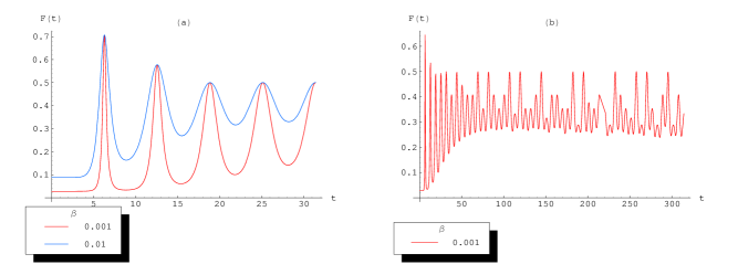
Figure 3: The standard deviation to mean ratio $\mathcal{F}(t)$ in real time. (a): Short time scale behaviour, plotted for $\frac{1}{\beta}=100$ (upper) and $\frac{1}{\beta}=1000$ (lower)). (b): Long time behaviour plotted for $\frac{1}{\beta}=1000$)

This quantity is plotted for small and large timescales in figure 3, which shows quasi-periodic oscillations of period $2\pi$. To understand this behavior, we need to know which terms contribute to the sums, and how the functions $f_{n}(t)$ behave.

Firstly, the terms are suppressed by $\frac{1}{\sinh\beta n}$, and therefore for high $n$ the terms are negligible. Thus it is enough to include only $\mathcal{O}(\frac{1}{\beta})=\mathcal{O}(\sqrt{N})$ first terms. Also, for small values of $n$ we can approximate $\frac{\cosh\beta n}{\sinh^{2}\beta n}\approx\frac{1}{\sinh^{2}\beta n}$, showing that these terms in the two sums in (4.13) will scale identically as a function of $\beta$. Thus we see that the terms that determine the behavior of the ratio as a function of $\beta$ are the intermediate ones: $n\lesssim\sqrt{N}$. The functions $f_{n}(t)$ also play an important role and we must understand their behavior. It is easy to show that these functions fluctuate between 0 and $\frac{1}{2}$ reaching $f_{n}(t)=\frac{1}{2}$ at $t=2nm\pi$, where $m$ is any integer, or also half integer in the case of even $n$.

$\mathcal{F}$ for early times: Let us first analyze the behavior of the ratio around $t=0$. In this case $f_{n}(t)=\frac{1}{2}$ for all $n$, and we can compute the sums by approximating them with integrals:

$$\frac{\sqrt{\textrm{var}(\hat{G}(0))_{can}}}{\langle\hat{G}(0)\rangle}\approx\frac{\sqrt{\frac{1}{\beta^{3}}\int_{0}^{\infty}dxx^{2}\frac{\cosh x}{\sinh^{2}x}}}{\frac{1}{\beta^{2}}\int_{0}^{\infty}dxx\frac{1}{\sinh x}}\approx 0.9\sqrt{\beta}.$$ (4.14)

This indicates that for the earliest times at high temperatures, the fluctuations in this ensemble are small and one can’t tell the thermal state from a typical state.

Peaks: Now let us analyze the peaks that occur at $t=2\pi m$ for integer $m$. At these times both numerators in $f_{n}(t)$ vanish, so to get a non-zero contribution the denominators should vanish as well. This gives the condition $\frac{2\pi m}{n}=p\pi$ for some integer $p$, or equivalently

$$n=\frac{2m}{p}.$$ (4.15)

For the first and highest peak $m=1$, so clearly the only solutions are $n=1,2$. This means that in the sums in (4.13) only the first two terms contribute, giving

$$\left.\frac{\sqrt{\textrm{var}(\hat{G}(t))_{can}}}{\langle\hat{G}\rangle}\right|_{\textrm{first peak}}\approx\frac{\sqrt{\frac{1}{2^{2}}\frac{\cosh\beta}{\sinh^{2}\beta}+2^{2}\frac{1}{2^{2}}\frac{\cosh 2\beta}{\sinh^{2}2\beta}}}{\frac{1}{2}\frac{1}{\sinh\beta}+2\frac{1}{2}\frac{1}{\sinh 2\beta}}\approx\frac{\sqrt{2}}{2}\approx 0.707,$$ (4.16)

which matches well with the plot in figure 3. Note that the height of the peak is not dependent on the temperature $\frac{1}{\beta}$ for small $\beta$ (large $N$). The other peaks can be analyzed using the same method.

For later times, $t\sim\mathcal{O}(\frac{1}{\beta})$, the number of terms that contribute at the peaks is the number of integers that divide $2m$, which for large $m$ is generically proportional to $\ln{m}$ [31]. In this case the standard deviation to mean ratio goes as

$$\mathcal{F}(t)\approx\frac{\sqrt{(\frac{1}{2})^{2}\frac{1}{(\beta)^{2}}\times\ln\frac{1}{\beta}}}{(\frac{1}{2})\frac{1}{\beta}\times\ln\frac{1}{\beta}}\approx\frac{1}{\sqrt{\ln\frac{1}{\beta}}}\approx\frac{1}{\sqrt{\frac{1}{2}\ln N}},$$ (4.17)

where $\ln\frac{1}{\beta}$ is the number of contributing terms, all of which are roughly the same size. This shows that the height of the peaks decreases as $N\to\infty$, although very slowly. However, even for late times there will be many peaks that remain finite. This is because the number of divisors of $m$ is only very roughly $\ln m$; for instance when $m$ is prime the number of divisors is 2, in which case the multiplicity factor is absent in the computation above and the ratio is finite for all $\beta$.

The $O(1)$ height of the peaks in the standard-deviation to mean ratio might have suggested that the microstates can be easily distinguished from each other and from the thermal ensemble at early timescales. If so this would contradict the finding in [24] that the graviton correlator is universal and largely independent of the twist distribution for a very long period of time, and the result presented there that correlators in the basis microstates agree with the BTZ result for a time of order $1/\beta\sim\sqrt{N}\sim S$. The potential tension is resolved, because it can be shown that in the small $\beta$ (large $N$) limit that is relevant for the validity of classical geometry, at the times $t=2\pi m$ the mean correlator actually vanishes. Hence although the standard deviation to mean ratio is nominally of $O(1)$ at these instants, the variation between microstates will not be measurable without very high precision. Likewise, notice from Fig. 3 that the width in the peaks of the standard-deviation to mean ratio become narrower as $\beta$ decreases. This indicates that in addition to precision of measurement, high temporal resolution would also be needed to resolve the differences in the correlators between different basis microstates in the ensemble $\mathcal{M}_{bas}$. In any case, as we will see in the ensemble of all microstates (i.e. including superpositions of the basis elements) the standard deviation to mean ratio will be enormously suppressed.

There is one more timescale that is of interest to us. As pointed out in [24], for any finite $N$ only a finite number of the twist operators are present, and therefore there is only a finite number of frequencies present in correlator (4.6). Thus the system will exhibit exact periodicity at timescales when $t$ is of the order of the lowest common multiple of the frequencies. This timescale was shown to increase as $e^{\sqrt{N}}\sim e^{S}$, and thus the period for this system will be roughly the Poincaré recurrence time, as expected.

Suppression: Finally, as argued in Sec. 2, the correct ensemble to use is $\mathcal{M}_{sup}$, the ensemble containing the superpositions of the basis states. In this ensemble the variance is suppressed by a factor of $e^{S}$ from the one computed in the ensemble $\mathcal{M}_{bas}$, and taking this into account, we see that the standard deviation to mean ratio computed in (4.13) needs to divided by $e^{\frac{S}{2}}$, making it virtually vanish. Due to the analysis above we know that the ratio never grows appreciably, from which we can conclude that the fluctuations in the ensemble of superpositions are too small to be detected by any semiclassical measurement, and therefore one cannot hope to tell different microstates apart from each other.

Summary of the D1-D5 system:

We have shown that in the D1-D5 system the individual microstates can be distinguished from the $M=0$ BTZ geometry by excursions of the correlation functions into the complex plane. Despite the entropic suppression of the variance we find that at imaginary timescales $\tau\sim S^{2}$ there is a distinction between the microstates and the black hole geometry. On the other hand it is virtually impossible to tell apart the states from each other in real time since the exponential suppression of the variance overwhelms the deviations in the correlation functions. The natural timescale over which we can tell apart states is expected to be $t\sim e^{S}$ – the Poincaré recurrence time (cf., [10]).

5 Discussion

Our principal finding is that the variances of local correlation functions computed in generic microstates of a system with entropy $S$ are suppressed by a factor of $e^{-S}$. This is a general result arising from statistical considerations and is true both for free and interacting theories regardless of the strength of the coupling. Our results were illustrated in two examples: the 1+1 dimensional free boson and the D1-D5 CFT which is dual to the BTZ black hole. Applied to black holes it implies that extreme precision (and correspondingly long measurement timescales) are necessary to distinguish microstates from each other. Thus our results suggest that even if there are non-singular, horizon free black hole microstates as proposed in [2], they are universally described by the semiclassical, coarse-grained observer in terms of the conventional black hole geometries.

In our two examples we investigated whether the structure of correlation functions in imaginary time can better separate microstates from each other and from the thermal average. Certainly the thermal average correlator differs from the answer in any individual microstate because the former must be periodic in imaginary time. In particular, the correlation function at zero spatial separation must therefore diverge at $\tau=\beta$ in the thermal ensemble, while it is finite for a generic microstate. Furthermore, while we have seen that the variances in the correlation functions are exponentially suppressed, making it impossible to distinguish different states in real time-scales less than the Poincaré time $t\sim e^{S}$, correlation functions grow exponentially in imaginary time, which possibly increases the differences between distinct microstates. While it is not clear that analytically continued correlation functions are accessible to a single observer, we should emphasize that the discussion above indicates an in-principle possibility of being able to access the information and hence being able to distinguish microstates.

It is worth emphasizing that in this picture, individual microstates of fixed energy do not correspond to an eternal black hole geometry. This is because correlators computed in a single asymptotic region of the latter are automatically periodic in imaginary time, unlike the correlators in individual microstates. Thus, we must conclude that the canonical (fixed temperature) and microcanonical (fixed energy) ensembles in a CFT are not dual to eternal black holes as they are sometimes taken to be. Rather, the ensemble in the CFT is dual to an ensemble of microstate spacetimes which may or may not have a description purely in geometry, but certainly do not have two asymptotic regions and imaginary time periodicity of correlators. However, our findings imply that a semiclassical observer with access only to coarse-grained observables would be able to describe his or her findings approximately in terms of a BTZ geometry.

Finally, our analysis shows the exponential suppression of variances for finitely local correlation functions; the explicit calculations used specific local correlators that were easy to compute. One might ask if there are other observables that can separate the microstates more easily. For example, nonlocal observables like Wilson loops are infinite sums of local correlators and have been argued to be effective at probing the underlying states of black holes [33]. Our finding that the variance in correlators is amplified in imaginary time has a related character because to determine the correlator everywhere in the complex plane from measurements just along the real line will require knowledge of an infinite number of derivatives.

Acknowledgments:

We have enjoyed useful discussions with Vishnu Jejjala, Per Kraus, Hong Liu, Steve Shenker and Masaki Shigemori. Some of the work in this paper was done at the 2006 Aspen workshop on black hole physics, the 2006 Indian String Meeting, the 2007 KITP miniprogram on the quantum nature of singularities, and under a banyan tree at the Konarak temple. VB, BC, KL and JS were supported in part by DOE grant DE-FG02-95ER40893. JS was supported in part by DOE grant DE-AC03-76SF00098 and NSF grant PHY-0098840. This research was also supported in part by the National Science Foundation under Grant No. PHY99-07949.

Appendix A Ensembles with fixed energy expectation values

We have considered ensembles of states in which the energy eigenvalues fall between $E$ and $E+\Delta E$. One might have considered an ensemble of states in which only the expectation values are so bounded, i.e.

$${\cal M}_{exp}=\left\{\ |\psi\rangle\ :\ E\leq\,\langle\,\psi|H|\psi\,\rangle\,\leq E+\Delta E\ \right\}\,.$$ (A.1)

The states $|\psi\rangle$ could then be superpositions of energy eigenstates with arbitrarily high eigenvalues. For example, we could take

$$|\psi\rangle=(1-\epsilon)^{1/2}\,|0\rangle+\epsilon^{1/2}\,|s\rangle\ \ \Longrightarrow\ \ \langle\psi|\,H\,|\psi\rangle=\epsilon\,e_{s}=E$$ (A.2)

with $e_{s}\gg E$ and $\epsilon=E/e_{s}$. In general if we take $|\psi\rangle=\sum_{s}c_{s}|s\rangle$ to be an element of ${\cal M}_{exp}$ written as a sum of energy eigenstates, then we require that

$$E\leq\sum_{s}|c_{s}|^{2}\,e_{s}\leq E+\Delta E\,.$$ (A.3)

Since this is not a linear constraint on the coefficients $c_{s}$, it is not possible to write a linear basis of states for all elements of the ensemble ${\cal M}_{exp}$; i.e. they do not form a Hilbert space. Of course the superposition coefficients of the eigenstates with energies much bigger than $E$ will have to be small, but observables such as $H^{k}$ for large $k$ will be increasingly sensitive to the energy components of states lying outside the range $E\leq e_{s}\leq E+\Delta E$.

In view of this, the essential finding – that the variance over $\mathcal{M}_{sup}$ is suppressed – will apply to this ensemble when probe operators satisfy a Lipschitz condition with respect to energy expectations:

$$|\langle\,\psi\,|\,\mathcal{O}\mid\!\psi\,\rangle-\langle\,\phi\,|\,\mathcal{O}\mid\!\phi\,\rangle|<L\,|\langle\,\psi\,|\,H\mid\!\psi\,\rangle-\langle\,\phi\,|\,H\mid\!\phi\,\rangle|$$ (A.4)

for some constant $L$. To see this, consider a family of states $|E\rangle$, parametrized by the real scalar $b$:

$$\mid\!E\,\rangle=\sqrt{\frac{b-E}{b-a}}\mid\!a\,\rangle+\sqrt{\frac{E-a}{b-a}}\mid\!b\,\rangle,$$ (A.5)

with:

$${\langle\,E\,|\,H\mid\!E\,\rangle}$$

(A.6)

In the above, the fixed constant $a$ is an energy close to but lower than $E$

$$E-\Delta E<a<E$$ (A.7)

while the parameter $b$ must be greater than $E$ but is otherwise unconstrained. Then:

$${\langle\,E\,|\,\mathcal{O}\mid\!E\,\rangle}$$

(A.8)

In this way, the Lipschitz condition will bound discrepancies in means and variances between the ensembles ${\cal M}_{exp}$ and ${\cal M}_{sup}$ to $\mathcal{O}(\Delta E)$.

Appendix B Derivation of the “thermal state”

The occupation numbers $N_{n}$, which characterize elements of the ensemble $\mathcal{M}_{bas}$, satisfy $\sum nN_{n}=E$ and therefore admit a representation in terms of Young tableaux $\mu$. Such tableaux are conveniently described in a coordinate system, where the horizontal axis $y$ spans the indices of the bosonic oscillators, while the abscissa $x$ measures the cumulative population of all the oscillators from infinity down to $y(x)$:

$$x(y)=\int_{y}^{\infty}N_{n}\,dn\,.$$ (B.1)

Using canonical ensemble methods, Vershik showed [34] that for large $E$, almost all states (elements of $\mathcal{M}_{bas}$) lie close to the limit shape given by:

$$\exp{(-x\sqrt{\zeta(2)/E})}+\exp{(-y\sqrt{\zeta(2)/E})}=1\,.$$ (B.2)

The curve (B.2) may be thought of as the average of the ensemble $\mathcal{M}_{bas}$, and as such it should be identified with the thermal state (3.6). This is accurate for regimes where the canonical and the microcanonical treatments agree, i.e. for $x,\,y\approx\sqrt{E}$, which is where most of the entropy lies. The occupation numbers obtained from the limit curve take the form

$$N_{n}=-\frac{dx}{dy}\biggr{|}_{y=n}\;=\;{1\over\exp{(n\sqrt{\zeta(2)/E})}-1}\,,$$ (B.3)

leading to the identification:

$$\beta=\sqrt{\frac{\zeta(2)}{E}}\,.$$ (B.4)

The entropy, given by the asymptotic total number of partitions of $E$ due to Hardy and Ramanujan [35], takes the form:

$$S=\frac{2\,\zeta(2)}{\beta}+\mathcal{O}(\log{\beta})\,.$$ (B.5)

Appendix C Taxonomy of possible configurations

We collect in this appendix the various states and ensembles that are used in the main discussion. Since one is generically interested in telling apart microstates from each other and from the black hole it is useful to keep the subtle distinctions described below in mind while referring to various macroscopic configurations.

Ensembles:

1. Canonical or thermal ensemble: This is the ensemble of states in the Hilbert space with the probability of finding an energy eigenstate of energy $E$ is given by $e^{-\beta E}$. This ensemble is best thought of for measurement purposes in the quantum cosmological sense. Each measurement gives us the eigenvalues of the probe, subject to the fact that the intrinsic probability distribution of states is given by the canonical distribution.

2. Microcanonical basis ensemble, $\mathcal{M}_{bas}$: This is the ensemble defined in (2.1), where we restrict attention to the basis of energy eigenstates (which for the cases of interest are also number operator eigenstates), with each element being equally probable in the ensemble. The ensemble has $e^{S}$ elements.

3. Microcanonical superposition ensemble, $\mathcal{M}_{sup}$: This is the ensemble defined in (2.2), where we allow arbitrary superpositions of energy eigenstates, appropriately normalized.

States:

1. Hartle-Hawking state: This is a pure entangled state that is constructed in the tensor product of two copies of the Hilbert space. The entanglement is fine tuned so that we reproduce the average values of the canonical ensemble after tracing over one of the Hilbert spaces. This is the description of the eternal Schwarzschild-AdS black hole.

2. “Thermal state”: The “thermal state” a formal construct; it doesn’t belong to any of the ensembles described above which reproduces thermal averages. This is the state whose derivation was explained in Appendix  B.

3. Typical microstate: The typical microstate is an element of $\mathcal{M}_{sup}$ whose occupation numbers are tuned by choice of the superposition coefficients to come arbitrarily close to mimic the “thermal state”, although only up to the energy of the ensemble $\mathcal{M}_{sup}$.

4. Typical basis microstates: These states are elements of $\mathcal{M}_{bas}$, with integral occupation numbers which lie close to the typical microstate. In the geometric picture they are usually associated with the microstate geometries of [2].

References

- [1]
- [2] O. Lunin and S. D. Mathur, “AdS/CFT duality and the black hole information paradox,” Nucl. Phys. B 623, 342 (2002) [arXiv:hep-th/0109154]; S. D. Mathur, “The fuzzball proposal for black holes: An elementary review,” Fortsch. Phys. 53, 793 (2005) [arXiv:hep-th/0502050].
- [3]
- [4] H. Lin, O. Lunin and J. M. Maldacena, “Bubbling AdS space and 1/2 BPS geometries,” JHEP 0410, 025 (2004) [arXiv:hep-th/0409174].
- [5]
- [6] V. Balasubramanian, J. de Boer, V. Jejjala and J. Simon, “The library of Babel: On the origin of gravitational thermodynamics,” JHEP 0512, 006 (2005) [arXiv:hep-th/0508023]; V. Balasubramanian, V. Jejjala and J. Simon, “The library of Babel,” Int. J. Mod. Phys. D 14, 2181 (2005) [arXiv:hep-th/0505123].
- [7]
- [8] I. Bena and N. P. Warner, “Bubbling supertubes and foaming black holes,” Phys. Rev. D 74, 066001 (2006) [arXiv:hep-th/0505166]; P. Berglund, E. G. Gimon and T. S. Levi, “Supergravity microstates for BPS black holes and black rings,” JHEP 0606, 007 (2006) [arXiv:hep-th/0505167]; I. Bena, C. W. Wang and N. P. Warner, “The foaming three-charge black hole,” arXiv:hep-th/0604110. V. Balasubramanian, E. G. Gimon and T. S. Levi, “Four dimensional black hole microstates: From D-branes to spacetime foam,” arXiv:hep-th/0606118. I. Bena, C. W. Wang and N. P. Warner, “Mergers and typical black hole microstates,” JHEP 0611, 042 (2006) [arXiv:hep-th/0608217].
- [9]
- [10] V. Balasubramanian, D. Marolf and M. Rozali, “Information recovery from black holes,” [arXiv:hep-th/0604045]; V. Balasubramanian, B. Czech, K. Larjo and J. Simon, “Integrability vs. information loss: A simple example,” JHEP 0611, 001 (2006) [arXiv:hep-th/0602263].
- [11]
- [12] L. F. Alday, J. de Boer and I. Messamah, “The gravitational description of coarse grained microstates,” arXiv:hep-th/0607222.
- [13]
- [14] D. Berenstein, “Large N BPS states and emergent quantum gravity,” JHEP 0601, 125 (2006) [arXiv:hep-th/0507203]; S. E. Vazquez, “Reconstructing 1/2 BPS space-time metrics from matrix models and spin chains,” arXiv:hep-th/0612014.
- [15] P. Kraus, H. Ooguri and S. Shenker, “Inside the horizon with AdS/CFT,” Phys. Rev. D 67, 124022 (2003) [arXiv:hep-th/0212277].
- [16] L. Fidkowski, V. Hubeny, M. Kleban and S. Shenker, “The black hole singularity in AdS/CFT,” JHEP 0402, 014 (2004) [arXiv:hep-th/0306170].
- [17] T. S. Levi and S. F. Ross, “Holography beyond the horizon and cosmic censorship,” Phys. Rev. D 68, 044005 (2003) [arXiv:hep-th/0304150]; V. Balasubramanian and T. S. Levi, “Beyond the veil: Inner horizon instability and holography,” Phys. Rev. D 70, 106005 (2004) [arXiv:hep-th/0405048].
- [18] D. Brecher, J. He and M. Rozali, “On charged black holes in anti-de Sitter space,” JHEP 0504, 004 (2005) [arXiv:hep-th/0410214].
- [19] G. Festuccia and H. Liu, “Excursions beyond the horizon: Black hole singularities in Yang-Mills theories. I,” JHEP 0604, 044 (2006) [arXiv:hep-th/0506202].
- [20] B. Freivogel, V. E. Hubeny, A. Maloney, R. Myers, M. Rangamani and S. Shenker, “Inflation in AdS/CFT,” JHEP 0603, 007 (2006) [arXiv:hep-th/0510046].
- [21] K. Maeda, M. Natsuume and T. Okamura, “Extracting information behind the veil of horizon,” Phys. Rev. D 74, 046010 (2006) [arXiv:hep-th/0605224].
- [22] A. Hamilton, D. Kabat, G. Lifschytz and D. A. Lowe, “Local bulk operators in AdS/CFT: A holographic description of the black hole interior,” arXiv:hep-th/0612053.
- [23] J. M. Maldacena, “Eternal black holes in Anti-de-Sitter,” JHEP 0304, 021 (2003) [arXiv:hep-th/0106112].
- [24] V. Balasubramanian, P. Kraus and M. Shigemori, “Massless black holes and black rings as effective geometries of the D1-D5 system,” Class. Quant. Grav. 22, 4803 (2005) [arXiv:hep-th/0508110].
- [25] H. Elvang, R. Emparan, D. Mateos and H. S. Reall, “Supersymmetric black rings and three-charge supertubes,” Phys. Rev. D 71, 024033 (2005) [arXiv:hep-th/0408120].
- [26] L. F. Alday, J. de Boer and I. Messamah, “What is the dual of a dipole?,” Nucl. Phys. B 746, 29 (2006) [arXiv:hep-th/0511246].
- [27] S. W. Hawking and D. N. Page, “Thermodynamics Of Black Holes In Anti-De Sitter Space,” Commun. Math. Phys. 87, 577 (1983).
- [28] R. M. Wald, “The thermodynamics of black holes,” Living Rev. Rel. 4, 6 (2001) [arXiv:gr-qc/9912119].
- [29] K. Skenderis and M. Taylor, “Fuzzball solutions and D1-D5 microstates,” [arXiv:hep-th/0609154].
- [30] O. Lunin and S. D. Mathur, “Correlation functions for M(N)/S(N) orbifolds,” Commun. Math. Phys. 219, 399 (2001) [arXiv:hep-th/0006196]; O. Lunin and S. D. Mathur, “Three-point functions for M(N)/S(N) orbifolds with N = 4 supersymmetry,” Commun. Math. Phys. 227, 385 (2002) [arXiv:hep-th/0103169].
- [31] G. L. Dirichlet, ”Sur l’usage des séries infinies dans la théorie des nombres,” J. reine angew. Math. 18, 259-274, 1838.
- [32] G. Festuccia and H. Liu, “The arrow of time, black holes, and quantum mixing of large N Yang-Mills theories,” arXiv:hep-th/0611098.
- [33] V. E. Hubeny, “Precursors see inside black holes,” Int. J. Mod. Phys. D 12, 1693 (2003) [arXiv:hep-th/0208047]; L. Susskind and N. Toumbas, “Wilson loops as precursors,” Phys. Rev. D 61, 044001 (2000) [arXiv:hep-th/9909013].
- [34] A.M.Vershik, ”Statistical mechanics of combinatorial partitions, and their limit configurations,” Funkts. Anal. Prilozh. 30, No.2, 19-30 (1996) (English translation: Funct. Anal. Appl. 30, No.2, 90-105 (1996)).
- [35] G. H. Hardy, S. Ramanujan, ”Asymptotic Formulae in Combinatory Analysis,” Proc. London Math. Soc. 17, 75-115, 1918.