Alternative representation for non–local operators and path integrals

Abstract

We derive an alternative representation for the relativistic non–local kinetic energy operator and we apply it to solve the relativistic Salpeter equation using the variational sinc collocation method. Our representation is analytical and does not depend on an expansion in terms of local operators. We have used the relativistic harmonic oscillator problem to test our formula and we have found that arbitrarily precise results are obtained, simply increasing the number of grid points. More difficult problems have also been considered, observing in all cases the convergence of the numerical results. Using these results we have also derived a new representation for the quantum mechanical Green’s function and for the corresponding path integral. We have tested this representation for a free particle in a box, recovering the exact result after taking the proper limits, and we have also found that the application of the Feynman–Kac formula to our Green’s function yields the correct ground state energy. Our path integral representation allows to treat hamiltonians containing non–local operators and it could provide to the community a new tool to deal with such class of problems.

I Introduction

The appearance of non–local operators in the relativistic extensions of the Schrödinger equation poses a serious challenge both to analytical and numerical calculations. However, the inclusion of relativistic effects is crucial for example in the study of meson phenomenology, where the Bethe-Salpeter equation (BSE) provides the correct theoretical tool to describe relativistic bound states. Replacing the kernel in the BSE with an instantaneous local potential one obtains a relativistic Schrödinger equation, which is also known as “spinless Salpeter equation” (SSE). In such case the hamiltonian operator is typically given by

$$\hat{H}=\sqrt{\hat{p}^{2}+m^{2}}+V(\vec{r})\ .$$ (1)

From a technical point of view, the inclusion in the Hamiltonian of the relativistic kinetic energy operator, $\sqrt{\hat{p}^{2}+m^{2}}$, complicates the solution of the problem because of its non–local nature. The great phenomenological relevance of the SSE has motivated in the past twenty years many efforts to solve this equation, either using analytical or numerical techniques. Early work on this subject is contained for example in Durand84 ; Long84 ; Lucha92 ; Fulcher94 ; Maung94 . The method described in Fulcher94 , which allows one to obtain a matrix representation of the non-local kinetic energy operator, has also been used recently Semay05 in conjunction with the Lagrange mesh method. In this case, the method is particularly appealing since it does not require the evaluation of the matrix elements of the potential, but rather only the specification of the potential on the grid points. This feature is also shared by the so called sinc collocation methods (see for example Amore06a ; Amore06b ), which could also be used straightforwardly together with the method of Fulcher94 : however we do not consider this possibility since we are rather interested in developing a completely new approach, as it will soon become clear.

In a series of recent works, Lucha and collaborators have been able to obtain precise upper and lower bounds to the eigenvalues of the RSE, Lucha96 ; Lucha00 ; Lucha01 ; Lucha05a : these bounds provide useful analytic or semi–analytic expressions and have been applied to a number of test problems (see for example Lucha05a ). Another approach has been followed in Lucha95 , where an effective hamiltonian of non-relativistic form, which includes relativistic effects by means of parameters depending on the momentum, was constructed.

Finally, the SSE was also studied in the case of the relativistic harmonic oscillator (RHO) in three recent papers, Znojil96 ; Mustafa99 ; Lucha05b . In Lucha05b the authors were able to obtain recurrence relations for the coefficients of the series defining the eigenfunctions. The reader can also find useful the detailed bibliographic information contained in that paper.

The main purpose of the present paper is to develop a completely new approach to the solution of the SSE: we will derive an analytical representation of the non–local kinetic energy operator and use it with the Variational Sinc collocation Method (VSCM) Amore06a to obtain arbitrarily precise numerical results. We will use the RHO of Lucha05b , for which semi–analytical results are available, to test our approach. The new representation that we have found for the relativistic kinetic energy operator has also been generalized to the calculation of the quantum mechanical Green’s function and has allowed us to obtain a new formula, which differs from the standard formula of path integrals.

The paper is organized as follows: in Section II we describe the SSE for the RHO and obtain precise numerical solutions working in momentum space configuration (these results are then compared with the results of Lucha05b ); in Section III we obtain an explicit analytical expression for the matrix elements of the non–local kinetic energy operator in terms of the so called “little sinc functions” (LSF) recently studied in Amore06b (these functions were first introduced by Schwartz in Schwartz85 and later used by Baye in Baye95 ); we use this representation in the VSCM working in coordinate space and reproduce the results previously obtained in momentum space; in Section IV we extend our method to obtain explicit analytical representation for the Green’s function which holds for general potentials; finally in Section V we draw our conclusions and set the direction for future work.

II The Relativistic Harmonic Oscillator

The RHO problem corresponds to the case in which a spherical harmonic oscillator potential, $V(\vec{r})=ar^{2}$, is used in the Hamiltonian of eq. (1). After a simple rescaling of the mass and of the energy the Schrödinger equation can be cast in the form

$$\left[\sqrt{\hat{p}^{2}+\mu^{2}}+r^{2}\right]|\psi\rangle=\varepsilon\ |\psi\rangle\ ,$$ (2)

depending on a single parameter $\mu$ . The advantage of considering this potential lies in the fact that the corresponding Schrödinger equation in momentum space representation is local and it can therefore be attacked with standard techniques. In this case we are left with the equation

$$\left[-\Delta_{p}+\sqrt{p^{2}+\mu^{2}}\right]\varPsi(p)=\varepsilon\ \varPsi(p)\ ,$$ (3)

where $\Delta_{p}\equiv\frac{\partial^{2}}{\partial p_{x}^{2}}+\frac{\partial^{2}}{\partial p_{y}^{2}}+\frac{\partial^{2}}{\partial p_{z}^{2}}$.

The authors of Lucha05b focus their analysis on the $l=0$ solutions and obtain a recurrence relation for the coefficients of the reduced radial wave function $y(p)=\sqrt{4\pi}p\ \varPsi(p)$. The same problem has also been discussed by M. Trott in Trott , using a basis of harmonic oscillator wave functions in momentum space and numerically computing in this basis the matrix element $\langle i|\sqrt{-\partial_{x}^{2}+m^{2}}|j\rangle$.

We will use the VSCM of Amore06a ; Amore06b to obtain a numerical solution of the problem and then compare our solution with the results of Lucha05b . The VSCM uses sinc functions (SF), defined on the real line, or “little sinc functions” (LSF)Amore06b , a particular generalization of sinc functions defined on finite intervals, to solve the Schrödinger equation by a collocation technique. Since the details of this method are clearly explained in Amore06a ; Amore06b , we will here avoid mentioning all the technical details focusing on giving a more qualitative picture.

SF and LSF are functions which are strongly peaked around a certain value and they fastly decay and oscillate, when moving away from this value. Under certain conditions they can be chosen to be orthogonal: such set of orthogonal functions is obtained by performing a replica of one function at the points where this function vanishes, thus effectively introducing a grid. Unless otherwise specified, either by the Physics of the problem or by convention, the spacing of the grid is arbitrary and, if not carefully chosen, it strongly affects the precision of the results. In a recent paper Amore et al. have used an arbitrary scale factor as a variational parameter in the solution of the Schrödinger equation using a basis of simple harmonic oscillator wave functions Amore05a : in that case it was shown that the optimal scale factor could be chosen to minimize the trace of the Hamiltonian matrix in the Hilbert subspace spanned by the $N$ elements of the basis. The same principle, which was inspired by the Principle of Minimal Sensitivity (PMS) Ste81 , was then used in Amore06a ; Amore06b using a sinc collocation technique. As mentioned in the Introduction the sinc collocation has the great advantage of avoiding the evaluation of matrix elements of the potential, which is simply “collocated” at the grid points; on the other hand the evaluation of the matrix elements of the non–relativistic kinetic operator is also quite simple, since it involves matrices whose elements are obtained by collocating the derivative of a given sinc function at the grid points. In this way one easily obtains a matrix representation for the Hamiltonian.

For example in one dimension one has

$$H_{kl}=-\frac{\hbar^{2}}{2m}c_{kl}^{(2)}+\delta_{kl}V(kh)\ .$$ (4)

where $c^{(2)}$ is the matrix obtained from the second derivative of the sinc functions. $h$ is the grid spacing. In the following we will set $\hbar=1$, so that $h$ will not be confused with the Planck constant.

The diagonalization of $H$ allows one to obtain the eigenvalues (energies) and the eigenvectors (wave functions) of the problem (the number of these eigenvalues and eigenvectors being equal to the number of sinc functions used).

Before trying to deal with the RHO in coordinate space, where it is non–local, we wish to use the VSCM to find numerical solutions in momentum space, where it is local. In this case machinery of VSCM applies straightforwardly and we are able to verify our claim of accuracy of our method. To allow a comparison with Lucha05b we have used $\mu=30$ and calculated the values of $\varepsilon-\mu$ for $\mu=30$ using grids with different $N$. The optimal region in momentum space has been obtained by applying the PMS condition to the problem. Our results show that the method converges quite rapidly; as a matter of fact, for $N=50$ we obtain $\varepsilon-\mu=0.386266042572445193517188444455$ which has all the digits correct and agrees with the result shown in Table 1 of Lucha05b , although the latter contains only $6$ digits.

However we have also performed a more accurate test using the recurrence relations for the coefficients appearing in the series for the wave functions given in Lucha05b . We have extracted these coefficients by expanding around $p=0$ the wave function obtained with our method and we have compared them with the results obtained using directly the recurrence relation of eq.(8) of Lucha05b . In this way we have obtained an indipendent confirmation of the accuracy of our results.

The importance of the RHO lies in the unique possibility of having a complete control on the solutions of the problem, which can be calculated to any desired accuracy, despite retaining the non–local nature of the kinetic energy operator. In more general problems, when the potential is not quadratic in the coordinates, one cannot recover a local Schrödinger equation by working in the momentum space configuration. In these cases one possibility is to resort to a non–relativistic expansion in powers of $p/\mu$, which to lowest order provides the rest mass and the usual non–relativistic kinetic energy:

$$\sqrt{\hat{p}^{2}+\mu^{2}}\approx\mu+\frac{\hat{p}^{2}}{2\mu}+\dots$$ (5)

However the hamiltonian operator obtained in this way contains derivatives of higher order. In such cases it is still possible to apply the VSCM in coordinate space to solve these equations, by using the matrices corresponding to the higher order derivatives (which can be computed quite easily). Although the implementation of this procedure poses no problem, we wish to show that in certain cases it can provide unexpected results, such as results which converge to wrong solutions as the higher order relativistic corrections are added.

We use once again the RHO as our “guinea pig” and work in momentum space configuration using a potential obtained by expanding the kinetic term up to a give order in $p^{2}/\mu^{2}$. The expression in eq. (5), for example, would represent the potential obtained working to order $p^{2}/\mu^{2}$ and corresponds to the usual non–relativistic harmonic oscillator. However, in the inclusion of the higher order terms we have to take into account that terms of order $(p^{2}/\mu^{2})^{2n}$, with $n$ integer, are negative, and therefore one always needs to work to order $(p^{2}/\mu^{2})^{2n+1}$ to have a spectrum bounded from below. We call $\tilde{V}_{2n+1}(p)$ the potential in momentum space corresponding to the expansion to order $(p^{2}/\mu^{2})^{2n+1}$. For example to order $(p^{2}/\mu^{2})^{3}$ we have

$$\tilde{V}_{3}(p)=\mu+\frac{p^{2}}{2\mu}-\frac{p^{4}}{8\mu^{3}}+\frac{p^{6}}{16\mu^{5}}\ .$$ (6)

Once we substitute the non–local operator with its local expansion to a given odd order we can solve the corresponding local Schrödinger equation and thus obtain the energies and the wave functions. We have calculated the values of $\varepsilon-\mu$ for the ground state of the potential using $N=100$ and two different values of $\mu$ ($\mu=30$ and $\mu=5$). In the case corresponding to $\mu=30$ we have observed that the series converges to the exact result within $28$ digit precision for $\tilde{V}_{31}$, while in the case corresponding to $\mu=5$ we have observed that the series does not converge to the exact result, providing its best approximation for $\tilde{V}_{9}$.

We can give a simple explanation of this behavior: for $p>\mu$ the series in eq. (5) – where $p$ is now a real number – diverges and therefore the potential obtained using this series, $\tilde{V}_{\infty}(p)=\lim_{n\rightarrow\infty}\tilde{V}_{2n+1}(p)$, corresponds to the original potential with an infinite wall located at $p=\mu$. In the case $\mu=30$ the wave function is extremely small at $p=\mu$ and therefore the non–relativistic expansion is capable of providing highly (but not arbitrarily) accurate results; on the other hand, in the case $\mu=5$ the wave function is sizeable at $p=\mu$ and the non–relativistic expansion provides a very poor approximation. The situation would clearly get worse as $\mu$ is taken to be smaller.

It should be stressed that in both cases the non–relativistic expansion does converge, although not to the exact result, but rather to a value which depends on the scale $\mu$. I am not aware if this is a well-known fact in the literature.

III Matrix elements of $\sqrt{\hat{p}^{2}+\mu^{2}}$

In this Section we want to describe a new way of calculating the matrix elements of the relativistic kinetic energy operator, which avoids the problems of the local non–relativistic expansion described in the previous Section.

As mentioned in the Introduction, there are approaches in the literature to calculate the matrix elements of this operator, although they are numerical. For example, the method described in Fulcher94 consists of $4$ steps, i.e. the computation of $(K^{2})_{ij}=\langle i|\hat{p}^{2}+\mu^{2}|j\rangle$, the diagonalization of $K^{2}$, the computation of the diagonal square root matrix and finally the computation of the square root matrix $K$. Because of the calculation of $K$ is numerical this procedure would not be profitable in a variational scheme, where the PMS condition is always analytical.

However, we will now show that it is possible to obtain once and for all an analytical representation of $\sqrt{\hat{p}^{2}+\mu^{2}}$ and indeed of any non–local operator which is function of the momentum operator. Because our results will be analytical it will be possible to extend the VSCM to include relativistic non–local terms, in what we will call “Relativistic variational collocation method” (RVSCM).

Let us now present our results. We will work in the following with the Little Sinc Functions (LSF) of Amore06b , although similar results can also be obtained with the usual sinc functions. The LSF have been obtained in Amore06b using the orthonormal basis of the wave functions of a particle in a box with infinite walls located at $x=\pm L$:

$$\psi_{n}(x)=\frac{1}{\sqrt{L}}\ \sin\left(\frac{n\pi}{2L}(x+L)\right)\ .$$ (7)

A LSF is simply obtained as

$$s_{k}(h,N,x) = \frac{2L}{N}\sum_{n=1}^{N}\psi_{n}(x)\psi_{n}(y_{k})\ ,$$ (8)

where $y_{k}\equiv\frac{2kL}{N}=kh$. The LSF should be regarded as an approximate representation of a Dirac delta function. To simplify the notation we have introduced the grid spacing $h\equiv 2L/N$. $k$ is an integer which takes the values $k=-N/2+1,-N/2+2,\dots,N/2-1$, each corresponding to a different grid point.

As shown in Amore06b an explicit expression for the LSF can be obtained for even values of $N$ in the form

$$s_{k}(h,N,x)=\frac{1}{2N}\left\{\frac{\sin\left(\left(1+\frac{1}{2N}\right)\ \frac{\pi}{h}(x-kh)\right)}{\sin\left(\frac{\pi}{2Nh}(x-kh)\right)}-\frac{\cos\left(\left(1+\frac{1}{2N}\right)\ \frac{\pi}{h}(x+kh)\right)}{\cos\left(\frac{\pi}{2Nh}(x+kh)\right)}\right\}\ .$$ (9)

After simple algebra one can also obtain the alternative expression

$$s_{k}(h,N,x)=-\frac{1}{N}\sum_{n=-N}^{+N}(i)^{n+1}\ \sin\left(\frac{n\pi}{2}+\frac{kn\pi}{N}\right)\ e^{i\frac{n\pi x}{2L}}$$ (10)

which is suited to calculate the action of $\sqrt{\hat{p}^{2}+\mu^{2}}$ over a LSF:

$$\sqrt{\hat{p}^{2}+\mu^{2}}\ s_{k}(h,N,x)=-\frac{1}{N}\sum_{n=-N}^{+N}(i)^{n+1}\ \sin\left(\frac{n\pi}{2}+\frac{kn\pi}{N}\right)\ \sqrt{\left(\frac{n\pi}{2L}\right)^{2}+\mu^{2}}\ e^{i\frac{n\pi x}{2L}}\ .$$ (11)

Upon collocation on the grid, i.e. after setting $x\rightarrow x_{j}$, we have the matrix element

$$K_{kj}=\sqrt{\hat{p}^{2}+\mu^{2}}\ s_{k}(h,N,x_{j})=-\frac{1}{N}\sum_{n=-N}^{+N}(i)^{n+1}\ \sin\left(\frac{n\pi}{2}+\frac{kn\pi}{N}\right)\ \sqrt{\left(\frac{n\pi}{2L}\right)^{2}+\mu^{2}}\ e^{i\frac{jn\pi}{N}}\ .$$ (12)

Notice that, despite its appearance, the expression above is real, as it would be evident expressing it in terms of trigonometric functions; however, we prefer to leave it in terms of plane waves.

To check that eq. (12) is indeed the correct matrix element of the non–local kinetic energy operator we can calculate the matrix product $(K^{2})_{kl}=\sum_{j}K_{kj}K_{jl}$

$$(K^{2})_{kl} = \sum_{j}K_{kj}K_{jl}=\frac{1}{N^{2}}\sum_{j=-N/2+1}^{N/2-1}\sum_{n_{1}=-N}^{+N}\sum_{n_{2}=-N}^{+N}(i)^{n_{1}+n_{2}+2}\ \sin\left(\frac{n_{1}\pi}{2}+\frac{kn_{1}\pi}{N}\right)\ \ \sin\left(\frac{n_{2}\pi}{2}+\frac{jn_{2}\pi}{N}\right)$$ (13)

$$\sqrt{\left(\frac{n_{1}\pi}{2L}\right)^{2}+\mu^{2}}\ \sqrt{\left(\frac{n_{2}\pi}{2L}\right)^{2}+\mu^{2}}\ e^{i\frac{(jn_{1}+ln_{2})\pi}{N}}$$

and compare it with the matrix $(K^{2})_{kl}=(\hat{p}^{2}+\mu^{2})_{kl}$, calculated either using the very same eq. (12) with $\sqrt{\left(\frac{n\pi}{2L}\right)^{2}+\mu^{2}}\rightarrow\left(\frac{n\pi}{2L}\right)^{2}+\mu^{2}$ or using the matrix for the second derivative to represent $\hat{p}^{2}$ (see Amore06b ).

We can define

$${\cal C}_{n_{1}n_{2}}\equiv\sum_{j=-N/2+1}^{N/2-1}e^{i\frac{jn_{1}\pi}{N}}\sin\left(\frac{n_{2}\pi}{2}+\frac{jn_{2}\pi}{N}\right)$$ (14)

which for $n_{2}=\pm n_{1}$ takes the values

$${\cal C}_{n_{1}n_{1}}=-{\cal C}_{n_{1},-n_{1}}=-\frac{N}{2}(-i)^{n1+1}\ .$$ (15)

When ${\cal C}_{n1n2}$ is used inside eq. (13) it can be seen that only the terms corresponding to $n_{2}=\pm n_{1}$ contribute, whereas the remaining terms cancel out. In this case we obtain

$$(K^{2})_{kl} = \frac{1}{N^{2}}\sum_{n_{1}=-N}^{+N}\sum_{n_{2}=-N}^{+N}(i)^{n_{1}+n_{2}+2}\ \sin\left(\frac{n_{1}\pi}{2}+\frac{kn_{1}\pi}{N}\right)\ \sqrt{\left(\frac{n_{1}\pi}{2L}\right)^{2}+\mu^{2}}\ \sqrt{\left(\frac{n_{2}\pi}{2L}\right)^{2}+\mu^{2}}\ e^{i\frac{ln_{2}\pi}{N}}$$ (16)

$$\left(-\frac{N}{2}(-i)^{n1+1}\right)\left(\delta_{n_{1},n_{2}}-\delta_{n_{1},-n_{2}}\right)$$

$$= -\frac{1}{N}\sum_{n=-N}^{+N}(i)^{n+1}\ \sin\left(\frac{n\pi}{2}+\frac{kn\pi}{N}\right)\ \left[\left(\frac{n\pi}{2L}\right)^{2}+\mu^{2}\right]\ e^{i\frac{jn\pi}{N}}\ .$$

This completes our proof, since we have precisely obtained the expression that we would have reached if we had used eq. (12) directly with the squared operator. We have also verified numerically this result and confirmed its validity.

As done for the non–relativistic Schrödinger equation we can obtain the Hamiltonian matrix

$$H_{kl}=K_{kl}+\delta_{kl}V(kh)\ .$$ (17)

For a fixed $N$ the matrix elements $H_{kl}$ depend upon the arbitrary scale $L$: as discussed in Amore06a ; Amore06b , it is possible to obtain an optimal value for $L$ by applying the principle of minimal sensitivity (PMS) to the trace of the $N\times N$ hamiltonian matrix ${\cal T}_{N}(L)=Tr\left[\mathbf{H}_{N\times N}\right]$:

$$\frac{d}{dL}{\cal T}_{N}(L)=0.$$ (18)

Physically one can justify this condition by observing that the trace of the hamiltonian is an invariant under unitary transformations and therefore independent of $L$. On the other hand the trace of the truncated matrix does depend on $L$: one can therefore apply the PMS condition (18) to minimize such dependence and thus obtain the scale where the problem is less sensitive to changes in $L$ (normally this equation provides a single solution, although in the case of multiple solutions one would choose the solution corresponding to a flatter curve). Since (18) is an algebraic equation, the computational cost needed in solving it is quite limited. The scale $L$ obtained in this way is then used inside eq. (17) and the hamiltonian matrix is diagonalized, thus providing the $N$ lowest eigenvalues and eigenfunctions. The error corresponding to choosing $L$ according to the PMS is observed to be nearly optimal, leading to results which converge more rapidly as $N$ increases.

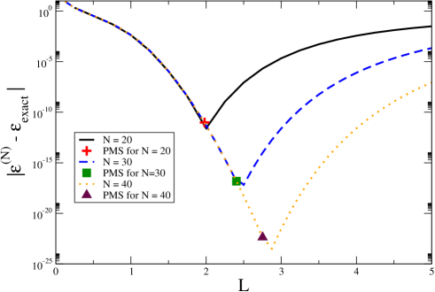
Figure 1: $|\varepsilon^{(N)}-\varepsilon_{exact}|$ for the RHO as a function of $L$ for $\mu=30$. The results of the PMS are also displayed. (color online)

We have used eq. (17) in the case of the RHO with $\mu=30$ and $\mu=5$, i.e. the case which was previously studied in the momentum representation. The numerical results that we have obtained in this nonlocal representation display a rate of convergence similar to the one observed in the local representation. In Fig. 1 we have plotted the difference $|\varepsilon^{(N)}-\varepsilon_{exact}|$ as a function of the scale $L$ and compared the results with the predictions obtained using the PMS condition eq. (18). Here $\varepsilon^{(N)}$ is the energy for the ground state obtained using a given value of $N$, whereas $\varepsilon_{exact}$ is approximated with the energy obtained using $N=100$.

In the case $\mu=5$ where the non-relativistic expansion provides a quite poor approximation with just a four digit precision, the result obtained in the non–local representation has $12$ correct digits for $N=50$: $(\varepsilon-\mu)=0.91531941208$.

Although the results obtained studying the RHO are sufficient in our opinion to prove the efficiency and simplicity of the method that we are proposing in this paper, we wish to consider few examples which can better illustrate the power of our method.

As a first example we have chosen the potential

$$V(x)=\sqrt{a^{2}+x^{2}}$$ (19)

and the corresponding SSE (with $x\in(0,\infty)$):

$$\left[\sqrt{\hat{p}^{2}+\mu^{2}}+\sqrt{a^{2}+x^{2}}\right]\ \psi(x)=\varepsilon\ \psi(x)\ .$$ (20)

Notice that for $a\gg 1$ and $\mu\gg 1$ one recovers the standard harmonic oscillator (SHO). We have applied our method using $a=\mu=1$ and we have obtained $(\varepsilon-\mu)=2.075870921$, using $N=100$, where all the displayed digits are correct.

As a second example that we wish to consider the SSE (with $x\in(0,\infty)$):

$$\left[\sqrt{\hat{p}^{4}+\hat{p}^{2}+\mu^{2}}+\sqrt{a^{2}+x^{2}}\right]\ \psi(x)=\varepsilon\ \psi(x)\ .$$ (21)

Also in this case we have assumed $\mu=a=1$ and we have obtained $(\varepsilon-\mu)=2.724199599$, using $N=100$, where all the displayed digits are correct.

As a final example we have considered the equation

$$\left\{\mu\ \log\left[1+\frac{\hat{p}^{2}}{2\mu^{2}}\right]+V(x)\right\}\psi(x)=E\ \psi(x)\ .$$ (22)

with $V(x)=x^{2}/2$ and $x\in(-\infty,+\infty)$. Notice that the equation obtained expanding to leading order in powers of $p/\mu$ is the standard Schrödinger equation for the harmonic oscillator. Despite the rather ugly form of the “kinetic” operator in the present case, the application of our method is straightforward and an expression for the matrix elements of the Hamiltonian is easily obtained:

$$H_{kj}=-\frac{\mu}{N}\sum_{n=-N}^{+N}(i)^{n+1}\ \sin\left(\frac{n\pi}{2}+\frac{kn\pi}{N}\right)\ \log\left\{1+\frac{n^{2}\pi^{2}}{8\mu^{2}L^{2}}\right\}\ e^{i\frac{jn\pi}{N}}+\delta_{kj}\ V(x_{k})\ .$$ (23)

We have solved this problem assuming $\mu=10$ and we have obtained the ground state energy $\varepsilon=20.04909725$ using $N=30$ (all the displayed digits are correct).

Although we did not have any physical model in mind when we considered the last two examples, we are aware that modifications of the standard Schrödinger equation (not necessarily of this kind) appear in several areas of research: for example, the introduction of a minimal length uncertainty relation naturally leads to modified Schrödinger equations (see for example Kempf95 ).

IV Green’s functions

In this Section we want to show that the method that we have developed in the previous Section can also be applied to the calculation of matrix elements of other non–local operators. We will see that SF and LSF are a powerful tool, and actually they have already been used earlier in a different context in applications to Quantum Field Theory (QFT) (see for example Gura00 ).

To start we consider an operator $\hat{O}\equiv f(\hat{p})$: in such case, the results that we have obtained in the previous Section apply straightforwardly and one obtains

$$O_{kj}=\frac{1}{N}\sum_{n=-N}^{+N}(i)^{n+1}\ \sin\left(\frac{n\pi}{2}+\frac{kn\pi}{N}\right)\ f\left(i\frac{n\pi}{2L}\right)\ \ e^{i\frac{jn\pi}{N}}\ .$$ (24)

One example of application of this formula is the calculation of the Green’s function for a free particle in a box, $|x|<L$, which is given by (see for example Feynman ; Schulman )

$$G^{(0)}(y,0;x,t) = \langle x|e^{-i\frac{\hat{p}^{2}}{2\mu}t}|y\rangle\ .$$

The notation $|x\rangle$ indicates a state localized at a point $x$: in our formalism this is simply represented by a SF or a LSF with a peak at this point. Notice however that SF and LSF are not normalized to one, see Amore06a ; Amore06b , which means that we have an extra factor $1/\sqrt{h}\equiv\sqrt{N/2L}$ for each SF or LSF, where $h$ is the spacing of the grid.

Therefore we can write:

$$G^{(0)}(x_{j},0;x_{k},t) = -\frac{1}{Nh}\sum_{n=-N}^{+N}(i)^{n+1}\ \sin\left(\frac{n\pi}{2}+\frac{kn\pi}{N}\right)\ e^{-it\left[\frac{1}{2\mu}\left(\frac{n\pi}{2L}\right)^{2}\right]}\ e^{i\frac{jn\pi}{N}}\ ,$$ (25)

$x_{k}$ and $x_{j}$ being points on the grid. In the limit of an infinitely dense grid one can switch from the discrete indices $k,j$ to the continuum indices $x,y$:

$$G^{(0)}(y,0;x,t) = -\frac{1}{2L}\ \sum_{n=-N}^{+N}i^{n+1}e^{\frac{in\pi x}{2L}-\frac{in^{2}\pi^{2}t}{8L^{2}\mu}}\ \sin\left(\frac{\pi yn}{2L}+\frac{\pi n}{2}\right)$$ (26)

Notice that in the case of a free particle the exact result can be calculated with the standard path integral and reads

$$G^{(0)}(0,0;x,t)=\sqrt{\frac{\mu}{2\pi it}}\ e^{i\frac{\mu x^{2}}{2t}}\ .$$ (27)

In our formalism we have

$$G^{(0)}(0,0;x,t) = -\frac{1}{2L}\ \sum_{n=-N}^{+N}i^{n+1}e^{\frac{in\pi x}{2L}-\frac{in^{2}\pi^{2}t}{8L^{2}\mu}}\ \sin\left(\frac{\pi n}{2}\right)$$ (28)

$$= \frac{1}{2L}\sum_{n=-N/2}^{+N/2}\ e^{-\frac{i\pi^{2}tn^{2}}{2L^{2}\mu}-\frac{i\pi^{2}tn}{2L^{2}\mu\ }+\frac{i\pi xn}{L}-\frac{i\pi^{2}t}{8L^{2}\mu}+\frac{i\pi x}{2L}}$$ (29)

For $N\gg 1$ we can approximate this sum with an integral and thus obtain which reads

$$G^{(0)}(0,0;x,t) = \frac{1}{2}\ \sqrt{\frac{\mu}{2\pi it}}\ e^{i\frac{\mu x^{2}}{2t}}\left[\text{Erf}\left(\frac{\left(\frac{1}{4}+\frac{i}{4}\right)((N+1)\pi t-2L\ \mu x)}{L\sqrt{\mu t}}\right)+\text{Erf}\left(\frac{\left(\frac{1}{4}+\frac{i}{4}\right)\ ((N-1)\pi t+2L\mu x)}{L\sqrt{\mu t}}\right)\right]\ .$$ (30)

In the limit $N\rightarrow\infty$ we can approximate each error function to one and therefore obtain the exact expression (27).

To further test this formula we can also use the Feynman-Kac formula to extract the ground state energy

$$E_{0}=-\lim_{\tau\rightarrow\infty}\frac{1}{\tau}\log\int dx\ G(x,-i\tau,x,0)\ .$$ (31)

In our case the integral appearing in (31) becomes a sum over all the grid points and therefore reads

$$E_{0}=-\lim_{\tau\rightarrow\infty}\frac{1}{\tau}\log\left\{\frac{1}{Nh}\sum_{k=-N/2+1}^{N/2-1}\sum_{n=-N}^{+N}(i)^{n+1}\ \sin\left(\frac{n\pi}{2}+\frac{kn\pi}{N}\right)\ e^{-\tau\left[\frac{1}{2\mu}\left(\frac{n\pi}{2L}\right)^{2}\right]}\ e^{i\frac{kn\pi}{N}}\right\}.$$ (32)

Because we are taking the limit $\tau\rightarrow\infty$, the exponential factor in this expression will be quite small unless $n=\pm 1$ (the term $n=0$ vanishes). For this reason we can approximate

$$E_{0} = -\lim_{\tau\rightarrow\infty}\frac{1}{\tau}\log\left\{\frac{1}{Nh}\sum_{k=-N/2+1}^{N/2-1}\left[2e^{-\frac{\pi^{2}\tau}{8\mu L^{2}}}\cos^{2}\left(\frac{k\pi}{N}\right)\right]\right\}$$ (33)

$$= -\lim_{\tau\rightarrow\infty}\frac{1}{\tau}\log\left\{e^{-\frac{\pi^{2}\tau}{8\mu L^{2}}}\right\}=\frac{\pi^{2}}{8\mu L^{2}}$$

which is indeed the exact ground state of the particle in the box.

We can now consider the more general case in which the Hamiltonian contains a potential. In this case the formula of Section IV cannot be applied directly because $\hat{p}$ and $\hat{x}$ do not commute. However we can use the Trotter product formula to write Feynman ; Schulman

$$G(y,0;x,t) = \lim_{\bar{N}\rightarrow\infty}\langle x|\left(e^{-i\frac{\hat{p}^{2}}{2\mu\bar{N}}t}e^{-i\frac{V}{\bar{N}}t}\right)^{\bar{N}}|y\rangle\ .$$ (34)

We can use the completeness of the coordinate states, $|x\rangle$, to write

$$G(y,0;x,t) = \lim_{\bar{N}\rightarrow\infty}\sum_{r_{1},r_{2},\dots,r_{\bar{N}}}\langle x|\left(e^{-i\frac{\hat{p}^{2}}{2\mu\bar{N}}t}e^{-i\frac{V}{\bar{N}}t}\right)|x_{r_{1}}\rangle\langle x_{r_{1}}|\left(e^{-i\frac{\hat{p}^{2}}{2\mu\bar{N}}t}e^{-i\frac{V}{\bar{N}}t}\right)|x_{r_{2}}\rangle\dots\langle x_{r_{\bar{N}}}|\left(e^{-i\frac{\hat{p}^{2}}{2\mu\bar{N}}t}e^{-i\frac{V}{\bar{N}}t}\right)|y\rangle\ ,$$ (35)

where the indices $r_{i}$ span all the lattice. Notice the factors $t/\bar{N}$, which correspond to having a “time–slicing”, as usual in path integration; at each intermediate time each point on the grid can be reached.

We define

$${\cal V}_{\bar{N}}(x_{i},t)\equiv h\ \langle x_{i}|e^{-i\frac{V(x)}{\bar{N}}t}|x_{j}\rangle=e^{-i\frac{V(x_{i})}{\bar{N}}t}\delta_{ij}\ ,$$ (36)

which is diagonal in the coordinates. We can now write the compact expression

$$G(y,0;x,t) = \lim_{\bar{N}\rightarrow\infty}\frac{1}{h^{\bar{N}}}\ \sum_{r_{1},r_{2},\dots,r_{\bar{N}}}G^{(0)}(x_{r_{1}},t-\varepsilon;x,t)\ {\cal V}_{\bar{N}}(x_{r_{1}},t)\ G^{(0)}(x_{r_{2}},t-2\varepsilon;x_{r_{1}},t-\varepsilon)$$ (37)

$${\cal V}_{\bar{N}}(x_{r_{2}},t)\ \dots\ {\cal V}_{\bar{N}}(x_{r_{\bar{N}}},t)\ G^{(0)}(y,0;x_{r_{\bar{N}}},\varepsilon)\ ,$$

where $\varepsilon\equiv t/\bar{N}$. This expression should be compared with the standard path integral expressionFeynman ; Schulman

$$G(x,t;y,0) = \lim_{N\rightarrow\infty}\ \int dx_{1}\dots dx_{N-1}\ \left(\frac{\mu}{2\pi i\epsilon}\right)^{N/2}\ e^{i\epsilon\sum_{j=0}^{N-1}\left[\frac{\mu}{2}\left(\frac{x_{j+1}-x_{j}}{\epsilon}\right)^{2}-V(x_{j})\right]}\ ,$$ (38)

where $\epsilon\equiv t/N$.

Our equation (37) can be also compared with the exact expressions for the $N$-fold time sliced spacetime propagators which Crandall has obtained in eqs.(2.9) and (2.12) of Crandall93 using the standard representation.

Our result of eq. (37) provides a new representation of the path integral for quantum mechanical problems with a clear physical interpretation: the propagation of a particle sitting at $y$ at time $t=0$ and reaching $x$ at time $t$ occurs moving at each time interval, $\varepsilon$, from a point of the grid to another one in all possible ways (remember the sums over the grid points). $G^{(0)}(x_{i},t;x_{j},t+\varepsilon)$ represents the probability of going from a point $x_{i}$ to another point $x_{j}$ on the grid in a time interval $\varepsilon$; at this point an interaction take place, through the the potential term ${\cal V}$. We stress that our representation corresponds to a different way of discretizing space which also allows to deal with Hamiltonians containing non–local operators (the SSE is one example) and could be an useful tool for problems which cannot be easily treated with the conventional formalism.

V Conclusions

In this paper we have derived an analytical expression for the non–local relativistic kinetic energy operator which appears in the Salpeter equation. This representation is exact in the limit of an arbitrarily fine grid and we have used it to solve the Salpeter equation for the Relativistic Harmonic Oscillator, where semi–analytical results are available. We have found that our representation can be used together with the Variational Sinc Collocation Method (VSCM) to provide arbitrarily precise results, with a strong rate of convergence. The most important result of this paper is the new representation for the quantum mechanical Green’s function, which requires the evaluation of matrix elements of non–local operators. We have provided a general formula and we have explicitly tested it in the case of a free particle in a box, recovering the exact result. Our new representation of the path integral can be applied also to problems in which the Hamiltonian contains non–local operators (which would be the case of the Salpeter equation) and it is suitable both for numerical and analytical calculations, in the cases in which the limits $N,\bar{N}\rightarrow\infty$ can be calculated (as for a free particle in a box).

Given the importance of path integrals in many areas of Physics, we feel that the results contained in this paper could have a large number of applications. Finally, we wish to mention that it would be worth exploring the possibility to use the PMS in a numerical scheme to optimize convergence to the exact result for finite values of $N$ and $\bar{N}$. It also remains to explore the possibility to apply our formalism to Quantum Field Theory (QFT), which we plan to address in future works.

References

- (1) L.J.Nickisch, L.Durand and B.Durand, Phys. Rev. D30, 660 (1984)
- (2) C. Long, Phys. Rev. D 30, 1970 (1984)
- (3) W. Lucha, H. Rupprecht and F.F. Schöberl, Phys. Rev. D 45, 1233-1239 (1992)
- (4) L.P. Fulcher, Phys. Rev. D 50, 447 (1994)
- (5) J.W. Norbury, K. Maung Maung and D. E. Kahana, Phys. Rev. D 50, 3609 (1994)
- (6) C. Semay, D. Baye, M. Hesse and B. Silvestre-Brac, Phys. Rev.E 64, 016703 (2005)
- (7) P. Amore, A variational sinc collocation method for strong coupling problems, Journal of Physics A 39, L349-L355 (2006)
- (8) P. Amore, M. Cervantes and F.M. Fernández, ArXiv:[quant-ph/0608069] (2006)
- (9) W. Lucha and F.F. Schöberl, Phys. Rev. A 54, 3790-3794 (1996)
- (10) W. Lucha and F.F. Schöberl, J. Math. Phys.41, 1778 (2000)
- (11) R. Hall, W. Lucha and F.F. Schöberl, J. Phys. A 34, 5059-5063 (2001)
- (12) R. Hall and W. Lucha, J. Phys. A 38, 7977-8002 (2005)
- (13) W. Lucha and F.F. Schöberl, Phys. Rev. A 51, 4419- 4426 (1995)
- (14) M.Znojil, J. of Phys. A 29, 2905 (1996)
- (15) O. Mustafa and M. Odeh, J. of Phys. A 32, 6653 (1999)
- (16) Li, Liu, W. Lucha, Ma and F.F. Schöberl, J. Math. Phys.46, 103514 (2005)
- (17) C. Schwartz, Journal of Mathematical Physics 26, 411-415 (1985)
- (18) D. Baye, Journal of Physics B 28, 4399-4412 (1995)
- (19) M. Trott, The Mathematica guidebook for symbolics, Springer
- (20) P. Amore, A. Aranda, F.M. Fernández and H.F. Jones, Physics Letters A 340, 87-93 (2005)
- (21) P. M. Stevenson, Phys. Rev. D 23, 2916 (1981).
- (22) A. Kempf, G.Mangano and R.B. Mann, Phys. Rev. D 52 1108 (1995)
- (23) R. Easther, G.Guralnik and S.Hahn, Phys. Rev. D 61, 125001 (2000)
- (24) R.P.Feynman and A.R.Hibbs, Quantum mechanics and path integrals, McGraw-Hill, New York (1965)
- (25) L.S. Schulman, Techniques and applications of Path Integration, John Wiley and Sons, New York (1981)
- (26) R.E. Crandall, J. Phys. A 26, 3627-3648 (1993)