KUNS-2058

hep-th/0701031

January 2007

abstract

We study $(p,q)=(2,4k)$ minimal superstrings within the minimal superstring field theory constructed in hep-th/0611045. We explicitly give a solution to the $W_{1+\infty}$ constraints by using charged D-instanton operators, and show that the $(m,n)$-instanton sector with $m$ positive-charged and $n$ negative-charged ZZ-branes is described by an $(m+n)\times(m+n)$ supermatrix model. We argue that the supermatrix model can be regarded as an open string field theory on the multi ZZ-brane system.

1 Introduction

Minimal noncritical (super)string theories [1, 2, 3, 4] are good toy models for investigating various aspects of string theory. They have fewer degrees of freedom but still share many features with their critical-string counterparts. Furthermore, there exists a string field theory [5, 6, 7, 8, 9, 10] which can completely describe both of fundamental strings (FZZT branes) and D-branes (D-instantons, ZZ branes), and has a clear relationship with Liouville-theory analysis [11, 12, 13, 14, 15, 16, 17, 18]. In particular, in [10] the spacetime which noncritical superstrings describe is clarified in terms of the two-component KP hierarchy.

The aim of this letter is to further study the structure of spacetime in minimal superstring theories, especially the one emerging from 2-cut one-matrix models [19, 20, 21, 22, 23, 24, 25, 26, 27]. We show that spacetime probed by ZZ-branes has a description in terms of supermatrix models.

This letter is organized as follows. In section 2, we make a brief review on type 0 minimal superstring theory and its string-field formulation [10]. In section 3, we explicitly give a solution to the $W_{1+\infty}$ constraints in the case of $\hat{p}=1$ minimal superstring theory, and show that the partition function of the $(m,n)$-instanton sector with $m$ positive-charged and $n$ negative-charged ZZ-branes has a simple integral representation. In section 4, we show that the partition function of the $(m,n)$-instanton sector is expressed as an $(m+n)\times(m+n)$ hermitian supermatrix model, which can be interpreted as an open string field theory on the multi ZZ-brane system. Section 5 is devoted to discussions.

2 Minimal superstring field theory

Minimal type 0 superstring theory describes a product of minimal superconformal field theory (SCFT) and super Liouville field theory. Minimal SCFTs are characterized by the central charges $\hat{c}^{\rm(matter)}(p,q)=1-2(q-p)^{2}/qp$ and are classified into two classes [28]:

• even minimal SCFT: $(p,q)=(2\hat{p},2\hat{q})$ with $\hat{p}+\hat{q}\in 2\mathbb{Z}+1$

• odd minimal SCFT:   $(p,q)=(\hat{p},\hat{q})$      with $\hat{p},\,\hat{q}$: odd

The scaling operators $\sigma^{[\mu]\,{\rm(matter)}}_{n}(z,\bar{z})$ belonging to $(p,q)$ SCFT have conformal dimensions

$$\Delta_{n}^{[\mu]\,{\rm(matter)}}=\bar{\Delta}_{n}^{[\mu]\,{\rm(matter)}}=\frac{n^{2}-(\hat{q}-\hat{p})^{2}}{8\hat{q}\hat{p}}+\frac{\mu}{16}\quad\Bigl{(}n\geq 1;~{}\mu=0\,(\mbox{NS-NS})~{}\mbox{or}~{}1\,(\mbox{R-R})\Bigr{)}\,,$$ (2.1)

where $n$ and $\mu$ correspond to $(r,s)$ in the Kac table as $n=\hat{q}r-\hat{p}s$ and $\mu=r-s~{}(\mbox{mod}\,2)$. They are dressed with super Liouville field [3] to become

$$\mathcal{O}^{[\mu]}_{n}=\int\!d^{2}z\,\sigma^{[\mu]\,{\rm(matter)}}_{n}(z,\bar{z})\,\sigma^{[\mu]\,{\rm(Liouville)}}_{n}(z,\bar{z})\qquad(n\geq 1;~{}\mu=0,1).$$ (2.2)

The partition function with R-R background flux $\nu$

$$\tau_{\nu}(x)\equiv\left\langle\exp\Bigl{[}(1/g)\sum_{n\geq 1}\bigl{(}x^{[0]}_{n}\mathcal{O}^{[0]}_{n}+x^{[1]}_{n}\mathcal{O}^{[1]}_{n}\bigr{)}\Bigr{]}\right\rangle_{\!\!\!\nu}$$ (2.3)

is given by a $\tau$ function of two-component KP (2cKP) hierarchy [10]. To explain this, we make a few preparations (see [10] for further explanations).

First we introduce two sets of chiral fermions on complex $\lambda$ plane,

$$\psi^{(i)}(\lambda)=\sum_{r\in\mathbb{Z}+1/2}\psi^{(i)}_{r}\lambda^{-r-1/2},\quad\bar{\psi}^{(i)}(\lambda)=\sum_{r\in\mathbb{Z}+1/2}\bar{\psi}^{(i)}_{r}\lambda^{-r-1/2}\quad(i=1,2)\,,$$ (2.4)

$$\bigl{\{}\psi^{(i)}_{r},\psi^{(j)}_{s}\bigr{\}}=\delta^{ij}\,\delta_{r+s,0}\,,$$ (2.5)

with the Dirac vacuum $\bigl{|}0\bigr{>}$, $\psi^{(i)}_{r}\,\bigl{|}0\bigr{>}=\bar{\psi}^{(i)}_{r}\,\bigl{|}0\bigr{>}=0$ $(r>0)$. We bosonize them as $\psi^{(i)}(\lambda)=e^{\phi^{(i)}(\lambda)}$, $\bar{\psi}^{(i)}(\lambda)=e^{-\phi^{(i)}(\lambda)}$ $(i=1,2)$ with

$$\phi^{(i)}(\lambda)=q^{(i)}+\alpha^{(i)}_{0}\,\ln\lambda-\sum_{n\neq 0}\,\frac{\alpha^{(i)}_{n}}{n}\,\lambda^{-n},\qquad\bigl{[}\alpha^{(i)}_{m},\alpha^{(j)}_{n}\bigr{]}=m\,\delta^{ij}\,\delta_{m+n,0}.$$ (2.6)

The state $\bigl{|}\nu\bigr{>}\equiv e^{\nu\,\bigl{(}q^{(1)}-q^{(2)}\bigr{)}}\,\bigl{|}0\bigr{>}$ then describes the asymptotic state where the Fermi levels of the first $(i=1)$ and the second $(i=2)$ fermions differ by $2\nu$. This degree of freedom, $\nu$, can actually be interpreted as background R-R flux in the weak coupling region [26, 27].

We then introduce twisted bosons and twisted fermions on $\zeta\equiv\lambda^{\hat{p}}$ plane as

$$\varphi^{(i)}_{0}(\zeta)\equiv\phi^{(i)}(\lambda)~{}~{}\Rightarrow~{}~{}\varphi^{(i)}_{a}(\zeta)\equiv\varphi^{(i)}_{0}(e^{2\pi ia}\zeta),$$

$$c^{(i)}_{a}(\zeta)\equiv e^{\varphi^{(i)}_{a}(\zeta)},\quad\bar{c}^{(i)}_{a}(\zeta)\equiv e^{-\varphi^{(i)}_{a}(\zeta)}\quad(i=1,2;~{}a=0,1,\cdots,\hat{p}-1)\,,$$ (2.7)

from which the $W_{1+\infty}$ currents [29] are defined as

$$W^{s}(\zeta) \equiv\sum_{n\in\mathbb{Z}}W_{n}^{s}\zeta^{-n-s}$$

$$=s\,\sum_{a=0}^{\hat{p}-1}\,\Bigl{(}:\!\partial^{s-1}c^{(1)}_{a}(\zeta)\cdot\bar{c}_{a}^{(1)}(\zeta)\!:+(-1)^{s}\Bigl{[}:\!\partial^{s-1}c^{(2)}_{a}(\zeta)\cdot\bar{c}_{a}^{(2)}(\zeta)\!:\Bigr{]}_{\zeta\to-\zeta}\Bigr{)}$$

$$=\sum_{a=0}^{\hat{p}-1}\,\bigl{(}:e^{-\varphi^{(1)}_{a}(\zeta)}\partial^{s}\,e^{\varphi^{(1)}_{a}(\zeta)}:+:e^{-\varphi^{(2)}_{a}(-\zeta)}\partial^{s}\,e^{\varphi^{(2)}_{a}(-\zeta)}:\bigr{)}.$$ (2.8)

The normal ordering $:\,\,:$ is taken with the ${\rm SL}(2,\mathbb{C})$ invariant vacuum on $\zeta$ plane, so that the monodromy like $\varphi^{(i)}_{a}(e^{2\pi i}\zeta)=\varphi^{(i)}_{a+1}(\zeta)$ should be interpreted as a relation to hold in correlation functions where $\mathbb{Z}_{\hat{p}}$-twist fields are inserted at $\zeta=0$ and $\zeta=\infty$.

By introducing

$$\alpha^{[\mu]}_{n}\equiv\alpha^{(1)}_{n}+(-1)^{\mu}\,\alpha^{(2)}_{n}\,,\quad x^{[\mu]}_{n}\equiv\frac{1}{2}\,\bigl{(}x^{(1)}_{n}+(-1)^{\mu}x^{[\mu]}_{n}\bigr{)}\quad(\mu=0,1),$$ (2.9)

the partition function is expressed as

$$\tau_{\nu}(x) =\bigl{<}\nu\,\bigr{|}\,e^{(1/g)\sum_{n\geq 1}\bigl{(}x^{[0]}_{n}\alpha^{[0]}_{n}+x^{[1]}_{n}\alpha^{[1]}_{n}\bigr{)}}\bigl{|}\Phi\bigr{>}=\bigl{<}\nu\,\bigr{|}\,e^{(1/g)\sum_{n\geq 1}\bigl{(}x^{(1)}_{n}\alpha^{(1)}_{n}+x^{(2)}_{n}\alpha^{(2)}_{n}\bigr{)}}\bigl{|}\Phi\bigr{>}$$

$$\equiv\bigl{<}x/g;\nu\,\bigr{|}\Phi\bigr{>},$$ (2.10)

where the state $\bigl{|}\Phi\bigr{>}$ satisfies the following two conditions [10]:

$$\begin{array}[]{l}\bullet\,\,\mbox{\text@underline{decomposability}; ~{}$\bigl{|}\Phi\bigr{>}$ is written in the form $e^{\rm(fermion~{}bilinear)}\,\bigl{|}0\bigr{>}$}\\ \bullet\,\,\mbox{\text@underline{$W_{1+\infty}$ constraints};\, $W^{s}_{n}\,\bigl{|}\Phi\bigr{>}=0$ ($s\geq 1;\,n\geq-s+1$)}\end{array}$$ (2.13)

as in the bosonic case [30, 31, 32, 33, 34, 35, 36, 37]. The first condition is equivalent to the statement that $\tau_{\nu}(x)$ is a $\tau$ function of 2cKP hierarchy [38, 39, 40, 41, 42]. The second one represents the whole set of the Schwinger-Dyson equations [32, 33, 35, 36, 37]. In the language of two-cut matrix models with symmetric double-well potentials, $\alpha^{[0]}_{n}$ (resp. $\alpha^{[1]}_{n}$) describe symmetric (resp. antisymmetric) fluctuations of eigenvalues [43, 44, 26], so that $\alpha^{(1)}_{n}$ and $\alpha^{(2)}_{n}$ describe fluctuations in the right and the left well, respectively.

According to our ansatz on operator identification [10], the excitations in the NS-NS and R-R sectors are collected into:

$$\mbox{\text@underline{NS-NS scalar}}: \quad\partial\varphi^{[0]}_{0}(\zeta)=\partial\varphi^{(1)}_{0}(\zeta)+\partial\varphi^{(2)}_{0}(\zeta)=\frac{1}{\hat{p}}\,\sum_{n\in\mathbb{Z}}\,\alpha^{[0]}_{n}\,\zeta^{-n/\hat{p}-1},$$ (2.14)

$$\mbox{\text@underline{R-R scalar}}: \quad\partial\varphi^{[1]}_{0}(\zeta)=\partial\varphi^{(1)}_{0}(\zeta)-\partial\varphi^{(2)}_{0}(\zeta)=\frac{1}{\hat{p}}\,\sum_{n\in\mathbb{Z}}\,\alpha^{[1]}_{n}\,\zeta^{-n/\hat{p}-1}.$$ (2.15)

Their connected correlation functions (or cumulants) in the presence of background R-R flux $\nu$ are given by

$$\left\langle\partial\varphi_{0}^{(i_{1})}(\zeta_{1})\cdots\partial\varphi_{0}^{(i_{N})}(\zeta_{N})\right\rangle_{\!\nu,{\rm c}} =\biggl{[}\frac{\bigl{<}x/g;\nu\,\bigr{|}:\!\partial\varphi^{(i_{1})}_{0}(\zeta_{1})\cdots\partial\varphi^{(i_{N})}_{0}(\zeta_{N})\!:\bigl{|}\Phi\bigr{>}}{\bigl{<}x/g;\nu\,\bigr{|}\,\Phi\bigr{>}}\biggr{]}_{\rm c}$$

$$=\sum_{h\geq 0}\,g^{2h+N-2}\,\left\langle\,\partial\varphi^{(i_{1})}_{0}(\zeta_{1})\cdots\partial\varphi^{(i_{N})}_{0}(\zeta_{N})\,\right\rangle^{\!(h)}_{\!\nu,{\rm c}}.$$ (2.16)

Comparing the disk amplitudes with the algebraic curves of FZZT branes in super Liouville theory, we find the correspondence [10]:

$$\mbox{\text@underline{boundary states}}:\qquad\bigl{|}{\rm\,FZZT}+;+\zeta\bigr{>}\Leftrightarrow\varphi_{0}^{(1)}(\zeta),\quad\bigl{|}{\rm\,FZZT}-;-\zeta\bigr{>}\Leftrightarrow\varphi_{0}^{(2)}(-\zeta)\,.$$ (2.17)

Once a charged FZZT brane is located at a point in spacetime with coordinate $\zeta_{\rm bos}=\zeta^{2}$ [10], it becomes a source of fundamental strings, with a bunch of worldsheets which are not connected with each other in the sense of worldsheet topology, but are connected in spacetime with their boundaries pinched at the same superspace point $\zeta$. These configurations are easily summed up to give an exponential form as in the bosonic case [7], realizing the spacetime combinatorics of Polchinski [45]:

$$\mbox{\text@underline{charged FZZT branes}}:\quad c^{(1)}_{a}(\zeta)=e^{\varphi^{(1)}_{a}(\zeta)},\quad c^{(2)}_{a}(-\zeta)=e^{\varphi^{(2)}_{a}(-\zeta)}\quad(a=0,1,\cdots,\hat{p}-1)\,.$$ (2.18)

As in the bosonic case [5], the D-instanton operators [10]

$$D_{ab}^{(ij)}=\oint\bigcirc\frac{d\zeta}{2\pi i}\,c_{a}^{(i)}(\zeta^{(i)})\bar{c}_{b}^{(j)}(\zeta^{(j)})=\oint\bigcirc\frac{d\zeta}{2\pi i}\,:\!e^{\varphi^{(i)}_{a}(\zeta^{(i)})-\varphi^{(j)}_{b}(\zeta^{(j)})}\!:$$

$$\bigl{(}\mbox{$i=j$ with $a\neq b$; $i\neq j$ with $\forall(a,b)$};~{}\zeta^{(1)}\equiv+\zeta,\,\zeta^{(2)}\equiv-\zeta\bigr{)}$$ (2.19)

commute with the $W_{1+\infty}$ generators:

$$\bigl{[}W^{s}_{n},\,D_{ab}^{(ij)}\bigr{]}=0,$$ (2.20)

where the contour of (2.19) surrounds $\zeta=\infty$ $\hat{p}$ times to resolve the monodromy of $\zeta$ plane. Equation (2.20) implies that given a state $\bigl{|}\Phi\bigr{>}$ satisfying the $W_{1+\infty}$ constraints, one can construct another such state by multiplying it with $D^{(ij)}_{ab}$’s. By further requiring that the resulting state be decomposable $\bigl{(}$ i.e. can be written as $e^{{\rm(fermion~{}bilinear)}}\,\bigl{|}0\bigr{>}\,\bigr{)}$, the product of D-instanton operators must be accumulated to have the following form with fugacity $\theta^{(ij)}_{ab}$ [6]:

$$\bigl{|}\Phi;\theta\bigr{>}\equiv\prod_{i,j}\prod_{a,b}\,\exp\Bigl{[}\theta^{(ij)}_{ab}\,D^{(ij)}_{ab}\Bigr{]}\,\bigl{|}\Phi\bigr{>}.$$ (2.21)

Note that $D^{(ij)}_{ab}$ $(i\neq j)$ includes the operator $e^{q^{(i)}-q^{(j)}}$ and thus changes the relative Fermi levels. We thus have the following two classes of D-instanton operators:

neutral D-instanton operators $(a\neq b)$:

$$D_{ab}^{(11)} =\oint\bigcirc\frac{d\zeta}{2\pi i}\,c_{a}^{(1)}(\zeta)\,\bar{c}_{b}^{(1)}(\zeta)=\oint\bigcirc\frac{d\zeta}{2\pi i}\,:\!e^{\varphi^{(1)}_{a}(\zeta)-\varphi^{(1)}_{b}(\zeta)}\!:\,,$$

$$D_{ab}^{(22)} =\oint\bigcirc\frac{d\zeta}{2\pi i}\,c_{a}^{(2)}(-\zeta)\,\bar{c}_{b}^{(2)}(-\zeta)=\oint\bigcirc\frac{d\zeta}{2\pi i}\,:\!e^{\varphi^{(2)}_{a}(-\zeta)-\varphi^{(2)}_{b}(-\zeta)}\!:.$$ (2.22)

charged D-instanton operators $(\forall a,\forall b)$:

$$D_{ab}^{(12)} =\oint\bigcirc\frac{d\zeta}{2\pi i}\,c_{a}^{(1)}(\zeta)\,\bar{c}_{b}^{(2)}(-\zeta)=\oint\bigcirc\frac{d\zeta}{2\pi i}\,:\!e^{\varphi^{(1)}_{a}(\zeta)-\varphi^{(2)}_{b}(-\zeta)}\!:\,,$$

$$D_{ab}^{(21)} =\oint\bigcirc\frac{d\zeta}{2\pi i}\,c_{a}^{(2)}(-\zeta)\,\bar{c}_{b}^{(1)}(\zeta)=\oint\bigcirc\frac{d\zeta}{2\pi i}\,:\!e^{\varphi^{(2)}_{a}(-\zeta)-\varphi^{(1)}_{b}(\zeta)}\!:.$$ (2.23)

In the weak coupling limit, $g\to+0$, one D-instanton amplitude $\bigl{<}D^{(ij)}_{ab}\bigr{>}$ can be evaluated by the saddle points $\zeta=\zeta_{*}$ of the exponent $\Gamma^{(ij)}_{ab}(\zeta)\equiv\bigl{<}\varphi^{(i)}_{a}(\zeta^{(i)})\bigr{>}^{\!\!(h=0)}-\bigl{<}\varphi^{(j)}_{b}(\zeta^{(j)})\bigr{>}^{\!\!(h=0)}$ as $\bigl{<}D^{(ij)}_{ab}\bigr{>}\sim e^{(1/g)\,\Gamma^{(ij)}_{ab}(\zeta_{*})}$ [8, 9, 10]. This gives the relation between the amplitudes of the ZZ-branes and those of the FZZT-branes [15] (see [10] for a detailed analysis).

3 $\hat{p}=1$ minimal superstrings

A great simplification occurs when $\hat{p}=1$, because $\zeta=\lambda$ in this case and the Dirac vacuum $\bigl{|}0\bigr{>}$ gives a trivial solution to the $W_{1+\infty}$ constraints. The general solutions are then given by

$$\bigl{|}\Phi;\,\theta_{+},\theta_{-}\bigr{>}=e^{\theta_{+}D_{+}}e^{\theta_{-}D_{-}}\,\bigl{|}0\bigr{>},$$ (3.1)

where $D_{+}\equiv D_{00}^{(12)}$, $D_{-}\equiv D_{00}^{(21)}$, and $\theta_{+}\equiv\theta_{00}^{(12)}$, $\theta_{-}\equiv\theta_{00}^{(21)}$. One can easily see that these states actually satisfy both of the conditions (2.13). The fugacities $\theta_{\pm}$ represent the moduli of solutions. Note that there are no neutral ZZ-branes when $\hat{p}=1$.

The ground canonical partition function is expanded as

$$\tau_{\nu}(x)=\bigl{<}x/g;\nu\,\bigr{|}\,\Phi;\theta_{+},\theta_{-}\bigr{>}=\sum_{m,\,n;\,\,m-n=\nu}\,\frac{\theta_{+}^{m}\,\theta_{-}^{n}}{m!\,n!}\,\,Z_{m,n}(x),$$ (3.2)

where

$$Z_{m,n}(x) =\bigl{<}x/g;\nu=m-n\bigr{|}\,D_{+}^{m}\,D_{-}^{n}\,\bigl{|}0\bigr{>}$$

$$=\oint\bigcirc\prod_{r=1}^{m}\frac{d\zeta^{+}_{r}}{2\pi i}\,\prod_{\alpha=1}^{n}\frac{d\zeta^{-}_{\alpha}}{2\pi i}\cdot(-1)^{(n+m)(n+m-1)/2}\,\times$$

$$\qquad\times\bigl{<}x/g;\nu=m-n\,\bigr{|}\,\prod_{r=1}^{m}:\!e^{\varphi^{(1)}_{0}(\zeta^{+}_{r})-\varphi^{(2)}_{0}(-\zeta^{+}_{r})}\!:\prod_{\alpha=1}^{n}:\!e^{\varphi^{(2)}_{0}(-\zeta^{-}_{\alpha})-\varphi^{(1)}_{0}(\zeta^{-}_{\alpha})}\!:\bigl{|}0\bigr{>}$$

is the partition function of the $(m,n)$-instanton sector with $m$ positive-charged and $n$ negative-charged ZZ-branes. This can be rewritten as

$$Z_{m,n}(x) =\bigl{<}x/g;\nu=m-n\,\bigr{|}\,D_{+}^{m}\,D_{-}^{n}\,\bigl{|}0\bigr{>}$$

$$=\oint\bigcirc\prod_{r=1}^{m}\frac{d\zeta^{+}_{r}}{2\pi i}\,\prod_{\alpha=1}^{n}\frac{d\zeta^{-}_{\alpha}}{2\pi i}\,\,\dfrac{\displaystyle\prod_{r<s}\bigl{(}\zeta^{+}_{r}-\zeta^{+}_{s}\bigr{)}^{2}\,\prod_{\alpha<\beta}\bigl{(}\zeta^{-}_{\alpha}-\zeta^{-}_{\beta}\bigr{)}^{2}}{\displaystyle\prod_{r}\prod_{\alpha}\bigl{(}\zeta^{+}_{r}-\zeta^{-}_{\alpha}\bigr{)}^{2}}\,\cdot\,e^{(1/g)\bigl{[}\sum_{r}\Gamma(\zeta^{+}_{r})\,-\,\sum_{\alpha}\Gamma(\zeta^{-}_{\alpha})\bigr{]}},$$ (3.4)

where the D-instanton action $\Gamma(\zeta)$ is given by

$$\Gamma(\zeta)=\sum_{n=1}^{1+\hat{q}}(x_{n}^{(1)}+(-1)^{n+1}x_{n}^{(2)})\zeta^{n}\equiv\sum_{n=1}^{1+\hat{q}}x_{n}\zeta^{n}.$$ (3.5)

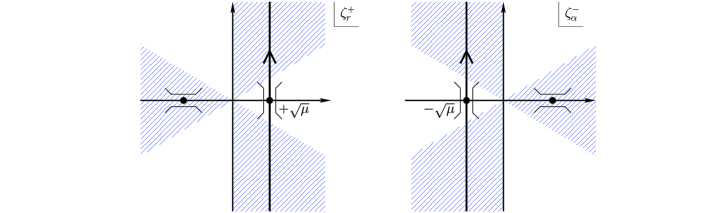
Figure 1: Contours of $\zeta^{+}_{r}$ and $\zeta^{-}_{\alpha}$ for pure supergravity, $(p,q)=(2,4)$. The blobs are the saddle points of the functions $\Gamma(\zeta^{+}_{r})$ and $\Gamma(\zeta^{-}_{\alpha})$, and the accompanying bridges show their associated steepest descent directions. The shaded regions are the Stokes sectors where the real parts of the functions become negative for $|\zeta_{r}^{+}|,\,|\zeta_{\alpha}^{-}|\to\infty$.

The contours are chosen such that the state (3.1) is defined well for some region in the parameter space of backgrounds, $\bigl{\{}x^{(i)}_{n}\bigr{\}}$. In the case of pure supergravity, $(p,q)=(2,4)$ (or $(\hat{p},\hat{q})=(1,2)$), for example, one can take the contour as in fig. 1 if we take a background as $x^{(1)}_{3}=x^{(2)}_{3}=1/3$ and $x^{(1)}_{1}=x^{(2)}_{1}=-\mu$. In fact, this background leads to $\Gamma(\zeta)=(2/3)\,\zeta^{3}-2\mu\,\zeta$, and as is investigated in [10], when $\mu>0$ there exists a stable saddle point at $\zeta^{+}_{r\,*}=+\sqrt{\mu}$ for $\Gamma(\zeta^{+}_{r})$ and at $\zeta^{-}_{\alpha\,*}=-\sqrt{\mu}$ for $-\Gamma(\zeta^{-}_{\alpha})$, amounting to $\sum_{r}\Gamma(\zeta^{+}_{r\,*})-\sum_{\alpha}\Gamma(\zeta^{-}_{\alpha\,*})=-2(m+n)\,\mu^{3/2}/3<0$. This corresponds to the 1-cut phase of [16]. In fact, the string susceptibility $r^{2}\equiv-g^{2}\,(\partial^{2}/\partial\mu^{2})\,\ln\tau_{\nu}$ with background R-R flux $\nu$ satisfies the string equation [20, 21, 22, 23, 25, 26, 10]

$$\mu\,r+\frac{1}{2}\,r^{3}-g^{2}\,\Bigl{(}\frac{1}{4}\,r^{\prime\prime}+\frac{\nu^{2}}{r^{3}}\Bigr{)}=0,$$ (3.6)

and has no perturbative parts when $\mu>0$. This implies that the partition function is fully described by stable D-instantons. The partition function in the other region ($\mu<0$) is then obtained by analytic continuation.

4 Supermatrix models

The partition function of the $(m,n)$-instanton sector, (3.4), can be further rewritten as an integration over $(m+n)\times(m+n)$ hermitian supermatrices:

$$Z_{m,n}(x)=\int d\Phi\,e^{(1/g)\operatorname{str}\Gamma(\Phi)}\,.$$ (4.1)

Here $\Phi=\Phi^{\dagger}\in{\rm SMat}(m|n)$ and the measure $d\Phi$ is defined with

$$||d\Phi||^{2}\equiv\operatorname{str}d\Phi^{2}\,.$$ (4.2)

In fact, assuming that this $\Phi$ is diagonalized as

$$\Phi=V\Lambda V^{-1}=V\cdot\left(\begin{array}[]{cccccc}\zeta^{+}_{1}&&&&&\\ &\ddots&&&0&\\ &&\zeta^{+}_{m}&&&\\ &&&\zeta^{-}_{1}&&\\ &0&&&\ddots&\\ &&&&&\zeta^{-}_{n}\end{array}\right)\cdot V^{-1}$$ (4.9)

with $V\in U(m|n)$, one can rewrite the norm of the matrix as

$$||d\Phi||^{2} \equiv\operatorname{str}d\Phi^{2}=\operatorname{str}(d\Lambda^{2}+[d\Omega,\Lambda]^{2})$$

$$=\sum_{r}(d\zeta_{r}^{+})^{2}-\sum_{\alpha}(d\zeta_{\alpha}^{-})^{2}\,+$$

$$\quad+2\,\sum_{r<s}(\zeta_{r}^{+}-\zeta_{s}^{+})^{2}\,|d\Omega_{rs}|^{2}-2\,\sum_{\alpha<\beta}(\zeta_{\alpha}^{-}-\zeta_{\beta}^{-})^{2}\,|d\Omega_{\alpha\beta}|^{2}\,+2\,\sum_{r,\alpha}(\zeta_{r}^{+}-\zeta_{\alpha}^{-})^{2}\,|d\Omega_{r\alpha}|^{2}$$ (4.10)

with $d\Omega\equiv V^{-1}dV$. The measure can thus be factorized into those of eigenvalues $\{\zeta^{+}_{r}\}\cup\{\zeta^{-}_{\alpha}\}$ and angles $V\in U(n|m)$ as

$$d\Phi=dV\,\prod_{r=1}^{m}d\zeta^{+}_{r}\,\prod_{\alpha=1}^{n}d\zeta^{-}_{\alpha}\,\,\dfrac{\displaystyle\prod_{r<s}\bigl{(}\zeta^{+}_{r}-\zeta^{+}_{s}\bigr{)}^{2}\,\prod_{\alpha<\beta}\bigl{(}\zeta^{-}_{\alpha}-\zeta^{-}_{\beta}\bigr{)}^{2}}{\displaystyle\prod_{r}\prod_{\alpha}\bigl{(}\zeta^{+}_{r}-\zeta^{-}_{\alpha}\bigr{)}^{2}}\,,$$ (4.11)

where $dV$ is the Haar measure for $U(m|n)$: $||dV||^{2}\equiv-{\rm str}\,\bigl{(}V^{-1}dV\bigr{)}^{2}$. The Jacobian correctly gives the factor in (3.4).

5 Discussions

In this letter, we demonstrated that spacetime probed by ZZ-branes has a description in terms of supermatrix models.

This is another realization of the open/closed string duality. For the super Kazakov series, $(\hat{p},\hat{q})=(1,\hat{q})$ (which includes $(p,q)=(2,4k)$ even minimal superstrings of section 2), a system of $m$ positive-charged and $n$ negative-charged ZZ-branes is described by a supermatrix $\Phi\in{\rm SMat}(m|n)$:

$$\Phi=\left(\begin{array}[]{cc}\Phi_{++}&\Phi_{+-}\\ \Phi_{-+}&\Phi_{--}\end{array}\right).$$ (5.3)

The $m\times m$ matrix $\Phi_{++}$ describes open strings connecting $m$ positive-charged ZZ branes, while $n\times n$ matrix $\Phi_{--}$ describes open strings connecting $n$ negative-charged ZZ branes. Since these open strings connect two branes of the same charge, the resulting potential is repulsive, as can be seen from (3.4). On the other hand, the $m\times n$ (or $n\times m$) Grassmann-odd matrices $\Phi_{+-}$ (or $\Phi_{-+}$) describes open strings connecting oppositely charged ZZ-branes, so that the resulting potential turns out to be attractive.

An advantage of our string-field description of type 0 minimal superstrings is that such second-quantized picture is naturally obtained and summarized into a form of supermatrix model. It should be interesting to investigate what roles these supervariables play in actual superstring theories and the corresponding matrix models.

Note that this kind of supermatrix models do not need continuum limits. In this sense, they belong to a class of Kontsevich-type matrix models [47, 48], and may have a possibility to describe the moduli space of super Riemann surfaces.

A further investigation of these matrix models and extension to more general $(p,q)$ cases are now in progress and will be reported in our future communication [49].

References

• [1] A. M. Polyakov, “Quantum geometry of bosonic strings,” Phys. Lett. B 103 (1981) 207; “Quantum geometry of fermionic strings,” Phys. Lett. B 103 (1981) 211.
• [2] V. G. Knizhnik, A. M. Polyakov and A. B. Zamolodchikov, “Fractal structure of 2d-quantum gravity,” Mod. Phys. Lett. A 3 (1988) 819;
F. David, “Conformal field theories coupled to 2-D gravity in the conformal gauge,” Mod. Phys. Lett. A 3 (1988) 1651;
J. Distler and H. Kawai, “Conformal field theory and 2-D quantum gravity, or who’s afraid of Joseph Liouville?,” Nucl. Phys. B 321 (1989) 509.
• [3] J. Distler, Z. Hlousek and H. Kawai, “Super Liouville theory as a two-dimensional, superconformal supergravity Theory,” Int. J. Mod. Phys. A 5 (1990) 391.
• [4] E. Brezin and V. A. Kazakov, “Exactly solvable field theories of closed strings,” Phys. Lett. B 236 (1990) 144;
M. R. Douglas and S. H. Shenker, “Strings in less than one dimension,” Nucl. Phys. B 335 (1990) 635;
D. J. Gross and A. A. Migdal, “A nonperturbative treatment of two-dimensional quantum gravity,” Nucl. Phys. B 340 (1990) 333.
• [5] M. Fukuma and S. Yahikozawa, “Nonperturbative effects in noncritical strings with soliton backgrounds,” Phys. Lett. B 396 (1997) 97 [arXiv:hep-th/9609210].
• [6] M. Fukuma and S. Yahikozawa, “Combinatorics of solitons in noncritical string theory,” Phys. Lett. B 393 (1997) 316 [arXiv:hep-th/9610199].
• [7] M. Fukuma and S. Yahikozawa, “Comments on D-instantons in $c<1$ strings,” Phys. Lett. B 460 (1999) 71 [arXiv:hep-th/9902169].
• [8] M. Fukuma, H. Irie and S. Seki, “Comments on the D-instanton calculus in $(p,p+1)$ minimal string theory,” Nucl. Phys. B 728 (2005) 67 [arXiv:hep-th/0505253].
• [9] M. Fukuma, H. Irie and Y. Matsuo, “Notes on the algebraic curves in $(p,q)$ minimal string theory,” JHEP 0609 (2006) 075 [arXiv:hep-th/0602274].
• [10] M. Fukuma and H. Irie, “A string field theoretical description of $(p,q)$ minimal superstrings,” JHEP 0701 (2007) 037 [arXiv:hep-th/0611045].
• [11] H. Dorn and H. J. Otto, “Two and three point functions in Liouville theory,” Nucl. Phys. B 429 (1994) 375 [arXiv:hep-th/9403141];
A. B. Zamolodchikov and Al. B. Zamolodchikov, “Structure constants and conformal bootstrap in Liouville field theory,” Nucl. Phys. B 477 (1996) 577 [arXiv:hep-th/9506136].
• [12] V. Fateev, A. B. Zamolodchikov and Al. B. Zamolodchikov, “Boundary Liouville field theory. I: Boundary state and boundary two-point function,” arXiv:hep-th/0001012;
J. Teschner, “Remarks on Liouville theory with boundary,” arXiv:hep-th/0009138.
• [13] A. B. Zamolodchikov and Al. B. Zamolodchikov, “Liouville field theory on a pseudosphere,” arXiv:hep-th/0101152.
• [14] T. Fukuda and K. Hosomichi, “Super Liouville theory with boundary,” Nucl. Phys. B 635 (2002) 215 [arXiv:hep-th/0202032];
C. Ahn, C. Rim and M. Stanishkov, “Exact one-point function of $N=1$ super-Liouville theory with boundary,” Nucl. Phys. B 636 (2002) 497 [arXiv:hep-th/0202043].
• [15] E. J. Martinec, “The annular report on non-critical string theory,” arXiv:hep-th/0305148.
• [16] N. Seiberg and D. Shih, “Branes, rings and matrix models in minimal (super)string theory,” JHEP 0402 (2004) 021 [arXiv:hep-th/0312170].
• [17] D. Kutasov, K. Okuyama, J. w. Park, N. Seiberg and D. Shih, “Annulus amplitudes and ZZ branes in minimal string theory,” JHEP 0408 (2004) 026 [arXiv:hep-th/0406030].
• [18] K. Okuyama, “Annulus amplitudes in the minimal superstring,” JHEP 0504 (2005) 002 [arXiv:hep-th/0503082].
• [19] D. J. Gross and E. Witten, “Possible third order phase transition in the large $N$ lattice gauge theory,” Phys. Rev. D 21 (1980) 446.
• [20] V. Periwal and D. Shevitz, “Unitary matrix models as exactly solvable string theories,” Phys. Rev. Lett.  64 (1990) 1326;
V. Periwal and D. Shevitz, “Exactly solvable unitary matrix models: multicritical potentials and correlations,” Nucl. Phys. B 344 (1990) 731.
• [21] C. R. Nappi, “Painlevé-II and odd polynomials,” Mod. Phys. Lett. A 5 (1990) 2773.
• [22] C. Crnkovic, M. R. Douglas and G. W. Moore, “Loop equations and the topological phase of multi-cut matrix models,” Int. J. Mod. Phys. A 7 (1992) 7693 [arXiv:hep-th/9108014].
• [23] T. J. Hollowood, L. Miramontes, A. Pasquinucci and C. Nappi, “Hermitian versus anti-Hermitian one matrix models and their hierarchies,” Nucl. Phys. B 373 (1992) 247 [arXiv:hep-th/9109046].
• [24] W. Ogura, “Discrete and continuum Virasoro constraints in two cut Hermitian matrix models,” Prog. Theor. Phys.  89 (1993) 1311 [arXiv:hep-th/9201018].
• [25] R. C. Brower, N. Deo, S. Jain and C. I. Tan, “Symmetry breaking in the double well Hermitian matrix models,” Nucl. Phys. B 405 (1993) 166 [arXiv:hep-th/9212127].
• [26] I. R. Klebanov, J. Maldacena and N. Seiberg, “Unitary and complex matrix models as 1-d type 0 strings,” Commun. Math. Phys.  252 (2004) 275 [arXiv:hep-th/0309168].
• [27] N. Seiberg and D. Shih, “Flux vacua and branes of the minimal superstring,” JHEP 0501 (2005) 055 [arXiv:hep-th/0412315].
• [28] P. Di Francesco, H. Saleur and J. B. Zuber, “Generalized Coulomb gas formalism for two-dimensional critical models based on $SU(2)$ coset construction,” Nucl. Phys. B 300 (1988) 393.
• [29] C. N. Pope, L. J. Romans and X. Shen, “A new higher spin algebra and the lone star product,” Phys. Lett. B 242 (1990) 401, “$W_{\infty}$ and the Racah-Wigner algebra,” Nucl. Phys. B 339 (1990) 191;
V. Kac and A. Radul, “Quasifinite highest weight modules over the Lie algebra of differential operators on the circle,” Commun. Math. Phys.  157 (1993) 429 [arXiv:hep-th/9308153];
H. Awata, M. Fukuma, S. Odake and Y. H. Quano, “Eigensystem and full character formula of the $W_{1+\infty}$ algebra with $c=1$,” Lett. Math. Phys.  31 (1994) 289 [arXiv:hep-th/9312208];
E. Frenkel, V. Kac, A. Radul and W. Q. Wang, “$W_{1+\infty}$ and $W(gl(N))$ with central charge $N$,” Commun. Math. Phys.  170 (1995) 337 [arXiv:hep-th/9405121];
H. Awata, M. Fukuma, Y. Matsuo and S. Odake, “Representation theory of the $W_{1+\infty}$ algebra,” Prog. Theor. Phys. Suppl.  118 (1995) 343 [arXiv:hep-th/9408158].
• [30] M. Fukuma, H. Kawai and R. Nakayama, “Continuum Schwinger-Dyson equations and universal structures in two-dimensional quantum gravity,” Int. J. Mod. Phys. A 6 (1991) 1385.
• [31] R. Dijkgraaf, H. Verlinde and E. Verlinde, “Loop equations and Virasoro constraints in nonperturbative 2-D quantum gravity,” Nucl. Phys. B 348 (1991) 435.
• [32] M. Fukuma, H. Kawai and R. Nakayama, “Infinite dimensional Grassmannian structure of two-dimensional quantum gravity,” Commun. Math. Phys.  143 (1992) 371.
• [33] J. Goeree, “$W$ constraints in 2-D quantum gravity,” Nucl. Phys. B 358 (1991) 737.
• [34] E. Gava and K. S. Narain, “Schwinger-Dyson equations for the two matrix model and $W_{3}$ algebra,” Phys. Lett. B 263 (1991) 213.
• [35] V. Kac and A. S. Schwarz, “Geometric interpretation of the partition function of 2-D gravity,” Phys. Lett. B 257 (1991) 329;
A. S. Schwarz, “On solutions to the string equation,” Mod. Phys. Lett. A 6 (1991) 2713 [arXiv:hep-th/9109015].
• [36] I. Krichever, “The dispersionless Lax equations and topological minimal models,” Commun. Math. Phys.  143 (1992) 415.
• [37] M. Fukuma, H. Kawai and R. Nakayama, “Explicit solution for $p$ $q$ duality in two-dimensional quantum gravity,” Commun. Math. Phys.  148 (1992) 101.
• [38] M. Sato, RIMS Kokyuroku 439 (1981) 30.
• [39] E. Date, M. Jimbo, M. Kashiwara and T. Miwa, in Classical Theory and Quantum Theory, RIMS Symposium on Non-linear Integrable Systems, Kyoto 1981, eds. M. Jimbo and T. Miwa (World Scientific 1983) 39.
• [40] E. Date, M. Jimbo, M. Kashiwara and T. Miwa, “Transformation groups for soliton equations. 3. Operator approach to the Kadomtsev-Petviashvili equation,” RIMS-358;
M. Jimbo and T. Miwa, “Solitons and infinite dimensional Lie algebras,” Publ. Res. Inst. Math. Sci. Kyoto 19 (1983) 943.
• [41] G. Segal and G. Wilson, “Loop groups and equations of KdV type,” Pub. Math. IHES 61 (1985) 5.
• [42] V. G. Kac and J. W. van de Leur, “The $n$-component KP hierarchy and representation theory,” J. Math. Phys.  44 (2003) 3245 [arXiv:hep-th/9308137].
• [43] T. Takayanagi and N. Toumbas, “A matrix model dual of type 0B string theory in two dimensions,” JHEP 0307 (2003) 064 [arXiv:hep-th/0307083].
• [44] M. R. Douglas, I. R. Klebanov, D. Kutasov, J. Maldacena, E. Martinec and N. Seiberg, “A new hat for the $c=1$ matrix model,” arXiv:hep-th/0307195;
• [45] J. Polchinski, “Combinatorics of boundaries in string theory,” Phys. Rev. D 50 (1994) 6041 [arXiv:hep-th/9407031];
M. B. Green, “A gas of D instantons,” Phys. Lett. B 354 (1995) 271 [arXiv:hep-th/9504108].
• [46] E. Marinari and G. Parisi, “The supersymmetric one-dimensional string,” Phys. Lett. B 240 (1990) 375;
L. Alvarez-Gaume, H. Itoyama, J. L. Manes and A. Zadra, “Superloop equations and two-dimensional supergravity,” Int. J. Mod. Phys. A 7 (1992) 5337 [arXiv:hep-th/9112018];
J. McGreevy, S. Murthy and H. L. Verlinde, “Two-dimensional superstrings and the supersymmetric matrix model,” JHEP 0404 (2004) 015 [arXiv:hep-th/0308105];
D. Gaiotto, L. Rastelli and T. Takayanagi, “Minimal superstrings and loop gas models,” JHEP 0505 (2005) 029 [arXiv:hep-th/0410121].
• [47] E. Witten, “Two-dimensional gravity and intersection theory on moduli space,” Surveys Diff. Geom.  1 (1991) 243.
• [48] M. Kontsevich, “Intersection theory on the moduli space of curves and the matrix Airy function,” Commun. Math. Phys.  147 (1992) 1.
• [49] M. Fukuma and H. Irie, in progress.