UV Finite Field Theories on Noncommutative Spacetimes:
the Quantum Wick Product and Time Independent Perturbation Theory

Abstract

In this article an energy correction is calculated in the time independent perturbation setup using a regularised ultraviolet finite Hamiltonian on the noncommutative Minkowski space. The correction to the energy is invariant under rotation and translation but is not Lorentz covariant and this leads to a distortion of the dispersion relation. In the limit where the noncommutativity vanishes the common quantum field theory on the commutative Minkowski space is reobtained.

I Introduction

Spacetime uncertainties were considered earlier as a possible way to regularise the divergencies of a point interaction Snyder (1947). Taking the gedankenexperiment into account that the principles of classical general relativity and of quantum mechanics lead to spacetime uncertainties a regularising effect can be argued to appear at the Planck length ${\lambda_{\mathbf{P}}}=\sqrt{G\hbar/c^{3}}\approx 1.6\cdot 10^{-35}\rm m$ Doplicher (2001). In Doplicher et al. (1995) the spacetime uncertainties

$$\Delta x_{0}(\Delta x_{1}\Delta x_{2}+\Delta x_{3}) \gtrsim {\lambda_{\mathbf{P}}}^{2}\ \text{and}$$

$$\Delta x_{1}\Delta x_{2}+\Delta x_{2}\Delta x_{3}+\Delta x_{3}\Delta x_{1} \gtrsim {\lambda_{\mathbf{P}}}^{2}\ ,$$

were found, and can be implemented in a Poincaré invariant manner by appropriate commutation relations of the spacetime coordinates considered as noncommuting unbounded, self-adjoint operators $q^{\mu}$:

$$\ [q^{\mu},q^{\nu}] = i{\lambda_{\mathbf{P}}}^{2}Q^{\mu\nu}$$ (1)

$$\ [q^{\mu},Q^{\nu\rho}] = 0$$ (2)

$$\ Q_{\mu\nu}Q^{\mu\nu} = 0$$ (3)

$$\ (\epsilon^{\mu\nu\lambda\rho}q_{\mu}q_{\nu}q_{\lambda}q_{\rho})^{2} = \ {\lambda_{\mathbf{P}}}^{8}\ \rm\mathbbm{1}$$ (4)

The commutators have to be central (2) and condition (3) and (4) fix a topological manifold $\Sigma\sim TS^{2}\times\{1,-1\}$, the joint spectrum of the $Q^{\mu\nu}$.

In the following we set ${\lambda_{\mathbf{P}}}=c=\hbar=1$. Inspired by the algebraic approach to quantum mechanics, the noncommutative Minkowski space $\mathcal{E}$ is constructed as a noncommutative $C^{*}$-algebra generated by the Weyl symbols of the spacetime coordinates Doplicher et al. (1995). $\mathcal{E}$ is shown to be isomorphic to $\mathcal{C}_{0}(\Sigma,\mathcal{K})$; the continuous functions vanishing at infinity and taking values in the compact operators $\mathcal{K}$ on a separable, infinite dimensional Hilbert space. This is in analogy with the commutative framework, where one has a commutative $C^{*}$-algebra of continuous functions vanishing at infinity and taking values in $\mathcal{K}$ on the commutative Minkowski space.

In Doplicher et al. (1995) a quantum field theory which is fully Lorentz covariant is formulated on the noncommutative Minkowski space. In order to apply a unitary perturbation theory Bahns et al. (2002) there are two inequivalent approaches which can be taken Bahns (2003). The first uses the perturbation setup according to Dyson. An effective Hamiltonian with a nonlocal kernel is defined, averaging the noncommutativity at each vertex. A modification to this Hamilton approach replaces the limit of coinciding points by a suitable generalisation and this yields an $S$-Matrix, which has the property of being ultraviolet finite, term by term. The second approach, which is not considered in this article, uses the Yang-Feldman equation, where the quantum fields are treated as $q$-distributions and products of fields called quasi planar Wick products are defined by considering only $q$-local counter-terms Bahns et al. (2005).

In this article we only consider the ultraviolet finite Hamilton approach using the regularised Wick monomials on the noncommutative Minkowski space also called the quantum Wick product Bahns et al. (2003). The UV-finiteness is a comfortable feature of this theory, since in other approaches to noncommutative field theory there appear serious UV and UV/IR mixed divergencies Minwalla et al. (2000), which need strong efforts and new concepts to handle with, for example in the Yang-Feldman approach Bahns et al. (2005) but also in NC-QFT on the 2$n$ quantum plane Rivasseau et al. (2006) and Grosse and Steinacker (2006). The existence of the adiabatic limit in the theory of the quantum Wick product remains an open question, but we show in this article that it exist at least in a $\phi^{3}$ theory up to second order time independent perturbation theory.

The starting point is a suitable definition of the Wick ordered product of fields on the commutative Minkowski space, which also works in curved spacetime i.e. $n=2$:

$$\text{\bf:}\phi^{2}(x)\text{\bf:}\ = \lim_{y\to x}(\phi(x)\phi(y)-\left\langle{\Omega}\right|\phi(x)\phi(y)\left|{\Omega}\right\rangle)\ .$$

In the limit of coinciding events on a commutative spacetime, the right hand side yields a well defined distribution and is equivalent to putting all creation operators on the left. However on the noncommutative Minkowski space it is not possible to perform this limit. This situation is comparable to the one in quantum mechanics. In the quantum mechanical phase space it also makes no sense taking the limit of coinciding points. Instead, one would evaluate the differences in coherent states to minimise the distance. From this point of view one can introduce mean and relative coordinates on the noncommutative Minkowski space and replace the limit of coinciding points by a suitable generalisation, the quantum diagonal map $E^{(n)}$ Bahns et al. (2003). This map evaluates the relative coordinates in pure states and restricts the mean on the sub-manifold $\Sigma_{1}\subset\Sigma$, which can be shown to be homeomorphic to $S^{2}\times\{1,-1\}$. The result is a regularised nonlocal version of the Wick monomial $\text{\bf:}\phi_{R}^{(n)}(\tilde{q})\text{\bf:}$. While depending solely on the mean coordinate $\tilde{q}$, the regularised Wick monomial is a constant function in $\Sigma_{1}$ and transforms covariantly under rotation and translation but not under Lorentz boosts. The quantum diagonal map behaves as follows

$$\text{\bf:}\phi_{R}^{(n)}(\tilde{q})\text{\bf:}\ = E^{(n)}(\text{\bf:}{\phi(q_{1})\dots\phi(q_{n})}\text{\bf:})$$

$$= \int_{\mathbb{R}^{4n}}dk_{1}\dots dk_{n}\ r_{n}(k_{1}\dots k_{n})$$

$$\quad\times\ \text{\bf:}\check{\phi}(k_{1})\dots\check{\phi}(k_{n})\text{\bf:}\ e^{i(k_{1}+\dots+k_{n})\tilde{q}}\ .$$

The kernel $r_{n}(k_{1},\dots,k_{n})$ is then the Fourier transform of the kernel $\tilde{r}_{n}$ given below.

Since $\int_{q^{0}=t}d{\mathbf{q}}$ is a positive centre valued functional on (the multiplier algebra of) $\mathcal{E}$ Doplicher et al. (1995), one can take the symbol $\text{\bf:}\phi_{R}^{(n)}(x)\text{\bf:}$ of $\text{\bf:}\phi_{R}^{(n)}(\tilde{q})\text{\bf:}$, which is given by:

$$\text{\bf:}\phi_{R}^{(n)}(x)\text{\bf:} = \int_{\mathbb{R}^{4n}}dk_{1}\dots dk_{n}\ r_{n}(k_{1},\dots,k_{n})$$

$$\quad\quad\times\ \text{\bf:}\check{\phi}(k_{1})\dots\check{\phi}(k_{n})\text{\bf:}\ e^{i(k_{1}+\dots+k_{n})x}$$

$$= c_{n}\int_{\mathbb{R}^{4n}}da_{1}\dots da_{n}\ \tilde{r}_{n}(x-a_{1},\dots,x-a_{n})$$

$$\quad\quad\times\ \text{\bf:}\phi(a_{1})\dots\phi(a_{n})\text{\bf:}\ .$$

$c_{n}=\tfrac{n^{2}}{(2\pi)^{2(n-2)}}$ is a constant, depending only on the power of the Wick monomial. The nonlocal kernel $\tilde{r}_{n}$ is calculated to:

$$\tilde{r}_{n}(a_{1},\dots,a_{n})=e^{-\tfrac{1}{2}|a_{1}|^{2}-\dots-\tfrac{1}{2}|a_{n}|^{2}}\ \delta^{(4)}(a_{1}+\dots+a_{n})\ .$$

The Gaussian functions, decreasing with the noncommutativity parameter (or Planck length), are due to the evaluation of the relative coordinates in best localised states and the Dirac delta function respects the fact that we do not evaluate the mean in pure states. The interaction Hamiltonian can be defined by:

$$H_{I}(t):={\lambda}\int_{\tilde{q}^{0}=t}d^{3}\tilde{q}\ \mathcal{L}_{\rm eff}(\tilde{q})$$

where the effective Lagrangian of the mean is given by

$$\mathcal{L}_{\rm eff}(\tilde{q}) = \tfrac{1}{n!}\ \text{\bf:}\phi^{(n)}_{R}(\tilde{q})\text{\bf:}$$

$$= \int dk_{1}\dots\ dk_{n}\ \check{\mathcal{L}}_{\rm eff}(k_{1},\dots k_{n})\ e^{i(k_{1}+\dots+k_{n})\tilde{q}}$$

and the effective Lagrangian in momentum space is

$$\check{\mathcal{L}}_{\rm eff}(k_{1},\dots,k_{n})=\tfrac{1}{n!}\ \text{\bf:}\check{\phi}(k_{1})\dots\check{\phi}(k_{n})\text{\bf:}\ .$$

Again the symbol $\mathcal{L}_{\rm eff}(x)$ of $\mathcal{L}_{\rm eff}(\tilde{q})$ is taken and the effective interaction Hamiltonian is defined by

$$H_{I}^{\lambda}:=\int dx\ \delta(t-x^{0})\ \lambda(x)\ \mathcal{L}_{\rm eff}(x)\ \ .$$

The coupling constant $\lambda$ is turned into a Schwartz function $\lambda(\cdot)\in\mathcal{S}(\mathbb{R}^{4})$ and acts as an adiabatic switch to regularise the infrared regime. It has been shown that this regularised interaction yields a formal Dyson series, which is ultraviolet finite term by term Bahns et al. (2003) and for a brief discussion on this see Bahns (2004).

It should be mentioned that this approach differs sensitively from the approach of smeared field operators Denk et al. (2004) in the context of general nonlocal kernels. This is due to the fact that the quantum diagonal map smears out only the relative coordinates, which are at least $n-1$ coordinates. Thus one coordinate, the mean, is left un-smeared and therefore this theory is local in the (symbol of the) mean. In fact, the theory would be nothing else but a theory with Wick ordered products of fields, where first the fields are smeared with a Gaussian function (decreasing with the Planck length), iff we would evaluate the mean coordinate in pure states, too. The discussion on ultraviolet and infrared divergences as well as renormalisation then reduces to one with smeared field operators. However, since $\int_{q^{0}=t}d{\mathbf{q}}$ is a positive trace, there is at first glance no need to evaluate the mean in pure states and thus we preserve locality in the mean. Unfortunately this results in having to deal with serious divergencies in the adiabatic limit Bahns (2004) in the framework of time dependent perturbation theory according to Dyson. Furthermore it is not clear whether a (mass-)renormalisation can be performed in analogy to the standard renormalisation procedure in the commutative quantum field theory due to the acausality of the theory – explicitly the acausality of the generalised propagator Piacitelli (2004). The way the generalised propagator depends on the time variable – in the case of the regularised field monomials – causes the most serious difficulties. Therefore our motivation is to apply the time independent perturbation setup in the ultraviolet finite Hamilton approach.

II Time Independent Perturbation Setup

We use the time independent perturbation theory in the formulation of Rayleigh-Schrödinger Reed and Simon (1975) and calculate the energy correction in the vacuum and the improper one-particle state to second order. The infrared divergent part of the expectation value in the one-particle state then precisely cancels with the divergent expectation value in the vacuum state. We define the formal Rayleigh-Schrödinger series by

$$E(\lambda):=E_{0}+\sum_{n=1}^{\infty}\alpha_{n}^{\lambda}\ ,$$

where we switched the coupling constant $\lambda$ into a Schwartz function $\lambda(\cdot)\in\mathcal{S}(\mathbb{R}^{4})$ (adiabatic switch) to regularise the infrared regime. At later stage we perform the adiabatic limit. From now on $q$ denotes the four-momentum. The first order correction to the energy is zero due to normal ordering ($\alpha^{\lambda}_{1}[\cdot]=0$). The dot denotes the evaluation either in the vacuum or in the one-particle state. The formal coefficients to second order $\alpha_{2}^{\lambda}[\cdot]$ are given by:

$$\alpha_{2}^{\lambda}[\Omega] = -\left\langle{\Omega}\right|H_{I}^{\lambda}\ H_{0}^{-1}H_{I}^{\lambda}\left|{\Omega}\right\rangle\ \text{and}$$

$$\left\langle{q^{\prime}}\right|q\rangle\ \alpha^{\lambda}_{2}[q] = -\left\langle{q^{\prime}}\right|H^{\lambda}_{I}\ (H_{0}-\omega_{\mathbf{q}})^{-1}H^{\lambda}_{I}\left|{q}\right\rangle\ .$$

Therein we normalised the coefficient with the delta function, since we deal with improper momentum states $\left|{q}\right\rangle$. $\left|{\Omega}\right\rangle$ denotes the Fock vacuum. The free Hamiltonian $H_{0}$ acts on the improper one-particle state by

$$H_{0}\left|{p}\right\rangle={\omega_{\mathbf{p}}}\left|{p}\right\rangle\quad\text{and }\quad\omega_{\mathbf{p}}=\sqrt{{\mathbf{p}}^{2}+m^{2}}$$

and the interaction Hamiltonian at $t=0$ is given by:

$$H^{\lambda}_{I}=\tfrac{1}{n!}\int d{\mathbf{x}}\ \lambda({\mathbf{x}})\text{\bf:}\phi_{R}^{(n)}(0,{\mathbf{x}})\text{\bf:}\ .$$ (5)

It should be mentioned that taking the regularised Wick monomials at $t=0$ differs from taking the time-zero-fields. In fact the time-evolution of $H_{I}^{\lambda}$ is given by the expression Bahns (2004):

$$H_{I}^{\lambda}(t) = e^{iH_{0}t}\ \int\big{[}\delta(x^{0}-\tau)\lambda(x)\ \mathcal{L}_{\rm eff}(x)\big{]}_{\tau=0}dx\ e^{-iH_{0}t}$$

$$= \tfrac{c_{n}}{n!}\int d{\mathbf{x}}\int da_{1}\dots da_{n}\ \lambda(0,{\mathbf{x}})\$$

$$\quad\quad\quad\times\ \tilde{r}_{n}((0,{\mathbf{x}})-a_{1},\dots,(0,{\mathbf{x}})-a_{n})$$

$$\quad\quad\quad\times\ e^{iH_{0}t}\text{\bf:}\phi(a_{1})\dots\phi(a_{n})\text{\bf:}e^{-iH_{0}t}\ .$$

Before we start our computations the following convention is adopted: the free spin-zero fields are defined by

$$\phi(x)=\frac{1}{(2\pi)^{3/2}}\int\frac{d{\mathbf{k}}}{\sqrt{2\omega_{\mathbf{k}}}}\Big{[}e^{ikx}a_{\mathbf{k}}^{+}+e^{-ikx}a_{\mathbf{k}}\Big{]}$$

and the Fock states by

$$\left|{k_{1}\dots k_{n}}\right\rangle=\frac{1}{\sqrt{n!}}a_{{\mathbf{k}}_{1}}^{+}\dots a_{{\mathbf{k}}_{n}}^{+}\left|{\Omega}\right\rangle\ ,\ \ a_{{\mathbf{k}}_{i}}\left|{\Omega}\right\rangle=0\ ,$$

$$\quad[a_{{\mathbf{k}}^{\prime}},a_{{\mathbf{k}}}^{+}]=\delta^{(3)}({\mathbf{k}}^{\prime}-{\mathbf{k}})$$

such that the $n$-particle state is normalised to

$$\left\langle{k_{1}\dots k_{n}}\right|{p_{1}\dots p_{n}}\rangle=\frac{1}{n!}\sum_{\pi}\ \prod_{i=1}^{n}\delta^{(3)}({\mathbf{k}}_{i}-{\mathbf{p}}_{\pi(i)})\ .$$

The energy correction in the vacuum state is then:

$$\alpha^{\lambda}_{2}[\Omega] = \frac{1}{n!^{2}}\ \int\frac{d{\mathbf{p}}_{1}\dots d{\mathbf{p}}_{n}}{\omega_{{\mathbf{p}}_{1}}+\dots+\omega_{{\mathbf{p}}_{n}}}\Big{[}$$

$$\int d{\mathbf{x}}d{\mathbf{y}}\ \lambda({\mathbf{x}})\ \lambda({\mathbf{y}})$$

$$\ \times\ \left\langle{\Omega}\right|\text{\bf:}\phi_{R}^{(n)}(0,{\mathbf{x}})\text{\bf:}\left|{p_{1}\dots p_{n}}\right\rangle$$

$$\ \times\ \left\langle{p_{1}\dots p_{n}}\right|\text{\bf:}\phi_{R}^{(n)}(0,{\mathbf{y}})\text{\bf:}\left|{\Omega}\right\rangle\Big{]}\ .$$

The energy correction in the improper one-particle state consists of two terms:

$$\alpha^{\lambda}_{2}[q]=B^{\lambda}_{2}[q]+C^{\lambda}_{2}[q]\ .$$ (7)

The first term is

$$\left\langle{q^{\prime}}\right|q\rangle\ B^{\lambda}_{2}[q] = \frac{1}{n!^{2}}\int\frac{d{\mathbf{p}}_{1}\dots d{\mathbf{p}}_{n-1}}{\omega_{{\mathbf{p}}_{1}}+\dots+\omega_{{\mathbf{p}}_{n-1}}-\omega_{\mathbf{q}}}\ \Big{[}$$

$$\int d{\mathbf{x}}d{\mathbf{y}}\ \lambda({\mathbf{x}})\ \lambda({\mathbf{y}})\$$

$$\times\ \left\langle{q^{\prime}}\right|\text{\bf:}\phi_{R}^{(n)}(0,{\mathbf{x}})\text{\bf:}\left|{p_{1}\dots p_{n-1}}\right\rangle$$

$$\times\ \left\langle{p_{1}\dots p_{n-1}}\right|\text{\bf:}\phi_{R}^{(n)}(0,{\mathbf{y}})\text{\bf:}\left|{q}\right\rangle\Big{]}$$

and the second is

$$\left\langle{q^{\prime}}\right|q\rangle\ C^{\lambda}_{2}[q] = \frac{1}{n!^{2}}\int\frac{d{\mathbf{p}}_{1}\dots d{\mathbf{p}}_{n+1}}{\omega_{{\mathbf{p}}_{1}}+\dots+\omega_{{\mathbf{p}}_{n+1}}-\omega_{\mathbf{q}}}\Big{[}$$

$$\int d{\mathbf{x}}d{\mathbf{y}}\ \lambda({\mathbf{x}})\ \lambda({\mathbf{y}})\$$

$$\ \times\ \left\langle{q^{\prime}}\right|\text{\bf:}\phi_{R}^{(n)}(0,{\mathbf{x}})\text{\bf:}\left|{p_{1}\dots p_{n+1}}\right\rangle$$

$$\ \times\ \left\langle{p_{1}\dots p_{n+1}}\right|\text{\bf:}\phi_{R}^{(n)}(0,{\mathbf{y}})\text{\bf:}\left|{q}\right\rangle\Big{]}\ .$$

Now we are ready to define the energy correction.

Definition 1.

At second order time-independent perturbation theory the renormalised energy correction is defined in the adiabatic limit

$$\delta E({\mathbf{q}}):=\lim_{\lambda(\cdot)\to 1}\alpha^{\lambda}_{2}[q]-\alpha^{\lambda}_{2}[\Omega]\ ,$$

such that the effective particle energy up to second order is given by $E({\mathbf{q}})=\omega({\mathbf{q}})-\delta E({\mathbf{q}})$.

In the following we study this correction in more detail. The evaluation of the coefficients $\alpha^{\lambda}_{2}$ uses techniques similar to (Bahns et al., 2003, appendix) and in order to keep the following formulae simple, we restrict our discussion to a $\text{\bf:}\phi_{R}^{(3)}\text{\bf:}$-theory; the general case $\text{\bf:}\phi_{R}^{(n)}\text{\bf:}$ can be performed analogously. As an example the correction in the vacuum state is calculated in the appendix. The correction to the improper one-particle state can be calculated analogously. We obtain an expression for $\alpha^{\lambda}_{2}[\Omega]$, which diverges in the adiabatic limit $\lambda({\mathbf{x}})\to 1$. Take for example the cut-off function $\lambda({\mathbf{x}})$ as a Gaussian function $\lambda({\mathbf{x}})=\exp\{-|{\mathbf{x}}|^{2}/\alpha\}$ with the dumping parameter $\alpha$ and perform the limit $\alpha\to\infty$. In Fourier space this would turn $\check{\lambda}({\mathbf{p}})$ into a delta-function. Thus in the adiabatic limit this expression is not well-defined due to the appearance of the square of a delta-function $|\check{\lambda}({\mathbf{p}})|^{2}\to|\delta({\mathbf{p}})|^{2}$ (A):

$$\alpha^{\lambda}_{2}[\Omega] = \frac{1}{(2\pi)^{9}3^{4}16}\int\frac{d{\mathbf{p}}_{1}d{\mathbf{p}}_{2}d{\mathbf{p}}_{3}}{\omega_{{\mathbf{p}}_{1}}+\omega_{{\mathbf{p}}_{2}}+\omega_{{\mathbf{p}}_{3}}}\Big{[}$$

$$\times\ |\check{\lambda}(\tfrac{1}{3}({\mathbf{p}}_{1}+{\mathbf{p}}_{2}+{\mathbf{p}}_{3}))|^{2}\ \frac{1}{\omega_{{\mathbf{p}}_{1}}\omega_{{\mathbf{p}}_{2}}\omega_{{\mathbf{p}}_{3}}}$$

$$\times\ \exp\Big{\{}\sum_{i=1}^{3}|p_{i}-\tfrac{1}{3}\sum_{j=1}^{3}p_{j}|^{2}\Big{\}}\Big{]}\ .$$

In the first term of the energy correction (7) in the improper one-particle state, $B^{\lambda}_{2}[q]$, we separate the one-particle state, take the adiabatic limit $\lambda({\mathbf{x}})\to 1$ and then switch to momentum space:

$$\langle q^{\prime}|q\rangle\ B^{\lambda}_{2}[q] = \langle q^{\prime}|q\rangle\frac{1}{(2\pi)^{6}16}\int d{\mathbf{p}}_{1}\Big{[}$$

$$\frac{e^{-|{\mathbf{p}}_{1}|^{2}}e^{-|{\mathbf{p}}_{1}-{\mathbf{q}}|^{2}}e^{-|{\mathbf{q}}|^{2}}}{(\omega_{{\mathbf{p}}_{1}}+\omega_{{\mathbf{p}}_{1}-{\mathbf{q}}}-\omega_{{\mathbf{q}}})\omega_{{\mathbf{p}}_{1}}\omega_{{\mathbf{p}}_{1}-{\mathbf{q}}}\omega_{{\mathbf{q}}}}$$

$$\times\ e^{-|\omega_{{\mathbf{p}}_{1}}-\frac{1}{3}(\omega_{{\mathbf{p}}_{1}}+\omega_{{\mathbf{p}}_{1}-{\mathbf{q}}}-\omega_{{\mathbf{q}}})|^{2}}$$

$$\times\ e^{-|\omega_{{\mathbf{p}}_{1}-{\mathbf{q}}}-\frac{1}{3}(\omega_{{\mathbf{p}}_{1}}+\omega_{{\mathbf{p}}_{1}-{\mathbf{q}}}-\omega_{{\mathbf{q}}})|^{2}}$$

$$\times\ e^{-|-\omega_{{\mathbf{q}}}-\frac{1}{3}(\omega_{{\mathbf{p}}_{1}}+\omega_{{\mathbf{p}}_{1}-{\mathbf{q}}}-\omega_{{\mathbf{q}}})|^{2}}\Big{]}\ .$$

The second term $C^{\lambda}_{2}[q]$ in (7) is given by the sum:

$$C^{\lambda}_{2}[q]=D^{\lambda}_{2}[q]+E^{\lambda}_{2}[q]\ .$$ (8)

In the first term $D^{\lambda}_{2}[q]$ of (8) we also separate the one-particle state and take the adiabatic limit:

$$\langle q^{\prime}|q\rangle\ D^{\lambda}_{2}[q] = \langle q^{\prime}|q\rangle\frac{1}{(2\pi)^{6}16}\int d{\mathbf{p}}_{1}\ \Big{[}$$

$$\frac{e^{-|{\mathbf{p}}_{1}|^{2}}e^{-|{\mathbf{p}}_{1}+{\mathbf{q}}|^{2}}e^{-|{\mathbf{q}}|^{2}}}{(\omega_{{\mathbf{p}}_{1}}+\omega_{{\mathbf{p}}_{1}+{\mathbf{q}}}+\omega_{{\mathbf{q}}})\omega_{{\mathbf{p}}_{1}}\omega_{{\mathbf{p}}_{1}+{\mathbf{q}}}\omega_{{\mathbf{q}}}}$$

$$\times\ e^{-|\omega_{{\mathbf{p}}_{1}}-\frac{1}{3}(\omega_{{\mathbf{p}}_{1}}+\omega_{{\mathbf{p}}_{1}+{\mathbf{q}}}+\omega_{{\mathbf{q}}})|^{2}}$$

$$\times\ e^{-|\omega_{{\mathbf{p}}_{1}+{\mathbf{q}}}-\frac{1}{3}(\omega_{{\mathbf{p}}_{1}}+\omega_{{\mathbf{p}}_{1}+{\mathbf{q}}}+\omega_{{\mathbf{q}}})|^{2}}$$

$$\times\ e^{-|\omega_{{\mathbf{q}}^{\prime}}-\frac{1}{3}(\omega_{{\mathbf{p}}_{1}}+\omega_{{\mathbf{p}}_{1}+{\mathbf{q}}}+\omega_{{\mathbf{q}}})|^{2}}\Big{]}\ .$$

In the second term $E^{\lambda}_{2}[q]$ in (8) we also separate the delta-function and obtain an expression, which is not well-defined for $\lambda({\mathbf{x}})\to 1$. Fortunately $E^{\lambda}_{2}[q]$ coincides exactly with the vacuum expectation value $\alpha^{\lambda}_{2}[\Omega]$, since we normalised it with the delta function:

$$\langle q^{\prime}|q\rangle\ E^{\lambda}_{2}[q] = \langle q^{\prime}|q\rangle\frac{1}{(2\pi)^{9}3^{4}16}\int\frac{d{\mathbf{p}}_{1}d{\mathbf{p}}_{2}d{\mathbf{p}}_{3}}{\omega_{{\mathbf{p}}_{1}}+\omega_{{\mathbf{p}}_{2}}+\omega_{{\mathbf{p}}_{3}}}\Big{[}$$

$$\frac{1}{\omega_{{\mathbf{p}}_{1}}\omega_{{\mathbf{p}}_{2}}\omega_{{\mathbf{p}}_{3}}}|\check{\lambda}(\tfrac{1}{3}({\mathbf{p}}_{1}+{\mathbf{p}}_{2}+{\mathbf{p}}_{3}))|^{2}$$

$$\times\ \exp\Big{\{}\sum_{i=1}^{3}|p_{i}-\tfrac{1}{3}\sum_{j=1}^{3}p_{j}|^{2}\Big{\}}\Big{]}\ .$$

The renormalised correction to the energy is then given by:

$$\delta E({\mathbf{q}}) = \lim_{\lambda(x)\to 1}B^{\lambda}_{2}[q]+D^{\lambda}_{2}[q]$$ (9)

The adiabatic limit has to be understood in the sense of distributions, since the integral kernels of both $B^{\lambda}_{2}[q]$ and $D^{\lambda}_{2}[q]$ remain Schwartz functions after the adiabatic limit is carried out, which is shown in the following theorem.

Theorem 2.

• In the ultraviolet finite Hamilton approach Bahns et al. (2003) the energy correction $\delta E({\mathbf{q}})$ up to second order time independent perturbation theory is finite in the adiabatic limit for ${\mathbf{q}}\in\mathbb{R}^{3}$ and mass $m>0$, contrary to the quantum field theory on the commutative Minkowski space.

• $\delta E({\mathbf{q}})$ is invariant under rotation and translation but not Lorentz covariant.

• In the limit where the noncommutativity vanishes ${\lambda_{\mathbf{P}}}\to 0$, we obtain the massive quantum field theory on the commutative Minkowski space after the introduction of a cut-off function.

It is convenient to introduce spherical coordinates $q:=|{\mathbf{q}}|$, $p:=|{\mathbf{p}}|$, $\theta$, $\varphi$ and $\omega_{p,q,\theta}=\sqrt{q^{2}+p^{2}+2qp\cos\theta+m^{2}}$. The energy correction (9) is then given by:

$$\delta E(q) = \frac{e^{-\frac{10}{3}q^{2}}e^{-2m}}{16(2\pi)^{5}{\omega_{q}}}\int_{0}^{\infty}dp\ \int_{-1}^{1}d\cos\theta\ \Bigg{[}$$

$$\times\ p^{2}\ \frac{e^{-\frac{10}{3}p^{2}}e^{-\frac{8}{3}qp\cos\theta}e^{-\omega_{p}\omega_{p,q,\theta}+\omega_{p}\omega_{q}}}{\omega_{p}\omega_{p,q,\theta}}$$

$$\times\ \Bigg{(}\frac{e^{\omega_{p,q,\theta}\omega_{q}}}{{\omega_{p}+\omega_{p,q,\theta}-\omega_{q}}}\ +\ \frac{e^{-\omega_{p,q,\theta}\omega_{q}}}{\omega_{p}+\omega_{p,q,\theta}+\omega_{q}}\Bigg{)}\Bigg{]}\ .$$

Proof.

$(i)$: In our framework the energy correction of the commutative $\phi^{3}$-theory $\delta\tilde{E}({\mathbf{q}})$ is given by:

$$\delta\tilde{E}({\mathbf{q}}) = \lim_{\Lambda\to\infty}\frac{1}{(2\pi)^{6}}\frac{1}{8}\int_{-\Lambda}^{\Lambda}\frac{d{\mathbf{p}}_{1}}{\omega_{{\mathbf{p}}_{1}}\omega_{{\mathbf{p}}_{1}+{\mathbf{q}}}\omega_{{\mathbf{q}}}}$$

$$\quad\quad\quad\times\ \frac{\omega_{{\mathbf{p}}_{1}}+\omega_{{\mathbf{p}}_{1}+{\mathbf{q}}}}{(\omega_{{\mathbf{p}}_{1}}+\omega_{{\mathbf{p}}_{1}+{\mathbf{q}}})^{2}-\omega_{{\mathbf{q}}}^{2}}\ .$$

This integral diverges obviously for $\Lambda\to\infty$ logarithmically. Contrary to this we show that $\delta E({\mathbf{q}})$ is a well-defined continuous function in ${\mathbf{q}}$, which is bounded on $\mathbb{R}^{3}$ and vanishes in the limit $|{\mathbf{q}}|\to\infty$.

First we observe that the integrals in (II) are well-defined. Therefore we estimate the denominator in the first term in (II):

$$\frac{1}{\omega_{p}+\omega_{p,q,\theta}-\omega_{q}}\geq\frac{\omega_{p}+\omega_{p,q,\theta}+\omega_{q}}{m^{2}}$$

for all $p\in\mathbb{R}$, $\theta\in[0,\pi]$, fixed $q\in\mathbb{R}$ and $m>0$. The fact that $(\omega_{p}+\omega_{p,q,\theta}-\omega_{q})$ gets arbitrarily close to zero for $p\to\infty$ is not problematic since the remaining factors form a Schwartz function in $p$ for $\theta\in[0,\pi]$, fixed $q\in\mathbb{R}$ and $m>0$ . We now estimate the exponential functions of (II) for $q,p\gg 0$:

$$e^{-\frac{8}{3}qp\cos\theta}e^{-\omega_{p}\omega_{p,q,\theta}+\omega_{p}\omega_{q}}e^{\omega_{p,q,\theta}\omega_{q}}\leq e^{\frac{4}{3}(p^{2}+q^{2})}\ .$$

Replacing the expression on the left hand side by the right hand side proves that the integral over the first term in (II) is well-defined. It follows then that the second term is also well-defined. Integrating over $\cos\theta$ and $p$ yields a continuous function in $q$ which is majorised by $\exp\{\tfrac{4}{3}q^{2}\}$. Together with the pre-factor $\exp\{-\tfrac{10}{3}q^{2}-2m\}(q^{2}+m^{2})^{-1/2}$ we obtain a function which is bounded on $\mathbb{R}^{3}$ and vanishes for $q\to\infty$, for any $m>0$.
$(ii)$: $\delta E({\mathbf{q}})$ is obviously invariant under rotation and translation, but the Gaussian factors fail to be Lorentz covariant.
$(iii)$: The noncommutative parameter ${\lambda_{\mathbf{P}}}$ appears only in the exponents. In the case ${\lambda_{\mathbf{P}}}\to 0$ they tend to 1 and we obtain (II). ∎

It is now convenient to introduce the shift in the mass as the value of the energy correction at zero momentum.

Definition 3.

The renormalised mass correction up to second order time independent perturbation theory $\delta m$ is defined as the limit

$$\delta m:=\lim_{q\to 0}\delta E(q)\quad,$$

such that the effective (physical) mass is given by $\widetilde{m}=m-\delta m$.

Note, in this context we do not have an infinite bare mass contrary to the commutative field theory. From (II) it follows:

$$\delta m = \frac{1}{(2\pi)^{5}}\frac{1}{8}\frac{\ e^{-2m}}{m}\int_{0}^{\infty}dp\ \frac{p^{2}e^{-\frac{13}{3}p^{2}}}{p^{2}+m^{2}}\Bigg{[}$$

$$\ \frac{e^{2\sqrt{p^{2}+m^{2}}m}}{2\sqrt{p^{2}+m^{2}}-m}+\ \frac{1}{2\sqrt{p^{2}+m^{2}}+m}\ \Bigg{]}$$

and we see from theorem 2 that:

• Contrary to the commutative case the correction to the mass $\delta m$ is finite for any $m>0$.

• In the limit where the noncommutativity vanishes (${\lambda_{\mathbf{P}}}\to 0$) we receive the correction to the mass of the commutative quantum field theory.

In FIG. 1 the physical mass is plotted as a function of the bare mass in units of the noncommutativity scale. The dashed line corresponds to the unrenormalised mass $\widetilde{m}=m$ and the straight line to the renormalised physical mass $\widetilde{m}=m-\delta m$. What we see is that for masses at the noncommutativity scale ($\widetilde{m}>0.01\cdot m_{\rm nc}$) the physical mass is equal to the bare mass. If we assume that there exists no negative physical mass then we have a lower limit for the bare mass $m_{\rm c}\approx 2.317\cdot 10^{-3}\cdot m_{\rm nc}$ at the point where the physical mass is zero ($\widetilde{m}=0$).

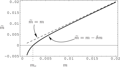
Figure 1: The physical mass vs. bare mass in units of the noncommutative scale $\lambda_{\rm nc}$ (or Planck length ${\lambda_{\mathbf{P}}}$). The graph is plotted with Mathematica 5.0 for $m\in[0.001,0.02]\cdot\lambda_{\rm nc}^{-1}$. The straight line corresponds to $\widetilde{m}=m-\delta m$ and the dashed line to $\widetilde{m}=m$.

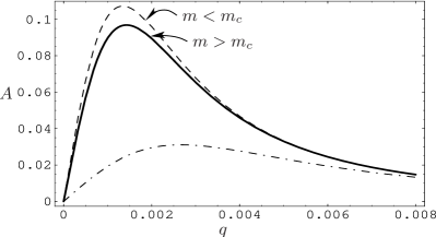
Figure 2: Radial deviation $A(q)=v(q)-\tilde{v}(q)$ of the group-velocity in units of the noncommutative scale $\lambda_{\rm nc}$ (or Planck length ${\lambda_{\mathbf{P}}}$). The graph is plotted with Mathematica 5.0 for $q\in[0,0.008]$. The straight line corresponds to $m=2.4\cdot 10^{-3}\cdot\lambda_{\rm nc}^{-1}$, the dashed line to $m=2.3\cdot 10^{-3}\cdot\lambda_{\rm nc}^{-1}$ and the dashed-dotted line to $m=4.0\cdot 10^{-3}\cdot\lambda_{\rm nc}^{-1}$.

The group-velocity can also be calculated:

$$\mathbf{v}({\mathbf{q}})=\nabla_{\mathbf{q}}E({\mathbf{q}})\ .$$

The energy correction up to second order is $E({\mathbf{q}})=\omega_{\mathbf{q}}-\delta E({\mathbf{q}})$. Obviously $\mathbf{v}({\mathbf{q}})$ is again covariant under rotation and translation, but not covariant under Lorentz transformation. Therefore we take again spherical coordinates $q:=|{\mathbf{q}}|,\theta,\varphi$ and use the fact that $|\mathbf{v}({\mathbf{q}})|=v(q)$:

$$v(q)=\frac{q}{\sqrt{q^{2}+m^{2}}}-\frac{\partial}{\partial q}\delta E(q)\ .$$ (13)

In doing so, $v(q)$ can be compared with the Lorentzian invariant group velocity corresponding to the renormalised mass:

$$\tilde{v}(q):=\frac{q}{\sqrt{q^{2}+(m-\delta m)^{2}}}\ .$$

The radial deviation $A(q)$ is then given by:

$$A(q)=v(q)-\tilde{v}(q)\ .$$

This deviation is plotted in FIG. 2 for three different masses in units of the noncommutative scale (Planck mass): straight line for $m=2.4\cdot 10^{-3}\cdot\lambda_{\rm nc}^{-1}$, dashed line for $m=2.3\cdot 10^{-3}\cdot\lambda_{\rm nc}^{-1}$ and dashed-dotted line for $m=4.0\cdot 10^{-3}\cdot\lambda_{\rm nc}^{-1}$; the momentum runs in the range $q\in[0,0.008]\times\lambda_{\rm nc}^{-1}$ in units of the noncommutativity parameter $\lambda_{\rm nc}$.

III Discussion

If we take a closer look at the connection between the physical mass and the bare mass in FIG. 1 we find that for particles with a physical mass of magnitude ranging from GeV to TeV and even for particles with $\widetilde{m}=0$, we have a finite bare mass $m\geq m_{\rm c}>0$ of order $>10^{-3}\cdot\lambda_{\rm nc}$. If we plug in the Planck length, the critical bare mass is about $m_{\rm c}\approx 2.8279\cdot 10^{16}$GeV and thus (accidentally) at the mass scale of the Grand Unified Theories (GUTs).

The dispersion relation in FIG. 2 can be interpreted in two ways. First we consider a general undetermined noncommutativity parameter $\lambda_{\rm nc}$. Then a maximal deviation of $A(q)\approx 0.03$ in the group velocity of a particle at momentum $q\approx 86$GeV and a physical mass of $\widetilde{m}\approx 80$GeV yields a bare mass $m\approx 128$GeV and a noncommutativity parameter $\lambda_{\rm nc}^{-1}\approx 32$TeV, while a maximal deviation of $A(q)\approx 0.095$ at momentum $q\approx 764$GeV of a particle with physical mass $\widetilde{m}\approx 90$GeV thus a bare mass $m\approx 1309.1$GeV leads to $\lambda_{\rm nc}^{-1}\approx 545,5$TeV. Therefore it should be possible to fix the energy bounds of the noncommutativity parameter $\lambda_{\rm nc}$ from experiment.

We can also consider the second case were $\lambda_{\rm nc}\equiv{\lambda_{\mathbf{P}}}$ and particles have physical masses of around 100GeV. For the dispersion relation we need to know the bare mass, which in this case is of course larger than $m_{\rm c}$ (of order $>10^{16}$GeV). Then the deviation $A(q)$ is a curve somewhere between the dashed and the straight line in FIG. 2 so that its local maximum is situated around $q\approx 0.0012\cdot{\lambda_{\mathbf{P}}}^{-1}$, which implies $q>10^{16}$GeV. If we now consider momenta of the order GeV to TeV we will not be able to detect any deviation in an experiment due to the vanishing of $A(q)$ in the limit $q\to 0$. We will see nothing of the noncommutative Minkowski space from this point of view. So the ansatz of the regularised, ultraviolet finite Hamilton operator on the noncommutative Minkowski space for regularising the UV- and the IR-regime does not contradict any experiment if we assume the Planck scale as the noncommutativity scale.

We may compare this with the Lorentzian invariant Yang-Feldman approach Bahns et al. (2005) and the recent works Doescher and Zahn (2006) on the noncommutative Minkowski space, where a deviation of the group velocity $v_{\bot}$ occurs (which in our approach is zero), which was shown to increase for decreasing masses. This is also true for our group velocity $v(q)$, but contrary to the Y-F-case, where the maximum is reached at zero momentum, our maximum is localised between $10^{-3}\cdotp\lambda_{\rm nc}$ and $\lambda_{\rm nc}$ and vanishes both for large and zero momentum (asymptotically free).

In Doescher and Zahn (2006) it is concluded that it is improbable to see detectable effects at LHC of the noncommutative Minkowski space in the Y-F-approach in the case $\lambda_{\rm nc}\equiv{\lambda_{\mathbf{P}}}$, if one chooses the typical parameter of the Higgs field. This is also the case in this approach due to the lower limit $m_{\rm c}$ of the bare mass and the very small energy correction at momenta of magnitude GeV to TeV.

*

Appendix A Energy correction in the vacuum state

In this appendix the energy correction in the vacuum state is calculated as an example. To keep the formulas short, the computations are restricted to a $\phi_{R}^{(3)}$-Theory; the general case can be performed in analogy. The notation is adapted from Bahns et al. (2003). Starting from equation (II):

$$\alpha_{2}[\Omega]=\frac{1}{3!^{2}} \int\frac{d{\mathbf{p}}_{1}d{\mathbf{p}}_{2}d{\mathbf{p}}_{3}}{\omega_{{\mathbf{p}}_{1}}+\omega_{{\mathbf{p}}_{2}}+\omega_{{\mathbf{p}}_{3}}}\Big{[}$$

$$\int d{\mathbf{x}}d{\mathbf{y}}\lambda({\mathbf{x}})\lambda({\mathbf{y}})\left\langle{\Omega}\right|\text{\bf:}\phi_{R}^{(3)}(0,{\mathbf{x}})\text{\bf:}\left|{p_{1}p_{2}p_{3}}\right\rangle$$

$$\quad\quad\left\langle{p_{1}p_{2}p_{3}}\right|\text{\bf:}\phi_{R}^{(3)}(0,{\mathbf{y}})\text{\bf:}\left|{\Omega}\right\rangle\Big{]}\ ,$$

we calculate first the following integral by standard methods:
$\int d{\mathbf{x}}\lambda({\mathbf{x}})\left\langle{\Omega}\right|\text{\bf:}\phi_{R}^{(3)}(0,{\mathbf{x}})\text{\bf:}\left|{p_{1}p_{2}p_{3}}\right\rangle=$

$$= \frac{c_{3}}{3^{4}}\frac{1}{\sqrt{3!}}\int d\underline{a}_{1}\ \lambda({\bm{\kappa}}(\underline{\mathbf{a}}_{1}))e^{-\frac{1}{2}|\underline{\mathbf{a}}_{1}-{\bm{\kappa}}(\underline{\mathbf{a}}_{1})|^{2}}\ e^{-\frac{1}{2}|\underline{a}^{0}_{1}|^{2}}$$

$$\quad\times\quad\delta(\kappa^{0}(\underline{a}_{1}^{0}))\left\langle{\Omega}\right|\text{\bf:}\phi(a_{11})\phi(a_{21})\phi(a_{31})\text{\bf:}a^{+}_{{\mathbf{p}}_{1}}a^{+}_{{\mathbf{p}}_{2}}a^{+}_{{\mathbf{p}}_{3}}\left|{\Omega}\right\rangle$$

$$= \frac{c_{3}}{3^{4}}\frac{1}{\sqrt{3!}}\frac{1}{(2\pi)^{9/2}}\tfrac{1}{\sqrt{8}}\sum_{\pi}\int d\underline{a}_{1}\ \lambda({\bm{\kappa}}(\underline{\mathbf{a}}_{1}))$$

$$\times\ e^{-\frac{1}{2}|\underline{\mathbf{a}}_{1}-\kappa(\underline{\mathbf{a}}_{1})|^{2}}e^{-\frac{1}{2}|\underline{a}^{0}_{1}|^{2}}\delta(\kappa^{0}(\underline{a}_{1}^{0}))\Big{\{}$$

$$\times\ \frac{e^{-ip_{\pi(1)}a_{11}}e^{-ip_{\pi(2)}a_{21}}e^{-ip_{\pi(3)}a_{31}}}{\sqrt{\omega_{{\mathbf{p}}_{1}}\omega_{{\mathbf{p}}_{2}}\omega_{{\mathbf{p}}_{3}}}}\Big{\}}\ \ .$$

The sum runs over all permutations $\pi$ and in analogy we obtain:
$\int d{\mathbf{y}}\lambda({\mathbf{y}})\left\langle{p_{1}p_{2}p_{3}}\right|\text{\bf:}\phi_{R}^{(3)}(0,{\mathbf{y}})\text{\bf:}\left|{\Omega}\right\rangle=$

$$= \frac{c_{3}}{3^{4}}\frac{1}{\sqrt{3!}}\int d\underline{a}_{2}\ \lambda({\bm{\kappa}}(\underline{\mathbf{a}}_{2}))e^{-\frac{1}{2}|\underline{\mathbf{a}}_{2}-{\bm{\kappa}}(\underline{\mathbf{a}}_{2})|^{2}}e^{-\frac{1}{2}|\underline{a}^{0}_{2}|^{2}}$$

$$\ \times\ \delta(\kappa^{0}(\underline{a}_{2}^{0}))\left\langle{\Omega}\right|a_{{\mathbf{p}}_{1}}a_{{\mathbf{p}}_{2}}a_{{\mathbf{p}}_{3}}\text{\bf:}\phi(a_{12})\phi(a_{22})\phi(a_{32})\text{\bf:}\left|{\Omega}\right\rangle$$

$$= \frac{c_{3}}{3^{4}}\frac{1}{\sqrt{3!}}\frac{1}{(2\pi)^{9/2}}\frac{1}{\sqrt{8}}\sum_{\sigma}\int d\underline{a}_{2}\ \lambda({\bm{\kappa}}(\underline{\mathbf{a}}_{2}))e^{-\frac{1}{2}|\underline{\mathbf{a}}_{2}-{\bm{\kappa}}(\underline{\mathbf{a}}_{2})|^{2}}$$

$$\times\ e^{-\frac{1}{2}|\underline{a}^{0}_{2}|^{2}}\delta(\kappa^{0}(\underline{a}_{2}^{0}))\frac{e^{ip_{\sigma(1)}a_{12}}e^{ip_{\sigma(2)}a_{22}}e^{ip_{\sigma(3)}a_{32}}}{\sqrt{\omega_{{\mathbf{p}}_{1}}\omega_{{\mathbf{p}}_{2}}\omega_{{\mathbf{p}}_{3}}}}\ .$$

The following transformations are similar to the one in Bahns et al. (2003) and render the Gaussian functions independent of one of the integration variables. First of all we redefine the momenta:

$$U^{\prime}_{1}\underline{k}_{1}:=-\left(\begin{matrix}I&0&0\\ 0&I&0\\ 0&0&I\\ \end{matrix}\right)\left(\begin{matrix}p_{\pi(1)}\\ p_{\pi(2)}\\ p_{\pi(3)}\\ \end{matrix}\right)\ ,$$

$$U^{\prime}_{2}\underline{k}_{2}:=\left(\begin{matrix}I&0&0\\ 0&I&0\\ 0&0&I\\ \end{matrix}\right)\left(\begin{matrix}p_{\sigma(1)}\\ p_{\sigma(2)}\\ p_{\sigma(3)}\\ \end{matrix}\right)\ .$$

These expressions substituted into the upper integrals leads to the following:

$$\int{d\underline{\mathbf{a}}_{1}d\underline{\mathbf{a}}_{2}}\ \lambda({\bm{\kappa}}(\underline{\mathbf{a}}_{1}))\lambda({\bm{\kappa}}(\underline{\mathbf{a}}_{2}))e^{-\frac{1}{2}|\underline{\mathbf{a}}_{1}-{\bm{\kappa}}(\underline{\mathbf{a}}_{1})|^{2}}e^{-\frac{1}{2}|\underline{\mathbf{a}}_{2}-{\bm{\kappa}}(\underline{\mathbf{a}}_{2})|^{2}}\$$

$$\times\quad\quad e^{i{\mathbf{U}}_{1}\underline{\mathbf{k}}_{1}\underline{\mathbf{a}}_{1}}e^{i{\mathbf{U}}_{2}\underline{\mathbf{k}}_{2}\underline{\mathbf{a}}_{2}}$$

$$\times\int d\underline{a}_{1}^{0}d\underline{a}_{2}^{0}\ e^{-\frac{1}{2}|\underline{a}_{1}^{0}|^{2}}e^{-\frac{1}{2}|\underline{a}_{2}^{0}|^{2}}\delta(\kappa^{0}(\underline{a}_{1}^{0}))\delta(\kappa^{0}(\underline{a}_{2}^{0}))$$

$$\times\quad\quad e^{iU_{1}\underline{k}_{1}^{0}\underline{a}_{1}^{0}}e^{iU_{2}\underline{k}_{2}^{0}\underline{a}_{2}^{0}}\ .$$

The techniques also used in (Bahns et al., 2003, appendix) yield Gaussian functions in $N(n-1)$ coordinates and an integral over $N$ coordinates $\beta_{M}=(\beta^{0}_{M},{\bm{\beta}}_{M}):=(b^{0}_{nM},{\mathbf{b}}_{nM})$:

$$(2\pi)^{6}\ e^{-\frac{1}{2}|({\mathbf{I}}-{\mathbf{P}}){\mathbf{U}}_{1}\underline{\mathbf{k}}_{1}|^{2}}e^{-\frac{1}{2}|({\mathbf{I}}-{\mathbf{P}}){\mathbf{U}}_{2}\underline{\mathbf{k}}_{2}|^{2}}$$

$$\times\int{d{\bm{\beta}}_{1}d{\bm{\beta}}_{2}}\ \lambda({\bm{\beta}}_{1}/\sqrt{3})\lambda({\bm{\beta}}_{2}/\sqrt{3})$$

$$\times\quad\quad e^{i({\mathbf{V}}_{\underline{e}_{3}}{\mathbf{R}}{\mathbf{U}}_{1}\underline{\mathbf{k}}_{1})\cdot{\bm{\beta}}_{1}}e^{i({\mathbf{V}}_{\underline{e}_{3}}{\mathbf{R}}{\mathbf{U}}_{2}\underline{\mathbf{k}}_{2})\cdot{\bm{\beta}}_{2}}$$

$$\times\ \int d\underline{b}_{1}^{0}d\underline{b}_{2}^{0}\ e^{-\frac{1}{2}(|\underline{b}_{1}^{0}|^{2})}e^{-\frac{1}{2}(|\underline{b}_{2}^{0}|^{2})}\delta\left(\tfrac{b_{31}^{0}}{\sqrt{3}}\right)\delta\left(\tfrac{b_{32}^{0}}{\sqrt{3}}\right)\$$

$$\times\quad\quad e^{i(RU_{1}\underline{k}_{1}^{0})\underline{b}_{1}^{0}}e^{i(RU_{2}\underline{k}_{2}^{0})\underline{b}_{2}^{0}}\ .$$

Performing the time-like integration in the variables $b_{11}^{0},\ b_{21}^{0},\ b_{12}^{0},b_{22}^{0}$ and setting $\beta_{i}=b_{3i}$ we get:

$$(2\pi)^{6}\ e^{-\frac{1}{2}|({\mathbf{I}}-{\mathbf{P}}){\mathbf{U}}_{1}\underline{\mathbf{k}}_{1}|^{2}}e^{-\frac{1}{2}|({\mathbf{I}}-{\mathbf{P}}){\mathbf{U}}_{2}\underline{\mathbf{k}}_{2}|^{2}}$$

$$\times\ (2\pi)^{2}\int{d{\bm{\beta}}_{1}d{\bm{\beta}}_{2}}\ \lambda({\bm{\beta}}_{1}/\sqrt{3})\lambda({\bm{\beta}}_{2}/\sqrt{3})e^{i({\mathbf{V}}_{\underline{e}_{3}}{\mathbf{R}}{\mathbf{U}}_{1}\underline{\mathbf{k}}_{1})\cdot{\bm{\beta}}_{1}}$$

$$\times\ e^{i({\mathbf{V}}_{\underline{e}_{3}}{\mathbf{R}}{\mathbf{U}}_{2}\underline{\mathbf{k}}_{2})\cdot{\bm{\beta}}_{2}}e^{-\frac{1}{2}|(I-P)U_{1}\underline{k}_{1}^{0}|^{2}}e^{-\frac{1}{2}|(I-P)U_{2}\underline{k}_{2}^{0}|^{2}}$$

$$\times\ \int d\beta_{1}^{0}d\beta_{2}^{0}\ e^{-\frac{1}{2}|\beta_{1}^{0}|^{2}}e^{-\frac{1}{2}|\beta_{2}^{0}|^{2}}\delta\left(\tfrac{\beta_{1}^{0}}{\sqrt{3}}\right)\delta\left(\tfrac{\beta_{2}^{0}}{\sqrt{3}}\right)$$

$$\times\ e^{i(V_{\underline{e}_{3}}RU_{1}\underline{k}_{1}^{0})\beta_{1}^{0}}e^{i(V_{\underline{e}_{3}}RU_{2}\underline{k}_{2}^{0})\beta_{2}^{0}}\ .$$

The last two lines give just the number of the Wickpower $n$ (i.e. 3). We can not set $\lambda({\bm{\beta}}_{i})\to 1$ in the second line since we would obtain the square of a delta function. So we use the relation $V_{\underline{e}_{n}}RU_{1}\underline{k}_{1}^{\mu}=\underline{{\xi}}\cdot(U_{1}\underline{k}^{\mu})=\tfrac{1}{\sqrt{n}}\sum_{i}^{n}u_{ii1}k_{i1}^{\mu}$ (see Bahns et al. (2003)) and obtain the following expression ($p^{0}=\omega_{\mathbf{p}}$):

$$\tilde{c}\sum_{\pi,\sigma} \int\frac{d{\mathbf{p}}_{1}d{\mathbf{p}}_{2}d{\mathbf{p}}_{3}\ }{(\omega_{{\mathbf{p}}_{1}}+\omega_{{\mathbf{p}}_{2}}+\omega_{{\mathbf{p}}_{3}}){\omega_{{\mathbf{p}}_{1}}\omega_{{\mathbf{p}}_{2}}\omega_{{\mathbf{p}}_{3}}}}$$

$$\times\ |\check{\lambda}(\tfrac{1}{{3}}({\mathbf{p}}_{1}+{\mathbf{p}}_{2}+{\mathbf{p}}_{3}))|^{2}$$

$$\times\ \prod_{j=1}^{3}e^{-\frac{1}{2}|p_{\pi(j)}-\frac{1}{3}\sum_{i=1}^{3}p_{\pi(i)}|^{2}}e^{-\frac{1}{2}|p_{\sigma(j)}-\frac{1}{3}\sum_{i=1}^{3}p_{\sigma(i)}|^{2}}\ .$$

The constant in front of the sum is $\tilde{c}:=\frac{c_{3}^{2}}{3!^{2}}\frac{1}{{3!}}\frac{1}{(2\pi)^{9}}\frac{3(2\pi)^{8}}{3^{8}8}$ and $c_{n}=n^{2}(2\pi)^{-2(n-1)}$. For each permutation the summands have the same value. Therefore we obtain the following integral, which is not defined for $\lambda({\mathbf{x}})\to 1$ since in Fourier space $|\check{\lambda}({\mathbf{p}})|^{2}\to|\delta({\mathbf{p}})|^{2}$ would tend to the square of a delta function:

$$\frac{1}{3^{4}}\frac{1}{(2\pi)^{9}}\frac{1}{16} \int\frac{d{\mathbf{p}}_{1}d{\mathbf{p}}_{2}d{\mathbf{p}}_{3}\ }{(\omega_{{\mathbf{p}}_{1}}+\omega_{{\mathbf{p}}_{2}}+\omega_{{\mathbf{p}}_{3}}){\omega_{{\mathbf{p}}_{1}}\omega_{{\mathbf{p}}_{2}}\omega_{{\mathbf{p}}_{3}}}}$$

$$\times\ |\check{\lambda}(\tfrac{1}{{3}}({\mathbf{p}}_{1}+{\mathbf{p}}_{2}+{\mathbf{p}}_{3}))|^{2}$$

$$\times\ \prod_{j=1}^{3}e^{-|p_{j}-\frac{1}{3}\sum_{i=1}^{3}p_{i}|^{2}}\ .$$

The problem of the occurrence of the square of a delta function is absent in the one particle term due to different momenta.

With this procedure one can in principle calculate the correction of the improper one particle state or also multiparticle states to higher orders and/or higher powers of the regularised Wick monomials.

References

• Snyder (1947) H. S. Snyder, Phys. Rev. 71, 38 (1947).
• Doplicher (2001) S. Doplicher (2001), eprint hep-th/0105251.
• Doplicher et al. (1995) S. Doplicher, K. Fredenhagen, and J. E. Roberts, Commun. Math. Phys. 172, 187 (1995), eprint hep-th/0303037.
• Bahns et al. (2002) D. Bahns, S. Doplicher, K. Fredenhagen, and G. Piacitelli, Phys. Lett. B533, 178 (2002), eprint hep-th/0201222.
• Bahns (2003) D. Bahns, Fortsch. Phys. 51, 658 (2003), eprint hep-th/0212266.
• Bahns et al. (2005) D. Bahns, S. Doplicher, K. Fredenhagen, and G. Piacitelli, Phys. Rev. D71, 025022 (2005), eprint hep-th/0408204.
• Bahns et al. (2003) D. Bahns, S. Doplicher, K. Fredenhagen, and G. Piacitelli, Commun. Math. Phys. 237, 221 (2003), eprint hep-th/0301100.
• Minwalla et al. (2000) S. Minwalla, M. Van Raamsdonk, and N. Seiberg, JHEP 02, 020 (2000), eprint hep-th/9912072.
• Rivasseau et al. (2006) V. Rivasseau, F. Vignes-Tourneret, and R. Wulkenhaar, Commun. Math. Phys. 262, 565 (2006), eprint hep-th/0501036.
• Grosse and Steinacker (2006) H. Grosse and H. Steinacker (2006), eprint hep-th/0607235.
• Bahns (2004) D. Bahns (2004), DESY-THESIS-2004-004.
• Denk et al. (2004) S. Denk, V. Putz, M. Schweda, and M. Wohlgenannt, Eur. Phys. J. C35, 283 (2004), eprint hep-th/0401237.
• Piacitelli (2004) G. Piacitelli (2004), eprint hep-th/0403055.
• Reed and Simon (1975) M. Reed and B. Simon, Methods of Modern Mathematical Physics, vol. I-IV (Academic Press Inc., 1975).
• Doescher and Zahn (2006) C. Doescher and J. Zahn (2006), eprint hep-th/0605062.