Realistic Yukawa Couplings through Instantons in Intersecting Brane Worlds

Abstract:

The Yukawa couplings of the simpler models of D-branes on toroidal orientifolds suffer from the so-called “rank one” problem – there is only a single non-zero mass and no mixing. We consider the one-loop contribution of E2-instantons to Yukawa couplings on intersecting D6-branes, and show that they can solve the rank one problem. In addition they have the potential to provide a geometric explanation for the hierarchies observed in the Yukawa coupling. In order to do this we provide the necessary quantities for instanton calculus in this class of background.

1 Introduction

Intersecting D-branes are an interesting possibility for string model building, allowing one to build models that come remarkably close to the MSSM in terms of particle content and gauge group. A particularly simple and calculable subset of these are models constructed from D6-branes in type IIA string theory, wrapping orientifolds of $\mathbb{R}_{4}\times\mathbb{T}_{2}\times\mathbb{T}_{2}\times\mathbb{T}_{2}$ (see e.g. [1]-[14] or [15] for a review). One of the interesting features of these models is that the localization of matter fields at D-brane intersections may have implications for a number of phenomenological questions, most notably the flavour structure of the Yukawa couplings [16]. Initially it was thought that these could be understood by having the matter fields in the coupling located at different intersections, with the resulting coupling being suppressed by the classical world-sheet instanton action (the minimal world-sheet area in other words). Since the resulting Yukawa couplings are of the form

$$Y\propto e^{-Area/2\pi\alpha^{\prime}}$$

the hope was that one would be able to find a geometric explanation of the mass and mixing hierarchies of the MSSM. Not only would this be simple and elegant, but it would also mean that measurements of the Yukawa couplings of the MSSM would yield direct information about the compactification geometry. Unfortunately in the simplest compactifications this hope was misplaced. The reason why is the so-called “rank one” problem; the simplest models have left-handed fields separated in one $\mathbb{T}_{2}$, and right-handed fields separated in a different $\mathbb{T}_{2}$, and the couplings had a rank one flavour structure,

$$Y^{0}_{ab}\sim A_{a}B_{b},$$

where $a,b$ label flavour and $A,B$ are two vectors whose elements are sensitive to the displacements of vertices in the compact dimensions. Only the third generation gets a mass and there is no mixing.

There have been numerous subsequent attempts to solve this problem as well as other related analyses of questions regarding flavour (e.g. refs.[17]-[25]), but many of these lost the original link with geometry. In parallel there developed techniques for calculating both tree level [26]-[31], and loop [32]-[34] amplitudes involving chiral (intersection) states on networks of intersecting D-branes.

The most recent development on the calculational side, whose consequences will be the subject of this paper, has been the incorporation of the effect of instantons in ref.[35] (for related work see also [36]-[39]). This work laid out in detail how the contributions of so-called E2-instantons (i.e. branes with 3 Neumann boundary conditions in the compact dimensions and Dirichlet boundary conditions everywhere else) to the superpotential could be calculated. It also pointed out a number of expected phenomenological consequences of these objects. Thus far attention has mostly been paid to the fact that instantons do not necessarily respect the global symmetries of the effective theory and so are able to generate terms that may otherwise be disallowed. In particular they can be charged under the parent anomalous U(1)’s due to the Green-Schwarz anomaly cancellation mechanism. (Alternatively, these charges can be associated with states at the intersection of the E2 and D6 branes.) For example this can induce Majorana mass terms for neutrinos which are of the form

$$e^{-\frac{8\pi^{2}}{g_{E2}^{2}}}M_{s}\nu_{R}\nu_{R}\,,$$

and which would otherwise be forbidden. In this equation $g_{E2}$ is an effective coupling strength which depends on the world-volume of the E2 instanton. These need not be equal to the gauge couplings of the MSSM and the Majorana mass-terms can be of the right order to generate the observed neutrino masses [35],[37]. Similarly interesting contributions occur for the $\mu$-term of the MSSM, yielding a possible solution to the $\mu$-problem.

In this paper we reassess Yukawa couplings in the light of instanton contributions. In particular we claim that one-loop diagrams with E2 branes can solve the rank-one problem and lead to a Yukawa structure which is hierarchical. All the Yukawa couplings have by assumption the same charges under all symmetries, so the extra terms are induced by E2 instantons which do not intersect the D6-branes. The tree and one-loop contributions to Yukawa couplings are shown in figure 1; the tree level diagram consists of the usual disc diagram with three vertices, the one loop diagram is an annulus with the inside boundary being an E2 brane and three vertices on the D6-brane boundary. By explicit computation of these one-loop instanton contributions we show that the corrected Yukawas are of the form

$$Y_{ab}=Y^{0}_{ab}+Y^{np}_{ab},$$

where the nonperturbative contribution has rank 3. Moreover as for the neutrino Majorana masses, these contributions are exponentially suppressed by the instanton volume. Hence the 1st and 2nd generation masses are hierarchically smaller than the first.

In addition there is the possibility of making an interesting connection between the Yukawa hierarchies and the Majorana neutrino masses. The suppression of the latter with respect to the string scale should be similar to the suppression of 2nd generation masses with respect to third generation ones. In general one sees that a direct connection between compactification geometry and Yukawa couplings would be manifest. The rest of this paper is devoted to proving this result. In the next section we outline the techniques of instanton calculus and compute the necessary general results: these include the multiplying factors of disconnected tree-level and one-loop diagrams with no vertex operators, which must appear in every such process. The section that follows provides the annulus correlator, and in particular shows that the leading contribution yields instanton contributions to the Yukawa couplings of the advertised form.

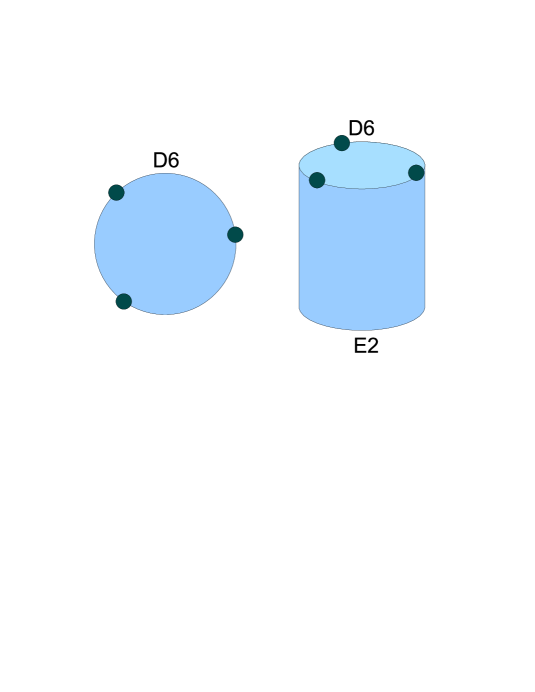
Figure 1: Contributions to 3 point functions: tree level and one-loop instanton.

2 Instanton Calculus

The general framework for calculating E2 instanton corrections to the superpotential in string backgrounds was proposed in [35]. This section elucidates the technical details of the calculus of E2 instanton corrections applied to toroidal orientifold intersecting brane worlds.

2.1 Tree Level Contributions

The non-perturbative $O(e^{-8\pi^{2}/g_{E2}^{2}})$ factor appearing in instanton contributions to the superpotential is given by the product of all possible disk diagrams whose boundary lies along the instanton and with either no vertex operators or an RR-tadpole operator. We shall label this contribution $e^{-S^{0}_{E2}}$. It is given by

$$S^{0}_{E2}=\frac{2\pi}{g_{s}\sqrt{(\alpha^{\prime})^{3}}}{L_{E2}}$$ (2.1)

where $L_{E2}=\prod_{\kappa=1}^{3}L^{\kappa}_{E2}$ is the volume of the instanton. The above can be given more conveniently in terms of the gauge coupling on a reference brane $a$ as

$$S^{0}_{E2}=8\pi^{2}\frac{L_{E2}}{L_{a}}g_{a}^{-2}$$ (2.2)

2.2 Pfaffians and Determinants

To perform any calculation in an E2 instanton background requires the knowledge of the reduced Pfaffian and Determinant factor given by the exponential of the total partition function of states intersecting the instanton with the zero modes removed. In toroidal backgrounds, there are two classes of contributions to this: the first arises when the instanton is parallel to a $D6$-brane in one torus, and the second appears when there is no parallel direction.

2.2.1 One Parallel Direction

In this case, there is no zero mode associated provided that the branes do not intersect, i.e. brane $a$ is separated from the E2 brane by some distance $y_{a,E2}$ in a torus $i$. In this case the partition function is given by

$$Z(E2,D6_{a}) = N_{a}I_{E2,a}^{j}I_{E2,a}^{k}\int\frac{\mathrm{d}t}{t}\sum_{\nu}\sum_{r^{i},s^{i}}\delta_{\nu}\frac{\theta_{\nu}^{2}(\frac{it}{2})}{\theta_{1}^{2}(\frac{it}{2})}\frac{\theta_{\nu}(\phi_{E2,a}it)\theta_{\nu}(-\phi_{E2,a}it)}{\theta_{1}(\phi_{E2,a}it)\theta_{1}(-\phi_{E2,a}it)}$$ (2.3)

$$\,\,\,\qquad\qquad\qquad\times\exp\bigg{[}\frac{-8\pi^{3}\alpha^{\prime}t}{(L_{E2}^{i})^{2}}|r^{i}+\frac{iT_{2}^{i}s^{i}}{\alpha^{\prime}}+\frac{iy_{a,E2}L_{E2}^{i}}{4\pi^{2}\alpha^{\prime}}|^{2}\bigg{]}$$

After performing the sum over spin structures we obtain an expression that would also be found in gauge threshold correction calculations

$$Z(E2,D6_{a})=N_{a}I_{E2,a}^{j}I_{E2,a}^{k}\int\frac{\mathrm{d}t}{t}\sum_{r^{i},s^{i}}\exp\bigg{[}\frac{-8\pi^{3}\alpha^{\prime}t}{(L_{E2}^{i})^{2}}|r^{i}+\frac{iT_{2}^{i}s^{i}}{\alpha^{\prime}}+\frac{iy_{a,E2}L_{E2}^{i}}{4\pi^{2}\alpha^{\prime}}|^{2}\bigg{]}.$$ (2.4)

This expression can be integrated. When all $y_{a,E2}\rightarrow 0$ (where there are fermionic zero modes that must be regulated) it gives [40]

$$Z(E2,D6_{a})_{y=0}=-N_{a}I_{E2,a}^{j}I_{E2,a}^{k}\left[\ln\frac{(L_{E2}^{i})^{2}}{\alpha^{\prime}}+\ln|\eta(\frac{T^{i}}{\alpha^{\prime}})|^{4}+\kappa\right],$$ (2.5)

where $\kappa=\gamma_{E}-\log 4\pi$ is a moduli-independent constant. For non-zero $y_{a,E2}$, the brane separation serves as an IR regulator to give

$$Z(E2,D6_{a})=-N_{a}I_{E2,a}^{j}I_{E2,a}^{k}\bigg{[}\log\left|\frac{\theta_{1}(\frac{iy_{a,E2}L_{E2}^{i}}{2\pi^{2}\alpha^{\prime}},\frac{iT_{2}^{i}}{\alpha^{\prime}})}{\eta(\frac{iT_{2}^{i}}{\alpha^{\prime}})}\right|^{2}-\frac{y_{a,E2}^{2}}{2\pi^{3}\alpha^{\prime}}\frac{(L_{E2}^{i})^{2}}{T_{2}^{i}}\bigg{]}\,.$$ (2.6)

This is derived in appendix A and agrees with [41]

It is noteworthy that the IR regularisation by separation of the $E2$ brane from brane $a$ does not commute with that used for $y_{a,E2}=0$. This reflects the qualitative difference between E2 branes which wrap cycles where $b_{1}(\Pi_{E2})=0$ and those where the betti number is non-zero; in the latter case (i.e. when the instanton does not pass through a fixed point) it acquires additional uncharged fermionic zero modes which must be integrated over, but when the separation between D6 and E2 branes reduces to zero there arise additional charged fermionic zero modes. We only consider configurations with no additional zero modes in this paper, and thus we require the E2 branes to pass through fixed points and D6 branes to be separated from these by some small distances. This is a common feature of many models, although it is incompatible with the models of, for example, [13, 14]. However, since the extra uncharged modes carry no coupling, it is actually possible for E2 instantons with six additional uncharged zero modes to contribute to the superpotential term considered in this paper generated at one loop, and thus we expect our conclusions to extend to those models as well. As explored recently in [42, 43, 44], this can occur when there are non-zero bulk fluxes threading the E2 brane worldvolume (which are naturally present in models to stabilise moduli), but in that case the exact calculation of the superpotential contribution is beyond the scope of this paper.

2.2.2 No Parallel Directions

Here we have the raw expression

$$Z(E2,D6_{a})=N_{a}I_{E2,a}\int\frac{\mathrm{d}t}{t}\sum_{\nu}\delta_{\nu}\frac{\theta_{\nu}^{2}(\frac{it}{2})}{\theta_{1}^{2}(\frac{it}{2})}\frac{\eta^{3}(it)}{\theta_{\nu}(0)}\prod_{\kappa=1}^{3}\frac{\theta_{\nu}(\phi^{\kappa}_{E2,a}it)}{\theta_{1}(\phi^{\kappa}_{E2,a}it)}.$$ (2.7)

However, this amplitude is not defined in the $\nu=1$ sector, and additionally contains fermionic zero modes which must be regularised. The first issue is straightforward to resolve: provided that the model satisfies RR-charge cancellation, the $\nu=1$ sector does not contribute. To address the second issue we must decide how to remove the zero mode from the trace over states: this is trivial once we express the amplitude in the open string channel. Since the integral over the modular parameter and the exponentiation of the partition function translates the sum over states into a product, it is clear that we must simply expand the partition function as a series in $e^{-\pi t}$ and remove the $O(1)$ term in the $\nu=1,2$ sectors. The piece subtracted turns out to be cancelled over all the contributions by the RR cancellation condition, and so we can ignore it.

We must now perform the sum over spin structures. To this end, we use the identity

$$\left(\frac{\theta_{\nu}(z)\theta_{1}^{\prime}(0)}{\theta_{1}(z)\theta_{\nu}(0)}\right)^{2}=\frac{\theta_{\nu}^{\prime\prime}(0)}{\theta_{\nu}(0)}-\partial^{2}\log\theta_{1}(z)$$ (2.8)

to write the partition function as

$$Z(E2,D6_{a})=N_{a}I_{E2,a}\int\frac{\mathrm{d}t}{t}\sum_{\nu\neq 1}\delta_{\nu}\bigg{[}\theta_{\nu}^{\prime\prime}(0)-\theta_{\nu}(0)\partial^{2}\log\theta_{1}(\frac{it}{2})\bigg{]}\frac{1}{2\pi\theta_{1}^{\prime}(0)}\prod_{\kappa=1}^{3}\frac{\theta_{\nu}(\phi^{\kappa}_{E2,a}it)}{\theta_{1}(\phi^{\kappa}_{E2,a}it)}.$$ (2.9)

It is straightforward to show that, if we were to include the $\nu=1$ term to the above, it would not contribute, and hence we can perform the spin structure sum using the usual Riemann theta identities. The term proportional to $\theta_{\nu}(0)$ vanishes, and we have remaining an expression identical to that found in gauge threshold corrections. The calculation is then that of [40, 45], including the cancellation of divergences arising in the NS sector. The result is then

$$\frac{\mathrm{Pfaff}^{\prime}(D_{F})}{\sqrt{\det^{\prime}(D_{B})}}=\prod_{k}\left(\frac{\Gamma(1-2\phi_{E2,k}^{1})\Gamma(1-2\phi_{E2,k}^{2})\Gamma(1+2\phi_{E2,k}^{1}+2\phi_{E2,k}^{2})}{\Gamma(1+2\phi_{E2,k}^{1})\Gamma(1+2\phi_{E2,k}^{2})\Gamma(1-2\phi_{E2,k}^{1}-2\phi_{E2,k}^{2})}\right)^{-4I_{E2,O6_{k}}}\\ \prod_{a=\{a,a^{\prime}\}}\left(\frac{\Gamma(1-\phi_{E2,a}^{1})\Gamma(1-\phi_{E2,a}^{2})\Gamma(1+\phi_{E2,a}^{1}+\phi_{E2,a}^{2})}{\Gamma(1+\phi_{E2,a}^{1})\Gamma(1+\phi_{E2,a}^{2})\Gamma(1-\phi_{E2,a}^{1}-\phi_{E2,a}^{2})}\right)^{N_{a}I_{E2,a}}$$ (2.10)

This result, in contrast to that of the previous subsection, is not a holomorphic function of the moduli fields, and hence cannot contribute to the superpotential. This issue has recently been explored in [43], where they determined that the above generates the supergravity factor $e^{\frac{K}{2}}$ ($K$ being the Kähler potential) and Kähler potential normalisation for the charged zero modes, so indeed no contribution to the superpotential.

2.3 Vertex Operators and Zero Modes

Massless strings with at least one end on the E2 brane are the zero modes of the instanton. The most important of these (in that they are always present) are the fermionic modes with both ends on the E2 brane; these are the modes associated with the two broken supersymmetries in the spacetime dimensions. The vertex operator for toroidal models is thus

$$V^{-1/2}_{\theta}=\theta_{i}\tilde{S}^{i}\ e^{-\frac{\phi}{2}}\ \theta^{I}_{\alpha}\Theta^{\alpha}$$ (2.11)

where the internal spin field is $\Theta^{\alpha}=\prod_{\kappa=1}^{3}e^{\pm\frac{i}{2}H^{\kappa}}$; it is the spectral flow operator for the internal dimensions, or alternatively the internal part of the supercharge. This generically has four components after the GSO projection, and thus we have the eight modes of (broken) $N=4$, but only the two modes that preserve the same $N=1$ supersymetry as the branes and orientifolds in the model will contribute. In practice this involves choosing the correct $H$-charges to transform a fermion into a boson in the internal dimensions, and without loss of generality we shall take this to be $\prod_{\kappa=1}^{3}e^{-\frac{i}{2}H^{\kappa}}$. In addition, we may be concerned about antichiral bosonic zero modes that would spoil the generation of a superpotential. However, as discussed in [46, 47, 44], provided that the E2 brane is invariant under the orientifold projection, these will be removed from the spectrum.

Massless fermions at an intersection between the E2 brane and a D6 brane of the model are internal zero modes of the instanton. They will not be relevant for the following analysis, but are in general vitally important for calculations; we list their vertex operators here for completeness:

$$V_{\lambda_{a}} = \lambda_{a,I}^{i}e^{-\frac{\phi}{2}}\Delta\prod_{\kappa=1}^{3}e^{i(\phi_{aE2}^{\kappa}-1/2)H^{\kappa}}\sigma_{\phi_{aE2}^{\kappa}}$$

$$V_{\bar{\lambda_{b}}} = \bar{\lambda}_{b,I^{\prime}}^{i}e^{-\frac{\phi}{2}}\bar{\Delta}\prod_{\kappa=1}^{3}e^{i(\phi_{E2b}^{\kappa}-1/2)H^{\kappa}}\sigma_{\phi_{E2b}^{\kappa}}$$ (2.12)

where $I$ is the intersection number running from $1,...,[\Pi_{E2}\cap\Pi_{a}]^{+}$, and $I^{\prime}$ runs from $1,...,[\Pi_{E2}\cap\Pi_{b}]^{-}$ (note that $\phi_{E2b}-1/2=-(\phi_{bE2}-1/2)$); $i=1,..,N_{a}(N_{b})$ is the Chan-Paton index. $\Delta$ and $\bar{\Delta}$ are the boundary-changing operators in the four non-compact dimensions which interpolate between Dirichlet and Neumann boundary conditions; their OPE is

$$\Delta(z)\bar{\Delta}(w)\sim(z-w)^{-1/2}\,.$$ (2.13)

3 Yukawa Coupling Corrections

A straightforward analysis of the possible diagrams in the instanton calculus shows that in the presence of fermionic zero modes an $E2$-instanton cannot contribute to a Yukawa term in the superpotential for the quarks. However, if there exists one or more sLag cycles for which there are no intersections with any branes in the model, then a contribution to this term is possible through a one-loop annulus diagram. Typically this involves the separation of the $E2$-instanton from each D6 brane in one subtorus only, so that were the $E2$ brane replaced by a D6 brane wrapping the same three-cycle and the separations reduced to zero, this brane would preserve different $N=2$ supersymmetries with each of the branes in the model. This possibility arises generically but not in every case in model-building, so implies a new moderate constraint, in order to benefit from the consequences of these instantons.

To summarise the above and the conclusions of the previous section, in order to generate a correction to allowed superpotential couplings, then, we require

• $b_{1}(\Pi_{E2})=0$

• $[\Pi_{E2}\cap\Pi_{a}]=0\qquad\forall a$

• E2 brane invariant under orientifold projection, or suitable fluxes lifting bosonic zero modes

In the following we shall determine a contribution to the superpotential for an orientifold of $\mathbb{R}_{4}\times\mathbb{T}_{2}\times\mathbb{T}_{2}\times\mathbb{T}_{2}$, but expect our conclusions more generally to any model satisfying the above conditions, the further exploration of which we postpone to future work. In particular, we shall consider fractional E2 branes (under a suitable orbifold projection) to satisfy $b_{1}(\Pi_{E2})=0$ (for example in models with discrete torsion such as [13, 14, 48]) but bulk D6 branes. The annulus will only couple to the bulk component of the E2 brane, and hence the calculation is insensitive to the details of the orbifold projection.

A Yukawa superpotential term generated by E2 instantons involves three superfields on an annulus diagram, and thus two fermions and one boson together with two fermionic supersymmetry zero modes. We can then write (with vertex operators in the field theory basis, normalised by $V_{\phi_{ab}}\rightarrow\sqrt{K_{\phi_{ab}\bar{\phi}_{ab}}}V_{\phi_{ab}}$ from the string basis)[43]:

$$e^{\frac{K}{2}}W_{np}=\int\mathrm{d}^{4}x\mathrm{d}^{2}\theta\langle V^{0}_{\phi_{ab}}V^{1/2}_{\psi_{bc}}V^{1/2}_{\psi_{ca}}V^{-1/2}_{\theta}V^{-1/2}_{\theta}\rangle_{a,E2}\frac{\mathrm{Pfaff}^{\prime}(D_{F})}{\sqrt{\det^{\prime}(D_{B})}}e^{-S_{E2}^{0}}.$$ (3.1)

Since there are now three picture-changing operators in the above amplitude, to obtain a non-zero result we must apply each operator to a different subtorus direction; this is since each internal fermionic correlator must have zero net charge, and thus the charges introduced by the supersymmetry zero modes must be cancelled by those of the PCOs. The amplitude will then have no momentum prefactors, and thus will not factorise onto a scalar propagator; this is explicitly shown in appendix C.

Having determined the Pfaffian and Tree-level factors in section 2, we must now determine the annulus correlator. The total amplitude can be written as

$$\langle V^{0}_{\phi_{ab}}V^{1/2}_{\psi_{bc}}V^{1/2}_{\psi_{ca}}V^{-1/2}_{\theta}V^{-1/2}_{\theta}\rangle_{a,E2}=\phi_{(ab)}\psi_{(bc)\alpha}C^{\alpha\beta}\psi_{(ca)\beta}\ \theta_{1}\theta_{2}\\ \times\int\mathrm{d}t\ it\prod_{i=2}^{3}\int_{0}^{it}\mathrm{d}z_{i}\prod_{j=1}^{2}\int_{1/2}^{1/2+it}\mathrm{d}w_{j}\langle e^{\frac{\phi}{2}(z_{2})}e^{\frac{\phi}{2}(z_{3})}e^{-\frac{\phi}{2}(w_{1})}e^{-\frac{\phi}{2}(w_{2})}\rangle\lim_{x_{1}\rightarrow z_{1}}\lim_{x_{2}\rightarrow z_{2}}\lim_{x_{3}\rightarrow z_{3}}\\ \times(x_{1}-z_{1})(x_{2}-z_{2})^{1/2}(x_{3}-z_{3})^{1/2}\langle\tilde{S}^{1}(z_{2})\tilde{S}^{1}(z_{3})\tilde{S}^{2}(w_{1})\tilde{S}^{2}(w_{2})\rangle\langle\prod_{i=1}^{3}e^{ik_{i}\cdot X(z_{i})}\rangle\\ \sum_{\{y_{1},y_{2},y_{3}\}=P(x_{1},x_{2},x_{3})}\prod_{\kappa=1}^{3}\sqrt{\frac{2}{\alpha^{\prime}}}\langle\partial\bar{X}^{\kappa}(y_{\kappa})\sigma_{\phi^{\kappa}_{ab}}(z_{1})\sigma_{\phi^{\kappa}_{bc}}(z_{2})\sigma_{\phi^{\kappa}_{ca}}(z_{3})\rangle\\ \times\langle e^{iH^{\kappa}(y_{\kappa})}e^{i(\phi_{(ab)}^{\kappa}-1)H^{\kappa}(z_{1})}e^{i(\phi_{(bc)}^{\kappa}-1/2)H^{\kappa}(z_{2})}e^{i(\phi_{(ca)}^{\kappa}-1/2)H^{\kappa}(z_{3})}e^{-\frac{i}{2}H^{\kappa}(w_{1})}e^{-\frac{i}{2}H^{\kappa}(w_{2})}\rangle$$ (3.2)

where $z_{1}$ has been fixed to $0$, and the angles $\phi^{\kappa}_{ab}$, $\phi^{\kappa}_{bc}$ and $\phi^{\kappa}_{ca}$ are external (hence $\phi^{\kappa}_{ab}+\phi^{\kappa}_{bc}+\phi^{\kappa}_{bc}=2$ and $\sum_{\kappa=1}^{3}\phi^{\kappa}=2$). $C^{\alpha\beta}=i(\Gamma^{1}\Gamma^{2})^{\alpha\beta}$ is the charge conjugation operator. The above amplitude can be evaluated using the techniques outlined in [32, 34]. The perhaps unexpected form of the spin-field correlator is explained in appendix B. The most non-trivial part of the above is that involving the boundary-changing operators, which are dominated by worldsheet-instanton effects. We split $\partial X=\partial X_{qu}+\partial X_{cl}$, for which $\partial X_{qu}$ has boundary conditions such that all vertices have no displacements, whereas $\partial X_{cl}$ absorbs the displacements between the vertices. We have

$$\langle\partial\bar{X}_{qu}\prod_{i=1}^{N}\sigma_{\phi_{i}}\rangle=0$$ (3.3)

and thus the amplitude is dominated by worldsheet instanton effects. To show the above, we consider

$$\frac{\langle\partial\bar{X}(w)\prod_{i=1}^{N}\sigma_{\phi_{i}}(z_{i})\rangle}{\langle\prod_{i=1}^{N}\sigma_{\phi_{i}}(z_{i})\rangle} \sim (w-z_{i})^{-\phi_{i}}\qquad w\rightarrow z_{i}$$

$$\frac{\langle\bar{\partial}\bar{X}(\bar{w})\prod_{i=1}^{N}\sigma_{\phi_{i}}(z_{i})\rangle}{\langle\prod_{i=1}^{N}\sigma_{\phi_{i}}(z_{i})\rangle} \sim (\bar{w}-\bar{z}_{i})^{\phi_{i}-1}\qquad\bar{w}\rightarrow\bar{z}_{i}$$ (3.4)

and construct a set of differentials satisfying the above local monodromies and periodicity of the worldsheet; these are the differentials given in [49, 32, 34]. We then apply the global monodromy

$$\int_{\gamma_{a}}\mathrm{d}w\partial\bar{X}+\mathrm{d}\bar{w}\bar{\partial}\bar{X}=\bar{v}_{a}$$ (3.5)

where $\gamma_{a}$ are a set of $N$ paths on the worldsheet and $v_{a}$ are the displacements between the vertices in the target space. There are $N$ independent differentials that comprise $\partial\bar{X}$ and $\bar{\partial}\bar{X}$, and so the global monodromies determine the coefficients by linear algebra. Since the paths are independent, the equations are non-degenerate and for $v_{a}=0$ we must set all of the coefficients to zero, establishing the claim above. Defining the $N\times N$ matrix $W$ ($i^{\prime}$ runs through the set $\{z_{1},z_{2},...,z_{N-2}\}$ and $i^{\prime\prime}$ denotes the complementary set $\{z_{N-1},z_{N}\}$):

$$W^{i^{\prime}}_{a} = \int_{\gamma_{a}}\mathrm{d}z\omega^{i^{\prime}}(z)$$

$$W^{i^{\prime\prime}}_{a} = \int_{\gamma_{a}}\mathrm{d}\bar{z}\bar{\omega}^{i^{\prime\prime}}(\bar{z})$$ (3.6)

in terms of the $N$ cut differentials $\{\omega^{i^{\prime}},\omega^{i^{\prime\prime}}\}$, we can then write (after applying the doubling trick to relate $\partial X$ to $\bar{\partial}\bar{X}$)

$$\langle\partial\bar{X}(x)\prod_{i=1}^{N}\sigma_{\phi_{i}}(z_{i})\rangle = -\bar{v}_{a}(\bar{W}^{-1})^{a}_{i^{\prime\prime}}\omega^{i^{\prime\prime}}(x)\langle\prod_{i=1}^{N}\sigma_{\phi_{i}}(z_{i})\rangle$$

$$\langle\bar{\partial}\bar{X}(\bar{x})\prod_{i=1}^{N}\sigma_{\phi_{i}}(z_{i})\rangle = -\bar{v}_{a}(\bar{W}^{-1})^{a}_{i^{\prime}}\bar{\omega}^{i^{\prime}}(-\bar{x})\langle\prod_{i=1}^{N}\sigma_{\phi_{i}}(z_{i})\rangle.$$ (3.7)

The correlator is thus directly proportional to the displacements. Specialising now to the specific three-point function and using the prescription of [34] we have cycles $\{\gamma_{a}\}=\{A,B,C_{2}\}$ where $A$ and $B$ are the canonical cycles of the torus, and $C_{2}$ is the path passing between two vertices on the worldsheet. For this diagram, in each subtorus there is one brane parallel to the $E2$ brane, and this represents a periodic cycle on the worldsheet. The prescription for the amplitude requires that we permute the vertices cyclically so that the periodic cycle passes along the real axis; writing $\{a^{\kappa},b^{\kappa},c^{\kappa}\}$ for the cyclic permutation of branes $\{a,b,c\}$ such that brane $a^{\kappa}$ is parallel to the E2 brane in torus $\kappa$, we have

$$v_{A} = \frac{1}{\sqrt{2}}n_{A}L_{a^{\kappa}}$$

$$v_{B} = i\sqrt{2}(n_{B}\frac{4\pi^{2}T_{2}^{\kappa}}{L_{a^{\kappa}}^{\kappa}}+y^{\kappa})$$

$$v_{C_{2}} = \frac{1}{\sqrt{2}}e^{i\phi_{a^{\kappa}c^{\kappa}}^{\kappa}}(n_{C}L_{c^{\kappa}}^{\kappa}+\Delta^{\kappa})$$ (3.8)

where $\Delta^{\kappa}$ is the shortest distance between the target-space intersections $b^{\kappa}c^{\kappa}$ and $c^{\kappa}a^{\kappa}$ along the brane $c^{\kappa}$, and $y^{\kappa}$ is the distance between $a^{\kappa}$ and the E2-brane. The phase $e^{i\phi_{a^{\kappa}c^{\kappa}}^{\kappa}}$ in the last line appears due to the orientation of brane $a^{\kappa}$ relative to $c^{\kappa}$.

The exponential of the worldsheet instanton action depends upon the same displacements, and the amplitude can then be schematically written as

$$\langle V^{0}_{\phi_{ab}}V^{1/2}_{\psi_{bc}}V^{1/2}_{\psi_{ca}}V^{-1/2}_{\theta}V^{-1/2}_{\theta}\rangle_{a,E2}=\phi_{(ab)}\psi_{(bc)\alpha}C^{\alpha\beta}\psi_{(ca)\beta}\big{(}\theta_{1}\theta_{2}-\theta_{2}\theta_{1}\big{)}\\ \int\mathrm{d}t\int\mathrm{d}z_{2}\mathrm{d}z_{3}\ \sum_{i=1}^{6}\prod_{\kappa=1}^{3}\bigg{(}\sum_{n^{\kappa}_{A},n^{\kappa}_{B},n^{\kappa}_{C}}\frac{(f_{i}^{\kappa})^{a}\bar{v}_{a}^{\kappa}}{\sqrt{\alpha^{\prime}}}e^{-\frac{S^{\kappa}}{2\pi\alpha^{\prime}}}\bigg{)}.$$ (3.9)

Note that the action which appears here is the one-loop action as derived from the monodromy conditions, and depends on the integration variables. The crucial part is that the functions $f_{i}$ arise from the different permutations of applications of the picture-changing operators. Each choice of $f_{i}$ corresponds to a different contribution that is separately factorisable across the tori (and different from the perturbative Yukawa term owing to the $\bar{v}_{a}^{\kappa}$ factors). Factorisability is in general lost upon performing the integral since there are no poles. However, since the functions are different, even if the integrals were dominated by a particular region of the moduli space, we would have Yukawa matrix corrections of the form

$$Y_{ab}\supset\sum_{i=1}^{6}A^{i}_{a}B^{i}_{b}\,.$$ (3.10)

This is a sum of six independent rank one matrices, giving a rank three Yukawa matrix as advertised in the introduction. Note that the correction terms are suppressed relative to the perturbative superpotential by approximately the factor $e^{-S_{E2}^{0}}$; this provides not only rank 3 couplings but an explanation for the hierarchy in masses between the top quark and the others. At the level of this analysis there is no obvious explanation for the hierarchies between the 1st and 2nd generation; this could yet arise from the non-factorisation of the worldsheet instanton contribution. We leave this issue for future work.

Appendix A Partition Function for Massive N=2 Sectors

In this appendix we evaluate the integral

$$Z(E2,D6_{a})=N_{a}I_{E2,a}^{j}I_{E2,a}^{k}\int\frac{\mathrm{d}t}{t}\sum_{r^{i},s^{i}}\exp\bigg{[}\frac{-8\pi^{3}\alpha^{\prime}t}{(L_{E2}^{i})^{2}}|r^{i}+\frac{iT_{2}^{i}s^{i}}{\alpha^{\prime}}+\frac{iy_{a,E2}L_{E2}^{i}}{4\pi^{2}\alpha^{\prime}}|^{2}\bigg{]}.$$ (A.1)

First we must Poisson-resum the expression on $r$ and $s$ to obtain

$$Z(E2,D6_{a}) = N_{a}I_{E2,a}^{j}I_{E2,a}^{k}\frac{(L_{E2}^{i})^{2}}{T_{2}^{i}}\frac{1}{8\pi^{2}}$$

$$\times\int_{0}^{\infty}\mathrm{d}l\sum_{m,n}\exp\bigg{[}-\frac{l(L_{E2}^{i})^{2}}{8\pi}\bigg{(}\frac{1}{\alpha^{\prime}}m^{2}+\frac{\alpha^{\prime}}{(T_{2}^{i})^{2}}n^{2}\bigg{)}-2in\frac{y_{a,E2}L_{E2}^{i}}{2\pi T_{2}^{i}}\bigg{]}\,.$$

We then note the divergence for the piece $m,n=0$ as $l\rightarrow\infty$ (and note that the separation between the branes will regulate any $l\rightarrow 0$ infra-red divergence). This arises in the NS sector and is cancelled for consistent models according to the condition [40]

$$\sum_{a=\{a,a^{\prime}\}}\frac{(L_{E2}^{i})^{2}}{T_{2}^{i}}N_{a}I_{E2,a}^{j}I_{E2,a}^{k}-4\sum_{\hat{k}}\frac{(L_{E2}^{i})^{2}}{T_{2}^{i}}I_{E2,O6_{\hat{k}}}^{j}I_{E2,O6_{\hat{k}}}^{k}=0.$$ (A.3)

This is sufficient if there are no intersections between the $E2$-brane and the $D6$-branes of the model; if there are branes for which there are no parallel dimensions then the cancellation condition will include those.

We now rescale the variables and perform the integral:

$$Z(E2,D6_{a})=N_{a}I_{E2,a}^{j}I_{E2,a}^{k}\frac{1}{\pi}\sum_{m,n\neq 0}\frac{\alpha^{\prime}}{T_{2}^{i}}\frac{\exp\bigg{[}-2\pi in\frac{y_{a,E2}L_{E2}^{i}}{2\pi^{2}T_{2}^{i}}\bigg{]}}{|m+i\frac{(\alpha^{\prime})}{T^{i}_{2}}n|^{2}}.$$ (A.4)

This can be recognised as appearing in Kronecker’s second limit formula:

$$(2\Im(z))^{s}\sum_{(m,n)\neq(0,0)}\exp\bigg{[}2\pi i(mu+nv)\bigg{]}|m+nz|^{-2s}=\\ -4\pi\log|e^{-\pi u(v-uz)}\frac{\theta_{1}(v-uz,z)}{\eta(z)}|+O(s-1)$$ (A.5)

and thus we obtain

$$Z(E2,D6_{a})=-N_{a}I_{E2,a}^{j}I_{E2,a}^{k}\bigg{[}\log\left|\frac{\theta_{1}(\frac{iy_{a,E2}L_{E2}^{i}}{2\pi^{2}\alpha^{\prime}},\frac{iT_{2}^{i}}{\alpha^{\prime}})}{\eta(\frac{iT_{2}^{i}}{\alpha^{\prime}})}\right|^{2}-\frac{y_{a,E2}^{2}}{2\pi^{3}\alpha^{\prime}}\frac{(L_{E2}^{i})^{2}}{T_{2}^{i}}\bigg{]}\,.$$ (A.6)

Appendix B 4d Spin Field Correlators

In the evaluation of annulus contributions to the superpotential involving two fermionic fields and two supersymmetry modes, it is necessary to evaluate the correlator of four left-handed spin fields in four dimensions. In general, there may also be picture-changing operators in the amplitude, although there are not for the particular case in section 3. The calculation is performed using the techniques of [50]; the procedure is to construct a complete set of Lorentz structures and determine their coefficients by finding particular values for the spinor/Lorentz indices for which only one structure is non-zero, and evaluating the correlator in those cases. For the general case when there are two picture-changing operators inserted on the non-compact directions for four like-chirality spinors $\{u_{1},u_{2},u_{3},u_{4}\}$, the amplitude is given by

$$\langle\Psi^{\mu}(z)\Psi^{\nu}(w)\prod_{i=1}^{4}(u_{i})_{\alpha_{i}}\tilde{S}^{\alpha_{i}}(z_{i})\rangle=-G(u_{2}u_{4})(u_{3}C\Gamma^{\mu_{3}}\Gamma^{\mu_{4}}u_{1})+J(u_{1}u_{2})(u_{3}C\Gamma^{\mu_{3}}\Gamma^{\mu_{4}}u_{4})\\ +H(u_{3}u_{2})(u_{1}C\Gamma^{\mu_{3}}\Gamma^{\mu_{4}}u_{4})+2B\eta^{\mu_{3}\mu_{4}}(u_{1}u_{3})(u_{2}u_{4})+2C\eta^{\mu_{3}\mu_{4}}(u_{1}u_{4})(u_{2}u_{3})$$ (B.1)

where $(u_{1}u_{2})\equiv(u_{1})_{\alpha_{1}}C^{\alpha_{1}\alpha_{2}}(u_{2})_{\alpha_{2}}$, and the coefficient functions are given by

$$G = \langle\tilde{S}^{2}(z_{1})\tilde{S}^{2}(z_{2})\tilde{S}^{2}(z_{3})\tilde{S}^{1}(z_{4})\Psi^{0}(z)\Psi^{\bar{1}}(w)\rangle$$

$$J = \langle\tilde{S}^{1}(z_{1})\tilde{S}^{2}(z_{2})\tilde{S}^{2}(z_{3})\tilde{S}^{2}(z_{4})\Psi^{0}(z)\Psi^{\bar{1}}(w)\rangle$$

$$H = \langle\tilde{S}^{2}(z_{1})\tilde{S}^{2}(z_{2})\tilde{S}^{1}(z_{3})\tilde{S}^{2}(z_{4})\Psi^{0}(z)\Psi^{\bar{1}}(w)\rangle$$

$$B = \langle\tilde{S}^{2}(z_{1})\tilde{S}^{1}(z_{2})\tilde{S}^{1}(z_{3})\tilde{S}^{2}(z_{4})\Psi^{0}(z)\Psi^{\bar{0}}(w)\rangle$$

$$C = \langle\tilde{S}^{1}(z_{1})\tilde{S}^{2}(z_{2})\tilde{S}^{1}(z_{3})\tilde{S}^{2}(z_{4})\Psi^{0}(z)\Psi^{\bar{0}}(w)\rangle.$$ (B.2)

Note that we have written the functions in terms of gamma matrices rather than the standard Weyl-notation matrices $\sigma^{\mu\nu}$ since the amplitude with PCOs is summed over momenta - and it is then possible to cancel many terms via the on-shell conditions. We sacrifice obvious antisymmetry on the inserted operators, but it is straightforward to show that it is still antisymmetric on exchange of $\psi^{\mu_{3}}(z)$ and $\psi^{\mu_{4}}(w)$. To demonstrate that the above is a complete set, we require the standard Fierz identities, but we also require corresponding identities among the products of Jacobi Theta functions. In particular, we require

$$\theta_{1}(z_{1}-z_{3})\theta_{1}(z_{2}-z_{4})\theta_{1}(z-z_{1})\theta_{1}(z-z_{3})\theta_{1}(w-z_{2})\theta_{1}(w-z_{4})\\ \theta_{\nu}(\frac{z_{2}+z_{4}-z_{1}-z_{3}}{2})\theta_{\nu}(\frac{z_{1}+z_{3}-z_{2}-z_{4}}{2}+z-w)\\ -\theta_{1}(z_{1}-z_{2})\theta_{1}(z_{1}-z_{3})\theta_{1}(z_{2}-z_{3})\theta_{1}(z-z_{4})\theta_{1}(w-z_{4})\theta_{1}(z-w)\\ \theta_{\nu}(\frac{z_{4}-z_{1}-z_{3}-z_{2}}{2}+z)\theta_{\nu}(\frac{z_{3}+z_{2}-z_{4}+z_{1}}{2}-w)\\ -\theta_{1}(z_{1}-z_{4})\theta_{1}(z_{2}-z_{3})\theta_{1}(z-z_{2})\theta_{1}(z-z_{3})\theta_{1}(w-z_{1})\theta_{1}(w-z_{4})\\ \theta_{\nu}(\frac{z_{1}+z_{4}-z_{2}-z_{3}}{2})\theta_{\nu}(\frac{z_{2}+z_{3}-z_{1}-z_{4}}{2}+z-w)\\ -\theta_{1}(z_{1}-z_{2})\theta_{1}(z_{3}-z_{4})\theta_{1}(z-z_{1})\theta_{1}(z-z_{2})\theta_{1}(w-z_{3})\theta_{1}(w-z_{4})\\ \theta_{\nu}(\frac{z_{3}+z_{4}-z_{1}-z_{2}}{2})\theta_{\nu}(\frac{z_{1}+z_{2}-z_{3}-z_{4}}{2}+z-w)\\ =0.$$ (B.3)

To prove this, it is easy to check that the periodicities of the terms are the same, and when one of the functions is zero, the remaining three sum to zero. Thus we can write any one of the functions as a constant multliple of the other three; since we can do this for any function the constant must be $-1$, so the identity holds in general.

The reader may then substitute $\theta_{\alpha_{3}},\theta_{\alpha_{4}}$ for $(u_{3})_{\alpha_{3}},(u_{4})_{\alpha_{4}}$. This results in many simplifications, because we need only keep structures involving $\theta_{1}\theta_{2}=-\theta_{2}\theta_{1}$. However, to obtain the amplitude without PCO insertions, we can use the OPE of the $\Psi$ fields in the above. Alternatively, we write the amplitude as

$$\langle\prod_{i=1}^{4}(u_{i})_{\alpha_{i}}\tilde{S}^{\alpha_{i}}(z_{i})\rangle=A_{1}(u_{1}u_{3})(u_{2}u_{4})+A_{2}(u_{1}u_{4})(u_{2}u_{3})$$ (B.4)

where

$$A_{1} = \langle\tilde{S}^{1}(z_{1})\tilde{S}^{2}(z_{2})\tilde{S}^{2}(z_{3})\tilde{S}^{1}(z_{4})\rangle$$

$$A_{2} = \langle\tilde{S}^{1}(z_{1})\tilde{S}^{2}(z_{2})\tilde{S}^{1}(z_{3})\tilde{S}^{2}(z_{4})\rangle.$$ (B.5)

Here we have used

$$(u_{1}u_{3})(u_{2}u_{4})-(u_{1}u_{4})(u_{2}u_{3}) = (u_{1}u_{2})(u_{3}u_{4})$$

$$A_{1}-A_{2} = \langle\tilde{S}^{1}(z_{1})\tilde{S}^{1}(z_{2})\tilde{S}^{2}(z_{3})\tilde{S}^{2}(z_{4})\rangle.$$ (B.6)

Substitution of $\theta_{\alpha_{3}},\theta_{\alpha_{4}}$ for $(u_{3})_{\alpha_{3}},(u_{4})_{\alpha_{4}}$ and disregarding terms proportional to $\theta_{1}^{2}$ and $\theta_{2}^{2}$ results in the expression given in equation 3.2.

Appendix C Spin-Structure Summation

It is possible to compute the spin-structure summation for the expression 3.2, since the non-compact spin struture is partially cancelled by the spin-dependent part of the superconformal ghost amplitude. The result is

$$\langle V^{0}_{\phi_{ab}}V^{1/2}_{\psi_{bc}}V^{1/2}_{\psi_{ca}}V^{-1/2}_{\theta}V^{-1/2}_{\theta}\rangle_{a,E2}=\phi_{(ab)}\psi_{(bc)\alpha}C^{\alpha\beta}\psi_{(ca)\beta}\ \theta_{1}\theta_{2}\\ \int\mathrm{d}t\prod_{i=1}^{3}\int_{0}^{it}\mathrm{d}z_{i}\ f(z_{2}-z_{3},t)\lim_{x_{1}\rightarrow z_{1}}\lim_{x_{2}\rightarrow z_{2}}\lim_{x_{3}\rightarrow z_{3}}(x_{1}-z_{1})(x_{2}-z_{2})^{1/2}(x_{3}-z_{3})^{1/2}\\ \theta_{1}(z_{2}-z_{3})^{1/4}\langle\prod_{i=1}^{3}e^{ik_{i}\cdot X(z_{i})}\rangle\sum_{\{y_{1},y_{2},y_{3}\}=P(x_{1},x_{2},x_{3})}\prod_{\kappa=1}^{3}\sqrt{\frac{2}{\alpha^{\prime}}}\langle\partial\bar{X}^{\kappa}(y_{\kappa})\sigma_{\phi^{\kappa}_{ab}}(z_{1})\sigma_{\phi^{\kappa}_{bc}}(z_{2})\sigma_{\phi^{\kappa}_{ca}}(z_{3})\rangle\\ \langle e^{iH^{\kappa}(y_{\kappa})}e^{i(\phi_{(ab)}^{\kappa}-1)H^{\kappa}(z_{1})}e^{i(\phi_{(bc)}^{\kappa}-1/2)H^{\kappa}(z_{2})}e^{i(\phi_{(ca)}^{\kappa}-1/2)H^{\kappa}(z_{3})}\rangle_{(\nu\ \mathrm{indep.})}\\ \theta_{1}((\phi_{(ab)}^{\kappa}-1)z_{1}+(\phi_{(bc)}^{\kappa}-1)z_{2}+(\phi_{(ca)}^{\kappa}-1)z_{3}+y_{\kappa})$$ (C.1)

where

$$\langle\prod_{i=1}^{N}e^{ia_{i}H(z_{i})}\rangle_{(\nu\ \mathrm{indep})}\equiv\prod_{i<j}\theta_{1}(z_{i}-z_{j})^{a_{i}a_{j}}$$ (C.2)

and

$$f(\delta,t)\equiv 2\exp[\frac{\pi t}{2}]\prod_{j=1}^{2}\int_{0}^{it}\mathrm{d}w_{j}^{\prime}\frac{\theta_{1}(w_{1}^{\prime}-w_{2}^{\prime}+\delta)\theta_{4}^{2}(w_{1}^{\prime}+w_{2}^{\prime})}{\theta_{1}(w_{1}^{\prime}+w_{2}^{\prime})\theta_{2}(w_{1}^{\prime})\theta_{2}(w_{2}^{\prime})\theta_{2}(w_{1}^{\prime}-\delta)\theta_{2}(w_{2}^{\prime}+\delta)}$$ (C.3)

encodes all of the dependence on the position of the $V_{\theta}$ insertions. It is an odd function of $\delta$, and hence the amplitude does not have a pole at $z_{2}=z_{3}$, as required.

References

• [1] R. Blumenhagen, L. Gorlich and B. Kors, “Supersymmetric 4D orientifolds of type IIA with D6-branes at angles,” JHEP 0001 (2000) 040 [arXiv:hep-th/9912204].
• [2] S. Forste, G. Honecker and R. Schreyer, “Supersymmetric Z(N) x Z(M) orientifolds in 4D with D-branes at angles,” Nucl. Phys. B 593 (2001) 127 [arXiv:hep-th/0008250].
• [3] M. Cvetic, G. Shiu and A. M. Uranga, “Chiral four-dimensional N = 1 supersymmetric type IIA orientifolds from intersecting D6-branes,” Nucl. Phys. B 615 (2001) 3 [arXiv:hep-th/0107166].
• [4] G. Honecker, “Chiral supersymmetric models on an orientifold of Z(4) x Z(2) with intersecting D6-branes,” Nucl. Phys. B 666, 175 (2003) [arXiv:hep-th/0303015].
• [5] E. Kiritsis, “D-branes in standard model building, gravity and cosmology,” Fortsch. Phys.  52 (2004) 200 [Phys. Rept.  421 (2005) 105] [arXiv:hep-th/0310001].
• [6] A. M. Uranga, “Chiral four-dimensional string compactifications with intersecting D-branes,” Class. Quant. Grav.  20 (2003) S373 [arXiv:hep-th/0301032].
• [7] M. Cvetic and I. Papadimitriou, “More supersymmetric standard-like models from intersecting D6-branes on type IIA orientifolds,” Phys. Rev. D 67 (2003) 126006 [arXiv:hep-th/0303197].
• [8] D. Lust, “Intersecting brane worlds: A path to the standard model?,” Class. Quant. Grav.  21 (2004) S1399 [arXiv:hep-th/0401156].
• [9] G. Honecker and T. Ott, “Getting just the supersymmetric standard model at intersecting branes on the Z(6)-orientifold,” Phys. Rev. D 70, 126010 (2004) [Erratum-ibid. D 71, 069902 (2005)] [arXiv:hep-th/0404055].
• [10] C. Kokorelis, “Standard models and split supersymmetry from intersecting brane orbifolds,” arXiv:hep-th/0406258.
• [11] R. Blumenhagen, “Recent progress in intersecting D-brane models,” Fortsch. Phys.  53 (2005) 426 [arXiv:hep-th/0412025].
• [12] A. M. Uranga, “Intersecting brane worlds,” Class. Quant. Grav.  22 (2005) S41.
• [13] R. Blumenhagen, M. Cvetic, F. Marchesano and G. Shiu, “Chiral D-brane models with frozen open string moduli,” JHEP 0503 (2005) 050 [arXiv:hep-th/0502095].
• [14] C. M. Chen, V. E. Mayes and D. V. Nanopoulos, “An MSSM-like Model from Intersecting Branes on the $Z_{2}\times Z_{2}^{\prime}$ Orientifold,” arXiv:hep-th/0612087.
• [15] R. Blumenhagen, M. Cvetic, P. Langacker and G. Shiu, “Towards realistic intersecting D-brane models,” arXiv:hep-th/0502005.
• [16] D. Cremades, L. E. Ibáñez and F. Marchesano, “Yukawa couplings in intersecting D-brane models,” JHEP 0307 (2003) 038 [arXiv:hep-th/0302105].
• [17] S. A. Abel, M. Masip and J. Santiago, “Flavour changing neutral currents in intersecting brane models,” JHEP 0304 (2003) 057 [arXiv:hep-ph/0303087].
• [18] N. Chamoun, S. Khalil and E. Lashin, “Fermion masses and mixing in intersecting branes scenarios,” Phys. Rev. D 69 (2004) 095011 [arXiv:hep-ph/0309169].
• [19] S. A. Abel, O. Lebedev and J. Santiago, “Flavour in intersecting brane models and bounds on the string scale,” Nucl. Phys. B 696 (2004) 141 [arXiv:hep-ph/0312157].
• [20] N. Kitazawa, T. Kobayashi, N. Maru and N. Okada, “Yukawa coupling structure in intersecting D-brane models,” Eur. Phys. J. C 40, 579 (2005) [arXiv:hep-th/0406115].
• [21] C. Kokorelis, “Standard model compactifications of IIA Z(3) x Z(3) orientifolds from intersecting D6-branes,” Nucl. Phys. B 732, 341 (2006) [arXiv:hep-th/0412035].
• [22] T. Higaki, N. Kitazawa, T. Kobayashi and K. j. Takahashi, “Flavor structure and coupling selection rule from intersecting D-branes,” Phys. Rev. D 72, 086003 (2005) [arXiv:hep-th/0504019].
• [23] C. M. Chen, T. Li and D. V. Nanopoulos, “Standard-like model building on type II orientifolds,” Nucl. Phys. B 732, 224 (2006) [arXiv:hep-th/0509059].
• [24] B. Dutta and Y. Mimura, “Properties of fermion mixings in intersecting D-brane models,” Phys. Lett. B 633, 761 (2006) [arXiv:hep-ph/0512171].
• [25] B. Dutta and Y. Mimura, “Lepton flavor violation in intersecting D-brane models,” Phys. Lett. B 638, 239 (2006) [arXiv:hep-ph/0604126].
• [26] M. Cvetic and I. Papadimitriou, “Conformal field theory couplings for intersecting D-branes on orientifolds,” Phys. Rev. D 68 (2003) 046001 [Erratum-ibid. D 70 (2004) 029903] [arXiv:hep-th/0303083].
• [27] S. A. Abel and A. W. Owen, “Interactions in intersecting brane models,” Nucl. Phys. B 663 (2003) 197 [arXiv:hep-th/0303124].
• [28] S. A. Abel and A. W. Owen, “N-point amplitudes in intersecting brane models,” Nucl. Phys. B 682 (2004) 183 [arXiv:hep-th/0310257].
• [29] D. Cremades, L. E. Ibáñez and F. Marchesano, “Computing Yukawa couplings from magnetized extra dimensions,” JHEP 0405 (2004) 079 [arXiv:hep-th/0404229].
• [30] D. Lust, P. Mayr, R. Richter and S. Stieberger, “Scattering of gauge, matter, and moduli fields from intersecting branes,” Nucl. Phys. B 696 (2004) 205 [arXiv:hep-th/0404134].
• [31] M. Bertolini, M. Billo, A. Lerda, J. F. Morales and R. Russo, “Brane world effective actions for D-branes with fluxes,” Nucl. Phys.  B 743, 1 (2006) [arXiv:hep-th/0512067].
• [32] S. A. Abel and B. W. Schofield, “One-loop Yukawas on intersecting branes,” JHEP 0506 (2005) 072 [arXiv:hep-th/0412206].
• [33] M. Berg, M. Haack and B. Kors, “String loop corrections to Kähler potentials in orientifolds,” arXiv:hep-th/0508043.
• [34] S. A. Abel and M. D. Goodsell, “Intersecting brane worlds at one loop,” JHEP 0602 (2006) 049 [arXiv:hep-th/0512072].
• [35] R. Blumenhagen, M. Cvetic and T. Weigand, “Spacetime instanton corrections in 4D string vacua - the seesaw mechanism for D-brane models,” Nucl. Phys.  B 771 (2007) 113 [arXiv:hep-th/0609191].
• [36] M. Billo, M. Frau, I. Pesando, F. Fucito, A. Lerda and A. Liccardo, “Classical gauge instantons from open strings,” JHEP 0302 (2003) 045 [arXiv:hep-th/0211250].
• [37] L. E. Ibanez and A. M. Uranga, “Neutrino Majorana masses from string theory instanton effects,” arXiv:hep-th/0609213.
• [38] M. Haack, D. Krefl, D. Lust, A. Van Proeyen and M. Zagermann, “Gaugino condensates and D-terms from D7-branes,” arXiv:hep-th/0609211.
• [39] B. Florea, S. Kachru, J. McGreevy and N. Saulina, “Stringy instantons and quiver gauge theories,” arXiv:hep-th/0610003.
• [40] D. Lüst and S. Stieberger, “Gauge threshold corrections in intersecting brane world models,” arXiv:hep-th/0302221.
• [41] M. Berg, M. Haack and B. Kors, “Loop corrections to volume moduli and inflation in string theory,” Phys. Rev.  D 71 (2005) 026005 [arXiv:hep-th/0404087].
• [42] M. Bianchi and E. Kiritsis, “Non-perturbative and Flux superpotentials for Type I strings on the $Z_{3}$ orbifold,” Nucl. Phys.  B 782 (2007) 26 [arXiv:hep-th/0702015].
• [43] N. Akerblom, R. Blumenhagen, D. Lust and M. Schmidt-Sommerfeld, “Instantons and Holomorphic Couplings in Intersecting D-brane Models,” arXiv:0705.2366 [hep-th].
• [44] R. Blumenhagen, M. Cvetic, R. Richter and T. Weigand, “Lifting D-Instanton Zero Modes by Recombination and Background Fluxes,” arXiv:0708.0403 [hep-th].
• [45] N. Akerblom, R. Blumenhagen, D. Lust and M. Schmidt-Sommerfeld, “Thresholds for intersecting D-branes revisited,” Phys. Lett.  B 652 (2007) 53 [arXiv:0705.2150 [hep-th]].
• [46] M. Bianchi, F. Fucito and J. F. Morales, “D-brane Instantons on the $T^{6}/Z_{3}$ orientifold,” JHEP 0707 (2007) 038 [arXiv:0704.0784 [hep-th]].
• [47] R. Argurio, M. Bertolini, G. Ferretti, A. Lerda and C. Petersson, “Stringy Instantons at Orbifold Singularities,” JHEP 0706 (2007) 067 [arXiv:0704.0262 [hep-th]].
• [48] M. Cvetic, R. Richter and T. Weigand, “Computation of D-brane instanton induced superpotential couplings - Majorana masses from string theory,” arXiv:hep-th/0703028.
• [49] J. J. Atick, L. J. Dixon, P. A. Griffin and D. Nemeschansky, “Multiloop Twist Field Correlation Functions For Z(N) Orbifolds,” Nucl. Phys. B 298 (1988) 1.
• [50] J. J. Atick and A. Sen, “Covariant one loop fermion emission amplitudes in closed string theories,” Nucl. Phys. B 293 (1987) 317.