hep-th/0612051

Dimension-changing exact solutions of string theory

Simeon Hellerman and Ian Swanson

School of Natural Sciences, Institute for Advanced Study
Princeton, NJ 08540, USA

Abstract

Superstring theories in the critical dimension $D=10$ are connected to one another by a well-explored web of dualities. In this paper we use closed-string tachyon condensation to connect the supersymmetric moduli space of the critical superstring to non-supersymmetric string theories in more than ten dimensions. We present a new set of classical solutions that exhibit dynamical transitions between string theories in different dimensions, with different degrees of stability and different amounts of spacetime supersymmetry. In all examples, the string-frame metric and dilaton gradient readjust themselves during the transition. The central charge of the worldsheet theory remains equal to $15$, even as the total number of dimensions changes. This phenomenon arises entirely from a one-loop diagram on the string worldsheet. Allowed supersymmetric final states include half-BPS vacua of type II and $SO(32)$ heterotic string theory. We also find solutions that bypass the critical dimension altogether and proceed directly to spacelike linear dilaton theories in dimensions greater than or equal to two.

December 7, 2006

1 Introduction

Weakly coupled string theories in $D>10$ dimensions are never supersymmetric, and they are described by an effective action with a positive potential energy. It is not possible to have a supersymmetric state of a theory in which the vacuum energy is positive. In $D\geq 12$ general considerations would appear to forbid unbroken supersymmetry: any maximally symmetric space with $12$ or more dimensions, Lorentzian signature, and unbroken supersymmetry must have at least $64$ fermionic generators in the unbroken superalgebra. Acting on massless states such as the graviton, the superalgebra would force the inclusion of massless states with helicity $\geq 5/2$. No consistent interacting effective theory with massless states of helicity greater than $2$ is known, and such theories are believed not to exist (at least not with a Lorentz-invariant vacuum).

In $D=11$, the unique consistent low-energy effective theory with a supersymmetric ground state is 11-dimensional supergravity, which has a 32-component Majorana spinor’s worth of fermionic generators. This theory appears as the effective action of a point on the supersymmetric moduli space of string theory; it becomes infinitely strongly coupled when considered as a string theory.

Nonetheless, weakly coupled string theories in dimensions $11,12,\cdots$ can be formulated, and appear to be consistent internally. Many such theories have tachyonic modes whose condensation can reduce the number of spacetime dimensions dynamically [2]. It would be interesting to know whether this process can connect a theory in $D>10$ to the web of supersymmetric vacua in $10$ dimensions. Similarly, it would be useful to study whether one can reduce the number of dimensions dynamically in a critical or subcritical superstring theory to reach a ground state with a smaller number of dimensions. It has been argued that this may be the case [3]. If one treats the worldsheet theory semiclassically, it is easy to find two-dimensional theories describing the propagation of a string in a background where the number of spatial dimensions in the far future is different from that in the far past. The resulting worldsheet theories are super-renormalizable theories wherein dimensionful couplings are dressed with exponentials of the time coordinate to render them scale-invariant.

Such two-dimensional field theories define solutions of string theory only if they are conformally invariant at the quantum level. It has been checked [2] that conformal invariance holds quantum mechanically to leading nontrivial order in ${1/D}$, in the limit where the number of spacetime dimensions becomes large and the change $\Delta D$ in the number of spacetime dimensions is held fixed. In this limit, worldsheet quantum corrections to classical quantities are suppressed by the quantity $D^{-(\#~{}{\rm loops})}$. This result was subsequently generalized in [4].

While the large-$D$ limit provides a check on the consistency of dynamical dimension change in supercritical string theory, we are still left to wonder whether it is possible to reach the critical dimension by closed string tachyon condensation. When the number of dimensions approaches $10$, the expansion parameter ${1/D}$ is no longer parametrically small, and quantum corrections to the semiclassical worldsheet picture are no longer suppressed. In the absence of general existence theorems for such a CFT, the only hope is to find exact solutions describing closed string tachyon condensation of the kind that reduces the number of spatial dimensions dynamically.

In this paper we describe a set of such exact solutions. As in [5], the models in this paper describe tachyon condensation along a null direction $X^{+}$, rather than a timelike direction. In the model of [5], the closed string tachyon was independent of the $D-2$ dimensions transverse to $X^{\pm}$. (The exact conformal invariance of those backgrounds was also remarked upon in [6, 7].) In the models described in the present paper, the tachyon has a linear or quadratic dependence on a third coordinate $X_{2}$, as well as exponential dependence on $X^{+}$. The effect is that string states are either pushed out along the phase boundary at $X^{+}\simeq 0$, or else confined to the point in the $X_{2}$ dimension where the tachyon reaches its minimum. At late times, strings inside the tachyon condensate are confined to $X_{2}=0$ with a linear restoring force that increases exponentially with time. As a result, strings are no longer free to move in the $X_{2}$ direction, and the number of spacetime dimensions decreases effectively by one. This model can be generalized to the case where the number of spacetime dimensions decreases by any amount $\Delta D$.

The physics is qualitatively similar to that of [2], but quantum corrections are exactly calculable without taking $D\to\infty$. In particular, we can study the case where the number of dimensions in the far future can be equal to the critical dimension or less. When the final dimension is equal to the critical dimension, the dilaton gradient is lightlike, rolling toward weak coupling in the future.

The plan of the paper is as follows. In Section 2, we describe a dimension-changing bubble solution in the bosonic string and use it to illustrate some aspects of dimension-changing bubbles in general. In Section 3, we consider dimension-changing bubbles in unstable heterotic string theories, with special attention given to the case in which the final state preserves spacetime supersymmetry in the asymptotic future, verifying along the way a conjecture made in [3] and explored further in [2]. In Section 4 we introduce the corresponding solutions in the type 0 string, including solutions in which the asymptotic future is a supersymmetric vacuum of type II string theory. In Section 5 we discuss related issues and conclusions.

2 Dimension-changing bubble in the bosonic string

We focus in this section on classical solutions of bosonic string theory that describe transitions between theories of different spacetime dimension. Although we defer a more detailed description to a separate paper, we will rely on a few crucial elements of these solutions to characterize several aspects of the dynamics.

2.1 Giving the bosonic string tachyon ${\cal T}$ an expectation value

In [5], we described a background of the timelike linear dilaton theory of the bosonic string in which the tachyon ${\cal T}$ condensed along a lightlike direction:

$${\cal T}(X)=\mu^{2}\,{\rm exp}\left(\beta X^{+}\right)\ .$$ (2.1)

A constant dilaton gradient $\partial_{\mu}\Phi\equiv V_{\mu}$ must satisfy

$$V_{\mu}V^{\mu}=-{{D-26}\over{6{\alpha^{\prime}}{}}}\ ,$$ (2.2)

and the on-shell condition for a tachyon perturbation takes the form

$$\partial^{\mu}\partial_{\mu}{\cal T}-2V^{\mu}\partial_{\mu}{\cal T}+{4\over{\alpha^{\prime}}{}}{\cal T}=0\ .$$ (2.3)

For a timelike linear dilaton $\Phi=-qX^{0}$, the exponent $\beta$ is determined by $\beta q={{2\sqrt{2}}\over{\alpha^{\prime}}{}}$, and the magnitude $q$ is $q^{2}={1\over{6{\alpha^{\prime}}{}}}(D-26)$. This background can be thought of as the late-time limit of an expanding bubble of a ${\cal T}>0$ phase of the tachyon. Nothing can propagate deeply into the ${\cal T}>0$ phase, not even gravitons. The ${\cal T}>0$ phase can be understood to represent an absence of spacetime itself, or a “bubble of nothing”. This connection has been made precise in various contexts [8, 9, 10, 11, 12, 13, 14, 15, 16].

In these solutions, the tachyon is homogeneous in the $X_{2},\ldots,X_{D-1}$ directions. One can also consider situations where the tachyon has some oscillatory dependence on other coordinates. For instance, we can consider a superposition of perturbations

$${\cal T}(X)=\mu_{0}^{2}\,{\rm exp}\left(\beta X^{+}\right)-\mu_{k}^{2}\,\cos(kX_{2}){\rm exp}\left(\beta_{k}X^{+}\right)\ ,$$ (2.4)

with

$$q\beta_{k}=\sqrt{2}\left(\,{2\over{\alpha^{\prime}}{}}-{1\over 2}k^{2}\,\right)\ .$$ (2.5)

The tachyon couples to the string worldsheet as a potential:

$$\Delta{\cal L}=-{1\over{2\pi}}:{\cal T}(X):\ .$$ (2.6)

The theory has a vacuum at $X_{2}=0$, with potential

$${\cal T}={\cal T}_{0}+{1\over 2}k^{2}\mu_{k}^{2}\,{\rm exp}\left(\beta X^{+}\right)\,:X_{2}^{2}:+O(k^{4}X_{2}^{4})\ ,$$ (2.7)

where we have defined

$${\cal T}_{0}\equiv\mu_{0}^{2}\,{\rm exp}\left(\beta X^{+}\right)-\mu_{k}^{2}\,{\rm exp}\left(\beta_{k}X^{+}\right)\ .$$ (2.8)

The theory simplifies considerably when the wavelength $k^{-1}$ of the tachyon is long compared to the string scale. Taking $k\to 0$ with ${\alpha^{\prime}}{}k^{2}\mu_{k}^{2}\equiv\mu^{2}$ and $\mu^{\prime 2}\equiv\mu_{0}^{2}-\mu_{k}^{2}$ held fixed, the growth rate $\beta_{k}$ approaches $\beta$, and the $X_{2}^{4}$ and higher terms in the potential vanish. The tachyon becomes simply:

$${\cal T}(X^{+},X_{2})=+{{\mu^{2}}\over{2\,{\alpha^{\prime}}{}}}~{}{\rm exp}\left(\beta X^{+}\right)~{}:X_{2}^{2}:+{\cal T}_{0}(X^{+})\ ,$$

$${\cal T}_{0}(X^{+})={{\mu^{2}\,X^{+}}\over{{\alpha^{\prime}}{}\,q\,\sqrt{2}}}\,{\rm exp}\left(\beta X^{+}\right)+\mu^{\prime 2}\,{\rm exp}\left(\beta X^{+}\right)\ .$$ (2.9)

Intuitively, the physics of the solution seems rather simple. At $X^{+}\to-\infty$, the string is free to propagate in all $D-1$ spatial dimensions. As the string reaches a regime where $X^{0}\simeq-X^{1}$, there is a worldsheet potential that confines the string to the origin of the $X_{2}$ direction. In the region $X^{+}\to+\infty$, strings propagate in a lower number of spatial dimensions altogether (specifically, $D-2$). Strings which continue to oscillate in the $X_{2}$ direction will be expelled from the region of large tachyon condensate and pushed along the domain boundary $X_{1}\simeq-X^{0}$ at the speed of light. This is the essential physics of dynamical spacetime dimension change, at the level of semiclassical analysis on the string worldsheet.

In this interpretation, the meaning of the operator ${\cal T}_{0}(X^{+})$ is mostly, though not yet entirely self-evident. The most straightforward interpretation would be that ${\cal T}_{0}$ should be thought of as representing tachyon condensation along a lightlike direction in the lower-dimensional string theory, in $D-1$ spacetime dimensions. The parameter $\mu{}^{\prime}{}^{2}$ then becomes the amplitude of a mode ${\rm exp}\left(\beta X^{+}\right)$ of the tachyon, which one can fine-tune to zero by setting $\mu^{\prime 2}$ to vanish.

Less transparent is the meaning of the $X^{+}\,{\rm exp}\left(\beta X^{+}\right)$ term in ${\cal T}_{0}$. One cannot fine tune its coefficient by hand, since neither $X^{+}{\rm exp}\left(\beta X^{+}\right)$ nor ${\rm exp}\left(\beta X^{+}\right):X_{2}^{2}:$ is by itself an operator of definite weight $(1,1)$. Only the combination that appears in ${\cal T}(X^{+},X_{2})$ is an operator of eigenvalue one under $L_{0}$ and $\tilde{L}_{0}$. This seems to leave the effective $(D-1)$-dimensional string theory with a tachyon condensate, growing as $X^{+}\,{\rm exp}\left(\beta X^{+}\right)$, which cannot be fine-tuned away. Without removing the $X^{+}\,{\rm exp}\left(\beta X^{+}\right)$ term, we are left without an interpretation of our model as interpolating between two string theories with zero tachyon at $X^{+}=\pm\infty$ in different numbers of dimensions.

We shall see presently that this term will be precisely canceled by the quantum effective potential generated upon integrating out the $X_{2}$ field. In retrospect, this is inevitable. The effective tachyon in the lower-dimensional string theory must couple to the string worldsheet as an operator of definite weight: this allows the term $\mu^{\prime 2}{\rm exp}\left(\beta X^{+}\right)$ appearing in ${\cal T}_{0}$, but forbids any coupling that scales as $X^{+}\,{\rm exp}\left(\beta X^{+}\right)$ in the effective theory.

2.2 Classical solutions of the worldsheet CFT

The string-frame metric is flat, and so the kinetic term for the fields is

$${\cal L}_{\rm kin} = {1\over{2\pi{\alpha^{\prime}}{}}}\Bigl{[}-(\partial_{\sigma^{0}}X^{+})(\partial_{\sigma^{0}}X^{-})+(\partial_{\sigma^{1}}X^{+})(\partial_{\sigma^{1}}X^{-})$$ (2.10)

$$+{1\over 2}(\partial_{\sigma^{0}}X^{i})(\partial_{\sigma^{0}}X^{i})-{1\over 2}(\partial_{\sigma^{1}}X^{i})(\partial_{\sigma^{1}}X^{i})\Bigr{]}\ .$$

Taking $\sigma^{\pm}\equiv-\sigma^{0}\pm\sigma^{1},~{}\partial_{\pm}=\frac{1}{2}(-\partial_{\sigma^{0}}\pm\partial_{\sigma^{1}})$, the equations of motion are

$$\partial_{+}\partial_{-}X^{+}=+{{{\alpha^{\prime}}{}}\over 4}\partial_{X^{-}}{\cal T}=0\ ,$$

$$\partial_{+}\partial_{-}X_{2}=-{{{\alpha^{\prime}}{}}\over 4}\partial_{X_{2}}{\cal T}=-{1\over 4}\mu^{2}{\rm exp}\left(\beta X^{+}\right)~{}X_{2}\ ,$$

$$\partial_{+}\partial_{-}X^{-}=+{{{\alpha^{\prime}}{}}\over 4}\partial_{X^{+}}{\cal T}=+{\beta\over 8}\mu^{2}{\rm exp}\left(\beta X^{+}\right)~{}X_{2}^{2}+{1\over 4}{\cal T}_{0,X^{+}}\ ,$$

$$\partial_{+}\partial_{-}X^{i}=0,~{}~{}~{}~{}~{}\qquad i=2,\cdots,D-1\ .$$ (2.11)

Treating $X^{+}$ as fixed, the effect of the interaction term on $X_{2}$ is to give the field a physical mass of magnitude $M(X^{+})\equiv\mu\,{\rm exp}\left({1\over 2}\beta X^{+}\right)$.

The equations of motion can be solved in full generality on a noncompact worldsheet. Schematically, the general solution for $X^{+}$ can be expressed as

$$X^{+}=f_{+}(\sigma^{+})+f_{-}(\sigma^{-})\ .$$ (2.12)

Given $f_{\pm}$, antiderivatives may then be defined as:

$$\frac{d}{d\sigma^{\pm}}{\bf F}_{\pm}(\sigma^{\pm})\equiv{\rm exp}\left(\beta f_{\pm}(\sigma^{\pm})\right)\ .$$ (2.13)

The general solution to the equation of motion for $X_{2}$ is thus a linear combination of solutions of the form

$$X_{2}=\sum_{\omega}A_{\omega}{\rm exp}\left({i\over 2}\omega{\bf F}_{+}(\sigma^{+})+{i\over 2}{{\mu^{2}}\over\omega}{\bf F}_{-}(\sigma^{-})\right)\ ,$$ (2.14)

for an arbitrary set of amplitudes $A_{\omega}$.

Since the field equations are nonlinear, it is more complicated to find the general solution in finite volume, and we will not do so here. However, we can understand the finite-volume theory by looking at pointlike solutions in which the coordinates $X^{\pm},~{}X_{2}$ are independent of $\sigma^{1}$. Then $X^{+}$ is of the form

$$X^{+}={\alpha^{\prime}}{}p^{+}(\sigma^{0}-\sigma^{0}_{(0)})\ ,$$ (2.15)

so the equation of motion for $X_{2}$ becomes

$${\ddot{X}}_{2}=-\mu^{2}{\rm exp}\left(\beta{\alpha^{\prime}}{}p^{+}(\sigma^{0}-\sigma^{0}_{(0)})\right)X_{2}\ .$$ (2.16)

The solution for $X_{2}$ can be expressed in terms of Bessel functions:

$$X_{2} = A\,J_{0}\left(\,{{2\mu~{}{\rm exp}\left({1\over 2}\beta{\alpha^{\prime}}{}p^{+}(\sigma^{0}-\sigma^{0}_{(0)})\right)}\over{\beta{\alpha^{\prime}}{}p^{+}}}\,\right)$$ (2.17)

$$+B\,Y_{0}\left(\,{{2\mu~{}{\rm exp}\left({1\over 2}\beta{\alpha^{\prime}}{}p^{+}(\sigma^{0}-\sigma^{0}_{(0)})\right)}\over{\beta{\alpha^{\prime}}{}p^{+}}}\,\right)\ .$$

In particular, $J_{0},~{}Y_{0}$ are respectively Bessel functions of the first and second kind, and $A,~{}B$ are constants of motion. The particle behaves precisely as a harmonic oscillator with a time-dependent frequency

$$\omega(\sigma^{0})\equiv M(\sigma^{0})=\mu\,{\rm exp}\left({1\over 2}\beta{\alpha^{\prime}}{}p^{+}(\sigma^{0}-\sigma^{0}_{(0)})\right)\ .$$ (2.18)

As predicted by the adiabatic theorem, energy in the oscillator grows in proportion to $\omega$. Although we are only solving the equation classically, we write

$${1\over 2}{\dot{X}}_{2}^{2}+{1\over 2}M^{2}(\sigma^{0})X_{2}^{2}\equiv{{\hbar{\alpha^{\prime}}{}}\over{R_{\rm ws}}}\,{N}(\sigma^{0})M(\sigma^{0})\ ,$$ (2.19)

where $R_{\rm ws}$ is the worldsheet radius and ${N}(\sigma^{0})$ counts the number of oscillator excitations. It is clear that ${N}(\sigma^{0})$ asymptotes to a constant ${N}^{\rm(fin.)}$ in the limit $\sigma^{0}\to\infty$. By the virial theorem, the potential and kinetic energies separately approach ${1\over 2}\hbar{\alpha^{\prime}}{}\,{N}^{\rm(fin.)}M(\sigma^{0})$, on average. So, in particular, we find that

$${1\over 2}\mu^{2}{\rm exp}\left(\beta X^{+}(\sigma)\right)X_{2}^{2}(\sigma)\to{{\mu{\alpha^{\prime}}{}}\over{2R_{\rm ws}}}\,\hbar{N}^{\rm(fin.)}{\rm exp}\left({1\over 2}\beta X^{+}(\sigma)\right)\ ,$$ (2.20)

as $\sigma\to\infty$.

The equation of motion for $X^{-}$ appears as

$$\ddot{X}^{-}={1\over 2}\beta\mu^{2}{\rm exp}\left(\beta X^{+}\right)X_{2}^{2}\ ,$$ (2.21)

which means that

$$X^{-}\simeq{1\over 2}{{\mu^{2}}\over{\beta p^{+2}{\alpha^{\prime}}{}^{2}}}{\rm exp}\left(\beta X^{+}\right)X_{2}^{2}\simeq{{\mu^{2}{N}^{\rm(fin.)}\hbar}\over{2\beta p^{+2}{\alpha^{\prime}}{}R_{\rm ws}}}{\rm exp}\left({1\over 2}\beta X^{+}\right)\ ,$$ (2.22)

as $\sigma^{0}\to\infty$.

We can interpret this as follows. Once the particle meets the bubble wall, it accelerates rapidly to the speed of light and is pushed along the wall for all time, unless ${N}^{{\rm(fin.)}}=0$. The conclusion is intuitively obvious: strings with excited degrees of freedom corresponding to the $X_{2}$ direction are forbidden energetically from entering the interior of the bubble. Allowing $\sigma^{1}$-dependent modes ${\rm exp}\left(in\sigma^{1}\right)$ of the $X_{2}$ field to be excited does not change this picture. Each has a time-dependent frequency

$$\omega_{n}(\sigma^{0})\equiv\left(\,M^{2}(\sigma^{0})+{{n^{2}}\over{R_{\rm ws}^{2}}}\,\right)^{1\over 2}\ ,$$ (2.23)

and an energy that asymptotes to a constant multiple of $\omega_{n}(\sigma^{0})$:

$$E_{n}\equiv N_{n}(\sigma^{0})\omega_{n}(\sigma^{0})\ ,$$

$${N}_{n}(\sigma^{0})\to N_{n}^{\rm(fin.)}\ ,$$ (2.24)

as $\sigma^{0}\to\infty$. Only when ${N}^{\rm(fin.)}_{n}=0$ for all modes is it possible for the particle to enter the region $X^{1}\gtrsim-X^{0}$.

2.3 Physics at large $X^{+}$

At late times, the space of solutions to the equations of motion bifurcates into two sectors. First, there is a sector of states that are accelerated along the bubble wall to near the speed of light. These states are pinned to the wall of the bubble, and they have an energy that increases quickly as a function of time. The dynamics of these states is essentially the same as the dynamics of the final states in the solution described in [5]. These are the string states with modes of $X_{2}$ excited. At large $\sigma^{0}$, the frequencies of these modes increase exponentially with time, so the condition of the adiabatic theorem is satisfied:

$${1\over{\omega_{n}^{2}}}{{d\omega_{n}}\over{d\sigma^{0}}}\sim{1\over 2}\beta{\alpha^{\prime}}{}p^{+}\,{\rm exp}\left(-{1\over 2}\beta p^{+}{\alpha^{\prime}}{}\sigma^{0}\right)\to 0,~{}~{}~{}~{}~{}{\rm as}~{}~{}\sigma^{0}\to+\infty\ .$$ (2.25)

In the limit $\sigma^{0}\to+\infty$, all modes of $X_{2}$ are frozen into their excited states, with fixed energies in units of $\omega_{n}(\sigma^{0})$. Recalling that $X^{+}$ is proportional to worldsheet time, with positive coefficient of proportionality $\beta p^{+}{\alpha^{\prime}}{}$, we learn that modes pushed along the bubble wall will lose their ability cross through to the interior, as energy becomes locked permanently into their $X_{2}$ modes.

Second, we have states for which ${N}_{n}(\sigma^{0})\to 0$ for all oscillators as $\sigma^{0}\to+\infty$. For these states, the modes of $X_{2}$ are in their ground states, and $X_{2}$ can be integrated out. States with all $X_{2}$ oscillators in their ground states have vanishing classical vacuum energy in the $X_{2}$ sector. Quantum mechanically, their energy is ${1\over 2}\hbar\omega_{n}(\sigma^{0})$ for each oscillator. The total ground state energy of the oscillators as a function of time is then

$$E_{0}(M(\sigma^{0});\Lambda;R_{\rm ws}) = {1\over 2}\hbar\sum_{n=-\infty}^{\infty}\left(\,{{n^{2}}\over{R_{\rm ws}^{2}}}+M^{2}(\sigma^{0})\,\right)^{{1\over 2}}~{}{\rm exp}\left(-n^{2}/R_{\rm ws}^{2}\Lambda^{2}\right)\$$ (2.26)

$$\equiv 2\pi R_{\rm ws}V_{\rm ws}^{\rm 1-loop}(M;\Lambda)+O\left(\,{1\over{R_{\rm ws}}}\,\right)\ ,$$

where $\Lambda$ is a mass scale introduced to regulate the sum, and $2\pi R_{\rm ws}$ is the spatial volume of the worldsheet.

As $\Lambda\to\infty$ there are various infinite, $\Lambda$-dependent terms in the quantum vacuum energy $V_{\rm ws}^{\rm 1-loop}(M;\Lambda)$. Part of this vacuum energy is present in the $M\to 0$ limit, and this piece of the energy depends on the structure of the ultraviolet regulator. It should be subtracted with a local counterterm as part of the definition of the worldsheet path integral with vanishing tachyon:

$$E_{0}^{{\rm renormalized}} \to E_{0}^{{\rm bare}}-2\pi R_{\rm ws}V_{\rm ws}^{\rm 1-loop}(0;\Lambda)\ ,$$

$$V_{\rm ws}^{\rm 1-loop}(M;\Lambda) \equiv {{\hbar}\over{2\pi R_{\rm ws}}}\int_{0}^{\infty}dn~{}{\rm exp}\left(-n^{2}/R_{\rm ws}^{2}\Lambda^{2}\right)~{}\left(\,{{n^{2}}\over{R_{\rm ws}^{2}}}+M^{2}\,\right)^{{1\over 2}}\ ,$$ (2.27)

$$= {{\hbar}\over{2\pi}}\Lambda^{2}\int_{0}^{\infty}dy~{}{\rm exp}\left(-y^{2}\right)~{}\left(\,y^{2}+{{M^{2}}\over{\Lambda^{2}}}\,\right)^{{1\over 2}}\ .$$

After subtracting $V_{\rm ws}^{\rm 1-loop}$ at $M=0$, the remainder of the one-loop effective potential is

$$V_{\rm ws}^{\rm remainder}(M;\Lambda) \equiv V_{\rm ws}^{\rm 1-loop}(M;\Lambda)-V_{\rm ws}^{\rm 1-loop}(0;\Lambda)$$ (2.28)

$$= {\hbar\over{2\pi}}\int_{0}^{\infty}{{M^{2}~{}dy}\over{y+\sqrt{y^{2}+{{M^{2}}\over{\Lambda^{2}}}}}}{\rm exp}\left(-y^{2}\right)\ ,$$

$$= {\hbar\over{2\pi}}M^{2}\left(\,a_{1}+a_{2}\ln\left(\,{{M^{2}}\over{\Lambda^{2}}}\,\right)\,\right)+O\left(\,{{M^{4}}\over{\Lambda^{2}}}\ln\left(\,{{M^{2}}\over{\Lambda^{2}}}\,\right)\,\right)\ ,$$

where we have defined the following quantities:

$$a_{1} \equiv \int_{0}^{\infty}{{~{}dy}\over{y+\sqrt{y^{2}+1}}}{\rm exp}\left(-y^{2}\right)\ ,$$

$$a_{2} \equiv -{1\over 4}\ .$$ (2.29)

The remainder $V_{\rm ws}^{\rm remainder}(M;\Lambda)$ vanishes for $X^{+}\to-\infty$, and becomes large as $X^{+}\to\infty$. It consists of a term proportional to $M^{2}\equiv\mu^{2}\,{\rm exp}\left(\beta X^{+}\right)$, and a term proportional to $M^{2}\ln(M^{2}/\mu^{2})=\mu^{2}\beta X^{+}\,{\rm exp}\left(\beta X^{+}\right)$. As noted earlier, the first is a conformal perturbation, so it can be subtracted. This may be thought of as fine-tuning an initial condition so that the bosonic string tachyon of the $D-1$ dimensional string theory vanishes in the far future. In practice, performing this subtraction amounts to adjusting the coefficient $\mu^{\prime 2}$ in expression (2.9) to cancel the term proportional to $a_{1}$ in Eqn. (2.28) above.

For definiteness, we chose to regulate the sum with the factor ${\rm exp}\left(-n^{2}/R_{\rm ws}^{2}\Lambda^{2}\right)$, but the results would be the same had we replaced ${\rm exp}\left(-n^{2}/R_{\rm ws}^{2}\Lambda^{2}\right)$ with ${\bf B}(n^{2}/R_{\rm ws}^{2}\Lambda^{2})$, where ${\bf B}(s)$ is a smooth bump function of arbitrary shape, which satisfies $B(0)=1$ and approaches zero with all its derivatives when its argument goes to infinity. The only difference would have been a different value for the coefficient $a_{1}$ of $M^{2}$. The coefficient $a_{2}$ is equal to $-{1\over 4}$ for any form of the regulator.

We are left with the $M^{2}\,\ln(M^{2}/\mu^{2})$ term, which contributes

$$\Delta V_{\rm ws}^{\rm remainder}=-{{\mu^{2}}\over{8\pi}}~{}\beta X^{+}\,{\rm exp}\left(\beta X^{+}\right)$$ (2.30)

to the vacuum energy. There is a term of the same form that we were forced to add to the classical action to make the tachyon perturbation marginal:

$$\Delta V_{\rm ws}^{\rm classical}={1\over{2\pi}}(\Delta{\cal T})={1\over{2\pi}}{{\mu^{2}X^{+}}\over{{\alpha^{\prime}}{}q\sqrt{2}}}~{}{\rm exp}\left(\beta X^{+}\right)\ .$$ (2.31)

Using the relation $\beta q={{2\sqrt{2}}\over{\alpha^{\prime}}{}}$, we find that this addition is equal to

$$\Delta V_{\rm ws}^{\rm classical}=+{{\mu^{2}}\over{8\pi}}(\beta X^{+}){\rm exp}\left(\beta X^{+}\right)\ ,$$ (2.32)

which precisely cancels the term $\Delta V_{\rm ws}^{\rm remainder}$ in Eqn. (2.30).

The extensive piece of the vacuum energy, scaling like $R_{\rm ws}^{+1}$, vanishes between the tree-level terms $(\beta X^{+})\,{\rm exp}\left(\beta X^{+}\right)$ and ${\rm exp}\left(\beta X^{+}\right)$, the one-loop effective terms, and the counterterms. The next most important term at large volume, scaling like $R_{\rm ws}^{-1}$, is the Casimir energy, which is related to the central charge.

The Casimir energy $E_{0}(M;\Lambda;R_{\rm ws})-2\pi R_{\rm ws}V_{\rm ws}^{\rm 1-loop}(M;\Lambda)$ in the $X_{2}$ sector changes as we go from $X^{+}=-\infty$ to $X^{+}=+\infty$. At $X^{+}=-\infty$, the mass of the $X_{2}$ field vanishes, and the Casimir energy in the $X_{2}$ sector is $-{1/{12R_{\rm ws}}}$, as usual for a massless field. As $X^{+}\to+\infty$, the Casimir energy approaches zero as ${\rm exp}\left(-MR_{\rm ws}\right)$, which would be expected for a massive field. In particular, the $1/R_{\rm ws}$ term in the energy vanishes at $X^{+}\to\infty$. We can infer from this that the central charge in the $X_{2}$ sector changes between $X^{+}=-\infty$ and $X^{+}=+\infty$. In the full theory of the $X^{\pm},~{}X_{2}$ fields, the total central charge is independent of $X^{+}$, as it must be for consistency of the CFT. We will now discuss the quantum properties of the theory and see directly how the metric and dilaton are renormalized by a loop diagram, giving rise to the necessary adjustment of the central charge.

2.4 Structure of quantum corrections in the worldsheet CFT

The properties that render the theory exactly solvable at the classical level also give the quantum theory very special features. The most striking aspect of the quantum worldsheet theory in the dimension-changing transition is that the worldsheet CFT is not free, but its perturbation series is simple enough that all quantities can be computed exactly. In particular, all connected correlators of free fields have perturbation expansions that terminate at one-loop order.

This can be seen directly from the structure of Feynman diagrams in the $2D$ theory. By the underlying target space Lorentz invariance of the theory on a flat worldsheet, the propagator $\left\langle X^{\mu}X^{\nu}\right\rangle$ is proportional to $G^{\mu\nu}$, so it only connects “$+$” fields to “$-$” fields. Denoting the massive field $X_{2}$ with a solid line and the $X^{\pm}$ fields by dashed lines, we may therefore draw massless propagators as oriented, with arrows pointing from $+$ to $-$.

Since the vertices depend only on $X^{+}$ and not on $X^{-}$, the interaction vertices have only outgoing, and no incoming, dashed lines. It follows immediately that no two vertices can be connected with a dashed line. Furthermore, every vertex has exactly zero or two solid lines passing through it, and we deduce that every connected Feynman diagram must have either zero or one loops. To see this, ignore all dashed lines in the Feynman diagram: this gives a collection of solid line segments and solid loops. If there is more than one solid piece, then the full diagram (including dashed lines) must be disconnected, since one can never connect two disconnected vertices using dashed lines.

We conclude that every connected tree diagram with multiple vertices has the structure of an ordered sequence of vertices with a solid line passing through, and arbitrary numbers of dashed lines emanating from each vertex. This is depicted in Fig. 1, in the particular case where one massless line emerges from each individual vertex.

Figure 1: Tree diagrams containing multiple vertices have the structure of an ordered sequence of vertices with a solid line passing through. Here, a single massless leg emerges from each vertex.

Fundamental vertices representing the counterterms and classical potential ${\rm exp}\left(\beta X^{+}\right)$, $(\beta X^{+}){\rm exp}\left(\beta X^{+}\right)$ and $X_{2}^{2}\,{\rm exp}\left(\beta X^{+}\right)$, have arbitrary numbers of dashed lines emanating from them, and two or zero solid lines. These diagrams are shown in Fig. 2 and 3.

Figure 2: One-vertex tree diagrams composed of a number of outgoing, massless legs and exactly two massive legs.

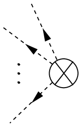
Figure 3: The tree-level potential and the counterterms include vertices depending only on $X^{+}$ (depicted here by dashed, oriented lines).

The connected loop diagrams consist strictly of a closed solid line with dashed lines emanating from an arbitrary number of points on the solid line. This is depicted for the four-point interaction in Fig. 4. This classification exhausts the set of connected Feynman diagrams in the theory. In particular, every connected correlator is exact at one loop.

Figure 4: The four-point Feynman diagram, exact at one-loop order.

2.5 Dynamical readjustment of the metric and dilaton gradient

The one-loop diagrams can be thought of as a set of effective vertices for $X^{+}$, associated with integrating out the massive field $X_{2}$. The operators generated in this fashion redefine the background fields in the target space of the lower-dimensional string theory at large $X^{+}$. Most of these fields vanish in the limit $X^{+}\to\infty$. To see this, note that an operator with canonical weight $(h,h)$ can only appear dressed with $M^{1-h}$. For instance, the operator $(\partial_{-}X^{+})(\partial_{-}^{2}X^{+})(\partial_{-}^{3}X^{+})(\partial_{+}X^{+})(\partial_{+}^{2}X^{+})(\partial_{+}^{3}X^{+})$ can only acquire the dressing $\mu^{-10}\,{\rm exp}\left(-5\beta X^{+}\right)$. Since all undressed operators that appear have integer weight, the only operator with increasing dependence on $X^{+}$ is the identity, dressed with ${\rm exp}\left(\beta X^{+}\right)$. However, this is just the coupling of the lower-dimensional effective tachyon, which we have fine-tuned to zero by adjusting $\mu^{\prime 2}$.

Dressed operators of weight $(2,2)$ and higher die off with increasing $X^{+}$. Therefore, the only $2D$ couplings on which the loop diagrams have any effect in the $X^{+}\to\infty$ limit are the string frame metric $G_{\mu\nu}$, which couples to $(\partial_{+}X^{\mu})(\partial_{-}X^{\nu})$, and the dilaton $\Phi$, which couples to the worldsheet Ricci scalar. (Worldsheet parity symmetry, among other constraints, forbids a renormalized background for the $B_{\mu\nu}$ field in this solution).

It is not difficult to integrate out $X_{2}$ and extract the one-loop shifts in these two couplings. Integrating out a real scalar with mass $M$ contributes to the effective dilaton (see Ref. [2] for further details) by an amount

$$\Delta\Phi=+{1\over 6}\ln\left(\,{M\over{\tilde{\mu}}}\,\right)\ ,$$ (2.33)

where $\tilde{\mu}$ is an arbitrary mass scale involved in the definition of the path integral measure. Since $M\equiv\mu\,{\rm exp}\left({1\over 2}\beta X^{+}\right)$, this gives

$$\Delta\Phi=\left(\,{\rm const.}\,\right)+{\beta\over{12}}X^{+}\ .$$ (2.34)

There is also a nonzero renormalization of the string-frame metric. For a mass term ${1\over 2}M^{2}(X)~{}X_{2}^{2}$, where $M$ depends arbitrarily on all coordinates other than $X_{2}$, the metric $G_{\mu\nu}$ is renormalized [2] by an amount

$$\Delta G_{\mu\nu}=+{{{\alpha^{\prime}}{}}\over 6}{{\partial_{\mu}M\partial_{\nu}M}\over{M^{2}}}\ .$$ (2.35)

For $M=\mu\,{\rm exp}\left({1\over 2}\beta X^{+}\right)$, this gives

$$\Delta G_{++}=+{{{\alpha^{\prime}}{}\beta^{2}}\over{24}}\ ,$$ (2.36)

with all other components unrenormalized. The renormalized upper-indexed metric then reads

$$G^{--}=-{{{\alpha^{\prime}}{}\beta^{2}}\over{24}}\ ,$$ (2.37)

with all other upper-index metric components unrenormalized. The renormalization of the dilaton and metric is depicted diagrammatically in Fig. 5.

Figure 5: Diagrams contributing to the nonvanishing renormalizations of the dilaton and metric, $\Delta(\partial_{+}\Phi)$ and $\Delta G_{++}$.

Let us now check the linear dilaton contribution to the central charge in the $X^{+}\to\infty$ limit. From the above analysis, we find a renormalized dilaton gradient $\hat{V}_{\mu}\equiv V_{\mu}+(\Delta V)_{\mu}$ and string frame metric $\hat{G}_{\mu\nu}\equiv G_{\mu\nu}+\Delta G_{\mu\nu}$ given by

$$\hat{V}_{-}=V_{-}=-{q\over{\sqrt{2}}}\ ,$$

$$\hat{V}_{+}=-{q\over{\sqrt{2}}}+{\beta\over{12}}\ ,$$

$$\hat{G}^{+-}=\hat{G}^{-+}=-1\ ,\qquad\hat{G}^{--}=-{{{\alpha^{\prime}}{}\beta^{2}}\over{24}}\ ,\qquad\hat{G}^{++}=0\ .$$ (2.38)

In the limit $X^{+}\to+\infty$, we therefore recover a contribution to the central charge from the renormalization of the linear dilaton equal to

$$c^{\rm dilaton}=6{\alpha^{\prime}}{}\hat{G}^{\mu\nu}\hat{V}_{\mu}\hat{V}_{\nu}=-6{\alpha^{\prime}}{}q^{2}+{{q\beta{\alpha^{\prime}}{}}\over{\sqrt{2}}}-{{{\alpha^{\prime}}{}^{2}q^{2}\beta^{2}}\over 8}\ .$$ (2.39)

Using $q^{2}=(D-26)/6{\alpha^{\prime}}{}$ and $q\beta={{2\sqrt{2}}\over{{\alpha^{\prime}}{}}}$, we find, in the $X^{+}\to\infty$ limit,

$$c^{\rm dilaton}=6{\alpha^{\prime}}{}\hat{G}^{\mu\nu}\hat{V}_{\mu}\hat{V}_{\nu}=-(D-26)+1\ .$$ (2.40)

The central charge contribution from $X_{2}$ decreases by one unit in this limit, so the total central charge remains the same. Instead of an overall net change, units of central charge contribution have merely been transferred from those of the free scalar $X_{2}$ to those coming from the strength of the dilaton gradient. Henceforth, we refer to this effect as central charge transfer.

The central charge transfer mechanism works equally well when the tachyon has a quadratic minimum in several dimensions $X_{2},\cdots,X_{n+1}$, rather than just one. In that case, the worldsheet Lagrangian is deformed by a term $\Delta{\cal L}=-{1\over{2\pi}}{\cal T}(X)$, with

$${\cal T}(X)={{\mu^{2}}\over{2\,{\alpha^{\prime}}{}}}~{}{\rm exp}\left(\beta X^{+}\right)~{}\sum_{i=2}^{n+1}\,:X_{i}^{2}:+{\cal T}_{0}(X^{+})\ ,$$

$${\cal T}_{0}(X^{+})={{n\,\mu^{2}\,X^{+}}\over{{\alpha^{\prime}}{}\,q\,\sqrt{2}}}\,{\rm exp}\left(\beta X^{+}\right)+\mu^{\prime 2}\,{\rm exp}\left(\beta X^{+}\right)\ .$$ (2.41)

The renormalizations of $\hat{G}^{\mu\nu}$ and $\hat{V}_{\mu}$ receive contributions from $n$ real scalars, rather than just one:

$$\hat{V}_{-}=-{q\over{\sqrt{2}}}\ ,\qquad\hat{V}_{+}=-{q\over{\sqrt{2}}}+{{n\beta}\over{12}}\ ,$$

$$\hat{G}^{+-}=\hat{G}^{-+}=-1\ ,\qquad\hat{G}^{--}=-{{n{\alpha^{\prime}}{}\beta^{2}}\over{24}}\ ,\qquad\hat{G}^{++}=0\ .$$ (2.42)

The dilaton contribution to the central charge in the $X^{+}\to\infty$ limit becomes

$$c^{\rm dilaton}=6{\alpha^{\prime}}{}\hat{G}^{\mu\nu}\hat{V}_{\mu}\hat{V}_{\nu}=-6{\alpha^{\prime}}{}q^{2}+{{nq\beta{\alpha^{\prime}}{}}\over{\sqrt{2}}}-{{n{\alpha^{\prime}}{}^{2}q^{2}\beta^{2}}\over 8}=-(D-26)+n\ ,$$ (2.43)

which compensates the loss of $n$ units of central charge carried by the $n$ real scalars $X_{2},\cdots,X_{n+1}$.

The central charge transfer described here is the same as the mechanism studied in [2]. In the model studied in [2], the tachyon condenses along a timelike rather than lightlike direction. As a result, there are Feynman diagrams involving loops of the $X^{0}$ field that make contributions to the renormalized metric and dilaton, suppressed by powers of $n/(D-D_{\rm crit})$. The CFT describing timelike tachyon condensation can only be treated semiclassically if $D>>D_{\rm crit}$ and $n$ is small, so the description [2] can never be perturbative when describing a return to the critical vacuum. In the present model, the one-loop renormalizations are exact, and no large-$D$ limit need be taken. We can therefore study transitions in which the number of spacetime dimensions at $X^{+}\to\infty$ is equal to the critical dimension or less!

To make the final number of dimensions equal to the critical dimension $D_{\rm crit}=26$, choose $n=D-26$. The final dilaton gradient is nonvanishing, but it is null with respect to the final string-frame metric. Furthermore, the product $\hat{G}^{\mu\nu}\hat{V}_{\mu}{{\partial_{\nu}{\cal T}}/{{\cal T}}}$ is positive, signaling a dilaton rolling to infinitely weak coupling in the future of the final, critical vacuum.

In the remainder of this paper we study several models describing tachyon condensation along lightlike directions in type 0/type II and heterotic string theories. In each of the models we study, amplitudes receive quantum corrections from Feynman diagrams with at most one loop, and central charge is transferred from free fields to the strength of the dilaton gradient in such a way that the theories at $X^{+}=\pm\infty$ have the same total central charge, despite living in different numbers of spacetime dimensions.

3 Dimension-changing transitions in heterotic string theory

We will now describe exact classical solutions of heterotic string theory in which the total number of spacetime dimensions decreases by $n$. In the case $n=D-10$, the final vacuum has the critical number of dimensions $D_{\rm crit}=10$, with flat string-frame metric, and lightlike linear dilaton rolling to weak coupling in the future. The particular heterotic theory we study has gauge symmetry $SO(22+D)$ and a tachyon ${\cal T}^{a}$ transforming in the fundamental representation. This is the second of the two unstable heterotic theories described in [3], named type HO^+/. The tachyon in the type 0 theory has a single real component ${\cal T}$, as always.

If the $D$-dimensional theory at $X^{+}=-\infty$ has its spacelike dimensions in the form of the maximally Poincare-invariant $D-1$ dimensional ${\rm I\kern-1.79993ptR}^{D-1}$, then the final theory is type HO^+/ in $D-n$ dimensions, with spatial slices of the form ${\rm I\kern-1.79993ptR}^{D-1-n}$.

Alternately, the spatial slices of the initial theory can be given certain orbifold singularities on which light spacetime fermions can live. The lower-dimensional theory at $X^{+}=+\infty$ then has spacetime fermions as well. In the case where the final dimension is critical, we can reach the spacetime-supersymmetric $SO(32)$ heterotic theory.

In all cases, the readjustment of the dilaton and the string-frame metric comes from a one-loop calculation on the worldsheet, just as in the dimension-changing transition we studied in the bosonic string in the previous section.

3.1 Description of type HO^+/ string theory in $D>10$

In heterotic string theory, the local worldsheet gauge symmetry of the string is $(0,1)$ superconformal invariance. Let us focus immediately on the simplest heterotic string theory that can live in $D$ dimensions, type HO^+/. Not counting ghosts and superghosts, the degrees of freedom on the string worldsheet are $D$ embedding coordinates $X^{\mu}$, their right-moving fermionic superpartners $\psi^{\mu}$, and $D+22$ left-moving current algebra fermions $\tilde{\lambda}^{a}$. Physical states of the string correspond to normalizable states that are primary under the left-moving Virasoro algebra and the right-moving super-Virasoro algebra. Additionally, physical states must have weight $(1,{1\over 2})$.

The discrete gauge group of the worldsheet is a single, overall $\mathchoice{\hbox{\cmss Z\kern-3.99994ptZ}}{\hbox{\cmss Z\kern-3.99994ptZ}}{\lower 0.9pt\hbox{\cmsss Z\kern-2.79996ptZ}}{\lower 1.2pt\hbox{\cmsss Z\kern-2.79996ptZ}}_{2}$ that flips the sign on all fermions (both $\tilde{\lambda}^{a}$ and $\psi^{\mu}$) simultaneously. In other words, the partition function on the torus corresponds to the diagonal modular invariant. There is a single Ramond sector, in which the $\psi^{\mu}$ and $\tilde{\lambda}^{a}$ are simultaneously periodic. These states correspond to spacetime fermions that are spinors under $SO(D-1,1)$ and $SO(D+22)$. The ground-state energy in this sector is ${1\over{16}}(D+22)$: since all such states are heavy, we will focus only on NS states.

For consistency, the total central charge of the matter must be $(26,15)$. The central charge of $D$ free scalars along with $D$ right-moving and $D+22$ left-moving fermions is equal to $(26,15)+\left(\,{3\over 2}(D-10),{3\over 2}(D-10)\,\right)$. We can cancel the central charge excess by adding a dilaton gradient $V_{+}=V_{-}=-{q/{\sqrt{2}}}$, where $q^{2}={1\over{4{\alpha^{\prime}}{}}}(D-10)$. The central charge is then critical, and the worldsheet CFT defines a classical solution to string theory that comprises a heterotic version of the timelike linear dilaton theory. Conformal invariance is automatic, since the worldsheet theory is free and massless, with action

$${\cal L}_{\rm kin}={1\over{2\pi}}G_{\mu\nu}\left[\,{2\over{{\alpha^{\prime}}{}}}(\partial_{+}X^{\mu})(\partial_{-}X^{\nu})-i\psi^{\mu}(\partial_{-}\psi^{\nu})\,\right]-{i\over{2\pi}}\tilde{\lambda}^{a}(\partial_{+}\tilde{\lambda}^{a})\ .$$ (3.1)

3.2 Giving a vev to the tachyons ${\cal T}^{a}$

We can deform the timelike linear dilaton background by letting the tachyon acquire a nonzero value obeying the equations of motion. The tachyon transforms in the fundamental of $SO(D+22)$. A nonzero tachyon vev ${\cal T}^{a}(X)$ couples to the worldsheet as a superpotential

$$W\equiv\tilde{\lambda}^{a}:{\cal T}^{a}(X):\ ,$$ (3.2)

where the component action comes from integrating the superpotential over a single Grassmann direction $\theta_{+}$:

$${\Delta{\cal L}} \equiv -{1\over{2\pi}}\int d\theta_{+}~{}W$$ (3.3)

$$= -{1\over{2\pi}}\left(\,F^{a}:{\cal T}^{a}(X):-i\sqrt{{\alpha^{\prime}}{}\over 2}\,:\partial_{\mu}{\cal T}^{a}(X):\tilde{\lambda}^{a}\psi^{\mu}\,\right)\ .$$

The object $F^{a}$ is an auxiliary field, and the kinetic term for the free, massless theory contains a quadratic term ${1\over{2\pi}}F^{a}F^{a}.$ Integrating out $F^{a}$ results in a potential of the form

$$\Delta{\cal L}=-{1\over{8\pi}}\sum_{a}:{\cal T}^{a}(X)^{2}:\ ,$$ (3.4)

and a supersymmetry transformation $\{Q,\tilde{\lambda}^{a}\}=F^{a}={1\over 2}:{\cal T}^{a}:$.

The operator $:{\cal T}^{a}(X):$ must be a superconformal primary of weight $({1\over 2},{1\over 2})$. Therefore, the equation of motion for a weak tachyon field is

$$\partial^{\mu}\partial_{\mu}{\cal T}^{a}-2V^{\mu}\partial_{\mu}{\cal T}^{a}+{2\over{\alpha^{\prime}}{}}{\cal T}^{a}=0\ .$$ (3.5)

Even for perturbations satisfying the linearized equations of motion, there will generally be singularities in the product of a tachyon insertion with itself. Consequently, there will arise a nontrivial conformal perturbation theory that must be solved order by order in the strength of ${\cal T}^{a}$. However, there are special choices of ${\cal T}^{a}$ for which there are no singularities in the OPE of a superpotential insertion with itself, and the perturbation is exactly marginal.

The simplest such choice is for the gradient of the tachyon to lie in a lightlike direction:

$${\cal T}^{a}=\mu^{a}{\rm exp}\left(\beta X^{+}\right)\ ,$$ (3.6)

with $q\beta={{\sqrt{2}}\over{\alpha^{\prime}}{}}$. The resulting bosonic potential is positive-definite and increasing exponentially toward the future:

$$\Delta{\cal L}=-{1\over{8\pi}}(\mu^{a})^{2}~{}{\rm exp}\left(2\beta X^{+}\right)+{i\over{2\pi}}\sqrt{{\alpha^{\prime}}{}\over 2}\beta\mu^{a}{\rm exp}\left(\beta X^{+}\right)~{}\tilde{\lambda}^{a}\psi^{+}\ .$$ (3.7)

This theory has a potential barrier that is like a Liouville wall moving to the left at the speed of light, similar to the solution of [5]. This theory may have interesting dynamics, and should be studied further.

The next simplest case is the one in which we allow the tachyon to vary in $n$ dimensions $X_{2},\ldots,X_{n+1}$ transverse to the light-cone dimensions $X^{\pm}$. We assume that the tachyon has an isolated zero ${\cal T}^{1}=\cdots={\cal T}^{n}=0$ at $X_{2}=\cdots=X_{n+1}=0$, and we take the limit in which the spatial wavelengths $k_{2}^{-1},\cdots,k_{n+1}^{-1}$ of the tachyons go to infinity. We can then approximate the tachyon field by

$${\cal T}^{a}(X)=\sqrt{2\over{\alpha^{\prime}}{}}\,{\rm exp}\left(\beta X^{+}\right)\left[\,\sum_{b=1}^{n}\hat{\mu}^{a}{}_{b}~{}X_{b+1}+O\left(\,kX^{2}\,\right)\,\right]\ ,$$ (3.8)

with

$$q\beta={{\sqrt{2}}\over{\alpha^{\prime}}{}}\ .$$ (3.9)

Taking the long-wavelength limit for the tachyons amounts to dropping the $kX^{2}$ terms. The assumption of an isolated zero is equivalent to assuming $\hat{\mu}^{a}{}_{b}$ is nondegenerate. For simplicity, let $\hat{\mu}^{a}{}_{b}\equiv\mu~{}\delta^{a}_{b}$. The superpotential is then

$$W=+\mu\,\sqrt{2\over{\alpha^{\prime}}{}}~{}{\rm exp}\left(\beta X^{+}\right)\sum_{a=1}^{n}\tilde{\lambda}^{a}X_{a+1}\ ,$$ (3.10)

and the interaction Lagrangian appears as

$${\cal L}_{\rm int} = -{{\mu^{2}}\over{4\pi}}\,{\rm exp}\left(2\beta X^{+}\right)\,\sum_{a=1}^{n}:X_{a+1}^{2}:$$ (3.11)

$$+{{i\mu}\over{2\pi}}{\rm exp}\left(\beta X^{+}\right)\,\sum_{a=1}^{n}\tilde{\lambda}^{a}\left(\,\psi^{a+1}+\beta X_{a+1}\psi^{+}\,\right)\ .$$

This superpotential is the same as the one in [3, 2], except that the tachyon is increasing in a lightlike direction rather than a timelike direction.

The equations of motion are

$$\partial_{+}\partial_{-}X^{+} = \partial_{-}\psi^{+}=0\ ,$$

$$\partial_{+}\partial_{-}X^{i} = -{{\mu^{2}}\over 4}\,{\rm exp}\left(2\beta X^{+}\right)\,X^{i}\ ,\qquad i=2,\cdots,n+1\ ,$$

$$\partial_{+}\partial_{-}X^{-} = +{{\beta}\over 4}\,{\rm exp}\left(2\beta X^{+}\right)\,\biggl{(}\sum_{i=2}^{n+1}X_{i}X_{i}\biggr{)}$$

$$-{{i\beta{\alpha^{\prime}}{}}\over 4}\,{\rm exp}\left(\beta X^{+}\right)\,\sum_{a=1}^{n}\tilde{\lambda}^{a}\left(\,\psi^{a+1}+\beta\,X_{a+1}\psi^{+}\,\right)\ ,$$

$$\partial_{+}\tilde{\lambda}^{a} = {{\mu}\over 2}\,{\rm exp}\left(\beta X^{+}\right)\,\left(\,\psi^{a+1}+\beta X_{a+1}\psi^{+}\,\right)\ ,$$

$$\partial_{-}\psi^{i} = -{\mu\over 2}\,{\rm exp}\left(\beta X^{+}\right)\,\tilde{\lambda}^{i-1}\ ,\qquad i=2,\cdots,n+1\ ,$$

$$\partial_{-}\psi^{-} = {{\beta\mu}\over 2}{\rm exp}\left(\beta X^{+}\right)\,\sum_{a=1}^{n}\tilde{\lambda}^{a}X_{a+1}\ .$$ (3.12)

In infinite volume, the construction of the general classical solution proceeds in parallel with the case of the bosonic dimension-changing transition. If we are interested in understanding the classical behavior, we can set the fermions to zero. Defining $f_{\pm},~{}{\bf F}_{\pm}$ as in Eqns. (2.12) and (2.13), we write

$$X^{+}={1\over 2}f_{+}(\sigma^{+})+{1\over 2}f_{-}(\sigma^{-})\ .$$ (3.13)

The general solution for $X_{i}$ is then

$$X_{i}=\sum_{\omega}A_{\omega,(i)}\,{\rm exp}\left({i\over 2}\omega{\bf F}_{+}(\sigma^{+})+{i\over 2}{{\mu^{2}}\over\omega}{\bf F}_{-}(\sigma^{-})\right)\ .$$ (3.14)

Choosing a set of mode amplitudes $A_{\omega,(i)}$, one can solve the equations of motion for $X^{-}$ by treating it as Poisson’s equation, with a fixed source proportional to $\sum_{i}X_{i}^{2}\,{\rm exp}\left(2\beta X^{+}\right)$.

To understand the classical behavior of strings at late times, we make the ansatz $\partial_{\sigma^{1}}X^{+}=0,$ and define ${N}_{n(i)}(\sigma^{0})$ as the occupation numbers for the modes of the $X_{i}$ fields. Choosing $p^{+}>0$, we have

$$X^{+}={\alpha^{\prime}}{}p^{+}(\sigma^{0}-\sigma^{0}_{(0)})+X^{+}_{(0)}\ ,$$

$${N}_{n(i)}(\sigma^{0})\sim{N}_{n(i)}^{\rm(fin.)}\ ,$$ (3.15)

for large values of $X^{+}$. If we further assume that the $X_{i}$ are independent of $\sigma^{1}$, then ${N}_{i(n)}=0$ for $n\neq 0$. In this case the behavior of $X^{-}$ at late times approaches

$$X^{-}\sim\sum_{i}{{{N}_{0(i)}\,M(\sigma^{0})}\over{\beta{\alpha^{\prime}}{}p^{+2}R_{\rm ws}}}\ .$$ (3.16)

Any nonzero values for $N_{n(i)}$ ($n\neq 0$) can only contribute positively to the growth of $X^{-}$, by an amount increasing exponentially in time like $M$. A particle therefore accelerates to the left, quickly approaching the speed of light, unless all its $X_{i}$ oscillators are in their ground states.

The theory behaves in a simple fashion at the quantum level as well. Just as for the dimension-changing transition in the bosonic string, the renormalization of the dilaton and metric occur only at one-loop order on the worldsheet, where only the massive fields $\tilde{\lambda}^{a},~{}X_{a+1},~{}\psi^{a+1}$ circulate in the loop.

Integrating out a massive Majorana fermion of mass $M(X)$ gives the shifts

$$\Delta\Phi=+{1\over{12}}\ln\left(\,{M\over{\tilde{\mu}}}\,\right)\ ,\qquad\Delta G_{\mu\nu}=+{{{\alpha^{\prime}}{}}\over{12}}{{\partial_{\mu}M\partial_{\nu}M}\over{M^{2}}}\ ,$$ (3.17)

at one-loop order. Here, $M(X)$ is allowed to depend arbitrarily on the target space coordinates $X^{\mu}\in\{X^{\pm},X_{n+2},\cdots,X_{D-1}\}$, which are not being integrated out. Using the formulae in Eqns. (2.33) and (2.35), we see that the contribution from the massive boson is twice that for the massive fermion. The total contribution from all the massive $X,~{}\psi$ and $\tilde{\lambda}$ fields is therefore

$$\Delta\Phi=+{n\over{4}}\ln\left(\,{M\over{\tilde{\mu}}}\,\right)\ ,\qquad\Delta G_{\mu\nu}=+{n\over{4}}{{\partial_{\mu}M\partial_{\nu}M}\over{M^{2}}}\ .$$ (3.18)

Letting

$$M\equiv\mu\,{\rm exp}\left(\beta X^{+}\right)\ ,$$ (3.19)

we obtain

$$\Delta V_{+}=+{{n\beta}\over{4}}\ ,\qquad\Delta G_{++}=+{{n\beta^{2}{\alpha^{\prime}}{}}\over{4}}\ ,\qquad\Delta G^{--}=-{{n\beta^{2}{\alpha^{\prime}}{}}\over{4}}\ ,$$ (3.20)

with all other components of $G_{\mu\nu}$ and $V_{\mu}$ unrenormalized.

One difference from the dimension-changing domain wall in the bosonic string is that the potential energy need not be fine-tuned by hand. Since we are integrating out fields in complete multiplets, the quantum correction to the potential energy vanishes. Even nonperturbatively, the effective potential at $X_{2}=\cdots=X_{n+1}=0$ must vanish. Any correction to the effective potential must come from an effective superpotential term containing a single $\tilde{\lambda}$ fermion. The remaining fermions are $\tilde{\lambda}^{n+1},\cdots,\tilde{\lambda}^{D+22}$. Any effective superpotential with a single $\tilde{\lambda}$ fermion would violate the residual $SO(D+22-n)$ symmetry left unbroken by the tachyon vev.

The linear dilaton central charge at $X^{+}\to+\infty$ is

$$c^{\rm dilaton}=6{\alpha^{\prime}}{}\hat{G}^{\mu\nu}\hat{V}_{\mu}\hat{V}_{\nu}=-6{\alpha^{\prime}}{}q^{2}+{{3nq\beta{\alpha^{\prime}}{}}\over{\sqrt{2}}}-{{3n\beta^{2}q^{2}{\alpha^{\prime}}{}^{2}}\over 4}\ .$$ (3.21)

Using $q^{2}={1\over{4{\alpha^{\prime}}{}}}(D-10)$ and $q\beta=\sqrt{2}/{\alpha^{\prime}}{}$, we find that the final dilaton central charge is

$$c^{\rm dilaton}={3\over 2}\left[\,-(D-10)+n\,\right]\ .$$ (3.22)

Thus, exactly ${{3n}/2}$ units of central charge are transferred from the $n$ massless multiplets $X_{a+1},~{}\psi^{a+1}$ and current algebra fermions $\tilde{\lambda}^{a}$ to the dilaton gradient at $X^{+}=+\infty$. The total central charge is again the same at $X^{+}=+\infty$ as at $X^{+}=-\infty$, and in particular equal to $(26,15)$.

3.3 Transitions among nonsupersymmetric heterotic theories

In the case where the spatial slices are simply ${\rm I\kern-1.79993ptR}^{D-1}$, we can choose $n$ to be any integer from $1$ to $D-2$. We always end up at $X^{+}=+\infty$ with a consistent string theory in $D-n$ dimensions with total central charge equal to $(26,15)$. If $n<D-10$, the final theory is another supercritical theory. If $n>D-10$, we end up with a subcritical theory with a spacelike linear dilaton. In both cases there is a tachyon in the fundamental representation of the unbroken gauge group $SO(D+22-n)$. If $n=D-10$, our final theory is a critical, unstable heterotic string theory with gauge group $SO(32)$ and a lightlike linear dilaton rolling to weak coupling in the future. The spacetime transition from $D$ to $D-n$ dimensions is depicted schematically in Fig. 6.

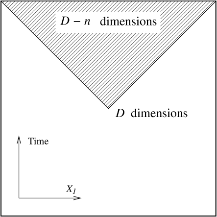
Figure 6: The dynamical transition from $D$ dimensions outside a bubble wall to $D-n$ dimensions in the interior. Our solution focuses on the upper left-hand corner of the diagram, where the bubble is a domain wall moving to the left at the speed of light.

We can also choose the maximal number of transverse dimensions $n=D-2$. In this case, the tachyon in the final theory is stabilized due to its modified dispersion relation in the background of the linear dilaton [17]. This theory has unbroken gauge symmetry $SO(24)$, and a finite number of local degrees of freedom (namely, a set of scalar tachyons in the fundamental representation of $SO(24)$).

In other words, the tachyon in the $2D$ string theory is precisely zero. The end of the throat in the $2D$ theory is at infinitely strong coupling, with no Liouville wall to bar string states from the strong coupling region; this theory was studied in [18]. At a generic point in the moduli space of the $2D$ theory, the tachyon condensate is nonzero, and the maximum coupling attainable by a string is finite. This perturbation cuts off the strong coupling end of the theory with a Liouville wall, and is a valid perturbation of the pure $2D$ string theory. However, we do not know how this perturbation may lift to a deformation of our full solution.

The $2D$ heterotic background was analyzed recently in [19, 20] and found to have a nontrivial phase structure, as well as a characteristic nonlocal behavior not familiar from field theory or other string theories. It would be interesting to understand the ways in which the peculiar properties of the $2D$ heterotic theory might descend from the properties of the higher dimensional theory that from which it decays via closed string tachyon condensation.

3.4 Return to the supersymmetric vacuum in $D=10$ with gauge group $SO(32)$

Another interesting option is to orbifold the spatial slices ${\rm I\kern-1.79993ptR}^{D-1}$ by a $\mathchoice{\hbox{\cmss Z\kern-3.99994ptZ}}{\hbox{\cmss Z\kern-3.99994ptZ}}{\lower 0.9pt\hbox{\cmsss Z\kern-2.79996ptZ}}{\lower 1.2pt\hbox{\cmsss Z\kern-2.79996ptZ}}_{2}$ involution that acts on $D-10$ of the spatial coordinates $X_{2},\ldots,X_{D-9}$, leaving only $9$ spatial dimensions and the time dimension unorbifolded. Modular invariance constrains the action of the involution on current algebra fermions $\tilde{\lambda}^{a}$. The simplest modular invariant choice is to act with a $-1$ on all $D+22$ of the $\tilde{\lambda}^{a}$. This singularity was studied in [3] and referred to as an orbifold singularity of stable type.

This choice preserves the full $SO(D+22)$ gauge symmetry, and leaves massless fermions propagating on the $9+1$-dimensional fixed locus of the $\mathchoice{\hbox{\cmss Z\kern-3.99994ptZ}}{\hbox{\cmss Z\kern-3.99994ptZ}}{\lower 0.9pt\hbox{\cmsss Z\kern-2.79996ptZ}}{\lower 1.2pt\hbox{\cmsss Z\kern-2.79996ptZ}}_{2}$ reflection. The localized massless spectrum includes a spacetime fermion transforming as a massless spin-${3\over 2}$ field under the 9+1 dimensional longitudinal Poincare group. The orbifold projection imposes a boundary condition forcing the tachyons ${\cal T}^{a}$ to vanish at the fixed locus.

Upon perturbing the system with a tachyon vev

$${\cal T}^{a}(X)=\sqrt{2\over{\alpha^{\prime}}{}}\,\hat{\mu}^{a}{}_{b}~{}{\rm exp}\left(\beta X^{+}\right)~{}X_{b+1}\ ,$$ (3.23)

one needs the superpotential to be even under the orbifold action. We may therefore use only odd coordinates $X_{b+1},~{}b\in\{1,\cdots,D-10\}$. The mass matrix $\hat{\mu}$ thus has rank $n$ at most $D-10$, and we will take it to be $\mu\,\mathbbm{1}_{\rm n\times n}.$

The maximal value $n=D-10$ is particularly interesting. In this case, the final theory is critical, with lightlike linear dilaton and continuous gauge group $SO(32)$. The GSO projection inherited by the critical theory is $\mathchoice{\hbox{\cmss Z\kern-3.99994ptZ}}{\hbox{\cmss Z\kern-3.99994ptZ}}{\lower 0.9pt\hbox{\cmsss Z\kern-2.79996ptZ}}{\lower 1.2pt\hbox{\cmsss Z\kern-2.79996ptZ}}_{2}\times\mathchoice{\hbox{\cmss Z\kern-3.99994ptZ}}{\hbox{\cmss Z\kern-3.99994ptZ}}{\lower 0.9pt\hbox{\cmsss Z\kern-2.79996ptZ}}{\lower 1.2pt\hbox{\cmsss Z\kern-2.79996ptZ}}_{2}$, generated by worldsheet fermion number mod two, $g_{\rm F}\equiv(-1)^{F_{W}}$ and $g_{\rm L}\equiv(-1)^{\#\tilde{\lambda}}$, which is the center of the unbroken $SO(32)$. The bosons and right-moving fermions on which $g_{\rm L}$ acts nontrivially are massive, and decoupled at $X^{+}\to+\infty$. Likewise, after we integrate out massive fields at $X^{+}\to+\infty$, $g_{\rm R}\equiv g_{\rm F}g_{\rm L}$ acts only on right-moving fermions $\psi^{\mu}$. The $\mathchoice{\hbox{\cmss Z\kern-3.99994ptZ}}{\hbox{\cmss Z\kern-3.99994ptZ}}{\lower 0.9pt\hbox{\cmsss Z\kern-2.79996ptZ}}{\lower 1.2pt\hbox{\cmsss Z\kern-2.79996ptZ}}_{2}\times\mathchoice{\hbox{\cmss Z\kern-3.99994ptZ}}{\hbox{\cmss Z\kern-3.99994ptZ}}{\lower 0.9pt\hbox{\cmsss Z\kern-2.79996ptZ}}{\lower 1.2pt\hbox{\cmsss Z\kern-2.79996ptZ}}_{2}$ GSO projection is precisely the spacetime-supersymmetric GSO projection of the $SO(32)$ heterotic string. The gravitini that generate spacetime supersymmetry transformations are the massless ground states of the sector twisted by $g_{\rm R}$.

The final state of our theory is therefore a state of the supersymmetric heterotic string with $SO(32)$ gauge group. Indeed, the final state in this example is actually a BPS solution in the limit $X^{+}\to\infty$. To see this, recall the supersymmetry transformations for the heterotic string [21]

$$\delta\Psi_{\mu} = \left[\,\nabla_{\mu}+{1\over 4}\omega_{\mu}^{A}{}_{B}\Gamma_{A}{}^{B}-{1\over 4}H_{\mu\nu\sigma}\Gamma^{\nu\sigma}\,\right]\epsilon\ ,$$

$$\delta\Lambda = \left[\,\Gamma^{\mu}(\nabla_{\mu}\Phi)-{1\over 6}H_{\mu\nu\sigma}\Gamma^{\mu\nu\sigma}\,\right]\epsilon\ ,$$

$$\delta\chi^{[ab]} = F_{\mu\nu}^{[ab]}\Gamma^{\mu\nu}\epsilon\ .$$ (3.24)

For flat string-frame metric, vanishing $H$-flux and trivial $SO(32)$ gauge field, the supersymmetry transformations reduce to

$$\delta\Psi_{\mu}=\partial_{\mu}\epsilon\ ,\qquad\delta\Lambda=\Gamma^{\mu}(\partial_{\mu}\Phi)\epsilon\ ,\qquad\delta\chi^{[ab]}=0\ .$$ (3.25)

For a lightlike linear dilaton, the matrix $\Gamma^{\mu}(\partial_{\mu}\Phi)$ is nilpotent of order $2$, and annihilates one half of the spinors on which it acts. The kernel can be taken to be constant spinors, so the gravitino variation vanishes. The gaugino variations vanish trivially, since the gauge field strength is turned off.

The late-time behavior of the solution is that of a state preserving 8 of 16 supersymmetries. We have found an exact solution connecting supercritical heterotic string theory in $D>10$ dimensions with a half-BPS state of the critical, 10-dimensional $SO(32)$ heterotic string theory.

4 Dimension-changing transitions in type 0 string theory

We can also study transitions from supercritical type 0 string theory to type 0 or type II string theory in lower dimensions. As in the heterotic case, starting with ${\rm I\kern-1.79993ptR}^{D-1}$ spatial slices gives rise to an unstable theory in lower dimensions. By starting with orbifolded spatial slices, it is possible to reach a final state that is spacetime supersymmetric.

The local worldsheet gauge symmetry in type 0 string theory is $(1,1)$ superconformal invariance. Not counting ghosts and superghosts, the $2D$ fields on the string worldsheet are $D$ embedding coordinates $X^{\mu}$ and their fermionic superpartners $\tilde{\psi}^{\mu},~{}\psi^{\mu}$, and the physical states of the string are normalizable, super-Virasoro primaries of weight $({1\over 2},{1\over 2})$. The total central charge of the matter must be $(15,15)$, and the central charge contributed by $D$ free massless fields $X^{\mu}$ and their superpartners is $(15,15)+\left(\,{3\over 2}(D-10),{3\over 2}(D-10)\,\right)$. The central charge excess can be canceled by adding a dilaton gradient $V_{+}=V_{-}=-{q/{\sqrt{2}}}$, where

$$q^{2}={1\over{4{\alpha^{\prime}}{}}}(D-10)\ .$$ (4.1)

The worldsheet CFT then defines a supercritical type 0 string theory, with worldsheet action

$${\cal L}_{\rm kin}={1\over{2\pi}}G_{\mu\nu}\left[\,{2\over{{\alpha^{\prime}}{}}}(\partial_{+}X^{\mu})(\partial_{-}X^{\nu})-i\psi^{\mu}(\partial_{-}\psi^{\nu})-i\tilde{\psi}^{\mu}(\partial_{+}\tilde{\psi}^{\nu})\,\right]\ .$$ (4.2)

4.1 Description of type 0 string theory in $D>10$

The discrete gauge group of the worldsheet is a single, overall $\mathchoice{\hbox{\cmss Z\kern-3.99994ptZ}}{\hbox{\cmss Z\kern-3.99994ptZ}}{\lower 0.9pt\hbox{\cmsss Z\kern-2.79996ptZ}}{\lower 1.2pt\hbox{\cmsss Z\kern-2.79996ptZ}}_{2}$ acting with a $-1$ simultaneously on all fermions $\psi,~{}\tilde{\psi}$. This is just the symmetry $(-1)^{\rm F_{\rm w}}$ of worldsheet fermion number mod 2, which must be gauged in any consistent theory involving worldsheet fermions. There is also an apparent global symmetry acting on $\tilde{\psi}$ with a $-1$ and on $\psi$ with a $+1$. We call this symmetry ‘apparent’ because it is violated in type 0 string theory in odd dimensions, as will be demonstrated below. This symmetry, which we refer to as $(-1)^{\rm F_{\rm L_{\rm w}}}$ (the ‘L’ indicates “left”), has no analog in the physical spectrum of type II string theories because it is gauged; it becomes part of the GSO group, along with $(-1)^{\rm F_{\rm w}}$.

All type 0 theories have a single real tachyon ${\cal T}$, corresponding to the oscillator ground state of the NS/NS sector. The tachyon ${\cal T}$ couples to the string worldsheet as a superpotential, so it must be odd under $(-1)^{\rm F_{\rm L_{\rm w}}}$ if $(-1)^{\rm F_{\rm L_{\rm w}}}$ is indeed a symmetry. In addition to the NS/NS sector, there is a R/R sector in which the worldsheet fermions are all periodic, and states correspond to $p$-form fields. In even dimensions, the massless content of the R/R sector is either $[0]^{2}\oplus[2]^{2}\oplus\cdots\oplus[{D\over 2}-3]^{2}\oplus[{D\over 2}-1]^{1}$ or $[1]^{2}\oplus[3]^{2}\oplus\cdots\oplus[{D\over 2}-2]^{2}$, depending on the sign choice of the GSO projection. Here $[p]$ denotes a massless $p$-form potential, and the superscript denotes the multiplicity. In odd dimensions there is only one choice of GSO projection, and the spectrum of $p$-form fields is $[0]^{1}\oplus[1]^{1}\oplus[2]^{1}\oplus\cdots\oplus[{{D-3}\over 2}]^{1}$.

In odd dimensions the symmetry $(-1)^{\rm F_{\rm L_{\rm w}}}$ is anomalous as a global symmetry on the string worldsheet. There is no consistent assignment of transformations to spin fields for which the OPE preserves any chiral R-parity. To see this, notice that the R/R $p$-forms have vertex operators that are spin fields for an odd number of left-moving and an odd number of right-moving worldsheet fermions. Likewise, the OPE of two such spin fields closes on NS/NS fields with an odd number of left- and an odd number of right-moving worldsheet fermions. There are therefore nonvanishing three-point functions that would violate the $\mathchoice{\hbox{\cmss Z\kern-3.99994ptZ}}{\hbox{\cmss Z\kern-3.99994ptZ}}{\lower 0.9pt\hbox{\cmsss Z\kern-2.79996ptZ}}{\lower 1.2pt\hbox{\cmsss Z\kern-2.79996ptZ}}_{2}$ symmetry for any choice of action on the R/R form. An example would be the three-point function involving two R/R axions and a tachyon.

Since the tachyon is odd under $(-1)^{\rm F_{\rm L_{\rm w}}}$, the symmetry $(-1)^{\rm F_{\rm L_{\rm w}}}$ cannot extend as a $\mathchoice{\hbox{\cmss Z\kern-3.99994ptZ}}{\hbox{\cmss Z\kern-3.99994ptZ}}{\lower 0.9pt\hbox{\cmsss Z\kern-2.79996ptZ}}{\lower 1.2pt\hbox{\cmsss Z\kern-2.79996ptZ}}_{2}$ symmetry to act in a consistent way on the R/R scalar as well. One could try to extend $(-1)^{\rm F_{\rm L_{\rm w}}}$ to generate a $\mathchoice{\hbox{\cmss Z\kern-3.99994ptZ}}{\hbox{\cmss Z\kern-3.99994ptZ}}{\lower 0.9pt\hbox{\cmsss Z\kern-2.79996ptZ}}{\lower 1.2pt\hbox{\cmsss Z\kern-2.79996ptZ}}_{4}$ symmetry, but this would mean it would have to act on the R/R zero-form with eigenvalue $\pm i$. The complex conjugate of the R/R axion would then have to have the conjugate eigenvalue. Since the R/R axion is a real field, however, this is not possible.

Another way to see the absence of a conserved $(-1)^{\rm F_{\rm L_{\rm w}}}$ is to consider amplitudes on the torus, with the odd spin structure $(P,P)$ for the worldsheet fermions. In $D$ dimensions, this spin structure has $D$ zero modes for the right-moving fermions and $D$ zero modes for the left-moving fermions. There are therefore nonvanishing amplitudes with $D$ tachyon vertex operators inserted. If $D$ is odd, there is no way for the tachyon to be odd under a conserved $(-1)^{\rm F_{\rm L_{\rm w}}}$.

Since we gain our control over tachyon condensation in the type 0 theory by using the exact global symmetry $(-1)^{\rm F_{\rm L_{\rm w}}}$, we will focus on even dimensions $D=10+2K$. Though it is not in general possible to orbifold by $(-1)^{\rm F_{\rm L_{\rm w}}}$ (i.e., to treat it as part of the GSO group), it is always a good global symmetry of the worldsheet in even dimensions, and therefore an exact discrete gauge symmetry in spacetime. Any superpotential $W$ preserving $(-1)^{\rm F_{\rm L_{\rm w}}}$ must be odd under it, since the superspace measure $\int d\theta_{+}d\theta_{-}$ is also odd. $(-1)^{\rm F_{\rm L_{\rm w}}}$ is therefore a discrete $R$-parity, and its existence will allow us to constrain tachyon condensates in a natural way, without fine-tuning.

4.2 Giving a vev to the tachyon ${\cal T}$

We wish to deform the background by a tachyon expectation value that obeys the equations of motion. The tachyon couples to the worldsheet as a superpotential, integrated over one Grassmann variable $\theta_{\pm}$ of each chirality:

$$\Delta{\cal L} = {i\over{2\pi}}\int d\theta_{+}d\theta_{-}{\cal T}(X)$$ (4.3)

$$= -{1\over{2\pi}}\,\sqrt{{\alpha^{\prime}}{}\over 2}\,F^{\mu}:\partial_{\mu}{\cal T}(X):+{{i{\alpha^{\prime}}{}}\over{4\pi}}:\partial_{\mu}\partial_{\nu}{\cal T}(X):\tilde{\psi}^{\mu}\psi^{\nu}\ .$$

Including the ${1\over{2\pi}}F^{\mu}F_{\mu}$ term that comes along with the kinetic term, and integrating out the auxiliary field $F^{\mu}$, we find the resulting potential

$$-\Delta{\cal L}={{\alpha^{\prime}}{}\over{16\pi}}G^{\mu\nu}(:\partial_{\mu}{\cal T}(X):)(:\partial_{\nu}{\cal T}(X):)\ .$$ (4.4)

The condition for conformal invariance of the linearized perturbation is that $:{\cal T}(X):$ be primary of weight $({1\over 2},{1\over 2})$. This amounts to the condition

$$\partial^{2}{\cal T}-2(V\cdot\partial){\cal T}+{2\over{\alpha^{\prime}}{}}{\cal T}=0\ .$$ (4.5)

Our exactly solvable examples have ${\cal T}$ appearing with exponential dependence on a lightlike direction. The simplest case to consider is the case where ${\cal T}={\rm exp}\left(\beta X^{+}\right)$ and $\beta q=\sqrt{2}/{\alpha^{\prime}}{}$. This perturbation is conformally invariant and gives rise to an exactly solvable background describing a transition between two different string theories. It does not reduce the number of spacetime dimensions, but instead changes the kind of string theory altogether. We describe this solution in detail in a separate paper [22].

Searching for exactly solvable models of dynamical dimension change, it turns out that the easiest models to control are those for which the vev of the tachyon preserves some spacetime reflection symmetry, combined with the chiral $R$-parity $(-1)^{\rm F_{\rm L_{\rm w}}}$. We thus look for perturbations such that the superpotential $W$ is odd under the reflection of some subset of the coordinates $Y^{b}\equiv X_{b+1},$ with $b=1,\ldots,~{}n$:

$${\cal T}=\sum_{b=1}^{n}:{{\tilde{f}_{b}(X)}\over{k_{b}}}\,\sin{(k_{b}Y^{b})}:\ ,$$ (4.6)

were the $\tilde{f}_{b}$ depend only on $X_{0},~{}X_{1},~{}X_{n+2},\ldots,~{}X_{D-1}$. Taking $k_{a}\to 0$, we obtain the limiting configuration

$${\cal T}=\sum_{b=1}^{n}:\tilde{f}_{b}(X)Y^{b}:\ .$$ (4.7)

We can further restrict the form of $\tilde{f}_{b}$ by adopting the following ansatz:

$$\tilde{f}_{b}\equiv{\rm exp}\left(\beta_{b}X^{+}\right)\,:f_{b}(X):\ ,$$ (4.8)

where $f_{b}(X)$ depends only on $X_{n+2},\ldots,~{}X_{D-1}$.

Treating the worldsheet dynamics semiclassically, the potential takes the form

$$-2\pi\,\Delta{\cal L} = \sum_{b=1}^{n}{\rm exp}\left(2\beta_{b}X^{+}\right)f_{b}(X)^{2}$$ (4.9)

$$+\sum_{a,b,c=1}^{n}{\rm exp}\left((\beta_{a}+\beta_{b})X^{+}\right)Y^{a}Y^{b}f_{a,c}(X)f_{b,c}(X)\ .$$

Let us analyze the classical supersymmetric moduli space of the worldsheet theory. Worldsheet supersymmetry is unbroken at exactly those values $X,~{}Y$ for which $\{f_{b}(X)=f_{b,c}(X)Y^{c}=0\}$. This contains the locus ${\bf M}\equiv\{f_{b}(X)=Y^{c}=0\}$. If ${\bf M}$ is a smooth manifold, then there are no other components. Some linear combinations of $Y^{c}$ can have classical flat directions over singular points in ${\bf M}$.

For a generic choice of functions $f_{b}(X)$, the space ${\bf M}$ will indeed be smooth. So the classical supersymmetric vacuum manifold at fixed $X^{0,1}$ defines a smooth submanifold of real codimension $n$ in the ${\rm I\kern-1.79993ptR}^{D-2-n}$-space spanned by $X_{n+2},\ldots,~{}X_{D-1}$. Treating the dynamics semiclassically, the theory at $X^{+}\to+\infty$ is a sigma model on ${\bf M}$, times ${\rm I\kern-1.79993ptR}^{1,1}$. To the extent that our semiclassical treatment signals the existence of a well-defined CFT, the full $2$D field theory, with $X^{\pm}$ included, describes a transition from type 0 string theory on ${\rm I\kern-1.79993ptR}^{D-1,1}$ to type 0 string theory on ${\rm I\kern-1.79993ptR}^{1,1}\times{\bf M}$, where the dimensionality of ${\bf M}$ is $D-2-2n$.

Such a CFT describes a transition in which the string theory begins in a primordial, cosmological state at early times and chooses a topology dynamically, through closed string tachyon condensation.

In general, worldsheet quantum effects on the worldsheet will alter this picture substantially. The on-shell condition for the linearized tachyon perturbation is

$$\partial^{2}{\cal T}-2V\cdot\partial{\cal T}+{2\over{\alpha^{\prime}}{}}{\cal T}=0\ ,$$ (4.10)

which is satisfied if and only if

$$\partial_{i}^{2}f_{b}(X)=-k_{b}^{2}f_{b}(X)\equiv\left(\,-{2\over{\alpha^{\prime}}{}}+\sqrt{2}\beta_{b}q\,\right)f_{b}(X)\ .$$ (4.11)

By superposing different $f_{b}$, tuning coefficients and taking the long-wavelength limit $k_{b}^{2}{\alpha^{\prime}}{}\to 0$, one can obtain superpotentials of the form ${\rm exp}\left(\beta X^{+}\right)~{}Y^{b}~{}{\bf P}_{b}(X_{i},X^{+})$, where ${\bf P}_{b}(X_{i},X^{+})$ are polynomials in the $X_{i}$ and $X^{+}$. At fixed $X^{+}$, the locus ${\bf M}$ is an arbitrary real algebraic variety. The $X^{+}$ encode the leading logarithmic corrections to the size and shape of the manifold ${\bf M}$ under renormalization group flow. The $X^{+}$ dependence of the shape can vanish only if $\partial_{i}^{2}{\bf P}_{b}=0$.

We consider the simplest case where the above condition holds, namely when the $f_{b}(X)$ are linear functions of $X$:

$$f_{b}(X)=\sum_{a=1}^{n}\hat{\mu}^{a}{}_{b}X_{n+1+a}\ .$$ (4.12)

The condition that ${\bf M}$ be nonsingular reduces to the condition that $\hat{\mu}^{a}{}_{b}$ have nonvanishing determinant. For simplicity, we take $\hat{\mu}$ equal to $\mu\,{\mathbbm{1}}_{{\rm n}\times{\rm n}}$:

$$\hat{\mu}^{a}{}_{b}\equiv\mu\,\delta^{a}{}_{b}\ ,$$ (4.13)

in which case the full superpotential is

$$W={\cal T}=\mu\,{\rm exp}\left(\beta X^{+}\right)\sum_{b=1}^{n}\,Y^{b}X_{n+1+b}\ ,\qquad q\beta={{\sqrt{2}}\over{\alpha^{\prime}}{}}\ .$$ (4.14)

This CFT is exactly solvable, both at the classical and at the quantum level. The analysis of the general classical solution on a noncompact worldsheet proceeds completely in parallel with the analysis of the dimension-changing transition in the bosonic string and the heterotic string. The fields $X^{+},~{}\psi^{+},$ and $\tilde{\psi}^{+}$ are free, and the massive fields $Y^{b}$ and $X_{n+1+b}$ (and their superpartners) obey free equations of motion with time-dependent mass terms, proportional to exponentials of $X^{+}$.

The study of the classical equations of motion works the same in this example as in the bosonic and heterotic examples. As in those cases, the classical potential is simply a number of scalar fields $X_{b+n+1},~{}Y^{b},$ with masses equal to $\mu\,{\rm exp}\left(\beta X^{+}\right)$. Taking the ansatz $\partial_{\sigma^{1}}X^{+}=0$, we can solve for the trajectories of the string in terms of Bessel functions, and we find exactly the same behavior as in the bosonic and heterotic cases: states of the string with massive fields excited have their energy locked permanently into the massive modes by virtue of the adiabatic theorem. They are then pushed along the bubble wall for the rest of time. States that have no massive modes excited can freely penetrate into the interior of the tachyonic phase, where they move in $2n$ fewer dimensions.

The simplifications at the quantum level that hold for the bosonic and heterotic worldsheet theories, hold in the CFT of this section as well. All connected tree and loop graphs consist of a single open or closed massive line, with lightlike lines emanating from some number of vertices placed along the line. In particular, the couplings that define the metric and dilaton receive corrections only from one-loop graphs, when the massive degrees of freedom are integrated out. The difference here is that the massive multiplets running in the loop are larger, containing the fields $X_{n+1+b},~{}Y^{b},~{}\psi^{X_{n+1+b}},~{}\psi^{Y^{b}},~{}\tilde{\psi}^{X_{n+1+b}}$ and $\tilde{\psi}^{Y^{b}}$ for all $b=1,\ldots,n$. The outgoing lines attached to the massive loop are all “$+$” lines, just as in the heterotic and bosonic examples. In the bosonic case there were only outgoing $X^{+}$ lines, while outgoing $\psi^{+}$ lines were also allowed in the heterotic case. In the type $0$ examples, outgoing lines attached to a loop include the fields $X^{+},~{}\psi^{+}$ and $\tilde{\psi}^{+}$.

In the case where the spatial slices are simply ${\rm I\kern-1.79993ptR}^{D-1}$, we can choose $n$ to be any integer in the range $n\in 1,\ldots,~{}{D\over 2}-1$. At $X^{+}=+\infty$ we arrive at a consistent string theory in $D-2n$ dimensions, with total central charge equal to $15$. If $2n<D-10$, the final theory is another supercritical theory, while for $2n>D-10$ we end up with a subcritical theory with a spacelike linear dilaton. If $2n=D-10$, the final theory is a critical, unstable string theory of type $0$ with a lightlike linear dilaton rolling to weak coupling in the future. This theory has an unbroken $\mathchoice{\hbox{\cmss Z\kern-3.99994ptZ}}{\hbox{\cmss Z\kern-3.99994ptZ}}{\lower 0.9pt\hbox{\cmsss Z\kern-2.79996ptZ}}{\lower 1.2pt\hbox{\cmsss Z\kern-2.79996ptZ}}_{2}$ symmetry under which the tachyon is odd. The tachyon in the $2D$ string theory is identically zero. The $2D$ type 0 theory can be deformed by the addition of a Liouville wall in the usual way [18]. As for the $2D$ heterotic case, we do not know what deformation of our full, time-dependent solution would produce a Liouville wall in the final state.

4.3 Return to the supersymmetric type II vacuum in $D=10$

We can also consider orbifolding the spatial slices in a particularly interesting way. As in the heterotic case, allowed orbifold singularities are highly constrained by the requirement of modular invariance, which manifests itself as the need for level matching in twisted sectors. For the type 0 string in $D\equiv 10+2K$ dimensions, the simplest consistent orbifold action is a $\mathchoice{\hbox{\cmss Z\kern-3.99994ptZ}}{\hbox{\cmss Z\kern-3.99994ptZ}}{\lower 0.9pt\hbox{\cmsss Z\kern-2.79996ptZ}}{\lower 1.2pt\hbox{\cmsss Z\kern-2.79996ptZ}}_{2}$ generated by an operation $g_{\rm L}$. We define $g_{\rm L}$ to act by reflection of the $K$ real coordinates $Y^{b}$, as well as acting by the symmetry $(-1)^{\rm F_{\rm L_{\rm w}}}$, which acts as $-1$ on the left-moving worldsheet supercurrent. In other words, in addition to its geometric action, $g_{\rm L}$ is a chiral $R$-parity. The full GSO/orbifold group is then $\{1,~{}(-1)^{\rm F_{\rm w}},~{}g_{\rm L},~{}g_{\rm R}\equiv(-1)^{\rm F_{\rm w}}\cdot g_{\rm L}\}$.

The resulting singularity $Y^{b}=0$ preserves a Poincare invariance of the ${\rm I\kern-1.79993ptR}^{9+K,1}$ longitudinal to the fixed locus, parametrized by $\{X^{0},~{}X_{1},~{}X_{K+2},\ldots,~{}X_{2K+9}\}$. This symmetry is broken only by the timelike linear dilaton. There is also an $SO(K)$ rotational invariance transverse to the fixed locus. In the NS/NS and R/R sectors the coordinates $Y^{b}$ are untwisted, while in the R/NS and NS/R sectors the coordinates $Y^{b}$ are twisted. That is, spacetime fermions live only on the geometric fixed locus, and spacetime bosons propagate only in the bulk.

Now we calculate the ground state weights in the various sectors, ignoring the contributions of $\psi^{0,1},~{}\tilde{\psi}^{0,1}$ fermions. The oscillator ground states in the R/NS sector have weight $\left({K\over 8}+{1\over 2},{K\over 8}\right)$. The GSO and orbifold projections in the twisted R/NS sector can be satisfied by acting with a single fermionic oscillator $\psi^{X^{\mu}}$, with $\mu=0,~{}1,~{}K+2,\ldots,~{}2K+9$, which gives a level-matched state of weight $\left(\,{K\over 8}+{1\over 2},{K\over 8}+{1\over 2}\,\right)$. The ground states in the twisted R/NS sector make up the states of a massless vector-spinor $\Psi^{\mu}_{\alpha p}$, where $\alpha$ is a spinor index of $SO(9+K,1)$ and $p$ is a spinor index of the transverse $SO(K)$. The vector index $\mu$ runs only along the longitudinal directions $\mu=0,~{}1,~{}K+2,\ldots,~{}2K+9$. The NS/R sector is also level-matched, with the same content as the R/NS sector.

The GSO projection cuts the multiplicity of the localized fermions by imposing the condition

$$\left(\,\Gamma_{\rm SO(9+K,1)}\otimes\gamma_{\rm SO(K)}\,\right)\cdot\Psi^{\mu}=\pm\Psi^{\mu}\ ,$$ (4.15)

where $\Gamma_{\rm SO(9+K,1)}$ and $\gamma_{\rm SO(K)}$ are products of all gamma matrices of the longitudinal $SO(9+K,1)$ and the transverse $SO(K)$, respectively. The $\pm$ sign can be chosen independently in the NS/R and R/NS sectors. When $K$ is even, these are simply the usual chirality matrices, up to a phase. When $K$ is odd, there is no chirality for spinors of $SO(9+K,1)$ or $SO(K)$, but there is still a combined condition that cuts the complex Dirac spinor representation by two. The precise meaning of this condition depends on the value of $K$, mod eight, and can be read off the table and discussion in Appendices A.3 and A.4 of [3] (with $n$ in that reference replaced by $K$ here.) There is also a reality condition naturally derived from the reality of the worldsheet fermions. The details of this condition also depend on the value of $K$ mod eight (for further details, the reader is referred to Ref. [3]).

Apart from generating an interesting spectrum of massless fermions propagating on the fixed locus, the other effect of the orbifolding is to impose boundary conditions on the bulk fields at the orbifold singularity $Y^{b}=0$. In particular, the superpotential $W$ must be odd under any chiral $R$-parity. If $W$ is a function of $X,~{}Y$ only, it must therefore be odd under $Y^{b}\to-Y^{b}$.

Since any allowed worldsheet superpotential must be odd under $g_{\rm L}$, the tachyon must be odd under reflection of $Y$:

$${\cal T}(X,-Y)=-{\cal T}(X,Y)\ .$$ (4.16)

In particular, the tachyon must vanish at the origin of the $Y$ coordinate. The bosonic potential must therefore have a minimum at $Y=0$ with zero energy, just as in the heterotic case.

By pairing $Y$ and $X$ coordinates with mass terms in the superpotential, we can eliminate a maximum of $2K$ dimensions: all $K$ of the $Y$ dimensions can pair with $K$ of the $X^{\mu}$ directions and give them mass. The minimum dimension of the final state is therefore the critical dimension $D_{\rm crit}=10$. By the same calculation we performed in the heterotic case (see Eqn. (3.22)), the metric and dilaton change by

$$\Delta V_{+}=+{{n\beta}\over{2}}\ ,\qquad\Delta G_{++}=+{{n\beta^{2}{\alpha^{\prime}}{}}\over{2}}\ ,\qquad\Delta G^{--}=-{{n\beta^{2}{\alpha^{\prime}}{}}\over{2}}\ .$$ (4.17)

The renormalized dilaton central charge is

$$c^{\rm dilaton}=3(n-K)\ .$$ (4.18)

When $n=K$, the final state has $10$ dimensions, the dilaton central charge vanishes and the readjusted dilaton is null with respect to the readjusted metric. Moreover, the GSO projection is that of type II string theory rather than type 0. Since all degrees of freedom in the $Y$ multiplets have become massive and decoupled, the orbifold symmetry $g_{\rm L}$ acts only on the remaining left-moving fermions $\tilde{\psi}^{\mu}$. That is, $g_{\rm L}$ becomes equal to $(-1)^{\rm F_{\rm L_{\rm w}}}$. Therefore the GSO group in the final state at $X^{+}\to\infty$ is generated by $(-1)^{\rm F_{\rm L_{\rm w}}}$ and $(-1)^{\rm F_{\rm w}}$, which means the effective GSO projection and Ramond sector content is exactly that of a type II string, rather than type 0 string. The final vacuum is the critical, supersymmetric vacuum of type II string theory, with the choice of IIA or IIB depending on whether the initial supercritical state is type 0A or 0B.

In the absence of flux and curvature, the supersymmetry transformations of the gravitini and dilatini in type II string theory are

$$\delta\Psi_{\mu}^{(1,2)}=\partial_{\mu}\epsilon^{(1,2)}\ ,\qquad\delta\Lambda^{(1,2)}=\Gamma^{\mu}(\partial_{\mu}\Phi)\epsilon^{(1,2)}\ .$$ (4.19)

For a final dilaton gradient $\partial_{\mu}\Phi$ that is constant and lightlike, there are exactly 16 supercharges preserved, out of the full 32. Our solution therefore describes the dynamical relaxation of a nonsupersymmetric, supercritical phase of string theory to a half-BPS state of the critical type II theory. In the case where the final state is type IIA string theory, other solutions with the same late-time asymptotics have been found [23], and defined nonperturbatively in the string coupling. The resolution of the early-time behavior is quite different from ours, involving a matrix theory definition of the strong coupling region rather than the addition of supercritical dimensions. There are, in other words, at least two valid completions of the the 10-dimensional lightlike linear dilaton theory in the strong coupling regime. This serves as a reminder of the dissipative nature of physics in an expanding universe.

5 Conclusions

We have introduced solutions to string theory that interpolate between theories in different total numbers of spacetime dimensions. These backgrounds are solutions to the classical equations of motion in the spacetime sense, and we have shown that they are exact to all orders, in the worldsheet sense. The consistency of these transitions depends on the dynamical readjustment of the dilaton and the metric. These effects come from a one-loop renormalization on the string worldsheet, and they render the total central charge on the worldsheet critical in both limits of the solution, $X^{+}\to\pm\infty$.

The solutions work similarly in the bosonic, type 0, and unstable heterotic HO^+/ theories. In the latter two cases, orbifold singularities can be introduced into the initial state, with boundary conditions chosen such that the final state can preserve some spacetime supersymmetry in the limit $X^{+}\to+\infty$. Since the spacetime supersymmetry of the final state is an exact symmetry of the dynamics, it must be viewed as broken spontaneously, rather than explicitly, for finite $X^{+}$. We arrive at the striking conclusion that string theories in arbitrarily high dimensions can preserve an exact dynamical supersymmetry, albeit nonlinearly realized. Our exact solutions describing transitions from the supercritical theory to supersymmetric vacua of the critical theory provide conclusive evidence in favor of the proposals in [3, 2].

We have shown that our CFT can be solved exactly at the classical level, on a worldsheet of infinite extent. It seems unlikely that quantum corrections should vitiate the solvability of the classical theory, since the perturbation series in all of our models terminate at one loop. Solving the theories explicitly in finite volume, and with quantum corrections included, would be extremely interesting.

The total number of string states at a given mass level goes down when the number of spacetime dimensions decreases. Even with our simple ansatz for classical solutions of the worldsheet theory, we can see the outlines of the mechanism by which the number of degrees of freedom in the theory is reduced. String states that do not ‘fit’ into the worldsheet CFT of the final spacetime are pushed along the wall of an expanding bubble. Only string states with no degrees of freedom excited in the massive sectors are allowed to enter the interior of the tachyonic phase.

We also saw that the final state of the theory, including the topology and total number of dimensions, is not dictated by the initial state. Rather, it is determined dynamically by the configuration of the closed string tachyon. This suggests a picture of a string landscape in which all lower-lying regions are accessible from a summit of highly supercritical theories. The notion of the supercritical string as a primordial phase from which all other string theories can emerge can be viewed as a closed-string extension of the $K$-theory constructions of open string theory [27]. We feel this direction of investigation deserves further development.

References

- [1] C. Aragone and S. Deser, “CONSISTENCY PROBLEMS OF HYPERGRAVITY,” Phys. Lett. B86 (1979) 161.
- [2] S. Hellerman and X. Liu, “Dynamical dimension change in supercritical string theory,” hep-th/0409071.
- [3] S. Hellerman, “On the landscape of superstring theory in ,” hep-th/0405041.
- [4] D. Z. Freedman, M. Headrick, and A. Lawrence, “On closed string tachyon dynamics,” Phys. Rev. D73 (2006) 066015, hep-th/0510126.
- [5] S. Hellerman and I. Swanson, “Cosmological solutions of supercritical string theory,” hep-th/0611317.
- [6] A. A. Tseytlin, “String vacuum backgrounds with covariantly constant null Killing vector and 2-d quantum gravity,” Nucl. Phys. B390 (1993) 153–172, hep-th/9209023.
- [7] A. A. Tseytlin, “Finite sigma models and exact string solutions with Minkowski signature metric,” Phys. Rev. D47 (1993) 3421–3429, hep-th/9211061.
- [8] G. T. Horowitz, “Tachyon condensation and black strings,” JHEP 08 (2005) 091, hep-th/0506166.
- [9] S. Hirano, “Energy quantisation in bulk bouncing tachyon,” JHEP 07 (2005) 017, hep-th/0502199.
- [10] M. Headrick, S. Minwalla, and T. Takayanagi, “Closed string tachyon condensation: An overview,” Class. Quant. Grav. 21 (2004) S1539–S1565, hep-th/0405064.
- [11] M. Gutperle, “A note on perturbative and nonperturbative instabilities of twisted circles,” Phys. Lett. B545 (2002) 379–383, hep-th/0207131.
- [12] R. Emparan and M. Gutperle, “From p-branes to fluxbranes and back,” JHEP 12 (2001) 023, hep-th/0111177.
- [13] M. S. Costa and M. Gutperle, “The Kaluza-Klein Melvin solution in M-theory,” JHEP 03 (2001) 027, hep-th/0012072.
- [14] A. Adams, X. Liu, J. McGreevy, A. Saltman, and E. Silverstein, “Things fall apart: Topology change from winding tachyons,” JHEP 10 (2005) 033, hep-th/0502021.
- [15] O. Aharony, M. Fabinger, G. T. Horowitz, and E. Silverstein, “Clean time-dependent string backgrounds from bubble baths,” JHEP 07 (2002) 007, hep-th/0204158.
- [16] V. Fateev, A. Zamolodchikov, and A. Zamolodchikov. Unpublished.
- [17] N. Seiberg, “Notes on quantum Liouville theory and quantum gravity,” Prog. Theor. Phys. Suppl. 102 (1990) 319–349.
- [18] M. R. Douglas et al., “A new hat for the matrix model,” hep-th/0307195.
- [19] J. L. Davis, F. Larsen, and N. Seiberg, “Heterotic strings in two dimensions and new stringy phase transitions,” JHEP 08 (2005) 035, hep-th/0505081.
- [20] N. Seiberg, “Long strings, anomaly cancellation, phase transitions, T- duality and locality in the 2d heterotic string,” JHEP 01 (2006) 057, hep-th/0511220.
- [21] C. G. Callan, Jr., J. A. Harvey, and A. Strominger, “Supersymmetric string solitons,” hep-th/9112030.
- [22] S. Hellerman and I. Swanson, “Cosmological unification of string theories,” hep-th/0612116.
- [23] B. Craps, S. Sethi, and E. P. Verlinde, “A matrix big bang,” JHEP 10 (2005) 005, hep-th/0506180.
- [24] H. Kodama and N. Ohta, “Time-dependent supersymmetric solutions in M theory and compactification - decompactification transition,” Prog. Theor. Phys. 116 (2006) 295–318, hep-th/0605179.
- [25] T. Ishino and N. Ohta, “Matrix string description of cosmic singularities in a class of time-dependent solutions,” Phys. Lett. B638 (2006) 105–109, hep-th/0603215.
- [26] T. Ishino, H. Kodama, and N. Ohta, “Time-dependent solutions with null Killing spinor in M- theory and superstrings,” Phys. Lett. B631 (2005) 68–73, hep-th/0509173.
- [27] E. Witten, “D-branes and K-theory,” JHEP 12 (1998) 019, hep-th/9810188.