Split String Formalism and the Closed String Vacuum, II

Theodore Erler
Harish-Chandra Research Institute
Chhatnag Road, Jhunsi, Allahabad 211019, India

E-mail:terler@mri.ernet.in

Abstract

In this paper we consider a class of generalizations of Schnabl’s solution of open bosonic string field theory obtained by replacing the wedge state by an arbitrary combination of wedge states. We find that under a few modest conditions such generalizations give a sensible deformation of Schnabl’s solution for the closed string vacuum—in particular, we can compute their energies and show that they reproduce the value predicted by Sen’s conjecture. Though these solutions are apparently gauge equivalent, they are not in general related by midpoint-preserving reparameterizations.

1 Introduction

Since Schnabl constructed his analytic solution of open bosonic string field theory (OSFT)[1], it has become possible to imagine that OSFT is a background independent framework which could allow exact computations of the properties of vacua in string theory (see ref.[2] for related important developments). Given this new solution, it is important to explore deformations in the hope of clarifying its structure and generating new solutions. As discussed in a previous paper[3](henceforth, (I)), the split string formalism[4, 5, 6] proves immensely useful in this capacity. One generalization suggested by this approach involves a choice of projector and its associated conformal frame[3, 7, 8]; these new solutions are related to Schnabl’s by midpoint preserving reparameterizations[8].

The split string formalism suggests a second interesting generalization[6]: Replace the wedge states separating the operator insertions in Schnabl’s solution by general sums of wedge states. In this paper we consider these solutions and the delicate limiting process required to calculate their energies. With the properly defined limit and some fortuitous cancellations, we are able to demonstrate the existence of an infinite class of new exact solutions describing the closed string vacuum. These solutions can be partitioned into families labeled by a wedge state $\Omega^{\gamma}$, interpolating between “identity based” solutions $\gamma=0$ and “sliver based” solutions $\gamma=\infty$. The solutions are apparently gauge equivalent, but are not in general related by reparameterizations.

This paper is organized as follows. In section 2 we review the split string formulation of Schnabl’s solution and explain the constraints on the wedge state combinations necessary to get nontrivial and well-defined solutions. In section 3 we evaluate the energy of these solutions and show that they reproduce the correct D-brane tension. In section 4 we show that the perturbative spectrum around these solutions is empty, along the lines of refs.[10, 11]. We end with some conclusions.

2 Setup

Let us quickly review the construction of Schnabl’s solution in the split string formalism[6, 3]. In this paper, all of the solutions we are interested in take the form,

$$\Psi=Fc\frac{KB}{1-F^{2}}cF$$ (2.1)

where $F,K,B,c$ are string fields and all products above are open string star products. In general $F$ can be any function of $K$,

$$F=F(K)$$

and the fields $K,B,c$ satisfy the simple properties,

$$Bc+cB=1\ \ \ \ \ \ \ \ KB-BK=0\ \ \ \ \ \ \ \ B^{2}=c^{2}=0$$ (2.2)

$$\ \ \ dK=0\ \ \ \ \ \ \ \ \ \ \ \ \ \ \ \ dB=K\ \ \ \ \ \ \ \ \ \ \ \ \ \ dc=cKc$$

where $d=Q_{B}$ is the BRST operator. A short calculation then shows that $\Psi$ satisfies the equations of motion:

$$d\Psi+\Psi^{2}=0$$ (2.3)

To get Schnabl’s original solution, we must make some additional choices in the definitions of $F,K,B$ and $c$. As explained in (I), an explicit realization of the identities eq.(2.2) is equivalent to the choice of a projector and its associated conformal frame (see also [7, 8]). Schnabl’s solution is formulated in the sliver frame, where explicitly

$$K = \frac{\pi}{2}(K_{1})_{L}|I\rangle\ \ \ \ \ K_{1}=L_{1}+L_{-1}$$

$$B = \frac{\pi}{2}(B_{1})_{L}|I\rangle\ \ \ \ \ B_{1}=b_{1}+b_{-1}$$

$$c = \frac{1}{\pi}c(1)|I\rangle$$ (2.4)

$|I\rangle$ is the identity string field and the subscript $L$ denotes taking the left half of the corresponding charge (integrating the current clockwise on only the positive half of the semicircle). For definiteness, we will focus on solutions in the sliver frame—at any rate, the energy calculation in the next section proceeds identically regardless of the choice of projector. To get Schnabl’s solution we must also make a particular choice for $F$:

$$F=e^{K/2}=\Omega^{1/2}$$ (2.5)

where $\Omega^{1/2}$ is the square root of the $SL(2,\mathbb{R})$ vacuum.

As discussed in (I) and ref.[8], we may generalize Schnabl’s solution by allowing $F$ to be an arbitrary wedge state,

$$F=e^{\gamma K/2}=\Omega^{\gamma/2}$$ (2.6)

for $\gamma\in[0,\infty]$. In the conformal field theory picture, this corresponds to “magnifying” the strips inside the cylindrical correlators defining Schnabl’s solution. We will call these pure wedge solutions; they are all related by a simple midpoint preserving reparameterization.

In this paper we consider composite wedge solutions, i.e. solutions where $F$ is allowed to be a more-or-less arbitrary function of $K$. To be specific, we will assume $F$ can be written as a kind of “Laplace transform,”

$$F=\Omega_{f}\equiv\int_{-\infty}^{\infty}dtf(t)\Omega^{t}$$ (2.7)

where $f$ is a real function, subject to a few conditions which we will explain shortly. Pure wedge solutions are a special case with,

$$f(t)=\delta\left(t-\frac{\gamma}{2}\right)$$ (2.8)

The fields $\Omega_{f}$ satisfy some nice properties:

$$\Omega_{f}\Omega_{g}=\Omega_{f\star g}\ \ \ \Omega_{f}+\Omega_{g}=\Omega_{f+g}$$ (2.9)

where $f\star g$ is the convolution product:

$$f\star g(t)=\int_{-\infty}^{\infty}dsf(t-s)g(s)$$ (2.10)

The identity of the convolution is a delta function, $1_{\star}=\delta(t)$.

The solution eq.(2.1) can be rewritten,

$$\Psi=\Omega_{f}cKB\Omega_{\left(\frac{1}{1-f^{2}}\right)_{\star}}c\Omega_{f}$$ (2.11)

where all the function products in the subscript are calculated with convolution. This is basically a shorthand notation for a triple integral over states of the form,

$$\Omega^{s}cKB\Omega^{t}c\Omega^{u}$$ (2.12)

In conformal field theory language, these states can be defined in terms of correlation functions on the cylinder $C_{s+t+u+1}$ with particular insertions. The cylinder is a strip in the complex plane $-\frac{1}{2}<\Re(z)<s+t+u+\frac{1}{2}$ with its boundaries identified; the local coordinate occupies the region $-\frac{1}{2}<\Re(z)<\frac{1}{2}$ and is the image of the unit disk under the sliver conformal map,

$$f_{\mathcal{S}}(z)=\frac{2}{\pi}\tan^{-1}z$$ (2.13)

Explicitly, eq.(2.12) is defined via the correlator,

$$\langle\Omega^{s}cKB\Omega^{t}c\Omega^{u},\chi\rangle=\left\langle c\left(t+u+\frac{1}{2}\right)KBc\left(u+\frac{1}{2}\right)f_{\mathcal{S}}\circ\chi(0)\right\rangle_{C_{s+t+u+1}}$$ (2.14)

where $K,B$ are the contour insertions,

$$K=\int_{i\infty}^{-i\infty}\frac{dz}{2\pi i}T(z)\ \ \ \ B=\int_{i\infty}^{-i\infty}\frac{dz}{2\pi i}b(z)$$ (2.15)

to be integrated between the two $c$ ghosts (see figure 2.1).

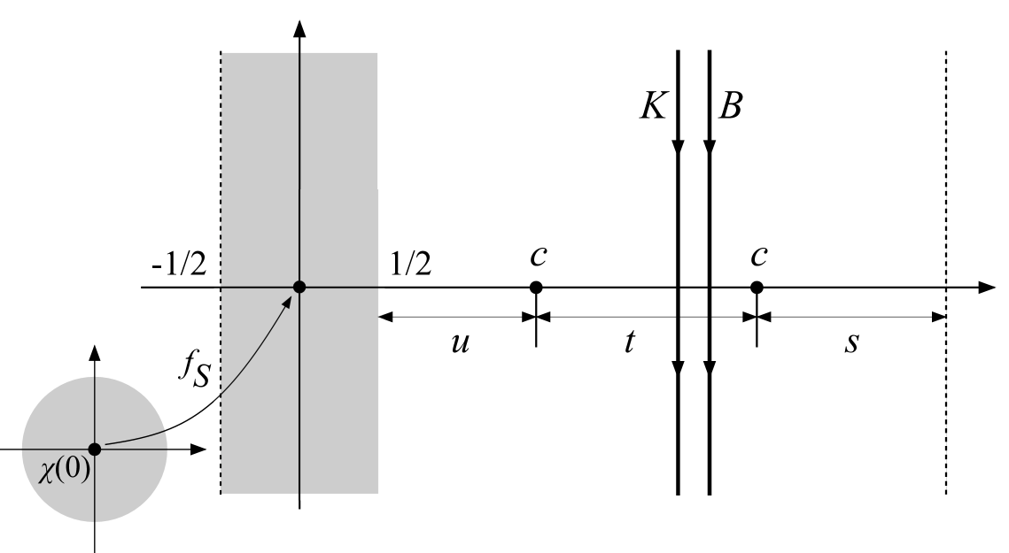
Figure 2.1: Conformal field theory representation of the state $\Omega^{s}cKB\Omega^{t}c\Omega^{u}$.

Let us now state the conditions which must be imposed on defining function $f(t)$:

$$\mathbf{(i)} \ \ f(t)=0\ \mathrm{for}\ t<0$$

$$\mathbf{(ii)} \ \ \int_{-\infty}^{\infty}dtf(t)=\sqrt{\lambda}=1$$

$$\mathbf{(iii)} \ \ \int_{-\infty}^{\infty}dt\,tf(t)=\frac{\gamma}{2}>0$$ (2.16)

Condition (i) follows from general considerations, specifically that the solution must not involve inverse wedge states. If such states exist, they are singular and best avoided. Condition (ii), as we will see, implies that the solution produces the energy of a single D-brane, in accordance with Sen’s conjectures. The constant $\lambda$ above is analogous to the parameter $\lambda$ labeling the pure gauge solutions studied by Schnabl[1]. For $\lambda<1$ the solutions are pure gauge; for $\lambda>1$ they are ill-defined; and for $\lambda=1$ they describe the closed string vacuum. The parameter $\gamma$ in condition (iii) is the exact counterpart of $\gamma$ in eq.(2.6); thus, composite wedge solutions can be partitioned into families labeled by a representative pure wedge solution. The restriction $\gamma>0$ follows from (i) in the pure wedge case, though we are not sure if it is necessary in general. We assume it is true for good measure.

Let us express the conditions (ii),(iii) in a few other convenient forms. Defining the square of $f(t)$,

$$w(t)\equiv f\star f(t)$$ (2.17)

conditions (ii), (iii) imply,

$$\int dtw(t)=\lambda=1\ \ \ \int dt\,tw(t)=\gamma$$ (2.18)

It is also useful to introduce the Fourier transform of $w(t)$:

$$w(t)=\int\frac{dx}{2\pi}W(x)e^{itx}$$ (2.19)

(ii) and (iii) are then re-expressed as:

$$W(0)=1\ \ \ W^{\prime}(0)=-i\gamma$$ (2.20)

Note that convolution products of $w(t)$ are isomorphic to local products of $W(x)$.

To calculate the energy, it is necessary to regulate the solutions eq.(2.11). Following Schnabl[1], we rewrite them in the form,

$$\Psi=\lim_{N\to\infty}\left(\sum_{n=0}^{N}\psi_{n}^{\prime}-\psi_{N}\right)$$ (2.21)

where,

$$\psi_{n}^{\prime}=FcBKF^{2n}cF\ \ \ \ \ \psi_{n}=\frac{1}{\gamma}FcBF^{2n}cF$$ (2.22)

This is a truncated Taylor expansion of eq.(2.11), modulo the $\psi_{N}$ piece which vanishes when contracted with Fock space states[1, 6, 9]. The factor of $1/\gamma$ in front of of $\psi_{n}$ is important. Though it is absent for Schnabl’s solution ($\gamma=1$) it is necessary to get the right energy from pure wedge solutions, and composite wedge solutions in general. Note that generally $\psi_{n}^{\prime}\neq\frac{d}{dn}\psi_{n}$, though this is the case for pure wedge solutions.

Let us explain briefly why the $\psi_{N}$ term in eq.(2.21) vanishes in the Fock space when $N\to\infty$. First, note that the infinite power of any $F$ satisfying (i)-(iii) gives the sliver state:

$$\lim_{N\to\infty}F^{N}=\Omega^{\infty}$$ (2.23)

This can be readily established using a trick which we explain in the next section. Next, consider the limit

$$\lim_{N\to\infty}KF^{N}=K\Omega^{\infty}=\left.\frac{d}{d\alpha}\Omega^{\alpha}\right|_{\alpha=\infty}=0$$ (2.24)

This vanishes since when $\alpha\to\infty$ the wedge state approaches a constant independent of $\alpha$ (the sliver). In fact, an explicit computation in the level expansion reveals that $\frac{d}{d\alpha}\Omega^{\alpha}$ vanishes as $1/\alpha^{3}$. Since from the perspective of commutation with the Virasoro generators the field $K$ is interchangeable with $B$, we may also conclude,

$$\lim_{N\to\infty}BF^{N}=0$$ (2.25)

Star multiplication with $FcF$ in both sides does not change this result. Therefore, $\psi_{N}$ vanishes in the large $N$ limit.

3 Energy

Now let us calculate the energy. Assuming the equations of motion, the action evaluated on eq.(2.21) takes the form,

$$S(\Psi)=-\frac{1}{6}\langle\Psi,Q_{B}\Psi\rangle=-\frac{1}{6}\left(\mathcal{K}_{0}-2\mathcal{K}_{1}+\mathcal{K}_{2}\right)$$ (3.1)

where,

$$\mathcal{K}_{0} = \lim_{N\to\infty}\langle\psi_{N},Q_{B}\psi_{N}\rangle$$

$$\mathcal{K}_{1} = \lim_{N\to\infty}\sum_{m=0}^{N}\langle\psi_{N},Q_{B}\psi_{m}^{\prime}\rangle$$

$$\mathcal{K}_{2} = \lim_{N\to\infty}\sum_{m,n=0}^{N}\langle\psi_{m}^{\prime},Q_{B}\psi_{n}^{\prime}\rangle$$ (3.2)

$$= \lim_{N\to\infty}\sum_{m=1}^{N}\sum_{n=N-m+1}^{N}\langle\psi_{m}^{\prime},Q_{B}\psi_{n}^{\prime}\rangle$$

In the second line of the third equation we have used,

$$\sum_{k=0}^{n}\langle\psi^{\prime}_{n-k},Q_{B}\psi_{k}^{\prime}\rangle=0$$ (3.3)

to cancel off the “lower half triangle” of the double sum. In (I) this equation was shown to hold for arbitrary choice of $F$. To prove Sen’s conjecture[12], we must demonstrate

$$E=-S(\Psi)=-\frac{1}{2\pi^{2}}$$ (3.4)

in the appropriate units.

The important consequence of eq.(3.3) is that we only need to calculate BRST inner products of the $\psi_{n}$s when $m+n$ is large—of order $N$. Let us consider:

$$\langle\psi_{m},Q_{B}\psi_{n}\rangle = \frac{1}{\gamma^{2}}\int d^{3}td^{3}s\left[f(t_{1})f^{\star 2m}(t_{2})f(t_{3})\right]\left[f(s_{1})f^{\star 2n}(s_{2})f(s_{3})\right]$$ (3.5)

$$\ \ \ \ \ \ \ \ \ \ \ \ \ \ \ \ \ \ \ \ \ \ \ \ \ \times\mathrm{Tr}\left[\Omega^{t_{1}}cB\Omega^{t_{2}}c\Omega^{t_{3}}d(\Omega^{s_{1}}cB\Omega^{s_{2}}c\Omega^{s_{3}})\right]$$

Here we use “split string” notation $\mathrm{Tr}[AB]=\langle A,B\rangle$; $f^{\star m}$ is the $m$th power of $f$ calculated with the convolution product. A little manipulation brings this into the form,

$$\langle\psi_{m},Q_{B}\psi_{n}\rangle=\frac{1}{\gamma^{2}}\int dsdt\,dSdT\,[w(s)w(S)^{\star m}][w(t)w(T)^{\star n}]C(s,S,t,T)$$ (3.6)

where,

$$C(s,S,t,T)=\mathrm{Tr}\left[\Omega^{s}cB\Omega^{S}c\Omega^{t}d(cB\Omega^{T}c)\right]$$ (3.7)

This quantity can be calculated as a correlation function on the cylinder; the full expression is complicated, but fortunately we will not need it.

Let us now consider the limit $m+n\to\infty$ of eq.(3.6). This limit of course is related to the limit $N\to\infty$ in eq.(3.2)—that is, $m$ and $n$ are typically of order $N$. We make this explicit by defining,

$$m=aN\ \ \ \ n=bN$$ (3.8)

The other ingredient we need is a substitution of variables in the integrand eq.(3.6):

$$S=N\sigma\ \ \ \ T=N\tau$$ (3.9)

We then want to calculate,

$$\lim_{N\to\infty}\langle\psi_{m},Q_{B}\psi_{n}\rangle=\frac{1}{\gamma^{2}}\lim_{N\to\infty}\int(dsdt)\,(d\sigma d\tau)\,w(s)w(t)[Nw(N\sigma)^{\star aN}][Nw(N\tau)^{\star bN}]C(s,N\sigma,t,N\tau)$$ (3.10)

To make sense of this, we need to understand the limit,

$$\lim_{N\to\infty}Nw(N\sigma)^{\star aN}$$ (3.11)

This expression is more transparent if we Fourier transform to “position space” $w(t)\to W(x)$:

$$Nw(N\sigma)^{\star aN}=\int\frac{dx}{2\pi}W\left(\frac{x}{N}\right)^{aN}e^{i\sigma x}$$ (3.12)

Thus the limit becomes,

$$\lim_{N\to\infty}W\left(\frac{x}{N}\right)^{aN}$$ (3.13)

Now note that, as a result of (ii) and (iii), $W$ has a Taylor expansion,

$$W(x)=1-i\gamma x+...$$ (3.14)

Plugging this in, the limit converges to an exponential:

$$\lim_{N\to\infty}W\left(\frac{x}{N}\right)^{aN}=e^{-i\gamma ax}$$ (3.15)

or,

$$\lim_{N\to\infty}Nw(N\sigma)^{\star aN}=\delta(\sigma-a\gamma)$$ (3.16)

Thus, as far as this factor is concerned, in the large $N$ limit the function $w$ is indistinguishable from a pure wedge solution!

Eq.(3.10) now simplifies to,

$$\lim_{N\to\infty}\langle\psi_{m},Q_{B}\psi_{n}\rangle=\frac{1}{\gamma^{2}}\lim_{N\to\infty}\int dsdt\,w(s)w(t)\,C(s,N\gamma a,t,N\gamma b)$$ (3.17)

To proceed we need some information about the function $C$. In appendix A we evaluate $C$ in the large $N$ limit by calculating the relevant correlator. The result is,

$$\lim_{N\to\infty}C(s,N\gamma a,t,N\gamma b)=st\mathcal{F}_{K}(a,b)$$ (3.18)

where $\mathcal{F}_{K}$ is the function introduced in ref.[6],

$$\mathcal{F}_{K}(a,b)=\frac{1}{\pi^{2}}\left(1+\cos\frac{\pi(a-b)}{a+b}\right)+\frac{2ab}{(a+b)^{2}}\cos\frac{\pi(a-b)}{a+b}+\frac{1}{\pi}\frac{a-b}{a+b}\sin\frac{\pi(a-b)}{a+b}$$ (3.19)

It is crucial that the dependence on $s$ and $t$ appears only in the factor $st$ in the large $N$ limit. In particular, we can calculate

$$\lim_{N\to\infty}\langle\psi_{m},Q_{B}\psi_{n}\rangle=\frac{1}{\gamma^{2}}\mathcal{F}_{K}(a,b)\int dsdt\,stw(s)w(t)=\frac{1}{\gamma^{2}}\mathcal{F}_{K}(a,b)\gamma^{2}$$ (3.20)

or,

$$\lim_{N\to\infty}\langle\psi_{m},Q_{B}\psi_{n}\rangle=\mathcal{F}_{K}(a,b)$$ (3.21)

This is exactly the result calculated for Schnabl’s solution. If anything other than the factor $st$ had appeared in $\lim_{N\to\infty}C$, the factors of $\gamma$ would not have canceled and the solutions would violate Sen’s conjecture. Note that pure wedge solutions would have been consistent with a more general quadratic dependence of $s,t$, so this is a nontrivial check on the consistency of these solutions.

Now consider the inner product,

$$\langle\psi_{m},Q_{B}\psi_{n}^{\prime}\rangle=\frac{1}{\gamma}\int dsdt\,dSdT\,[w(s)w(S)^{\star m}][w(t)w(T)^{\star n}]\frac{d}{dT}C(s,S,t,T)$$ (3.22)

Making the substitutions eqs.(3.8,3.9) we may compute the large $N$ limit:

$$\lim_{N\to\infty}\langle\psi_{m},Q_{B}\psi_{n}^{\prime}\rangle = \frac{1}{\gamma}\lim_{N\to\infty}\frac{1}{N}\int(dsdt)(d\sigma d\tau)\,w(s)w(t)[Nw(N\sigma)^{\star aN}][Nw(N\tau)^{\star bN}]\frac{\partial}{\partial\tau}C(s,N\sigma,t,N\tau)$$ (3.23)

$$= \frac{1}{\gamma}\lim_{N\to\infty}\frac{1}{N}\int(dsdt)(d\sigma d\tau)\,w(s)w(t)\delta(\sigma-a\gamma)\delta(\tau-b\gamma)\frac{\partial}{\partial\tau}C(s,N\sigma,t,N\tau)$$

$$= \frac{1}{\gamma}\lim_{N\to\infty}\frac{1}{N}\frac{\partial}{\partial(\gamma b)}\mathcal{F}_{K}(a,b)\int dsdt\,stw(s)w(t)$$

$$= \lim_{N\to\infty}\frac{1}{N}\frac{\partial}{\partial b}\mathcal{F}_{K}(a,b)$$

Again, the factors of $\gamma$ cancel out and we get the same result as for Schnabl’s solution. A similar argument shows,

$$\lim_{N\to\infty}\langle\psi_{m}^{\prime},Q_{B}\psi_{n}^{\prime}\rangle=\lim_{N\to\infty}\frac{1}{N^{2}}\frac{\partial}{\partial a}\frac{\partial}{\partial b}\mathcal{F}_{K}(a,b)$$ (3.24)

Calculation of the energy now proceeds exactly as it does for Schnabl’s solution[1, 6, 9]. The factors of $1/N,1/N^{2}$ turn the sums over $\psi_{n}^{\prime}$ in $\mathcal{K}_{1},\mathcal{K}_{2}$ into Riemann integrals over $a,b$. Thus,

$$E = \frac{1}{6}(\mathcal{K}_{0}-2\mathcal{K}_{1}+\mathcal{K}_{2})$$ (3.25)

$$= \frac{1}{6}\left(\mathcal{F}_{K}(1,1)+2\int_{0}^{1}db\frac{d}{db}\mathcal{F}_{K}(1,b)+\int_{0}^{1}da\int_{1-y}^{1}db\frac{\partial}{\partial a}\frac{\partial}{\partial b}\mathcal{F}_{K}(a,b)\right)$$

$$= \frac{1}{6}\left[\left(\frac{2}{\pi^{2}}+\frac{1}{2}\right)-2\left(\frac{2}{\pi^{2}}+\frac{1}{2}\right)+\left(-\frac{1}{\pi^{2}}+\frac{1}{2}\right)\right]$$

$$= -\frac{1}{2\pi^{2}}$$

Therefore, provided $f(t)$ satisfies conditions (i), (ii), and (iii), composite wedge solutions all describe the endpoint of tachyon condensation, i.e. the closed string vacuum. Following the discussion of refs.[6, 9] we can also show that the equations of motion are still satisfied when contracted with the solutions themselves.

4 Cohomology

An acceptable solution for vacuum must satisfy one other important constraint: its linearized fluctuations should support no physical open string excitations. For composite wedge solutions, the proof of this is simple and worth demonstrating. We must argue that the shifted BRST operator,

$$d_{\Psi}=d+[\Psi,\cdot]$$ (4.1)

has vanishing cohomology. Following refs.[10, 11], this follows if we can construct a field $A$ (the “homotopy operator”) such that

$$d_{\Psi}A=1$$ (4.2)

We now suppose that $A$ can be found within the subalgebra generated by $K,B$ and $c$. Since $A$ has ghost number $-1$, its form is fixed to be:

$$A=BG(K),$$ (4.3)

where $G$ is some field which depends only on $K$. For the moment it is sufficient to consider the unregularized solution, eq.(2.1); we compute,

$$d_{\Psi}A=KG+FcB\frac{F}{1-F^{2}}KG+KG\frac{F}{1-F^{2}}BcF$$ (4.4)

If we want the $B$s and $c$s to cancel, we should define $G$ so that it satisfies,

$$KG=1-F^{2}$$ (4.5)

Plugging this in,

$$d_{\Psi}A=1-F^{2}+F(cB+Bc)F=1$$ (4.6)

proving that $d_{\Psi}$ has no cohomology.

This proof assumes that eq.(4.5) has a solution for $G$ which yields a well-defined homotopy operator. To check this, let us solve eq.(4.5) explicitly. Writing $G$ in the form,

$$G=\int_{-\infty}^{\infty}dtg(t)\Omega^{t}$$ (4.7)

we can compute,

$$KG = \int_{-\infty}^{\infty}dtg(t)\frac{d}{dt}\Omega^{t}$$ (4.8)

$$= g(\infty)\Omega^{\infty}-\int_{-\infty}^{\infty}dt\frac{d}{dt}g(t)\Omega^{t}$$

$$= 1-F^{2}$$

Since $1-F^{2}$ has no term proportional to the sliver, we can only find a solution if $g(t)$ vanishes at infinity:

$$g(\infty)=0$$ (4.9)

Eq.(4.5) now becomes a differential equation for $g(t)$:

$$\frac{d}{dt}g(t)=w(t)-\delta(t)$$ (4.10)

Integrating,

$$g(t)=\left\{\begin{matrix}0\ \ \ \ \ &\mathrm{for}\ t<0\\ \displaystyle{-1+\int_{0}^{t}ds\,w(s)}\ \ \ &\mathrm{for}\ t>0\end{matrix}\right.$$ (4.11)

Consistency demands that this expression vanish at infinity,

$$g(\infty)=-1+\int_{0}^{\infty}ds\,w(s)=-1+\lambda=0$$ (4.12)

This is precisely condition (ii) needed to get nontrivial energy out of our solutions. Therefore, the homotopy operator $A$ exists, and the physical spectrum is empty, only for those solutions whose energies match that of a decayed D-brane. For Schnabl’s solution $w(t)=\delta(t-1)$ the homotopy operator takes the form,

$$A=-B\int_{0}^{1}dt\Omega^{t}$$ (4.13)

in agreement with the result of Ellwood and Schnabl[11].

For simplicity, in the above discussion we have used the unregularized solution and ignored possible terms, like the $\psi_{N}$ piece, which vanish in the Fock space. We are uncertain how such terms would effect the cohomology if present, but at any rate a quick calculation with the regularized solution eq.(2.21) and our expression for $G$ eq.(4.11) reveals that $d_{\Psi}A=1$ even outside the Fock space, as was demonstrated for the case of Schnabl’s solution in ref.[11]. Actually, this is less of a stringent consistency check than a resolution to an ambiguity in the definition of $A$ outside the Fock space; in particular, eq.(4.5) only determines the homotopy operator up to a term proportional to the sliver,

$$A=B(G+u\Omega^{\infty})$$ (4.14)

since the sliver is annihilated by $K$ and does not contribute to eq.(4.5). If we require $d_{\Psi}A=1$ even up to such “vanishing terms,” the undetermined constant $u$ is fixed to be zero and eq.(4.11) still gives the full solution for the homotopy operator.

5 Conclusion

In this paper we have constructed an infinite class of distinct and nontrivial descriptions of the closed string vacuum. It would be interesting to use these solutions to try to better understand the nature of open string gauge symmetry—specifically, to understand which gauge transformations are allowed and which are not allowed, and for what reasons. Recall that, at least naively, all the split string solutions eq.(2.1) are gauge equivalent to $\Psi=0$. However, apparently only a subset of the gauge transformations preserving conditions (i), (ii), and (iii) are actually valid.

We have not attempted a computation of the energies of these solutions in level truncation, though such calculations would be interesting. It seems likely that the convergence of the energy will vary widely depending on the choice of $f(t)$. For example, consider

$$f(t) = \delta(t)-\frac{1}{2}\delta^{\prime}(t)$$

$$F = 1+\frac{1}{2}K$$ (5.1)

This is an identity based solution whose energy is probably not very convergent in level truncation. Still it satisfies (i) (marginally), (ii), and (iii)—in fact, from the perspective of our analytic calculation, eq.(5.1) is in the same class as Schnabl’s solution with $\gamma=1$. It is also worth pointing out that condition (i), while it seems necessary, does not appear to play a role in the evaluation of the energy. Probably the hitch here is eq.(3.3), which allowed us to cancel off the $\psi_{n}$ inner products for small $m+n$. For solutions which violate or only marginally satisfy (i), the $\psi_{n}$ inner products for small $m+n$ are not very well defined, so eq.(3.3) should be treated with some suspicion. The other question is the necessity of condition (iii). If the other conditions are satisfied, it seems the energy calculation goes unchanged—$\gamma$ cancels out even if it is negative. Our only concern is that for $\gamma<0$, the function $C$ is formally an inner product of inverse wedge states. However, the analytic continuation to $\gamma<0$ appears fine, so these solutions could be okay after all.

To us, it is highly surprising that Schnabl’s regularization eq.(2.21) remains valid for composite wedge solutions. In some sense the regularization is “unnatural,” since each $\psi_{n}$ is composed of wedge states of all sizes. It would be interesting to understand this regulator better, or to discover other ways of regulating the solutions and calculating their energies.

The author would like to thank A. Sen for thoughtful conversations. This work was supported by the Department of Atomic Energy, Government of India.

Appendix A Correlator

In this appendix we would like to evaluate eq.(3.7),

$$C(s,aN,t,bN)=\mathrm{Tr}\left[\Omega^{s}cB\Omega^{aN}c\Omega^{t}d(cB\Omega^{bN}c)\right]$$ (A.1)

in the large $N$ limit. This quantity can be calculated as a correlation function on the cylinder, as shown in figure A.1

$$C(s,aN,t,bN)=\left\langle c(t+s+N(b+a))Bc(t+s+Nb)\left(\oint\frac{dz}{2\pi i}j_{B}(z)c(s+Nb)Bc(s)\right)\right\rangle_{C_{t+s+N(b+a)}}$$ (A.2)

The BRST current encircles all operators in the large parentheses, and (as usual) the $B$ contours pass between the $c$ ghosts on either side. Calculating the BRST variation and moving around some $B$ contours, this can be reduced to a sum of five terms:

$$C=X_{1}+X_{2}+X_{3}+X_{4}+X_{5}$$ (A.3)

where,

$$X_{1} = \langle c(t+s+N(a+b))c(t+s+Nb)c\partial c(s+Nb)B\rangle_{C_{t+s+N(b+a)}}$$

$$X_{2} = -\langle c(t+s+Nb)c\partial c(s+Nb)Bc(s)\rangle_{C_{t+s+N(b+a)}}$$

$$X_{3} = -\langle c(t+s+N(b+a))Bc(t+s+Nb)c(s+Nb)Kc(s)\rangle_{C_{t+s+N(b+a)}}$$

$$X_{4} = \langle c(t+s+N(b+a))Bc(s+Nb)c\partial c(s)\rangle_{C_{t+s+N(b+a)}}$$

$$X_{5} = -\langle c(t+s+N(b+a))Bc(t+s+Nb)c\partial c(s)\rangle_{C_{t+s+N(b+a)}}$$ (A.4)

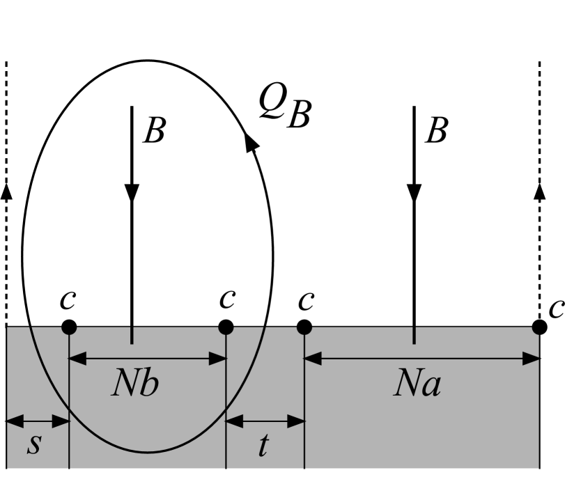
Figure A.1: Correlation function defining $C(s,Na,t,Nb)$.

Let us now concentrate on $X_{1}$. To understand the $N\to\infty$ limit it is helpful to scale the correlator by $1/N$. Scaling produces a factor of $N$ for each $c$, no factor for $\partial c$, and a factor of $1/N$ for the $B$ contour. All in all, $X_{1}$ becomes,

$$X_{1}=N^{2}\left\langle c\left(a+b+\frac{s+t}{N}\right)c\left(b+\frac{s+t}{N}\right)c\partial c\left(b+\frac{s}{N}\right)B\right\rangle_{C_{a+b+\frac{s+t}{N}}}$$ (A.5)

There is an $N^{2}$ divergence in front, but note that a $c$ and $c\partial c$ become coincident for large $N$, which contributes a corresponding vanishing factor. Specifically,

$$c\left(b+\frac{s+t}{N}\right)c\partial c\left(b+\frac{s}{N}\right) = \left[c+\frac{t}{N}\partial c+\frac{1}{2}\left(\frac{t}{N}\right)^{2}\partial^{2}c+...\right]c\partial c\left(b+\frac{s}{N}\right)$$ (A.6)

$$= \frac{1}{2}\left(\frac{t}{N}\right)^{2}c\partial c\partial^{2}c\left(b+\frac{s}{N}\right)+\mathcal{O}(N^{-3})$$

Plugging this in,

$$\lim_{N\to\infty}X_{1}=\frac{1}{2}t^{2}\left\langle c(a+b)c\partial c\partial^{2}c(b)B\right\rangle_{C_{a+b}}$$ (A.7)

A similar argument for $X_{2}$ shows,

$$\lim_{N\to\infty}X_{2}=-\frac{1}{2}t^{2}\left\langle c\partial c\partial^{2}c(b)Bc(0)\right\rangle_{C_{a+b}}=-\lim_{N\to\infty}X_{1}$$ (A.8)

In particular, $X_{1}$ and $X_{2}$ cancel in the large $N$ limit. Indeed this is fortunate, since as discussed in the text a $t^{2}$ dependence in the large $N$ limit (or any dependence other than $st$) would imply composite wedge solutions violate Sen’s conjecture. A similar argument shows that $X_{4}$ and $X_{5}$ cancel.

This leaves the term $X_{3}$, which in the infinite $N$ limit is:

$$\lim_{N\to\infty}X_{3}=-st\langle c\partial c(a+b)Bc\partial c(b)K\rangle_{C_{a+b}}$$ (A.9)

The factor of $s$ comes from the OPE of the two $c$s near $a+b$ and the factor of $t$ comes from the OPE near $b$. The above correlator now basically has to be $-\mathcal{F}_{K}(a,b)$ from eq.(3.19). For completeness let us explain how this comes about. Recalling that the $K$ insertion can be calculated as a derivative, a little rearrangement brings eq.(A.9) to the form,

$$\lim_{N\to\infty}X_{3}=-st\left.\frac{\partial}{\partial b}\frac{\partial}{\partial x}\frac{\partial}{\partial y}\langle c(a+b)c(x)c(a)c(y)B\rangle_{C_{a+b}}\right|_{x=a+b,y=a}$$ (A.10)

This is a well-known correlator[1, 6]:

$$\langle c(x_{4})c(x_{3})c(x_{2})c(x_{1})B\rangle_{C_{L}} = \frac{L^{2}}{\pi^{3}}\left[x_{1}\sin\frac{\pi x_{43}}{L}\sin\frac{\pi x_{42}}{L}\sin\frac{\pi x_{32}}{L}-x_{2}\sin\frac{\pi x_{43}}{L}\sin\frac{\pi x_{41}}{L}\sin\frac{\pi x_{31}}{L}\right.$$

$$\ \ \ \ \ \left.+x_{3}\sin\frac{\pi x_{42}}{L}\sin\frac{\pi x_{41}}{L}\sin\frac{\pi x_{21}}{L}-x_{4}\sin\frac{\pi x_{32}}{L}\sin\frac{\pi x_{31}}{L}\sin\frac{\pi x_{21}}{L}\right]$$

where $x_{ij}=x_{i}-x_{j}$. We actually found it easier to work with another form,

$$\langle c(x_{4})c(x_{3})c(x_{2})c(x_{1})B\rangle_{C_{L}} = \frac{L^{2}}{4\pi^{3}}\left[x_{12}\sin\frac{2\pi x_{43}}{L}+x_{31}\sin\frac{2\pi x_{24}}{L}+x_{43}\sin\frac{2\pi x_{12}}{L}\right.$$

$$\ \ \ \ \ \left.+x_{24}\sin\frac{2\pi x_{13}}{L}+x_{32}\sin\frac{2\pi x_{14}}{L}+x_{14}\sin\frac{2\pi x_{32}}{L}\right]$$

which is manifestly translationally invariant and linear in sines. Plugging this in to eq.(A.10) quickly yields,

$$\lim_{N\to\infty}C(s,aN,t,bN)=st\mathcal{F}_{K}(a,b)$$ (A.13)

consistent with eq.(3.18).

References

- [1] M. Schnabl, “Analytic solution for tachyon condensation in open string field theory,” arXiv:hep-th/0511286.
- [2] E. Fuchs and M. Kroyter, “Schnabl’s Operator in the Continuous Basis” JHEP 0610 (2006) 067 arXiv:hep-th/0605254; E. Fuchs and M. Kroyter, “Universal regularization for string field theory,” arXiv:hep-th/0610298; H. Fuji, S. Nakayama, and H Suzuki, “Open string amplitudes in various gauges,” arXiv:hep-th/0609047ch
- [3] T. Erler, “Split String Formalism and the Closed String Vacuum,” arXiv:hep-th/061120.
- [4] D. J. Gross and W. Taylor, “Split String Field Theory. I,II” JHEP 0108, 009 (2001) arXiv:hep-th/0105059, JHEP 0108, 010 (2001) arXiv:hep-th/0106036; L. Rastelli, A. Sen, B. Zwiebach, “Half-strings, Projectors, and Multiple D-branes in Vacuum String Field Theory,” JHEP 0111 (2001) 035 arXiv:hep-th/0105058.
- [5] I. Bars, “Map of Witten’s to Moyal’s ,” Phys.Lett. B517 (2001) 436-444 arXiv:hep-th/0106157; M. R. Douglas, H. Liu, G. Moore and B. Zweibach, “Open String Star as a Continuous Moyal Product,” JHEP 0204 (2002) 022 arXiv:hep-th/0202087.
- [6] Y. Okawa, “Comments on Schnabl’s analytic solution for tachyon condensation in Witten’s open string field theory,” JHEP 0604, 055 (2006) arXiv:hep-th/0603159.
- [7] L. Rastelli and B. Zwiebach, “Solving open string field theory with special projectors,” arXiv:hep-th/0606131.
- [8] Y. Okawa, L.Rastelli and B.Zwiebach, “Analytic Solutions for Tachyon Condensation with General Projectors,” arXiv:hep-th/0611110
- [9] E. Fuchs and M. Kroyter, “On the validity of the solution of string field theory,” JHEP 0605 006 (2006) arXiv:hep-th/0603195.
- [10] I. Ellwood, B. Feng, Y. He, and N. Moeller, “The Identity String Field and the Tachyon Vacuum,” JHEP 0107 (2001) 016 arXiv:hep-th/010524.
- [11] I. Ellwood and M. Schnabl, “Proof of vanishing cohomology at the tachyon vacuum,” arxiv:hep-th/0606142.
- [12] A. Sen “Universality of the tachyon potential,” JHEP 9912 (1999) 027 arXiv:hep-th/9911116.