Asymptotic Flatness, Little String Theory, and Holography

Abstract:

We argue that any non-gravitational holographic dual to asymptotically flat string theory in $d$-dimensions naturally resides at spacelike infinity. Since spacelike infinity can be resovled as a $(d-1)$-dimensional timelike hyperboloid (i.e., as a copy of de Sitter space in $(d-1)$ dimensions), the dual theory is defined on a Lorentz signature spacetime. Conceptual issues regarding such a duality are clarified by comparison with linear dilaton boundary conditions, such as those dual to little string theory. We compute both time-ordered and Wightman boundary 2-point functions of operators dual to massive scalar fields in the asymptotically flat bulk.

1 Introduction

The discovery of gauge/gravity dualities [1, 2] has profoundly influenced string theoretic investigations of quantum gravity. In contexts where they are known, these dualities appear to provide a complete non-perturbative formulation of the theory and allow one to study the emergence of (bulk) spacetime as an effective description when curvatures are small; see e.g. [3]. If this program is fully successful, one will be able to address deep questions concerning black holes, singularities, and the like by performing definite calculations in the gauge theory dual.

However, such dualities are known only when certain boundary conditions are imposed on the bulk string theories. The best studied case is that of asymptotically anti-de Sitter (AdS) boundary conditions (crossed with some compact manifold), and other well-studied examples [4, 5, 6] have qualitatively similar boundary conditions. It is clearly of interest to understand if dualities exist in more general settings. The case of asymptotically de Sitter spacetimes has received much attention (see e.g. [7, 8]) and some simple cosmologies have been studied, but asymptotically flat settings are relatively unexplored.

We will pursue the asymptotically flat context here. At first glance, it might appear that an asymptotically flat holographic duality must differ radically from AdS/CFT. Theories dual to AdS are associated with the $S^{n-1}\times{\mathbb{R}}$ which forms the conformal boundary of AdS, and which is a Lorentz-signature spacetime in its own right. In contrast, the smooth part (${\cal I}$) of the asymptotically-flat conformal boundary is well-known to be null. This makes it more difficult to imagine ${\cal I}$ as a home for a dual theory, though several interesting attempts have been made [9, 10, 11].

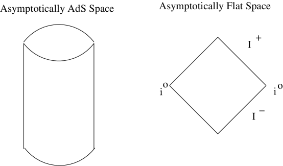
Figure 1: Conformal diagrams of asymptotically AdS space (on the left) and asymptotically flat space (on the right). The two corners marked $i^{0}$ on the asymptotically flat diagram are to be identified.

However, as emphasized in [12], the notion of a conformal boundary is itself not fundamental to AdS/CFT. Rather, this role derives from the convenient way in which the AdS conformal boundary parametrizes the space of possible boundary conditions on propagating fields. Each possible boundary condition defines a bulk theory, which is then dual to a particular non-gravitating field theory (with a particular Lagrangian) on $S^{n-1}\times{\mathbb{R}}$. In contrast, in the asymptotically flat setting, data on the conformal boundary (${\cal I}$) naturally encodes (part of) the information about the state; changing a solution on ${\cal I}^{-}$ (${\cal I}^{+}$) alters the initial (final) data but does not change the dynamics. Instead, boundary conditions are naturally imposed at spacelike infinity, $i^{0}$. This fact will be reviewed in detail in section 2 below.

Although $i^{0}$ is represented by a single point in the conformal compactification, it may be better thought of as a timelike hyperboloid. A particularly nice construction of this ‘boundary’ was given in [13]. The essential point is that physical fields do not admit smooth limits at the point $i^{0}$ of the conformal diagram. Instead, they admit limits which depend (smoothly) on the spacelike direction along which one approaches $i^{0}$ (see e.g. [14, 15]). Thus, for a $d$-dimensional asymptotically flat spacetime, the asymptotics (and, as we will see, the boundary conditions) are associated with functions on the $(d-1)$-dimensional hyperboloid ${\cal H}$ of spacelike directions. Note that ${\cal H}$ is naturally regarded as a signature $(d-2)+1$ manifold, and that it is isometric to the unit $(d-1)$-dimensional de Sitter space. One imagines that ${\cal H}$ may provide a more hospitable home for a dual theory than ${\cal I}$.

The above reasoning is strengthened by a comparison with linear dilaton backgrounds. Despite certain complicating features, string theory in appropriate linear dilaton backgrounds is known to be dual to a (in this case, non-local) non-gravitating theory [6]. The prime example is the case of little string theory [16], where string theory with asymptotics given by the near-horizon limit of $N$ NS5-branes is dual to the low-energy limit of the open string theory on the branes. Here the ground state of the bulk theory is described by the string-frame metric

$$ds^{2}_{string}=dx_{6}^{2}+dz^{2}+d\Omega_{3}^{2},$$ (1)

where $dx^{2}_{6}$ is the 5+1 Minkowski metric, and $d\Omega_{3}^{2}$ is the metric on the unit-sphere. Due to the $dx_{6}^{2}+dz^{2}$ factor, it is clear that the smoothest part of the conformal boundary is just ${\cal I}^{6}$, the null boundary of 6+1 Minkowski space. However, the non-gravitating dual lives on the 5+1 Minkowski space ${\mathbb{R}}^{5,1}$ associated with the branes, and not on ${\cal I}^{6}$. The ${\mathbb{R}}^{5,1}$ is a Lorentz signature spacetime which, as described in [6], can be associated with the large $z$ asymptotics of the linear dilaton spacetime. Roughly speaking, the dual little string theory “lives” at spacelike infinity. This is exactly what we propose in the asymptotically flat context.

Some of the above reasoning was used in [17, 18] to motivate the introduction of a (classical) boundary stress tensor on ${\cal H}$. The stress tensor is a one-point function, and our interest here will be in generalizing the discussion to both the quantum case and to higher ($n$-point) boundary correlators. We begin by reviewing the structure of fields near spatial infinity and discussing possible (infinitesimal) deformations of the usual boundary conditions in section 2. Section 3 then considers variations of the path integral with respect to these boundary conditions. First variations lead to a natural definition of boundary operators. However, subtleties arise for higher correlators.

Section 4 computes boundary two-point functions for operators dual to both massive and massless bulk fields. Two different computations are considered. The first uses the on-shell action and attempts to apply the method used by Gubser, Klenanov, and Polyakov in the AdS context [19]. This method, however, does not appear to give a useful answer to our problem. Instead, non-local analogues of ‘contact terms’ make the result ambiguous. This same feature previdents a straightforward application of the method of [12]. However, our second computation is more successful. Here we first calculate the boundary Wightman function, which is free of contact divergences and well-defined. The result then determines the time-ordered two-point function and guarrantees that it has the expected analytic structure. For comparison, we show that similar results hold for linear dilaton backgrounds dual to little string theory. We close with some further discussion in section 5.

2 Fields near spatial infinity

The complete definition of a field theory generically requires a choice of boundary conditions. In finite volume or in asymptotically anti-de Sitter spacetimes, the fact that signals can propagate from the boundary to the bulk makes the need for boundary conditions especially clear. Boundary conditions are required to fully specify the evolution, as well as to conserve symplectic flux (and thus to make any covariant phase space well-defined).

Boundary conditions in asymptotically flat space are more subtle, but their necessity can be clearly seen in the context of, e.g., non-gravitating scalar field theories on Minkowski space. The scalar wave equation admits many solutions which diverge at spatial infinity, and which cannot be allowed as propagating degrees of freedom if either the energy or the symplectic structure is to be finite. In order to construct a well-defined phase space, one must fix the part of the field associated with such (non-normalizable) modes, allowing only the normalizable part to be dynamical.

The fixed non-normalizable modes are a background structure which play the same roles as do boundary conditions in finite volume. In general, it is necessary only to fix the asymptotic behavior of the field. As a result, we may think of their specification as corresponding to a choice of “boundary conditions at spatial infinity,” and we will use this terminology below. Much the same association between boundary conditions and non-normalizable modes is familiar in the anti-de Sitter context (see e.g. [12, 19, 20, 21]).

Many readers may think of spatial infinity as a single point ($i^{0}$) in the Penrose compactification (see e.g. [22]) of Minkowski space. However, for the reasons stated in section 1, it is better to consider spacelike infinity to be the hyperboloid ${\cal H}$ (see [13, 14, 15]) of spacelike directions. To understand this description, recall that the line element of $d$-dimensional Minkowski space may be written in hyperbolic coordinates as

$$ds^{2}=d\rho^{2}+\rho^{2}\omega_{ij}d\eta^{i}d\eta^{j},$$ (2)

where $\rho^{2}=x_{a}x^{a}$, $\omega_{ij}$ is the metric on the unit $(d-1)$-dimensional Lorentz-signature hyperboloid ${\cal H}$, and $\eta^{i}$ are coordinates on ${\cal H}$. Spacelike infinity is essentially the large $\rho$ limit of the constant $\rho$ hyperboloids.

2.1 Massive Free Scalars

Let us recall the structure of solutions to the (massive) free scalar wave equation on Minkowski space in the hyperbolic coordinates (2). The wave equation is

$$0=(\Box-m^{2})\phi=\left(\frac{1}{\rho^{d-1}}\partial_{\rho}\rho^{d-1}\partial_{\rho}+\frac{1}{\rho^{2}}\nabla^{2}_{\cal H}-m^{2}\right)\phi,$$ (3)

where $\nabla^{2}_{\cal H}$ is the scalar D’Alembertian on ${\cal H}$ and $m^{2}>0$. Any solution to (3) is a linear combination of the modes

$$\Phi_{q,\vec{j}} = \rho^{\frac{2-d}{2}}\hat{I}_{\nu}(m\rho)Y_{q,\vec{j}},\ \ \ {\rm and}$$ (4)

$$\tilde{\phi}_{q,\vec{j}} = \rho^{\frac{2-d}{2}}K_{\nu}(m\rho)Y_{q,\vec{j}},$$ (5)

where $I_{\nu}(m\rho),K_{\nu}(m\rho)$ are the usual modified Bessel functions with $\nu=\sqrt{-q^{2}+\left(\frac{d-2}{2}\right)^{2}}$ and $\hat{I}_{\nu}$ denotes the real part of $I_{\nu}$. Thus, $\hat{I}_{\nu}=\hat{I}_{-\nu}$ for imaginary $\nu$. The $Y_{q,\vec{j}}$ are harmonics on ${\cal H}$ satisfying

$$\nabla_{\cal H}^{2}Y_{q,\vec{j}}=q^{2}Y_{q,\vec{j}}.$$ (6)

At least for normalizable modes, we choose $Y_{q,\vec{j}}$ so that $K_{\nu}(m\rho)Y_{q,\vec{j}}$ is purely positive (negative) frequency in the usual sense on Minkowski space, according to the positive (negative) sign of $q$. Such a choice must be possible since any normalizeable mode has a unique decomposition into positive and negative frequency parts, and the decomposition respects Lorentz invariance. Thus, the ‘projection’ onto the positive frequency subspace commutes with each element of the Lorentz group and is proportional to the identity in any irreducible representation.

The index $\vec{j}$ is an additional label to account for all further degeneracies. For later use, we note that $\vec{j}$ specifes a harmonic $Y_{\vec{j}}$ on $S^{d-2}$. Thus, $\vec{j}$ specifes an integer spin representation of $SO(d-1)$, as well as a state within this representation; e.g, $\vec{j}=(j,m)$ for $SO(3)$. We denote the usual quadratic Casimir of $SO(d-1)$ by $|\vec{j}|^{2}=j(j+d-3)$ for $j\in\mathbb{Z}$.

Let us ask which solutions above represent propagating degrees of freedom. First, propagating modes should be (Klein-Gordon) normalizable at large $\rho$, restricting them to linear combinations of the $\tilde{\phi}_{q,\vec{j}}$. Second, they should be normalizable at small $\rho$. However, for real $\nu$ the Bessel function $K_{\nu}$ grows like $\rho^{-\nu}$ as $\rho\rightarrow 0$. Thus, normalizeable modes satisfy

$$q^{2}\geq\left(\frac{d-2}{2}\right)^{2}.$$ (7)

As noted in, e.g. [23, 24], such $Y_{q,\vec{j}}$ lie in the princpal series of $SO(d-1,1)$ representations, except for the marginal case $q=\pm\frac{(d-2)}{2}$ (which is a member of the complimentary series, see e.g. [25]). As a result, they are delta-function normalizable in $L^{2}({\cal H})$. We take them to satisfy

$$\int_{\cal H}\sqrt{-\omega}\ Y^{*}_{q,\vec{j}}Y_{q^{\prime},\vec{j}^{\prime}}=\delta(q-q^{\prime})\delta_{\vec{j},\vec{j}^{\prime}}.$$ (8)

The $L^{2}({\cal H})$ normalizability of $Y_{q,\vec{j}}$ corresponds to the expected behavior of propagating fields in the distant future and past along the hyperboloid ${\cal H}$ as follows: In the distant past and future, each constant $\rho$ hyperboloid ${\cal H}_{\rho}$ approaches the null cone through the origin. Now, solutions to (3) decay along this null cone in the same manner as the massive Green’s function (as $r^{-(d-1)/2}$). However, the volume of spherical slices of ${\cal H}$ grows only as $r^{d-2}$. Since $r$ increases exponentially with proper time along ${\cal H}$, we see that smooth solutons should lie in each $L^{2}({\cal H}_{\rho})$. In general, normalizable solutions can be obtained through (continuous) superpositions of modes normalized as in (8).

Thus, the modes $\tilde{\phi}_{q,\vec{j}}$ (satisfying (7)) form a basis for the propagating solutions. Other modes which have divergent Klein-Gordon norm at large $\rho$ are non-dynamical and must describe a fixed background. Such modes are specified as part of the “boundary condition” which defines the system. We see that any $\Phi_{q,\vec{j}}$ provides a well-defined boundary condition of this sort. However, such boundary conditions will be of less interest if they are orthogonal to all normalizable modes with respect to the inner product on $L^{2}({\cal H})$. Since the $Y_{q,\vec{j}}$ are eigenstates in $L^{2}({\cal H})$ of the self-adjoint operator $\nabla^{2}_{\cal H}$ with eigenvalue $q^{2}$, and since eigenstates with different eigenvalues are orthogonal, the most interesting boundary conditions will also satisfy (7). As a result, we will often restrict consideration below to those $\Phi_{q,\vec{j}}$ which satisfy (7).

Let us write a general solution as $\phi=\Phi+\tilde{\phi}$, where $\Phi$ is a superposition only of the $\Phi_{q,\vec{j}}$ modes and $\tilde{\phi}$ is a superposition only of the modes $\tilde{\phi}_{q,\vec{j}}$, both satisfying (7). Asymptotically we have

$$I_{\nu}(m\rho)\sim\frac{e^{m\rho}}{\sqrt{2\pi m\rho}},$$ (9)

$$K_{\nu}(m\rho)\sim\frac{e^{-m\rho}}{\sqrt{2m\rho/\pi}},$$ (10)

so that $\Phi,\tilde{\phi}$ can be characterized by arbitrary functions $\alpha,\beta$ on ${\cal H}$ defined by

$$\alpha(\eta) := 2m\lim_{\rho\rightarrow\infty}\rho^{\frac{d}{2}}K_{\nu}(m\rho)\Phi(x)=\lim_{\rho\rightarrow\infty}(\rho^{\frac{d}{2}}K_{\nu}(m\rho))\overleftrightarrow{\partial}_{\rho}\Phi,$$ (11)

$$\beta(\eta) := -2m\lim_{\rho\rightarrow\infty}\rho^{\frac{d}{2}}I_{\nu}(m\rho)\tilde{\phi}(x)=\lim_{\rho\rightarrow\infty}(\rho^{\frac{d}{2}}I_{\nu}(m\rho))\overleftrightarrow{\partial}_{\rho}\tilde{\phi}.$$ (12)

From (9) we see that (11) is independent of the choice of $\nu$. Boundary conditions which require the full solution $\phi=\Phi+\tilde{\phi}$ to be normalizable will be called “fast fall-off” boundary conditions; these clearly impose $\alpha=0$.

Equation (11) describes a natural pairing between boundary conditions and propagating solutions. It is useful to write this pairing in terms of the “boundary product” ($\circ$) of two solutions $\phi_{1}=\Phi_{1}+\tilde{\phi}_{1},\phi_{2}=\Phi_{2}+\tilde{\phi}_{2}$:

$$\phi_{1}\circ\phi_{2}=\int_{\partial{\cal M}}\sqrt{-h}\ \phi_{1}n^{a}\overleftrightarrow{\partial}_{a}\phi_{2}=\int_{\cal H}\sqrt{-\omega}(\alpha_{1}\beta_{2}-\alpha_{2}\beta_{1}),$$ (13)

where $\alpha_{i},\beta_{i}$ are defined as in (11) using $\Phi_{i},\tilde{\phi}_{i}$ respectively. The symbol $\int_{\partial{\cal M}}$ denotes the $\rho\rightarrow\infty$ limit of a family of integrals, each performed over a hyperboloid ${\cal H}_{\rho}$ at fixed $\rho$ having unit outward-pointing normal $n^{a}$ and induced metric $h_{ij}=\rho^{2}\omega_{ij}$. As argued above, one expects propagating modes to have $\beta\in L^{2}({\cal H})$. Clearly, it is also natural to take $\alpha\in L^{2}({\cal H})$, in which case (13) is finite.

2.2 Massless Free Scalars

Let us now consider the special case $m=0$. In this limit the mode functions are no longer exponential at infinity, and their asymptotic behavior now depends on the harmonic on ${\cal H}$. Any solution to the massless Klein-Gordon equation is a linear combination of the modes $\rho^{\lambda_{\pm}}Y_{q,\vec{j}}$, where

$$\lambda_{\pm}=-\frac{d-2}{2}\pm\sqrt{\left(\frac{d-2}{2}\right)^{2}-q^{2}}.$$ (14)

As in the massive case, normalizability considerations require propagating modes to be oscillatory near $\rho=0$, and so again impose (7).

Now, when (7) holds, the massless modes are also oscillatory at large $\rho$. Thus, there is some freedom with regard to which modes are considered to be dynamical and which modes are taken to define boundary conditions. One may check, however, that for the system to have a well-defined phase space (and, in particular, for the symplectic flux through ${\cal H}$ to vanish), that one may allow only a single propagating mode for each $(q,\vec{j})$ satisfying (7). The situation appears to be analogous to that of scalars in AdS with masses close to the Breitenlohner-Freedman bound [26], in which there is a large freedom to choose boundary conditions. We shall assume that some particular choice has been made and denote the corresponding propagating modes by $\tilde{\phi}_{q,\vec{j}}$. We denote another linearly independent set of modes by $\Phi_{q,\vec{j}}$, which we think of as describing particularly simple boundary conditions; namely, those boundary conditions for which the space of propagating modes remains unchanged from the choice made above. We require only that $\Phi_{q,\vec{j}},\tilde{\phi}_{q,\vec{j}}$ are each of the form $f(\rho)Y_{q,\vec{j}}$ and that our modes satisfy the normalization conditions:

$$\Phi^{*}_{q,^{\prime}\vec{j}^{\prime}}\circ\tilde{\phi}_{q,\vec{j}} = -\delta(q-q^{\prime})\delta_{\vec{j},\vec{j}^{\prime}},$$ (15)

$$\langle\tilde{\phi}^{*}_{q,\vec{j}},\tilde{\phi}_{q^{\prime},\vec{j}^{\prime}}\rangle_{KG} := i\int_{\Sigma}\sqrt{g_{\Sigma}}\ \tilde{\phi}^{*}_{q,\vec{j}}n^{a}\overleftrightarrow{\partial}_{a}\tilde{\phi}_{q^{\prime},\vec{j}^{\prime}}={\rm sign}(q)\frac{\mu}{2}|\Gamma(i\mu)|^{2}\delta(q-q^{\prime})\delta_{\vec{j},\vec{j}^{\prime}},$$ (16)

where $\mu=\sqrt{q^{2}-\left(\frac{d-2}{2}\right)^{2}}$ and $\Sigma$ is a Cauchy surface with induced volume element $\sqrt{g_{\Sigma}}$ and unit future-pointing normal $n^{a}$. We have chosen the normalization factor on the right-hand side of (15) in order to mirror the normalization of the massive modes (which is computed in the appendix, see (67)).

For $m^{2}>0$, we parametrized the linear solutions in terms of two functions $\alpha,\beta$ on ${\cal H}$. This is again possible here; for example, one may take

$$\alpha = \sum_{\vec{j}}\int_{q^{2}\geq\left((d-2)/2\right)^{2}}dq\ Y_{q,\vec{j}}\ \tilde{\phi}^{*}_{q,\vec{j}}\circ\Phi\ \ \ {\rm and}$$ (17)

$$\beta = \sum_{\vec{j}}\int_{q^{2}\geq\left((d-2)/2\right)^{2}}dq\ Y_{q,\vec{j}}\ \Phi^{*}_{q,\vec{j}}\circ\tilde{\phi},$$ (18)

where $\circ$ again denotes the boundary product (13). As before, $\tilde{\phi}$ denotes a general linear combination of the $\tilde{\phi}_{q,\vec{j}}$, and $\Phi$ denotes a general linear combination of the $\Phi_{q,\vec{j}}$. Equations (17) are the natural extension to $m^{2}=0$ of $\alpha,\beta$ defined in (11) for $m^{2}>0$. However, for massless fields it is less clear that (17) gives a natural notion of locality on ${\cal H}$. We see that the extraction of $\alpha,\beta$ requires the sort of “mode-dependent renormalization” that is also required in linear dilaton backgrounds (see e.g. [27]).

2.3 Interacting and non-scalar fields

Sections 2.1 and 2.2 above reviewed boundary conditions at $i^{0}$ for linear scalar fields. Parametrizing the space of boundary conditions for an interacting field theory is more difficult. Unless one imposes the “fast fall-off” boundary condition $\alpha=0$, the non-linear interactions become strong near infinity and are hard to control. However, one may linearize the space of boundary conditions about $\alpha=0$. Infinitesimal deformations of the boundary conditions are described by the addition of some linearized solution $\delta\Phi$ (which is again a linear combination of the modes $\Phi_{q,\vec{j}}$ from sections 2.1 or 2.2). In this way, it is meaningful to vary even a non-linear theory with respect to $\alpha$, so long as one evaluates all such variations at $\alpha=0$. A similar structure is commonly used to discuss boundary conditions of massive scalar fields in AdS (see e.g. [28]), and is the best that one can expect for masses sufficiently far above the Breitenloher-Freedman bound, where they correspond to non-renormalizable deformations of the dual field theory.

For the sake of clarity, we have concentrated on scalar field theory. The generalization to fields of higher spin is straightforward. For concreteness, let us briefly discuss the case of the gravitational field itself. Linearized gravitational fluctuations about asymptotically flat space are similar to the linear scalar solutions reviewed above (see e.g. [29, 30, 31]. We may take, e.g., the boundary conditions of [32] (for $d=4$) or [17] (for $d\geq 4$) to define a notion of “fast fall-off.” Only these boundary condtions are asymptotically flat. Other boundary conditions which break asymptotic flatness may then be studied perturbatively, much as was done for the massless scalar field. This will be sufficient to construct the asymptotically flat analogue of the ‘boundary correlators’ used in the AdS/CFT dictionary, which are related to infinitesimal variations of the path integral with respect to the boundary conditions. The issue of finite deformations of asymptotic flatness is more complicated, however. While a reasonable theory of such deformations may exist, it is clear from e.g. [30] in $d=4$ (or [31] in higher dimensions) that such deformations destroy the entire asymptotic structure near spatial infinity. One expects that such deformations correspond to non-renormalizable deformations of the dual theory.

2.4 A Warning about Locality

In the above sections we described boundary conditions at spatial infinity in terms of a function $\alpha$ on ${\cal H}$. This presentation was chosen to maximize similarity with the asymptotically AdS case, where boundary conditions are conveniently represented by functions on the conformal boundary. However, we warn the reader that the corresponding notion of locality on ${\cal H}$ is less useful than on the analogous AdS boundary.

This is not a surprise from the standpoint of gauge/gravity duality. In AdS/CFT, it is well known that the local properties of the CFT are related to the asymptotic structure of AdS space. One sees this already at the level of symmetries: certain (asymptotic) AdS isometries induce a dilation on the conformal boundary, so that taking a bulk operator to the boundary naturally results in a local dual operator. Similarly, the wave equation associates point sources on the boundary with a position-dependent length scale in the bulk which goes to zero at the boundary. Since it was observed in [27, 33] that such properties fail to hold with either linear dilaton or asymptotically flat boundary conditions, we may expect the corresponding locality properties to fail as there well.

Let us take a more precise look at this connection. Since deformations of AdS boundary conditions correspond to the addition of CFT sources, the ‘locality’ of such sources should be reflected in corresponding local properties of the boundary conditions. Indeed, such a locality property was pointed out in [12] in the Euclidean context: Consider a deformation of AdS boundary conditions described by some $\delta\alpha$ of compact support on the boundary. A given bulk solution $\phi$ will be deformed in a complicated way, even at parts of the boundary far from the support of $\delta\alpha$. However, away from the support of $\delta\alpha$, the new solution will still respect the original boundary conditions. One often says that $\delta\phi$ is “normalizable” outside the support of $\delta\alpha$. The same is true in the Lorentzian setting where, as shown in [34, 35], in the Poincaré patch one may choose the deformation to vanish in an open set whose intersection with the boundary contains all points outside the support of $\delta\alpha$.

In contrast, this feature does not hold in our asymptotically flat context. While $\delta\alpha$ controls the leading $\rho$ behavior, it does not provide the same ‘local’ description of other non-normalizable terms in $\Phi$. It is instructive to compute the ‘bulk-boundary propagator’ $G_{\partial}$ for asymptotically flat space: One begins with a bulk Green’s function $G(x,x^{\prime})$ satisfying, say, Feynmann boundary conditions. One then takes $x^{a}=\rho\hat{\eta}^{a}$ for some spacelike unit vector $\hat{\eta}^{a}$ and considers the large $\rho$ limit. To obtain a finite result, one rescales the limit by the same function of $\rho$ as is used to define the boundary value $\beta$ in (11).

One finds

$$G(x,x^{\prime})\sim m^{d-2}\frac{e^{-m|x-x^{\prime}|}}{(m|x-x^{\prime}|)^{\frac{d-1}{2}}}=m^{d-2}\frac{e^{-m\rho}e^{+mx^{\prime}{}^{a}\hat{\eta}_{a}}}{(m\rho)^{\frac{d-1}{2}}}\left(1+{\cal O}(\rho^{-1})\right),$$ (19)

so that

$$G_{\partial}(\hat{\eta},x^{\prime})\sim-\sqrt{\frac{2m}{\pi}}\lim_{\rho\rightarrow\infty}\rho^{\frac{d-1}{2}}e^{m\rho}G(x,x^{\prime})=-m^{\frac{d-2}{2}}\sqrt{\frac{2}{\pi}}e^{mx^{\prime}{}^{a}\hat{\eta}_{a}}.$$ (20)

But now if we consider $x^{\prime}{}^{a}=\rho\hat{\eta}^{\prime}{}^{a}$ as $\rho\rightarrow\infty$, we find that (20) diverges whenever $\hat{\eta}^{\prime}{}^{a}\hat{\eta}_{a}>0$. The non-normalizable behavior is not localized at the point $\hat{\eta}\in{\cal H}$.

How is this feature to be interpreted? We argue in the rest of this work that it is merely another sign of non-locality in the dual theory. In particular, we are able to calculate boundary two-point functions in section 4. We also show in section 4.3 that the above feature also arises for the linear dilaton background dual to little string theory [6], and is therefore not an obstruction to the existence of a meaningful dual.

3 Boundary Operators, Path integrals, and the S-matrix

In anti-de Sitter space, boundary correlators are variations of either the partition function [12] (in Euclidean signature) or of a transition amplitude $\langle\psi_{+}|\psi_{-}\rangle$ [19, 20, 21] (in Lorentz signature, see [36] for details). In the latter case, the variation is performed holding $|\psi_{-}\rangle$ fixed in the far past (retarded boundary conditions) and holding $|\psi_{+}\rangle$ fixed in the far future (advanced boundary conditions). By letting $|\psi_{+}\rangle$ and $|\psi_{-}\rangle$ range over a complete set of states, one defines a full boundary operator. It is such operators which are most naturally dual to CFT operators under the AdS/CFT correspondence. Up to a certain rescaling, they are simply boundary limits of bulk operators (see e.g. [37]).

Our goal here is to investigate the analogous construction in asymptotically flat space. For concreteness we again consider scalar field theory, but the analysis generalizes directly to higher spin fields. A study of first variations will motivate a definition of ‘boundary operators.’ We then address higher variations and find that issues involving contact terms are more complicated than in AdS space. Nevertheless, boundary n-point functions may be defined directly in terms of the above-mentioned boundary operator. We will return to these issues again in section 4.

We begin with a (Lorentz-signature) path integral of the form $\langle\psi_{+}|\psi_{-}\rangle=\int D\phi e^{iS}$, where the integral is only over fields $\phi$ satisfying the fast fall-off boundary conditions of section 2. Note that we have absorbed factors containing the wavefunctions of the states $|\psi_{\pm}\rangle$ into $S$. These factors contribute extra boundary terms to $S$ at the past and future boundaries $\Sigma_{\pm}$. While they are localized on $\Sigma_{\pm}$, the particular form of these boundary terms is generically non-local within $\Sigma_{\pm}$.

To deform our boundary conditions by an infinitesimal amount $\alpha$, we shift the domain of integration by some (infinitesimal) $\Phi$ which satisfies either (11) or (17) for this $\alpha$. We require $\Phi$ to be a solution to the classical equations of motion up to some fast fall-off configuration. That is, there must be some fast fall-off configuration $\tilde{\phi}$ (which need not be a solution) such that $\Phi-\tilde{\phi}$ is a classical solution .

To vary $\langle\psi_{+}|\psi_{-}\rangle$, we must understand how the action $S$ depends on the boundary conditions. This depends on how both the bulk dynamics and the states $|\psi_{\pm}\rangle$ vary with $\Phi$. In AdS, one would choose $\Phi$ to vanish on $\Sigma_{\pm}$ so as to preserve advanced boundary conditions on $|\psi_{+}\rangle$ and retarded boundary conditions on $|\psi_{-}\rangle$. However, as discussed in section 2.4, such a choice is not in general possible in the asymptotically flat context. Thus, we must allow an arbitrary deformation of $S$ on $\Sigma_{\pm}$ and attempt to define our boundary operators so that they are independent of this ambiguity. We will, however, require at each perturbative order in $\Phi$ that i) $S$ yields the same bulk equations of motion as for $\Phi=0$ and that ii) $S$ be stationary on classical solutions.

Such principles do not fully determine the desired extension of $S$, but they do constrain the possibilities. Suppose that the action for $\Phi=0$ takes the standard form

$$S_{0}=-\int_{\cal M}\left(\frac{1}{2}\partial\phi^{2}+V(\phi)\right)\sqrt{-g}+\int_{\Sigma_{+}\cup\Sigma_{-}}S_{\pm}.$$ (21)

Here ${\cal M}$ represents a volume of spacetime to the future of a Cauchy surface $\Sigma_{-}$ on which $\psi_{-}$ is specified, and to the past of an analogous $\Sigma_{+}$ on which $\psi_{+}$ is specified. The boundary terms $S_{\pm}$ on $\Sigma_{\pm}$ depend on the details of the states $\psi_{\pm}$. In terms of $\tilde{\phi}=\phi-\Phi$, we seek an action of the form $S=S_{0}[\phi]+S_{1}[\Phi,\tilde{\phi}]$ where $S_{1}$ is a boundary term linear in $\Phi$ such that variations $\delta S$ performed holding $\Phi$ fixed vanish on solutions (to first order in $\Phi$). One finds

$$\delta S_{0}=\int_{\cal M}\sqrt{-g}\left(\nabla^{2}\phi-V^{\prime}(\phi)\right)\delta\phi-\int_{\partial\cal M}\sqrt{-h}(n^{a}\partial_{a}\phi)\delta\phi+\int_{\Sigma_{+}\cup\Sigma_{-}}B_{\pm}.$$ (22)

Here $\partial{\cal M}$ denotes only the boundary of $\partial{\cal M}$ at spatial infinity; i.e., the part of ${\cal H}$ which lies between the Cauchy surfaces $\Sigma_{\pm}$.

The bulk term in (22) contains just the desired equations of motion. Since $\delta\phi=\delta\tilde{\phi}$ and $\int_{\partial\cal M}\sqrt{-h}(n^{a}\partial_{a}\tilde{\phi})\delta\tilde{\phi}$ vanishes for any normalizable solution $\tilde{\phi}$, on appropriate solutions we find

$$\delta S_{0}=-\int_{\partial\cal M}\sqrt{-h}(n^{a}\partial_{a}\Phi)\delta\tilde{\phi}+\int_{\Sigma_{+}\cup\Sigma_{-}}B_{\pm}.$$ (23)

The term at $\partial{\cal M}$ in (23) does not vanish and will be cancelled by the variation $\delta S_{1}$. One would like to use the condition $B_{\pm}=0$ to impose boundary conditions on solutions at $\Sigma_{\pm}$, but it is not clear whether such conditions are compatible with the equations of motion for $\Phi\neq 0$. To achieve compatibility, the boundary terms at $\Sigma_{\pm}$ may need to be corrected by a term in $S_{1}$. Thus, $S_{1}$ must be of the form

$$S_{1}=\int_{\partial\cal M}\sqrt{-h}(\tilde{\phi}+c)(n^{a}\partial_{a}\Phi)+\int_{\Sigma_{+}\cup\Sigma_{-}}B_{\pm}^{(1)}\Phi+O(\alpha^{2}),$$ (24)

where $c$ is some fixed function on $\partial{\cal M}$ and $B_{\pm}^{(1)}$ are linear operators on $\Sigma_{\pm}$. Below we take $c=0$, but a more general choice merely shifts our boundary operators by some set of $c$-numbers. We will, however, need to define our boundary operators in a way that is independent of $B_{\pm}^{(1)}$.

We are now ready to vary the boundary conditions in our path integral, shifting the region of integration by $\delta\phi=\delta\Phi$. With $S=S_{0}+S_{1}$, this variation yields

$$\delta\langle\psi_{+}|\psi_{-}\rangle\Big{|}_{\Phi=0} = \int D\phi\ ie^{iS}\delta S\Big{|}_{\Phi=0}$$ (25)

$$= \int D\phi\ ie^{iS}\Biggl{[}\int_{\cal M}\sqrt{-g}\left(\nabla^{2}\phi-V^{\prime}(\phi)\right)\delta\Phi+\int_{\partial\cal M}\sqrt{-h}\ \phi n^{a}\overleftrightarrow{\partial_{a}}\delta\Phi$$ (27)

$$\hskip 71.13188pt+\int_{\Sigma_{+}\cup\ \Sigma_{-}}B_{\pm}(\delta\Phi)\Big{|}_{\Phi=0}+\int_{\Sigma_{+}\cup\ \Sigma_{-}}B_{\pm}^{(1)}\delta\Phi\Biggr{]}$$

$$= i\int_{\partial\cal M}\sqrt{-h}\ \langle\psi_{+}|\hat{\phi}|\psi_{-}\rangle n^{a}\overleftrightarrow{\partial_{a}}\delta\Phi+\int_{\Sigma_{+}\cup\Sigma_{-}}B_{\pm}^{(1)}\delta\Phi,$$ (28)

where in the last step we have used the fact that the matrix elements of both $B_{\pm}$ and the equations of motion vanish and we have introduced the local bulk quantum field operator $\hat{\phi}(x)$. We shall reserve the symbol $\phi(x)$ for c-number field configurations, such as classical solutions or configurations over which one integrates in the path integral.

We wish to define a boundary operator which is independent of $B_{\pm}^{(1)}$, as this term is associated with the arbitrary extension of the state $|\psi_{\pm}\rangle$ to non-zero $\Phi$. It is thus natural to define the boundary operator $\hat{\phi}_{\partial}(\alpha)$ to be ($-i$ times) the part of (25) given by a local integral over $\partial{\cal M}$:

$$\hat{\phi}_{\partial}(\alpha):=\int_{\partial{\cal M}}\sqrt{-h}\ \hat{\phi}(x)n^{a}\overleftrightarrow{\frac{\partial}{\partial{x}^{a}}}\left(\Phi[\alpha]\right)(x),$$ (29)

for any function $\alpha$ on ${\cal H}$. Here $\Phi[\alpha]$ is any solution associated with $\alpha(\eta)$ through (11) or (17). This is a direct analogue of the familiar structure from AdS space, and in particular parallels the construction of AdS asymptotic creation and annihilation operators in [38]. For $m^{2}>0$, the discussion at the end of section 2.1 implies that (29) is well-defined when acting on a dense set of states.

We may also consider the higher correlators

$$\langle\psi_{+}|\hat{\phi}_{\partial}(\alpha_{1})\hat{\phi}_{\partial}(\alpha_{2})\dots\hat{\phi}_{\partial}(\alpha_{k})|\psi_{-}\rangle.$$ (30)

These Wightman functions are defined directly by repeated application of the boundary operators (29) to the state $|\psi_{-}\rangle$, though through (29) we see that they satisfy

$$\langle\psi_{+}|\hat{\phi}_{\partial}(\alpha_{1})\hat{\phi}_{\partial}(\alpha_{2})\dots\hat{\phi}_{\partial}(\alpha_{k})|\psi_{-}\rangle=\int_{\partial{\cal M}}\sqrt{-h}d^{d-1}\eta_{1}\ \dots\ \int_{\partial{\cal M}}\sqrt{-h}d^{d-1}\eta_{k}$$ (31)

$$\times \Phi[\alpha_{1}](x_{1})\dots\Phi[\alpha_{k}](x_{k})n_{1}^{a}\overleftrightarrow{\frac{\partial}{\partial{x_{1}}^{a}}}\dots n_{k}^{a}\overleftrightarrow{\frac{\partial}{\partial{x_{k}}^{a}}}\langle\psi_{+}|\hat{\phi}(x_{1})\ \dots\ \hat{\phi}(x_{k})|\psi_{-}\rangle.\ \ \ \ \ \$$ (32)

Here the $(\rho_{i},\eta_{i})$ are the hyperbolic coordinates of $x_{i}$.

It is also interesting to discuss time-ordered boundary correlators defined by

$$\langle\psi_{+}|T\left(\hat{\phi}_{\partial}(\alpha_{1})\ \dots\ \hat{\phi}_{\partial}(\alpha_{n})\right)|\psi_{-}\rangle:=\int_{\partial{\cal M}}\sqrt{-h}d^{d-1}\eta_{1}\ \dots\ \int_{\partial{\cal M}}\sqrt{-h}d^{d-1}\eta_{k}$$ (33)

$$\times \Phi[\alpha_{1}](x_{1})\dots\Phi[\alpha_{k}](x_{k})n_{1}^{a}\overleftrightarrow{\frac{\partial}{\partial{x_{1}}^{a}}}\dots n_{k}^{a}\overleftrightarrow{\frac{\partial}{\partial{x_{k}}^{a}}}\langle\psi_{+}|T\left(\hat{\phi}(x_{1})\ \dots\ \hat{\phi}(x_{k})\right)|\psi_{-}\rangle.\ \ \ \ \ \$$ (34)

In the AdS context, time-ordered $k$-point boundary correlators are $k$th functional derivatives of the transition amplitude $\langle\psi_{+}|\psi_{-}\rangle$. However, due to contact terms, this relation holds only when the supports of the variations do not overlap. With AdS asymptotics, it is not difficult to choose the $\Phi[\alpha_{i}]$ to have non-overlapping support in the bulk spacetime. However, this is not in general possible in asymptotically flat space. As noted in section 2.4, even for functions $\alpha_{1},\alpha_{2}$ with well separated supports on ${\cal H}$, the supports of the bulk functions $\Phi[\alpha_{1}],\Phi[\alpha_{2}]$ must overlap. Thus, for $k>1$, time-ordered $k$-point functions are variations of the path integral only up to i) terms at $\Sigma_{\pm}$ as in the discussion of one-point functions and ii) additional (typically divergent) terms associated with contact terms in the bulk. We refer to terms of type (ii) as “contact terms” even though they occur for boundary operators with disjoint supports.

4 Boundary Correlators

Having discussed the general structure of our boundary operators, we now compute boundary two-point functions. We attempt two computations, though only one succeeds. The first (section 4.1) is an attempt to follow the analogue of the procedure [19] used by Gubser, Klebanov, and Polyakov for AdS/CFT. Unfortunately, this approach suffers from the divergent non-local contact terms mentioned in section 3 above. As a result, it is unclear which non-local terms one should substract to obtain the correct (finite) two-point function. The same non-local contact terms prevent a straightforward application of the method of [12].

On the other hand, we show (section 4.2) that the boundary Wightman two-point functions are readily calculated using the basic definition (29). The result is finite and unambiguous, and it leads to a (well-defined) time-ordered boundary two-point function with the expected analytic structure. To gain additional perspective on the above issues, we consider the same calculations in linear dilaton backgrounds in section 4.3 and find similar results.

4.1 Boundary 2-point functions via variations of the action

We noted in section 3 that our time-ordered boundary two-point functions are the second variations of a bulk partition function, up to contact terms and terms at $\Sigma_{\pm}$. In the limit in which the bulk system is semi-classical, this variation is just the on-shell variation of the bulk action:

$$\frac{\langle|T\left(\hat{\phi}_{\partial}(\delta_{1}\alpha)\ \hat{\phi}_{\partial}(\delta_{2}\alpha)\right)|0\rangle}{\langle 0|0\rangle}\approx-\delta_{1}\delta_{2}S+\ {\rm contact\ terms}\ +\ {\rm terms\ at}\ \Sigma_{\pm}.$$ (35)

To compute such correlators, we study variations of the semi-classical action and attempt to remove the extraneous terms. This is essentially the approach to calculating boundary correlators (in AdS) advocated in [19]. Since the goal is to obtain time-ordered vacuum correlators, one expects that one may avoid consideration of future and past boundary terms by analytic continuation to Euclidean signature and taking $\Sigma_{\pm}$ to infinity. We shall do so below.

The variation $\delta_{1}\delta_{2}S$ evaluated at $\phi=0$ depends only on the part of the action quadratic in $\phi$; it is independent of any couplings of $\phi$ to itself or to any other fields (including gravity). The calculation is similar to (22) and yields:

$$\delta_{1}\delta_{2}S=-\int_{\partial\cal M}\sqrt{-h}\ \delta_{1}\Phi[\alpha]\ n^{a}\partial_{a}\delta_{2}\Phi[\alpha],$$ (36)

where $\delta_{1}\alpha$, $\delta_{2}\alpha$ are now functions on $S^{d-1}$ and $\delta_{1}\Phi[\alpha],\delta_{2}\Phi[\alpha]$ are solutions (up to normalizable terms) associated with $\delta_{1}\alpha$, $\delta_{2}\alpha$ through the Euclidean version of (11) or (17).

As usual, the calculation is most straightforward using normal modes. Thus we take

$$\delta_{1}\alpha=\epsilon_{1}Y_{\vec{\ell}_{1}},\ \ \ \delta_{2}\alpha=\epsilon_{2}Y_{\vec{\ell}_{2}},$$ (37)

where $Y_{\vec{\ell}_{2}}$ are harmonics on $S^{d-1}$ and $\epsilon_{1},\epsilon_{2}$ are (infinitesimal) constants. The notation here matches our previous notation for harmonics on the sphere; e.g. $|\vec{\ell}|^{2}=\ell(\ell+d-2)$. For a massive field $\phi$ we have

$$\delta_{1}\Phi[\alpha]=\epsilon_{1}\rho^{\frac{2-d}{2}}I_{\nu_{1}}(m\rho)Y_{\vec{\ell}_{1}},$$ (38)

$$\delta_{2}\Phi[\alpha]=\epsilon_{2}\rho^{\frac{2-d}{2}}I_{\nu_{2}}(m\rho)Y_{\vec{\ell}_{2}},$$ (39)

where $\nu=\ell+\frac{d-2}{2}$.

To evaluate (36), we make use of the asymptotic expansion:

$$I_{\nu}(z)=\frac{1}{\sqrt{2\pi z}}A_{\nu}(z)+\frac{\cos\left((\nu+\frac{1}{2})\pi\right)}{\sqrt{2\pi z}}B_{\nu}(z),$$ (40)

where

$$A_{\nu}(z) := e^{z}\sum_{k=0}^{\infty}\frac{(-1)^{k}}{(2z)^{k}}\frac{\Gamma(\nu+k+\frac{1}{2})}{k!\Gamma(\nu-k+\frac{1}{2})},\ \ \ {\rm and}$$ (41)

$$B_{\nu}(z) := e^{-z}\sum_{k=0}^{\infty}\frac{1}{(2z)^{k}}\frac{\Gamma(\nu+k+\frac{1}{2})}{k!\Gamma(\nu-k+\frac{1}{2})}.$$ (42)

We have obtained (40,41) from [39], though in [39], the coefficient of $B_{\nu}$ in (40) involves $\exp(\pm(\nu+\frac{1}{2})\pi i)$ instead of the cosine. This ambiguity is described as a “Stokes Phenomenon.” Since we require a real solution, we have simply taken the average of the two expansions. However, the result below is identical if one uses $\exp(\pm(\nu+\frac{1}{2})\pi i)$ and chooses the sign in a way which depends only on $\nu$.

Inserting expressions (40,41) into (36) yields three kinds of terms:

1. Terms involving $B_{\mu_{1}}\partial_{\rho}B_{\mu_{2}}$, which are too small to contribute as $\rho\rightarrow\infty$.

2. Terms involving $A_{\mu_{1}}\partial_{\rho}B_{\mu_{2}}$ and $B_{\mu_{1}}\partial_{\rho}A_{\mu_{2}}$. These give finite contributions, which cancel against each other.

3. Divergent terms involving the expressions $A_{\mu_{1}}\partial_{\rho}A_{\mu_{2}}$.

Recall that the form of the action has only been fixed up to ${\cal O}(\alpha^{2})$ terms. It is natural to choose such terms to precisely cancel the terms of type (iii), which arise only from non-normalizable terms in the expansion of (40). As we will discuss in section 4.3 below, this appears to be the analogue of the procedure followed in [40] for massless fields in a linear dilaton background. One may hope that this is equivalent to subtracting the extra “contact terms” noted above, together with any other contact divergences inherent in the correlator itself. After making this choice, we find

$$\langle 0|T\left(\hat{\phi}_{\partial}(Y_{\vec{\ell}_{1}})\hat{\phi}_{\partial}(Y_{\vec{\ell}_{2}})\right)|0\rangle=0$$ (43)

for all $m^{2}>0$.

We may also compute the correlator for $m=0$. In this case, the radial mode functions are simply $\rho^{\lambda}$ for appropriate $\lambda$; there is no apparent mixing between normalizable modes $(\tilde{\phi})$ and non-normalizable modes $(\Phi)$. Thus, subtracting the $m=0$ analogue of the type (iii) terms again yields (43).

The fact that (43) vanishes identically suggests caution in interpreting the result. Indeed, as remarked above, the particular subtractions we have used are far from well-justified. Recall that for $m^{2}>0$ our subtractions are non-analytic in $q^{2}$, and thus do not qulitatively differ from the sort of finite remainder terms that one would expect. On general grounds one might also expect to require a non-analytic subtraction for $m^{2}=0$ (though we did not use one there). Thus, this approach to calculating the 2-point function appears to be inherently ambiguous.

We note that the method of [12] will meet with similar problems: In AdS/CFT it avoids divergences by working with separated operators, but our asymptotically flat computations generate non-local “contact terms” which can diverge even at separated points. Thus, we must seek another approach.

4.2 Boundary correlators via the Wightman Function

One might like to calculate 2-point functions directly from the basic definition of the boundary operator (29). This is indeed possible if one focusses on Wightman functions, and such an approach turns out to have several advantages. For example, in any local field theory, the Wightman function is a well-defined bi-distribution, meaning that it is finite when integrated against two smooth functions which behave appropriately at infinity. There are thus no divergences from contact terms. The same is true of Wightman boundary correlators in AdS, and we will see that the same is again true for asymptotically flat boundary two-point functions.

The computation is straightforward using the representation of the bulk Wightman function $W(x,x^{\prime})$ as a sum over Klein-Gordon-normalized positive frequency modes. Since modes with $q>0$ are positive frequency while modes with $q<0$ are negative frequency, and since propagating modes satisfy (7), for any $m\geq 0$ we have

$$W(x,x^{\prime})=\int_{q>\frac{d-2}{2}}dq\sum_{\vec{j}}\frac{2}{\mu|\Gamma(i\mu)|^{2}}\phi^{*}_{q,\vec{j}}(x)\phi_{q,\vec{j}}(x^{\prime}).$$ (44)

Here we have used expression (67) or (15) for the Klein-Gordon norms of our modes.

Taking the boundary product of $W$ with two modes $\Phi_{q_{1},\vec{j}_{1}},\Phi^{*}_{q_{2},\vec{j}_{2}}$ with $q\geq\frac{d-2}{2}$ and using the orthonormality of the $Y_{q,\vec{j}}$ we find

$$W_{\partial}(q_{1},\vec{j}_{1},q_{2},\vec{j}_{2}) := \langle 0|\hat{\phi}_{\partial}(Y_{q_{1},\vec{j}_{1}})\hat{\phi}_{\partial}(Y^{*}_{q_{2},\vec{j}_{1}})|0\rangle$$ (45)

$$= \frac{2}{\mu|\Gamma(i\mu)|^{2}}\delta(q_{1}-q_{2})\delta_{\vec{j}_{1},\vec{j}_{2}}\ \ \ {\rm for}\ \ q_{1},q_{2}\geq\frac{q-2}{2}.$$ (46)

The boundary Wightman function vanishes for other modes. The result is finite, non-zero, independent of $m$, and insensitive to the Bessel Stokes phenomenon.

From the result (45), one may now unambiguously compute the associated time-ordered 2-point function. To do so, one need only write (45) as

$$W_{\partial}(q_{1},\vec{j}_{1},q_{2},\vec{j}_{2}):=\int_{0}^{\infty}\frac{d\mu}{\pi|\Gamma(i\mu)|^{2}}W^{\cal H}_{q(\mu)}(q_{1},\vec{j}_{1},q_{2},\vec{j}_{2}),$$ (47)

where $q(\mu)=\sqrt{\mu^{2}+\left(\frac{d-2}{2}\right)^{2}}$ and

$$W^{\cal H}_{q}(q_{1},\vec{j}_{1},q_{2},\vec{j}_{2})=\frac{\pi}{q}\delta(q-q_{1})\delta(q-q_{2})\delta_{\vec{j}_{1},\vec{j}_{2}}$$ (48)

is the Wightman function on ${\cal H}$ for a free scalar field of mass $q$. The is essentially the Källen-Lehman representation of the Wightman function on ${\cal H}$. The time-ordered two-point function is then

$$\langle 0|T\left(\hat{\phi}_{\partial}(Y_{\vec{\ell}_{1}})\hat{\phi}_{\partial}(Y_{\vec{\ell}_{2}})\right)|0\rangle=\int_{0}^{\infty}\frac{d\mu}{\pi|\Gamma(i\mu)|^{2}}G^{F,{\cal H}}_{q(\mu)}(q_{1},\vec{j}_{1},q_{2},\vec{j}_{2}),$$ (49)

where $G^{F,{\cal H}}_{q(\mu)}$ is the Feynmann Green’s function on ${\cal H}$ for a free scalar field of mass $q$.

Note that there is a branch cut beginning at $q=\frac{d-2}{2}$ associated with the continuum of propagating bulk states. Indeed, one sees that the analytic structure is determined by the Källen-Lehman spectral function of the boundary operator $\phi_{\partial}$, which is in turn determined directly by the spectrum of bulk states.

4.3 Little String Theory

Despite our success with methods based on Wightman functions, we have seen that computations of asymptotically flat boundary 2-point functions by analogy with either [19] or [12] faced serious difficulties. Now, as mentioned in the introduction, linear dilaton backgrounds dual to little string theory share many features of asymptotically flat spacetimes. As a result, one may hope to gain further insight by pursuing this analogy in detail. To that end, we now consider boundary two-point functions associated with a scalar field in the linear dilaton background dual to little string theory (namely, in the near-horizon solution for $N$ coincident $NS5$-branes [6]). We will see that, despite the evident success of the Gubser-Klebanov-Polyakov method in this context [40, 41], the same issues identified in section 4.1 also arise in linear dilaton backgrounds.

Let us first briefly review the linear dilaton spacetimes of interest. In the string frame, the near horizon description of $N$ coincident $NS5$-branes takes the familiar form

$$ds^{2}_{string}=dx_{6}^{2}+dz^{2}+\frac{N}{m_{s}^{2}}d\Omega_{3}^{2},$$ (50)

$$g=g_{0}e^{-\frac{zm_{s}}{\sqrt{N}}},$$ (51)

where $dx_{6}^{2}$ is the 6-dimensional Euclidean metric and $m_{s}$ is the string mass scale. In the strong coupling regime at large negative $z$, the physics is more properly described by the near-horizon metric of $N$ $M5$-branes on an $S^{1}$. However, we will be interested only in the asymptotics at large $z$ where the corrections are heavily suppressed.

It is natural to consider a scalar field minimally coupled to the Einstein frame metric. This metric takes the tantalizing form

$$ds^{2}=\rho^{2}(dy_{6}^{2}+\frac{1}{16}d\Omega^{2}_{3})+d\rho^{2},$$ (52)

where $\rho=\frac{4\sqrt{N}}{m_{s}}e^{zm_{s}/4\sqrt{N}}$ and $dy_{6}^{2}$ is again the 6-dimensional Euclidean metric, but with rescaled coordinates $y_{i}=\frac{m_{s}}{4\sqrt{N}}x_{i}$. While (52) is not asymptotically flat, the metric components involve the same powers of $\rho$ as in flat Minkowski space.

Massless scalar fields minimally coupled to (52) were studied in [40]. We now consider massive minimally coupled fields. Solutions to the massive scalar wave equation are given by

$$\Phi_{k,\vec{j}} = \frac{1}{(2\pi)^{3}}Y_{\vec{j}}e^{ik_{a}y^{a}}I_{\nu}(m\rho),$$ (53)

$$\Phi_{k,\vec{j}} = \frac{1}{(2\pi)^{3}}Y_{\vec{j}}e^{ik_{a}y^{a}}K_{\nu}(m\rho),$$ (54)

with $\nu=\sqrt{k^{2}+16j(j+2)+16}$ and $\vec{j}$ labeling a complete set of states in $SO(4)$. Since the string coupling goes to zero at large $\rho$, M-theoretic corrections to (52) die off faster than $e^{-\lambda\rho}$ for any $\lambda$ and the corrections to these mode functions will be correspondingly small, though they might result in some “mixing” through the addition of a further normalizeable piece $CK_{\nu}(m\rho)$ to the “non-normalizable” mode $I_{\nu}(m\rho)$ associated with some particular boundary conditions. Note, however, that $C$ must be determined by $k^{2}$ and $j$ ($C=C(k^{2},j)$) and that $C$ is real (at least in Euclidean signature).

Let us now consider the 2nd on-shell variation of the classical action. As in section 4.1, three kinds of terms will be generated. The finite (type ii) terms again cancel for any $C(k^{2},j)$, so long as the Stokes phenomenon is again dealt with as in section (4.1). Terms containing $A_{\nu_{1}}\partial_{\rho}A_{\nu_{2}}$ are divergent. As in the asymptotically flat case, subtracting such terms yields a time-ordered two-point function which vanishes for any $m^{2}>0$.

However, for the same reasons as in section 4.1, the divergences associated with $A_{\nu_{1}}\partial_{\rho}A_{\nu_{2}}$ terms are again non-analytic in $k$; they do not have the form of familiar contact terms. To interpret these divergences, recall that little string theory is non-local [16]. We might therefore expect that any time-ordering operation is more complicated than for a local theory, and may lead to divergences even at separated points. In fact, the same argument as in section 3 suggests that the variation of the path integral will differ from the time-ordered two-point function by non-local contact terms. The key point is that the linear dilaton background’s bulk-boundary Green’s function is non-local in precisely the sense described in section 2.4 for asymptotically flat space. To see this, consider the non-normalizable solution

$$\Phi=\frac{1}{(2\pi)^{6}}\int dk\ \Phi_{k,\vec{\ell}}.$$ (55)

The leading behavior is $\Phi\sim\delta(x)Y_{\vec{\ell}}\ \frac{e^{-m\rho}}{\sqrt{2}\pi m\rho}$, but the non-analytic dependence of $A_{\nu}$ on $k$ means that $\Phi$ contains subleading non-normalizable terms not localized at $x=0$. While this observation again encourages the subtraction of such divergences, it raises the disturbing prospect that the remaining finite part may be contaminated with unwanted (but finite) non-local “contact” terms.

Let us also briefly compare the computations for massless fields. The linear dilaton calculation was performed in [40], and the asymptotically flat case was discussed in section 4.1 above. Both calculations obtain a finite answer by subtracting only divergences analytic in $k$. However, both manifest signs of non-locality via the need for ‘mode-dependent renormalization’ [27, 42, 40]. One apparent difference is that the asymptotically flat result vanished identically. However, despite the removal only of divergences analytic in $k$, there is no local bulk-boundary propagator and it is possible that the finite remainders are again contaminated by non-local contact terms, and any comparison of the results should proceed with caution.

We see that there is a strong similarity between the issues that arise in the asymptotically flat and linear dilaton contexts. Of course, there is also a significant difference. Namely, as shown in [40, 41], at least for massless scalar fields, one does appear to obtain a physically interesting time-ordered two-point function by applying the analogue of the Gubser-Klebanov-Polyakov method [19] along with a naive subtraction of leading divergences. In particular, [40] showed that at small momenta such computations precisely agree the results of the theory on M5-branes. Furthermore, in the thermally excited context, [41] found such computations to precisely agree with those of [43] performed in little string theory. Finally, [44] argued that the analytic structure of the two-point function so-obtained properly matches expectations from the bulk spectrum of states. The evident success of such comparisons suggests that a unique prescription for subtracting non-local contact terms can be established for linear dilaton backgrounds and thus, perhaps, for asymptotically flat spacetimes as well. Unfortunately, for the moment such a prescription remains a mystery.

In the asymptotically flat context, we saw that computations of boundary Wightman functions are free of the subtleties discussed above. As a result, this method appeared to be preferred over working with the on-shell action. In the abstract, the same argument may be made for linear dilaton backgrounds: the Wightman calculation is straightforward, and again free of ambiguities. Yet one may ask if the linear dilaton Wightman calculation can reproduce the above linear dilaton successes of the on-shell action method. While we leave a detailed analysis of this question for future work, we note that the analytic structure of the time-ordered correlator obtained via our Wightman-function method is directly tied to the bulk spectrum of states for the same reasons as in the asymptotically flat case. In particular, from the above results we find for any $m^{2}\geq 0$ that, up to M-theory corrections, the boundary Wightman function is

$$\langle 0|\hat{\phi}_{\partial}(e^{-ik^{1}_{a}y^{a}}Y^{*}_{\vec{\ell}_{1}})\hat{\phi}_{\partial}(e^{ik^{2}_{a}y^{a}}Y_{\vec{\ell}_{2}})|0\rangle=\frac{2}{\mu|\Gamma(i\mu)|^{2}}\delta^{(6)}(k^{1}-k^{2})\delta_{\vec{\ell}_{1},\vec{\ell}_{2}},$$ (56)

when $\mu=\sqrt{-k^{2}-16j(j+2)-16}$ is real and $k_{0}>0$, and the boundary Wightman function vanishes when $\mu$ is imaginary or $k_{0}<0$. The result is finite, and independent of $m$. As in the asymptotically flat case, the associated time-ordered correlator is readily computed using a spectral representation, which is in turn determined directly by the spectrum of states in the bulk.

5 Discussion

We have proposed a framework in which an AdS/CFT-like correspondence may be explored for asymptotically flat spacetimes. Deformations of asymptotically flat boundary conditions are naturally associated with a Lorentz-signature hyperboloid ${\cal H}$ at spacelike infinity. This ${\cal H}$ is the home of our holographic dual, and we have stressed the analogy with the $\mathbb{R}^{5+1}$ home of little string theory which lies at spacelike infinity in a linear dilaton spacetime.

As in AdS/CFT, the basic objects in our correspondence are boundary correlators, which are related to variations of boundary conditions at ${\cal H}$. In contrast, one often considers the S-matrix to be the fundamental observable in asymptotically flat spacetimes. It is natural to expect that these observables are related. Indeed, recall that in AdS the time-ordered boundary correlators are related to on-shell truncated Green’s functions and thus to the S-matrix [38]. At the formal level, such arguments carry over directly to our asymptotically flat setting and suggest that time-ordered boundary Green’s functions recode the same information found in the S-matrix. In particular, since the bulk-boundary propagator produces solutions which behave like $e^{mx^{a}k_{a}}$ for real $k_{a}$ (section 2.4), it is natural to regard our boundary correlators as an analytic continuation of the S-matrix to spacelike momenta. One would like to find a precise form of this statement through an appropriate treatment of the contact terms and (IR) divergences from section 4.1. Results for linear dilaton backgrounds suggest that this is possible, but the details remain unclear.

Before turning to more technical issues, we should address a conceptual concern. In AdS/CFT, one often describes boundary operators as inserting particles into the bulk. It is also common to consider signals which enter through the boundary, propagate causally through the bulk, and then return to the boundary. Clearly no such discussions are possible for a dual theory at spacelike infinity, since there are no causal curves connecting this boundary to the bulk.

Figure 2: A simplified conformal diagram of the AdS boundary.

However, we wish to emphasize that while such causal discussions are possible in the AdS context, acausal connections between the bulk and boundary are nevertheless central to the duality. This is most immediately evident from the expectation that the boundary theory encodes information inside large stable black holes, though it can also be seen by considering horizon-free geometries. The point is that the CFT must encode the full bulk dynamics at each time; i.e., on any Cauchy surface $C$ in the $S^{n}\times\mathbb{R}$ spacetime in which it resides. Thus, on any such $C$ one expects the CFT to holographically encode even information about the part of the AdS bulk to which it is not causally connected. This feature is illiustrated in figure 2, which provides a simplified conformal diagram of the AdS boundary. The black dot represents a Cauchy surface in the boundary manifold (solid line). The dual theory on this surface must encode not only bulk data from the regions $I^{\pm}$ to which it is causally connected, but also from the causally disconnected region $S$.

Our main technical results are the computation of time-ordered and Wightman boundary two-point functions in asymptotically flat spacetimes. These calculations raise a number of interesting issues:

1. At first glance, the asymptotic behavior of massive fields near $i^{0}$ seems to be in direct parallel to the near-boundary behavior of scalar fields in asymptotically AdS spacetimes. The leading asymptotics are a fixed function of $\rho$ times an arbitrary function of the coordinates $\eta$ on $i^{0}$. In particular, there is no issue of ‘mode-dependent renormalization.’

   However, attempts to calculate time-ordered two-point functions from the on-shell action (section 4.1) required the cancellation of divergences non-analytic in the boundary momenta. Such divergences cannot correspond to local contact terms on the boundary. Furthermore, we noted in section 4.3 that the same phenomenon occurs in linear dilaton backgrounds (where a gauge-gravity duality is well-established [6]). We therefore propose that these divergences have the same logical status as do local contact terms in a local field theory, and that their non-local nature merely reflects the non-locality of the dual theory.

   Two further forms of evidence were presented in favor of this viewpoint: First, it was noted that even when considering boundary operators with disjoint support, in both asymptotically flat and linear dilaton spacetimes the corresponding bulk calculations do involve contact terms. This is in sharp contrast to the asymptotically AdS case. Second, we considered the boundary Wightman functions for both asymptotically flat and linear dilaton spacetimes. If the boundary operators are well-defined, then such boundary Wightman functions must be finite and should be calculable directly from the basic definition (29) of the boundary operators; no subtraction of divergences is allowed. Indeed, our Wightman functions were both finite and unambiguous, and they led to similarly well-defined time-ordered correlators. This supports the conjecture that meaningful dual theories exist, and that non-local divergences in the on-shell action merely reflect complications of non-local theories.

2. Massless fields in either asymptotically flat or linear dilaton backgrounds behave differently from massive fields. The dual boundary operators require ‘mode-dependent renormalization’ and, as a result, there is no canonical map between boundary conditions and functions on the boundary; i.e., there is no canonical transformation of our momentum-space boundary correlators to position space. Nevertheless, using a natural normalization of the boundary condition mode-functions, only local divergences appear when calculating time-ordered boundary two-point functions from the on-shell action.

   On the other hand, as in the massive case, an argument based on variations of the path integral suggests that non-local contact terms can in fact arise. Thus, it is again unclear whether computations of time-ordered correlators from the on-shell action can be fully trusted; the finite results may be polluted by (non-local) contact terms. Such pollution may account for the rather surprising fact that this method (together with a naive subtraction of divergences) led to an asymptotically flat boundary two-point function which vanished identically. In contrast, a computation of boundary correlators via the bulk Wightmann function was well-defined.

In the abstract, calculations via the on-shell action in linear dilaton backgrounds appear (section 4.3) to suffer from the same difficulties as in asymptotically flat spacetimes. Yet, there it is known [40, 41] that a naive subtraction of divergences leads in the end to physically useful boundary correlators. This success remains mysterious at present but, if it could be understood, it may indicate how much procedures may be properly applied to asymptotically flat boundary correlators as well.

Let us now ask how one might move beyond the bulk gravity approximation. If a precise relation between our boundary correlators and the S-matrix were found, it would allow computation of boundary correlators using known techniques in string perturbation theory. However, constructing the boundary Wightman functions directly from string theory might offer a way around the troublesome divergences. While at present no such technology is available, the fact that these correlators live on the boundary (and so are fully gauge invariant) and are defined using ‘on-shell’ boundary conditions near $i^{0}$ encourage the belief that they are well-defined in string theory, and that this problem is merely technical.

Perhaps the most important remaining issue concerns the role of symmetries in our proposed duality. It is clear that the bulk Lorentz group acts on the boundary theory as the corresponding group of isometries on the hyperboloid ${\cal H}$. A boundary stress tensor whose integrals give associated conserved quantities was described in [17, 18]. However, the status of bulk translations is less clear. Because translation killing fields are smaller at infinity by a factor of $1/\rho$ as compared with rotations and boosts, the translations naturally leave points of ${\cal H}$ invariant. However, they need not act trivially on the boundary theory. Let us label points on ${\cal H}$ with unit vectors $\hat{\rho}^{a}$ in $\mathbb{R}^{d}$. In Euclidean signature, under a translation $x^{a}\rightarrow x^{a}+\lambda^{a}$ we have $\rho\rightarrow\rho+\lambda^{a}\hat{\rho}_{a}$ for large $\rho$. For $m^{2}>0$, the result is that each ‘boundary condition’ $\Phi_{q,\vec{j}}$ is multiplied by $\exp(m\lambda^{a}\hat{\rho}_{a})$. Since the bulk vacuum correlators are translation invariant, the position-space boundary correlators are multiplied by one factor of $\exp(m\lambda^{a}\hat{\rho}_{a})$ for each argument. In order for this to be a symmetry, the boundary correlators must be invariant; i.e., they must vanish unless the arguments satisfy $\sum_{i}\hat{\rho}^{a}_{i}=0$.

However, our Wightman functions do not appear to satisfy this condition. This may be related to our lack of success with Euclidean methods in section 4.1. In particular, the action of translations on boundary conditions is rather less clear in Lorentz signature, where the quantity $\lambda^{a}\hat{\rho}_{a}$ grows arbitrarily large on each ${\cal H}_{\rho}$ and no expansion in $\frac{\lambda^{a}\hat{\rho}_{a}}{\rho}$ is uniformly valid. Identifying the action of translations on the $\Phi_{q,\vec{j}}$ will therefore require more sophisticated techniques. We leave this important issue for future investigation.

As noted above, our hyperbolic representation of infinity is well adapted to the Lorentz group. However, one can imagine other representations of $i^{0}$. For example, it is often useful to represent $i^{0}$ by a cylinder which extends in the time direction. This construction is natural in thermal contexts where one wishes to work in Euclidean space with periodic time. However, a notable feature of cylindrical representations is that the metric along the cylinder (i.e., the ‘time’ direction) does not grow as one approaches $i^{0}$. Thus to some extent the cylinder $\mathbb{R}\times S^{d-2}$ is merely an infinitesimal region of the hyperboloid ${\cal H}$ near its intersection with the $t=0$ plane. Nonetheless, it would be interesting to explore this construction in more detail.

The main message of our work is to note that, in asymptotically flat and linear dilaton spacetimes, the null part of the boundary may not play a significant role in any gauge/gravity duality. In contrast, the dual theory is naturally associated with a part of inifinity which lies at the endpoints of spacelike geodesics, and which is associated with the specification of boundary conditions for the bulk. Plane wave spacetimes would also be interesting to analyze from this point of view. The boundaries so far understood [45, 46] for such spacetimes are null, and thus do not provide natural homes for dual theories. One would like to explore the possibility that the identification of an appropriate spacelike infinity (see e.g. [47]) could lead to a self-contained theory dual to plane wave spacetimes. Such a result would further clarify the BMN limit [48] of the AdS/CFT correspondence.

Acknowledgments

The author would like to thank Ofer Aharony, David Berenstein, Jan de Boer, Steve Giddings, David Gross, David Lowe, Jim Hartle, Gary Horowitz, David Lowe, Mark Srednicki, Djordje Minic, Jan Troost, Mukund Rangamani, and Amitabh Virmani for a number of useful conversations. This work was supported in part by NSF grant PHY0354978 and by funds from the University of California.

Appendix A Klein-Gordon Normalizations

This appendix computes the Klein-Gordon inner product of modes of the form (4):

$$\langle\tilde{\phi}^{*}_{q_{1},\vec{j}_{1}},\tilde{\phi}_{q_{2},\vec{j}_{2}}\rangle_{KG}:=i\int_{\Sigma}\sqrt{g_{\Sigma}}\ \phi^{*}_{q_{1},\vec{j}_{1}}n^{a}\overleftrightarrow{\partial}_{a}\tilde{\phi}_{q_{2},\vec{j}_{2}},$$ (57)

where $\Sigma$ is a Cauchy surface in ${\cal M}$ and $*$ denotes complex conjugation. Note that (57) is the product of an $L^{2}$ inner product of the radial functions

$$\int_{\rho>0}\frac{d\rho}{\rho}\ K^{*}_{i\mu_{1}}(m\rho)K_{i\mu_{2}}(m\rho),$$ (58)

with a Klein-Gordon inner product on ${\cal H}$:

$$\langle Y^{*}_{q_{1},\vec{j}_{1}},Y_{q_{2},\vec{j}_{2}}\rangle_{KG,{\cal H}}:=i\int_{C}\sqrt{\omega_{C}}\ Y^{*}_{q_{1},\vec{j}_{1}}\tilde{n}^{a}\overleftrightarrow{\partial}_{a}Y_{q_{2},\vec{j}_{2}}.$$ (59)

Here $C$ is a Cauchy surface in ${\cal H}$ with induced volume element $\sqrt{\omega_{C}}$ and future-pointing unit (in ${\cal H}$) normal $\tilde{n}^{a}$. In (58), $\mu_{i}=\sqrt{q^{2}-\frac{d-2}{2}}$.

The $L^{2}(\mathbb{R}^{+},\frac{d\rho}{\rho})$ factor may be calculated by realizing that $K_{i\mu}(e^{\lambda})$ are eigenfunctions of the operator $-\partial_{\lambda}^{2}+m^{2}e^{2\lambda}$ in $L^{2}({\mathbb{R}},d\lambda)$ with eigenvalue $\mu^{2}$; i.e., by mapping the calculation to a familiar scattering problem in an exponential potential. Since near $\rho=0$ we have

$$K_{i\mu}(z)=\frac{1}{2}\left[\Gamma(i\mu)\left(\frac{z}{2}\right)^{-i\mu}+\Gamma(-i\mu)\left(\frac{z}{2}\right)^{i\mu}\right],$$ (60)

we conclude that

$$\int_{\rho>0}\frac{d\rho}{\rho}\ K^{*}_{i\mu_{1}}(m\rho)K_{i\mu_{2}}(m\rho)=\frac{\pi}{2}|\Gamma(i\mu_{1})|^{2}\delta(\mu_{1}-\mu_{2}).$$ (61)

To study the Klein-Gordon factor on ${\cal H}$, we choose coordinates on ${\cal H}$ so that the line element takes the form

$$ds^{2}_{\cal H}=-d\tau^{2}+\cosh^{2}(\tau)d\Omega^{2}_{d-2},$$ (62)

where $d\Omega^{2}_{d-2}$ is the unit round metric on $S^{d-2}$. We take each harmonic to be of the form $Y_{q,\vec{j}}=\exp(T_{q,\vec{j}}(\tau))Y_{\vec{j}}$, where $Y_{\vec{j}}$ are the standard orthonormal harmonics on $S^{d-2}$. Since $Y_{q,\vec{j}}$ satisfies the massive wave equation on ${\cal H}$ we find for large $\tau$ (where the $|\vec{j}|^{2}$ term vanishes) that

$$\left(\frac{d^{2}T}{d\tau^{2}}+\frac{dT}{d\tau}\right)^{2}+(d-2)\frac{dT}{d\tau}+q^{2}=0.$$ (63)

This equation is easily solved to yield two solutions

$$\frac{dT}{d\tau}=-\frac{d-2}{2}\pm\sqrt{\left(\frac{d-2}{2}\right)^{2}-q^{2}},$$ (64)

where by convention we choose the $\pm$ sign to match the sign of $-q$. The condition (8) fixes $e^{2T(\tau=0)}=\frac{2^{d-2}}{2\pi}q\left(q^{2}-\left(\frac{d-2}{2}\right)^{2}\right)^{-1/2}$. Taking $C$ in (59) to lie in the distant future, it is now straightforward to compute

$$\langle Y^{*}_{-q,\vec{j}_{1}},Y_{q,\vec{j}_{2}}\rangle_{KG,{\cal H}} = 0,$$ (65)

$$\langle Y^{*}_{q,\vec{j}_{1}},Y_{q,\vec{j}_{2}}\rangle_{KG,{\cal H}} = \frac{q}{\pi}\delta_{\vec{j}_{1},\vec{j}_{2}}.$$ (66)

Here we have set $|q_{1}|=|q_{2}|$ as enforced by (61).

The desired result is therefore

$$\langle\tilde{\phi}^{*}_{q,\vec{j}},\phi_{q^{\prime},\vec{j}^{\prime}}\rangle_{KG} := i\int_{\Sigma}\sqrt{g_{\Sigma}}\ \tilde{\phi}^{*}_{q,\vec{j}}n^{a}\overleftrightarrow{\partial}_{a}\phi_{q^{\prime},\vec{j}^{\prime}}={\rm sign}(q)\frac{\mu}{2}|\Gamma(i\mu)|^{2}\delta(q-q^{\prime})\delta_{\vec{j},\vec{j}^{\prime}}.$$ (67)

References

- [1] J. M. Maldacena,“The large N limit of superconformal field theories and supergravity,”Adv. Theor. Math. Phys. 2, 231 (1998)[Int. J. Theor. Phys. 38, 1113 (1999)][arXiv:hep-th/9711200].
- [2] T. Banks, W. Fischler, S. H. Shenker and L. Susskind, “M theory as a matrix model: A conjecture,” Phys. Rev. D 55, 5112 (1997) [arXiv:hep-th/9610043].
- [3] D. Berenstein, “Large N BPS states and emergent quantum gravity,” JHEP 0601, 125 (2006) [arXiv:hep-th/0507203].
- [4] N. Itzhaki, J. M. Maldacena, J. Sonnenschein and S. Yankielowicz, “Supergravity and the large N limit of theories with sixteen supercharges,” Phys. Rev. D 58, 046004 (1998) [arXiv:hep-th/9802042].
- [5] J. Polchinski, “M-theory and the light cone,” Prog. Theor. Phys. Suppl. 134, 158 (1999) [arXiv:hep-th/9903165].
- [6] O. Aharony, M. Berkooz, D. Kutasov and N. Seiberg, “Linear dilatons, NS5-branes and holography,” JHEP 9810, 004 (1998) [arXiv:hep-th/9808149].
- [7] A. Strominger, “The dS/CFT correspondence,” JHEP 0110, 034 (2001) [arXiv:hep-th/0106113].
- [8] M. Spradlin, A. Strominger and A. Volovich, “Les Houches lectures on de Sitter space,” arXiv:hep-th/0110007.
- [9] J. de Boer and S. N. Solodukhin, “A holographic reduction of Minkowski space-time,” Nucl. Phys. B 665, 545 (2003) [arXiv:hep-th/0303006]. S. N. Solodukhin, “Reconstructing Minkowski space-time,” arXiv:hep-th/0405252.
- [10] G. Arcioni and C. Dappiaggi, “Exploring the holographic principle in asymptotically flat spacetimes via the BMS group,” Nucl. Phys. B 674 (2003) 553 [arXiv:hep-th/0306142]; G. Arcioni and C. Dappiaggi, “Holography in asymptotically flat space-times and the BMS group,” Class. Quant. Grav. 21, 5655 (2004) [arXiv:hep-th/0312186]; G. Arcioni and C. Dappiaggi, “Holography and BMS field theory,” AIP Conf. Proc. 751, 176 (2005) [arXiv:hep-th/0409313]; C. Dappiaggi, V. Moretti and N. Pinamonti, “Rigorous steps towards holography in asymptotically flat spacetimes,” Rev. Math. Phys. 18, 349 (2006) [arXiv:gr-qc/0506069]; V. Moretti, “Uniqueness theorem for BMS-invariant states of scalar QFT on the null boundary of asymptotically flat spacetimes and bulk-boundary observable algebra correspondence,” Commun. Math. Phys. 268, 727 (2006) [arXiv:gr-qc/0512049]; V. Moretti, “Quantum ground states holographically induced by asymptotic flatness: Invariance under spacetime symmetries, energy positivity and Hadamard property,” arXiv:gr-qc/0610143.
- [11] E. Alvarez, J. Conde and L. Hernandez, “Goursat’s problem and the holographic principle,” Nucl. Phys. B 689, 257 (2004) [arXiv:hep-th/0401220].
- [12] E. Witten,“Anti-de Sitter space and holography,”Adv. Theor. Math. Phys. 2, 253 (1998)[arXiv:hep-th/9802150].
- [13] A. Ashtekar and J. D. Romano, “Spatial infinity as a boundary of space-time,” Class. Quant. Grav. 9, 1069 (1992).
- [14] A. Ashtekar and R. O. Hansen, “A Unified Treatment of Null and Spatial Infinity in General Relativity. I. Universal Structure, Asymptotic Symmetries, and Conserved Quantities at Spatial Infinity,” J. Math. Phys., 19 1542 (1978).
- [15] A. Ashtekar, “Asymptotic structure of the gravitational field at spatial infinity” in General relativity and gravitation : one hundred years after the birth of Albert Einstein, edited by A. Held (New York, Plenum Press, 1980).
- [16] N. Seiberg, “New theories in six dimensions and matrix description of M-theory on T**5 and T**5/Z(2),” Phys. Lett. B 408, 98 (1997) [arXiv:hep-th/9705221].
- [17] R. B. Mann and D. Marolf, “Holographic renormalization of asymptotically flat spacetimes,” Class. Quant. Grav. 23, 2927 (2006) [arXiv:hep-th/0511096].
- [18] R. B. Mann, D. Marolf and A. Virmani, “Covariant counterterms and conserved charges in asymptotically flat spacetimes,” arXiv:gr-qc/0607041.
- [19] S. S. Gubser, I. R. Klebanov and A. M. Polyakov,“Gauge theory correlators from non-critical string theory,”Phys. Lett. B 428, 105 (1998)[arXiv:hep-th/9802109].
- [20] V. Balasubramanian, P. Kraus and A. E. Lawrence,“Bulk vs. boundary dynamics in anti-de Sitter spacetime,”Phys. Rev. D 59, 046003 (1999)[arXiv:hep-th/9805171].
- [21] V. Balasubramanian, P. Kraus, A. E. Lawrence and S. P. Trivedi,“Holographic probes of anti-de Sitter space-times,”Phys. Rev. D 59, 104021 (1999)[arXiv:hep-th/9808017].
- [22] S. Hawking and G. F. R. Ellis, “The large scale structure of space-time”, Cambridge University Press 1973, Cambridge, U.K. or P. K. Townsend “Black holes,” [arXiv:gr-qc/9504028]
- [23] N. A. Chernikov and E. A. Tagirov, “Quantum theory of scalar fields in de Sitter space-time,” Annales Poincare Phys. Theor. A 9, 109 (1968).
- [24] E. A. Tagirov, “Consequences of field quantization in de Sitter type cosmological models,” Annals Phys. 76, 561 (1973).
- [25] F. Leblond, D. Marolf and R. C. Myers, “Tall tales from de Sitter space. II: Field theory dualities,” JHEP 0301, 003 (2003) [arXiv:hep-th/0211025].
- [26] P. Breitenlohner and D. Z. Freedman, “Stability In Gauged Extended Supergravity,” Annals Phys. 144 (1982) 249.
- [27] A. W. Peet and J. Polchinski, “UV/IR relations in AdS dynamics,” Phys. Rev. D 59, 065011 (1999) [arXiv:hep-th/9809022].
- [28] M. Bianchi, D. Z. Freedman and K. Skenderis, “Holographic renormalization,” Nucl. Phys. B 631, 159 (2002) [arXiv:hep-th/0112119].
- [29] R. Beig, “Integration of Einstein’s Equations Near Spatial Infinity,” 1984 Proc. R. Soc. A 391 295.
- [30] R. Beig and B. Schmidt, “Einstein’s equations near spatialinfinity,” 1982 Commun. Math. Phys. 87 65.
- [31] S. de Haro, K. Skenderis and S. N. Solodukhin, “Gravity in warped compactifications and the holographic stress tensor,” Class. Quant. Grav. 18, 3171 (2001) [arXiv:hep-th/0011230].
- [32] A. Ashtekar, L. Bombelli and O. Reula, “The Covariant Phase Space Of Asymptotically Flat Gravitational Fields,” in Analysis, Geometry and Mechanics: 200 Years After Lagrange, edited by M. Francaviglia and D. Holm (North-Holland, Amsterdam, 1991).
- [33] Unpublished work by S. Gubser, A. Hashimoto, and J. Polchinski as referenced in [27].
- [34] A. Hamilton, D. Kabat, G. Lifschytz and D. A. Lowe, “Local bulk operators in AdS/CFT: A boundary view of horizons and locality,” Phys. Rev. D 73, 086003 (2006) [arXiv:hep-th/0506118].
- [35] A. Hamilton, D. Kabat, G. Lifschytz and D. A. Lowe, “Holographic representation of local bulk operators,” Phys. Rev. D 74, 066009 (2006) [arXiv:hep-th/0606141].
- [36] D. Marolf, “States and boundary terms: Subtleties of Lorentzian AdS/CFT,” JHEP 0505, 042 (2005) [arXiv:hep-th/0412032].
- [37] M. Bertola, J. Bros, U. Moschella and R. Schaeffer, “AdS/CFT correspondence for n-point functions,” arXiv:hep-th/9908140; M. Duetsch and K. H. Rehren,“A comment on the dual field in the scalar AdS-CFT correspondence,”Lett. Math. Phys. 62, 171 (2002)[arXiv:hep-th/0204123];
- [38] S. B. Giddings, “The boundary S-matrix and the AdS to CFT dictionary,” Phys. Rev. Lett. 83, 2707 (1999) [arXiv:hep-th/9903048].
- [39] Yu. V. Gradsteyn and M. Yu. Ryzhik, Table of Integrals, Series, and Products, Academic Press, NY, 1980, pg. 962-3.
- [40] S. Minwalla and N. Seiberg, “Comments on the IIA NS5-brane,” JHEP 9906, 007 (1999) [arXiv:hep-th/9904142].
- [41] K. Narayan and M. Rangamani, “Hot little string correlators: A view from supergravity,” JHEP 0108, 054 (2001) [arXiv:hep-th/0107111].
- [42] O. Aharony and T. Banks, “Note on the quantum mechanics of M theory,” JHEP 9903, 016 (1999) [arXiv:hep-th/9812237].
- [43] A. Giveon and D. Kutasov, “Comments on double scaled little string theory,” JHEP 0001, 023 (2000) [arXiv:hep-th/9911039].
- [44] O. Aharony, A. Giveon and D. Kutasov, “LSZ in LST,” Nucl. Phys. B 691, 3 (2004) [arXiv:hep-th/0404016].
- [45] D. Berenstein and H. Nastase, “On lightcone string field theory from super Yang-Mills and holography,” arXiv:hep-th/0205048.
- [46] D. Marolf and S. F. Ross, “Plane waves: To infinity and beyond!,” Class. Quant. Grav. 19, 6289 (2002) [arXiv:hep-th/0208197].
- [47] D. Marolf and S. F. Ross, “Plane waves and spacelike infinity,” Class. Quant. Grav. 20, 4119 (2003) [arXiv:hep-th/0303044].
- [48] D. Berenstein, J. M. Maldacena and H. Nastase, “Strings in flat space and pp waves from N = 4 super Yang Mills,” JHEP 0204, 013 (2002) [arXiv:hep-th/0202021].