Spectrum of CHL Dyons from Genus-Two Partition Function

Abstract:

We compute the genus-two chiral partition function of the left-moving heterotic string for a $\mathbb{Z}_{2}$ CHL orbifold. The required twisted determinants can be evaluated explicitly in terms of the untwisted determinants and theta functions using orbifold techniques. The dependence on Prym periods cancels neatly once summation over odd charges is properly taken into account. The resulting partition function is a Siegel modular form of level two and precisely equals recently proposed dyon partition function for this model. This result provides an independent weak coupling derivation of the dyon partition function using the M-theory lift of string webs representing the dyons. We discuss generalization of this technique to general $\mathbb{Z}_{N}$ orbifolds.

1 Introduction

For certain CHL orbifold compactifications to four dimensions with ${\cal N}=4$ supersymmetry, there exists a proposal for a partition function that counts the exact degeneracies of dyonic quarter-BPS states [1, 2]. The partition function for a $\mathbb{Z}_{N}$ orbifold is proportional to the inverse of a specific Siegel modular form $\Phi^{\prime}_{k}$ of weight $k$ of a subgroup of $Sp(2,\mathbb{Z})$. The weight $k$ is related to the level $N$ by $k=\frac{24}{N+1}-2$ for $N=1,2,3,5,7$. The resulting dyon degeneracies satisfy a number of nontrivial consistency checks. In particular, they are integral, duality invariant, and in agreement with Bekenstein-Hawking-Wald entropy of the corresponding black holes [1, 3, 2, 4].

For partition functions that count the perturbative winding-momentum states or D-brane bound states, there is a systematic weak coupling derivation using worldsheet or gauge theory techniques. It would be desirable if the dyon partition function can be derived in a similar fashion using worldsheet techniques in an appropriate duality frame. For toroidally compactified heterotic string discussed in [1], which corresponds to $N=1$, the dyon partition function equals the inverse of the Siegel modular form $\Phi_{10}$ which is the well-known Igusa cusp form [5, 6]. Using the fact that this is precisely the genus-two chiral partition function of the left-moving heterotic string, and an M-theory lift of string webs, a weak coupling interpretation of the dyon partition function in the $N=1$ case was proposed in [7]. For the $\mathbb{Z}_{2}$ CHL orbifold, it was observed in [8] that the relevant Siegel modular form $\Phi^{\prime}_{6}$ of level two has the right factorization properties to be interpreted as a chiral twisted partition function of the CHL orbifold. Motivated by these results, we explicitly compute the genus-two partition function of the left-moving twisted bosons in the $\mathbb{Z}_{2}$ orbifold and show that indeed it is precisely proportional to the inverse of the Siegel modular form ${\Phi^{\prime}_{6}}$ as expected for $N=2$. The procedure easily generalizes to $\mathbb{Z}_{N}$ orbifolds.

This paper is organized as follows. In $\S{\ref{Dyon}}$ we review the proposal for the dyon partition function. In $\S{\ref{Genustwo}}$ we explain using various dualities why the dyon partition function is expected to be proportional to the genus two chiral partition function of the left-moving heterotic string on the CHL orbifold. In $\S{\ref{Determinants}}$ we treat the $\mathbb{Z}_{2}$ case in complete detail and compute the required twisted determinants to evaluate the partition function in terms of the partition function of the unorbifolded theory. The partition function depends on certain additional parameters called Prym periods but this dependence neatly cancels against the sum over odd momenta. The final answer precisely equals the inverse of $\Phi^{\prime}_{6}$ as expected. In particular, the weight $k=6$ turns out to be correlated with the order of the orbifold $N=2$ in precisely the fashion required for agreement with the black hole entropy. We discuss generalizations to $\mathbb{Z}_{N}$ orbifolds in $\S{\ref{ZN}}$ and conclude in $\S{\ref{Comments}}$ with some comments.

2 Dyon Partition Function in CHL Orbifolds

Consider heterotic string theory compactified on $T^{4}\times S^{1}\times{\tilde{S}}^{1}$. In ten dimensions, the gauge group is $E_{8}\times E_{8}$ or $SO(32)$ of rank $16$ and upon compactification there are additional $12$ $U(1)$ gauge bosons arising from the Kaluza-Klein reduction of the metric and the 2-form field. The resulting theory in four dimensions then has a gauge group of rank $28$ with ${\cal N}=4$ supersymmetry. The strong-weak coupling S-duality group of this toroidally compactified theory is $SL(2,\mathbb{Z})$.

A CHL compactification that has ${\cal N}=4$ supersymmetry but a gauge group of reduced rank $r<28$ can be constructed as a $\mathbb{Z}_{N}$ orbifold of this toroidal compactification [13, 14, 15, 16, 17]. The generator of the $\mathbb{Z}_{N}$ group is $\xi T$ where $\xi$ is an order $N$ left-moving twist symmetry of the $T^{5}$ compactified string and $T$ is an order $N$ shift along the circle factor $S^{1}$. Since the twist symmetry $\xi$ acts nontrivially on the left-moving gauge degrees of freedom, some of the $28$ massless gauge bosons are projected out. Furthermore, because of the order $N$ shift in the orbifolding action, the twisted states have a $1/N$ fractional winding along the circle and hence all twisted states are massive. The resulting orbifolded theory in four dimensions thus has rank smaller than 28. All ${\cal N}=4$ supersymmetries are preserved because $\xi T$ acts trivially on the right-moving fermions. The S-duality group of a $\mathbb{Z}_{N}$ model is the congruence subgroup $\Gamma_{1}(N)$ of $SL(2,\mathbb{Z})$ of matrices

$$\left(\begin{array}[]{cc}a&b\\ c&d\\ \end{array}\right),\qquad ad-bc=1,\quad c=0\,\textrm{mod}\,N,\quad a=1\,\textrm{mod}\,N,$$ (1)

which acts on the electric and magnetic charge vectors as

$$Q_{e}\rightarrow aQ_{e}+bQ_{m},\qquad Q_{m}\rightarrow cQ_{e}+dQ_{m}.$$ (2)

The restriction on the integers $a$ and $c$ above arises from the fact that in the orbifolded theory some of the electric charges coming from the twisted winding states are $1/N$ quantized [17, 18, 19, 2].

CHL orbifolds thus provide a class of reduced rank ${\cal N}=4$ compactifications that are amenable to CFT techniques. At the same time they have physically interesting duality symmetries. In particular, the spectrum of dyons is required to transform correctly under the S-duality group $\Gamma_{1}(N)$ which puts stringent restrictions. The proposed partition function for the dyons in a $\mathbb{Z}_{N}$ CHL orbifold that satisfies this requirement is given in terms of a specific Siegel modular form [2]. Let us recall a few facts about the Siegel forms. Let $\Omega_{ij}$, $(i,j)=1,2$, be a $(2\times 2)$ symmetric matrix with complex entries

$$\Omega=\left(\begin{array}[]{cc}\rho&v\\ v&\sigma\\ \end{array}\right)\,,$$ (3)

satisfying

$$\textrm{Im}(\rho)>0,\,\textrm{Im}(\sigma)>0,\,\det{(\textrm{Im}(\Omega))}>0,$$ (4)

which parametrizes the ‘Siegel upper half plane’ in the space of $(\rho,\sigma,v)$. It can be thought of as the period matrix of a genus two Riemann surface. For a genus-two Riemann surface, there is a natural symplectic action of the group $Sp(2,\mathbb{Z})$ on the period matrix. We write an element $g$ of $Sp(2,\mathbb{Z})$ as a $(4\times 4)$ matrix in the block form

$$\left(\begin{array}[]{cc}A&B\\ C&D\\ \end{array}\right),$$ (5)

where $A,B,C,D$ are all $(2\times 2)$ matrices with integer entries. They satisfy

$$AB^{T}=BA^{T},\qquad CD^{T}=DC^{T},\qquad AD^{T}-BC^{T}=I\,,$$ (6)

so that $g^{t}Jg=J$ where $J=\left(\begin{array}[]{cc}0&-I\\ I&0\\ \end{array}\right)$ is the symplectic form. The action of $g$ on the period matrix is then given by

$$\Omega\to(A\Omega+B)(C\Omega+D)^{-1}.$$ (7)

This connection with the genus-two Riemann surface will be important later in $\S{\ref{Genustwo}}$, $\S{\ref{Determinants}}$, and $\S{\ref{ZN}}$.

There is a standard embedding of $SL(2,\mathbb{Z})$ into $Sp(2,\mathbb{Z})$ [20] used in [2]. Using this embedding one can define a congruence subgroup $G_{1}(N)$ of $Sp(2,\mathbb{Z})$ that contains the $\Gamma_{1}(N)$ subgroup of the $SL(2,\mathbb{Z})$. A Siegel modular form $\Phi_{k}(\Omega)$ of weight $k$ and level $N$ is then defined by its transformation property

$$\Phi_{k}[(A\Omega+B)(C\Omega+D)^{-1}]=\{\det{(C\Omega+D)}\}^{k}\Phi_{k}(\Omega),\qquad\left(\begin{array}[]{cc}A&B\\ C&D\\ \end{array}\right)\in G_{1}(N).$$ (8)

The index $k$ of the modular form is determined in terms of the level $N$ from physics considerations,

$$k=\frac{24}{N+1}-2.$$ (9)

This is necessary so that the degeneracies of the dyonic black holes deduced from the partition function agree with the macroscopic Bekenstein-Hawking-Wald entropy [2]. In $\S{\ref{Determinants}}$ and $\S{\ref{ZN}}$ we give a microscopic derivation of this relation.

The definition of $G_{1}(N)$ in [2] implies that

$$C={\bf 0}\,\textrm{mod}\,N,\quad\det{A}=1\,\textrm{mod}\,N,\quad\det{D}=1\,\textrm{mod}\,N.$$ (10)

One can similarly define a subgroup $G_{0}(N)$ that contains a $\Gamma_{0}(N)$ subgroup of the $SL(2,\mathbb{Z})$. The matrices in this group satisfy a milder condition

$$C={\bf 0}\,\textrm{mod}\,N.$$ (11)

For the purposes of physics, it is sufficient to find a modular form that transforms as in (8) under $G_{1}(N)$ transformation which ensures that the resulting dyonic degeneracies transform correctly under the $\Gamma_{1}(N)$ S-duality group contained in the $G_{1}(N)$. In all known cases, however, the relevant Siegel modular form $\Phi_{k}$ in fact transforms as in (8) under the larger symmetry $G_{0}(N)\supset G_{1}(N)$. We will give an explanation of this accidental enhanced symmetry in $\S{\ref{ZN}}$.

A dyonic state is specified by the charge vector $Q=(Q_{e},Q_{m})$ which transforms as a doublet of the S-duality group $\Gamma_{1}(N)\subset SL(2,\mathbb{Z})$ as in (2)and as a vector of the T-duality group which is a subgroup of $O(22,6;\mathbb{Z})$. There are three T-duality invariant quadratic combinations $Q_{e}^{2}$, $Q_{m}^{2}$, and $Q_{e}\cdot Q_{m}$ that one can construct from these charges. The dyon degeneracies are defined not directly in terms of $\Phi_{k}$ but rather in terms of $\Phi^{\prime}_{k}$ which is a modular form of a subgroup $G^{\prime}_{0}(N)$ of $Sp(2,\mathbb{Z})$ related to $G_{0}(N)$ by conjugation [2]. Let $g(m,n,l)$ be the Fourier coefficients of $1/\Phi^{\prime}_{k}$ defined by

$$\frac{C}{\Phi^{\prime}_{k}(\rho,\sigma,v)}=\sum_{m\geq-1/N,n\geq-1,l}e^{2\pi i(m\rho+n\sigma+lv)}g(m,n,l)\,,$$ (12)

where $C$ is a $N$-dependent constant

$$C=-(i\sqrt{N})^{-k-2}.$$ (13)

The degeneracies $d(Q)$ of dyonic states of charge $Q$ are then given by

$$d(Q)=g\left(\frac{1}{2}Q_{e}^{2},\,\frac{1}{2}Q_{m}^{2},\,Q_{e}\cdot Q_{m}\right)\,,$$ (14)

The parameters $(\rho,\sigma,v)$ in the partition function can thus be thought of as the chemical potentials for the integers $\left(Q_{e}^{2}/2,\,Q_{m}^{2}/2,\,Q_{e}\cdot Q_{m}\right)$ respectively. We will see in $\S{\ref{Determinants}}$ and $\S{\ref{ZN}}$ that the precise choice of the group $G^{\prime}_{0}(N)$ instead of $G_{0}(N)$, the relation between $k$ and $N$, as well the normalization $C$ follows naturally from our analysis.

3 Dyon Partition Function and Genus-Two Riemann Surfaces

One puzzling feature of the proposed dyon partition function is the appearance of the discrete group $Sp(2,\mathbb{Z})$. This group has no direct physical significance because it cannot be viewed as a subgroup of the U-duality group. Moreover, both $Sp(2,\mathbb{Z})$ and the period matrix $\Omega$ are objects that are naturally related to a genus-two Riemann surface. It is equally puzzling why a genus-two surface should play a role in the counting of dyons. An explanation for these puzzles can be provided following the reasoning in [7] which we review below.

Let us first consider the toroidally compactified theory. Heterotic on $T^{4}\times T^{2}$ is dual to Type-IIB on $K3\times T^{2}$. The $SL(2,\mathbb{Z})$ symmetry which is the electric-magnetic S-duality group in the heterotic description maps to a geometric T-duality group in the IIB description that acts as the mapping class group of the $T^{2}$ factor. As a result, the $A$-cycle of the $T^{2}$ corresponds to electric states and the $B$-cycle to the magnetic states. Now, Type-IIB compactified on a small $K3$ has an effective 1-brane which is a bound state of D5, NS5 branes wrapped on K3, D3 branes wrapped on the 22 2-cycles of the $K3$ and D1,F1 strings. A half-BPS state that is purely electric in the heterotic description then corresponds to the 1-brane wrapping on the $A$-cycle of the torus in the IIB description. The magnetic dual of this state corresponds to the same 1-brane wrapping the $B$-cycle. The 1-brane can in general carry left-moving oscillations. To count the number of the electric states, for example, we need to count the number of oscillating configurations of the 1-brane for a given left-moving oscillation number. As usual, it is easier to introduce a chemical potential conjugate to the oscillation number and compute the partition function of this 1-brane in the canonical ensemble with a Euclidean worldsheet and then define the microcanonical degeneracies in terms of Fourier coefficients.

To compute the partition function, we compactify time on a Euclidean circle with supersymmetric boundary conditions. Since Type-IIB string on a circle is dual to M-theory on a $T^{2}$, we have a compactification of Euclidean M-theory on $K3\times T^{2}\times T^{2}$. Under this duality, NS5 and D5 branes of IIB map to the M5-brane and circle-wrapped D3-branes to M2-branes. Thus the effective 1-brane is represented by an M5-brane wrapping a $K3$ with various fluxes turned on representing bound M2-branes wrapping 2-cycles of $K3$. A K3-wrapped M5-brane is in fact dual to the fundamental heterotic string when the $K3$ is small by the M-theory heterotic duality. In the low energy limit, the CFT living on the effective 1-brane is thus the same as the one for a fundamental heterotic string compactified on $T^{4}\times T^{2}$. The electric charges are a vector $Q_{e}$ in the Narain lattice of signature $(22,6)$. Level matching requires that the left-moving oscillation number equals $Q_{e}^{2}/2$. The partition function of these half-BPS states is then the genus-one chiral partition function of the left-moving bosons of the heterotic string given by

$$Z(\tau)=\frac{1}{\eta^{24}(\tau)}$$ (15)

where $\eta(\tau)$ is the Dedekind eta function. Given the Fourier expansion

$$Z(\tau)=\sum q^{n}c(n),\qquad q=\exp(2\pi i\tau),$$ (16)

degeneracies $d(Q_{e})$ are given by

$$d(Q_{e})=c(Q_{e}^{2}/2).$$ (17)

The modular form $\eta^{24}$ is the unique cusp form of weight $12$ of $SL(2,\mathbb{Z})\sim Sp(1,\mathbb{Z})$ and is the inverse of the chiral heterotic partition function on a genus-one surface. The partition function of electric states in the CHL orbifolds can be similarly determined [21, 22, 23] and is given by the chiral partition function of the heterotic string on a genus-one surface with a branch cut across which the CHL bosons are odd.

For purely electric states, this long chain of dualities is of course not necessary. We know directly that the half-BPS electric states correspond to the left-moving oscillations of a fundamental heterotic string [24, 25] which are counted by the genus-one partition function (15) with appropriate orbifold projections. This chain of dualities is however useful for generalizing the counting to quarter-BPS dyons. A quarter-BPS dyon is a bound state of electric and magnetic charges associated with different $U(1)$ gauge fields. In the Type-IIB theory, this bound state is described as a string web wrapping the torus [26, 27]. The web has two vertices and at each vertex there is three-string junction as shown in Fig. 1. At the three string junction, a 1-brane carrying charge $Q_{e}$ (shown in red) combines with the other carrying charge $Q_{m}$ (shown in blue) to form a 1-brane with charge $Q_{e}+Q_{m}$ (shown in green). The simplest such example to keep in mind is to take in the IIB picture $Q_{e}$ to be a $K3$-wrapped D5-brane, $Q_{m}$ to be the $K3$-wrapped NS5-brane so that $Q_{e}+Q_{m}$ is a $K3$-wrapped $(1,1)$ 5-brane. In M-theory all 5-branes are represented by a single M5-brane wrapping $K3$. The topology of the quarter-BPS web of the effective 1-brane wrapping a 2-torus with two vertices is that of a genus two Riemann surface after adding the Euclidean time circle. In the dual M-theory, the 1-brane wrapped on the torus is dual to an M5 brane wrapping $K3$ and a holomorphic curve in the $T^{4}$ and the string junctions are smooth in this description. Thus the low-energy description of a quarter-BPS brane is a Euclidean M5-brane wrapping $K3\times\Sigma_{2}$ embedded in $K3\times T^{4}$. This embedding is achieved by the natural holomorphic embedding of a genus two Riemann surface into a $T^{4}$ given by the Abel map which maps a complex curve into its Jacobian. The dyonic partition function is then given by the sum over all ‘left-moving’ fluctuations of this worldvolume. Since K3-wrapped M5-brane is the heterotic string we are thus led to computing the genus-two partition function of the left-moving fluctuations of the heterotic string.

Consistent with this picture it is known that the Igusa cusp form $\Phi_{10}$ that appears in the dyon partition function in this case with $N=1$ is precisely the left-moving genus-two partition function of the toroidally compactified heterotic string [28, 29]. Note that at genus two, the ghost determinants and the light-cone directions do not quite cancel out. Thus, the fact that one obtains a Siegel form of weight $10$ depends nontrivially on the ghosts and the light-cone directions and does not follow merely from the $24$ transverse directions.

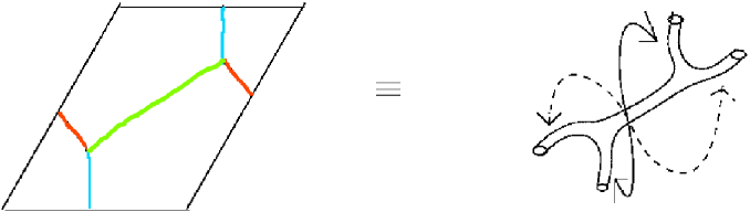
Figure 1: A dyon can be represented as a string web on a torus which in M-theory looks like a genus two Riemann surface.

The same conclusion can be reached by a slightly different reasoning in a single duality step within the heterotic description. For computing a partition function, we take time to be a Euclidean circle with supersymmetric boundary conditions. Both the fundamental string and the NS5-brane component extend along the euclidean time. We now have effectively, heterotic string on $T^{7}$ which has a larger U-duality group $O(8,24;\mathbb{Z})$ that combines together the T-duality group $O(7,23;\mathbb{Z})$ and the $SL(2,\mathbb{Z})$ S-duality group [30]. The chain of dualities described above can be condensed into a single U-duality transformation that sends the Euclidean NS5-branes wrapped along time to Euclidean fundamental strings that do not wrap the time circle, while at the same time leaving the fundamental strings wrapped along time unchanged. As a result, the partition function of quarter-BPS dyons is mapped to the partition function of a heterotic string worldsheet. The worldsheet has a component that wraps around time and one spatial direction, and another that wraps around the other two spatial directions, so that it wraps effectively a genus two curve.

Using this picture it is also easy to see why $\rho$, $\sigma$ and $v$ are the chemical potentials associated with $Q_{e}^{2}/2$, $Q_{m}^{2}/2$ , and $Q_{e}\cdot Q_{m}$ respectively. The genus-two momentum sum takes the form (25) with $(p^{i}_{L},p^{i}_{R})$ taking values in $\Gamma^{22,6}$ Narain lattice in the new heterotic frame. The momenta $(p^{1}_{L},p^{1}_{R})$ are identified with $Q_{e}$ of the original heterotic frame whereas the momenta $(p^{2}_{L},p^{2}_{R})$ are identified with $Q_{m}$. Integrating along $0\leq\textrm{Re}(\rho)\leq 1$, $0\leq\textrm{Re}(\sigma)\leq 1$, $0\leq\textrm{Re}(v)\leq 1$ as in [1] means $\Omega$ is real along the integration contour. From these facts it follows from the form of (25) that $\rho$, $\sigma$ and $v$ are the chemical potentials associated with $Q_{e}^{2}/2$, $Q_{m}^{2}/2$ , and $Q_{e}\cdot Q_{m}$ respectively.

So far we have been discussing the toroidally compactified case with $N=1$. For CHL orbifolds for other values of $N$, the genus-two worldsheet would have a branch cut of order $N$ along one of the cycles. This can be seen most easily in the string web picture. The CHL orbifold action combines an order $N$ shift $T$ along one of the circles with an order $N$ left-moving twist $\xi$ of the internal CFT. This implies that to construct a state wrapping a compact $T^{2}$ from the string web, two ends of the web in the fundamental cell of the $T^{2}$ along one of the cycles (shown in blue for example in Fig. 1) are joined after an order $N$ twist $\xi$. Using M-theory lift and heterotic dual as above, the resulting genus-two worldsheet then has a branch cut across which some of the left-moving fields undergo a $\mathbb{Z}_{N}$ twist. This will be explained more concretely for the $\mathbb{Z}_{2}$ case in the next section. Computation of the genus-two partition function will then reveal the correct Siegel modular form consistent with this picture.

4 Computation of the Twisted Chiral Partition Function

We would like to confirm the picture in the previous section with a computation of the genus-two partition function for CHL orbifolds for other values of $N>1$. We focus in this section on the $\mathbb{Z}_{2}$ CHL model where our computations can be carried through completely and where closed form expressions for $\Phi_{6}$ are available in terms of $\Phi_{10}$ and theta functions. This will allow for an explicit comparison of our computation with the proposed partition function. These considerations naturally generalize to other values of $N$.

To construct the $\mathbb{Z}_{2}$ CHL orbifold, one starts with a toroidally compactified $E_{8}\times E_{8}$ string which admits a $\mathbb{Z}_{2}$ left-moving symmetry generated by the element $\xi$ that flips the two $E_{8}$ factors. In the bosonic representation of the $E_{8}\times E_{8}$ current algebra, the first and the second $E_{8}$ factors can be represented by left-moving bosons $X^{I}$ and $Y^{I}$ respectively each living on the $E_{8}$ root lattice with $I=1,\ldots 8$. The combination $(X^{I}+Y^{I})/\sqrt{2}$ is then even under $\xi$ and $(X^{I}-Y^{I})/\sqrt{2}$ is odd. The CHL orbifolding action then combines this with a half-shift $T$ along $S^{1}$. We are interested in the genus-two chiral partition function of the left-moving bosons. The genus two worldsheet for the twisted sectors has a branch cut across which the fields $(X^{I}-Y^{I})/\sqrt{2}$ flip sign.

To evaluate the partition function of bosons on a genus $g$ Riemann surface with branch cuts, we closely follow the discussion in [31]. The partition function in this case can be written as a product of a classical piece and a quantum piece. The classical piece comes from a sum over instanton sectors of classical maps that have nontrivial windings around the target space and gives rise to a theta function over the Narain lattice. The quantum piece, which is usually the more difficult piece to evaluate, is determined in terms of the fluctuation determinants of the scalars as well as the ghosts. The bosonic determinants in general have complicated expressions and it is not easy to extract them in a useful form that can be compared with the Siegel modular forms. To circumvent this difficulty, we express the twisted partition function in terms of the untwisted partition function and theta functions. Since the total untwisted partition function is given as the inverse of the Igusa cusp form $\Phi_{10}$, we can then extract a closed form expression for the total twisted partition function. Our strategy will be to treat the quantum and classical pieces separately. We first evaluate the quantum piece and will later treat the classical piece that gives the lattice sum over charges. The two pieces individually have a dependence on Prym periods which cancels out from the final answer.

The quantum piece of the twisted theory can be obtained from the quantum piece of the untwisted theory by replacing eight untwisted bosonic determinants by eight twisted determinants,

$$Z^{qu}_{twisted}=Z^{qu}_{untwisted}\,(\frac{\Delta_{u}}{\Delta_{t}})^{8}.$$ (18)

Here $\Delta_{u}$ and $\Delta_{t}$ are the determinants over nonzero modes of the $\bar{\partial}$ operator on a genus two surface with untwisted and twisted boundary conditions across the branch cut respectively.

To evaluate the ratio of determinants, it is sufficient to consider a single scalar field $\varphi$ compactified on a circle of radius $R$ on a genus two Riemann surface $\Sigma$. We choose a canonical homology basis $(A_{i},B_{i})$, $i=1,2$ for the surface $\Sigma$, normalized with respect to the intersection product

$$\#(A_{i},A_{j})=\#(B_{i},B_{j})=0;\quad\#(A_{i},B_{j})=\#(B_{i},A_{j})=\delta_{ij}.$$ (19)

Note that linear relabeling of the homology cycles that leaves the intersection product invariant generates precisely the $Sp(2,\mathbb{Z})$ group of matrices defined in (5).

Let us first consider the unorbifolded theory of a scalar $\varphi$ on a circle, so that the Riemann surface $\Sigma$ has no branch cuts. The partition function is then given by the product of the classical and the quantum piece

$$Z_{\textrm{circle}}(R)=Z_{\textrm{circle}}^{cl}(R)Z_{\textrm{circle}}^{qu}\,.$$ (20)

The entire $R$ dependence is in the classical piece. Explicit form of the quantum part $Z^{qu}$ will not be needed for our purpose. The classical part is given by the partition sum over classical solutions $\partial\bar{\partial}\varphi^{cl}=0$ with winding numbers around various cycles. The nontrivial classical solutions can be written in terms of the integrals of the holomorphic one-forms $\omega_{i}=\omega_{i}(z)dz$ and their complex conjugates $\bar{\omega}_{i}=\bar{\omega}_{i}(\bar{z})d\bar{z}$, $i=1,2$. The holomorphic one-form are normalized with respect to the $A_{i}$ cycles and define the period matrix $\Omega$ by

$$\oint_{A_{i}}\omega_{j}=\delta_{ij}\qquad\oint_{B_{i}}\omega_{j}=\Omega_{ij}.$$ (21)

The winding numbers of $(l_{i},m_{i})$ the classical solution are defined by the periods

$$\oint_{A_{i}}d\varphi^{cl}=2\pi Rm_{i},\quad\oint_{B_{i}}d\varphi^{cl}=2\pi Rl_{i}.$$ (22)

A solution with given winding numbers can be written as

$$\varphi^{cl}(z)=-\frac{1}{2}\pi iR(l-\bar{\Omega}m)\cdot(\textrm{Im}\Omega)^{-1}\cdot\int_{z_{0}}^{z}\omega+\textrm{c}.\textrm{c},$$ (23)

with classical action

$$S[\varphi^{cl}]=\frac{1}{2}\pi R^{2}(m-\bar{\Omega}l)\cdot(\textrm{Im}\Omega)^{-1}\cdot(m-\Omega l).$$ (24)

Partition sum over these winding sectors then gives

$$Z^{cl}(R)=\sum_{(p_{L}^{i},p_{R}^{i})}\exp[\pi i(p_{L}\cdot\Omega\cdot p_{L}-p_{R}\cdot\bar{\Omega}\cdot p_{R})],$$ (25)

after Poisson resummation. The lattice sum can be interpreted as the sum over the left and right-moving momenta $\{p_{L}^{i},p_{R}^{i}\}$ flowing through each $B_{i}$ cycle. For each $i$, the momenta take values in self-dual Lorentzian Narain lattice $\Gamma^{1,1}$ spanned by

$$p^{i}_{R,L}=(\frac{n^{i}}{R}\pm\frac{w^{i}R}{2}).$$ (26)

We use the standard CFT conventions throughout so $\alpha^{\prime}=2$, the self-dual radius is $R=\sqrt{2}$, and the free field OPE are normalized $\phi(z)\phi(w)\sim-\ln(z-w)$.

In the orbifolded theory, the partition function is obtained by a functional integral over fields $\varphi$ which can be double-valued on $\Sigma$. These field configurations can be even or odd going around the four cycles $(A_{i},B_{i})$ and fall into $2^{4}$ distinct topological sectors corresponding to elements of $H_{1}(\Sigma,\mathbb{Z}_{2})$ labeled by the half-characteristics

$$\left[\begin{array}[]{c}\epsilon\\ \delta\end{array}\right]=\left[\begin{array}[]{c c}\epsilon_{1}&\epsilon_{2}\\ \delta_{1}&\delta_{2}\end{array}\right],\qquad(\epsilon_{i},\delta_{i}=0,\frac{1}{2}\,\,\textrm{for}\,\,i=1,2).$$ (27)

The orbifold partition function is then a sum over all sectors of the genus two surface,

$$Z_{\textrm{orbifold}}(R)=\frac{1}{2^{2}}\sum_{\epsilon,\delta}Z_{\epsilon,\delta}(R),$$ (28)

where $Z_{\epsilon,\delta}(R)$ is a partition sum over field configuration that are double valued across a branch cut along the cycle $\sum_{i}2(\delta_{i}A_{i}+\epsilon_{i}B_{i})$. As before, in each sector the partition sum is a product of a quantum piece and a classical piece.

$$Z_{\epsilon,\delta}(R)=Z^{qu}_{\epsilon,\delta}Z^{cl}_{\epsilon,\delta}(R)$$ (29)

The untwisted partition function $Z_{0,0}(R)$ is the partition function $Z_{\textrm{circle}}(R)$ of the circle theory that we have already evaluated above. For a nonzero characteristics, we can choose a new homology basis so that

$$\left[\begin{array}[]{c}\epsilon\\ \delta\end{array}\right]=\left[\begin{array}[]{c c}0&0\\ 0&\frac{1}{2}\end{array}\right].$$ (30)

which corresponds to choosing the branch cut around the new $A_{2}$ cycle. This branch cut defines a double cover ${\bf\pi}:\hat{\Sigma}\rightarrow\Sigma$ obtained by cutting the Riemann surface along the cycle $A_{2}$ and then pasting it with an identical copy which corresponds to the second Riemann sheet. The covering Riemann surface $\hat{\Sigma}$ is of genus three which is uniquely determined by the choice of the branch cut given a $\Sigma$. The double cover $\hat{\Sigma}$ admits a conformal involution ${\emph{i}}:\hat{\Sigma}\rightarrow\hat{\Sigma}$, satisfying $\pi\circ{\emph{i}}=\pi$, which basically interchanges the two Riemann sheets.

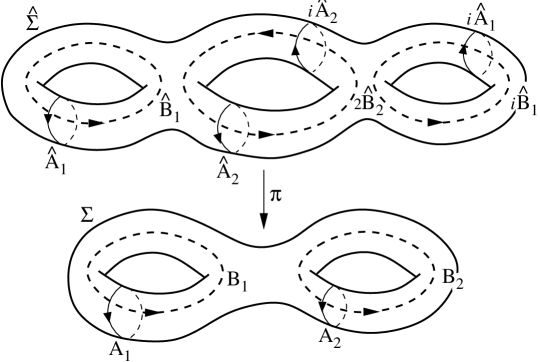
Figure 2: A double cover of a genus-two Riemann surface is a genus-three surface that admits an involution i.

A convenient choice for the homology basis on $\hat{\Sigma}$ is the one that projects on the homology basis of $\Sigma$. So it is given by $A_{1},B_{1};A_{2},2B_{2};{\emph{i}}(A_{1}),\emph{i}(B_{1})$. Given this double cover, one can define the Prym differential $\nu=\nu(\hat{z})d\hat{z}$ that is odd under the defining involution $\nu(\emph{i}(\hat{z}))=-\nu(\hat{z})$. They are normalized with respect to the A-cycles and defines the Prym period $\tilde{\tau}$ by,

$$\oint_{\hat{A}_{1}}\nu=-\oint_{\emph{i}(\hat{A}_{1})}\nu=1;\qquad\oint_{\hat{B}_{1}}\nu=-\oint_{\emph{i}(\hat{B}_{1})}\nu=\tilde{\tau}$$ (31)

The Prym differential has no periods around $\hat{A}_{2}$ and $2\hat{B}_{2}$. It is clear from the definition that the projection of the Prym differential on $\Sigma$ is a double valued holomorphic one-form which is antiperiodic around $B_{2}$. More generally, for a genus $g$ Riemann surface $\Sigma$, the double cover $\hat{\Sigma}$ is a Riemann surface of genus $(2g-1)$ and there are $(g-1)$ Prym differentials. Basically, the $(2g-1)$ holomorphic forms on the covering surface $\hat{\Sigma}$ can be split into even and odd under the automorphism. The $g$ even ones project down to the holomorphic differentials on $\Sigma$, the $(g-1)$ odd ones are the Prym differentials. The Prym periods in this case are a $(g-1)\times(g-1)$ matrix. For further details in this context see [31].

The twisted sector partition function on $\Sigma$ with the twist characteristic $(\epsilon,\delta)$ is then given by a functional integral over field configurations $\hat{\varphi}$ on the double cover $\hat{\Sigma}$ that are odd under the involution, $\hat{\varphi}(\emph{i}(\hat{z}))=-\hat{\varphi}(\hat{z})$ mod $2\pi R$. Because of the doubled area of $\hat{\Sigma}$, the action is halved compared to the standard normalization. The instanton configurations on the worldsheet $\hat{\Sigma}$ that contribute to the classical piece of the partition function are analogous to the untwisted ones and have the form

$$\varphi^{cl}(z)=-\frac{1}{2}\pi iR(l-\bar{\tilde{\tau}}m)(\textrm{Im}\tilde{\tau})^{-1}\int_{{\emph{i}}(\hat{z})}^{\hat{z}}\nu+\textrm{c}.\textrm{c}.$$ (32)

The twisted partition function in (29) then takes the form

$$Z_{\epsilon,\delta}(R)=Z^{qu}_{\epsilon,\delta}\sum_{(p_{L},p_{R})}\exp[\pi i(p_{L}\cdot{\tilde{\tau}_{\epsilon,\delta}}\cdot p_{L}-p_{R}\cdot\bar{\tilde{\tau}}_{\epsilon,\delta}\cdot p_{R})],$$ (33)

where the sum is over a single copy of the Narain lattice $\Gamma^{1,1}$ (26) and ${\tilde{\tau}}_{\epsilon,\delta}$ is the Prym period corresponding to the characteristic $(\epsilon,\delta)$.

Computing the quantum piece $Z^{qu}_{\epsilon,\delta}$ is much harder but it will suffice for our purposes to know the ratio of the quantum pieces for the twisted and untwisted bosons. This can be computed using the following trick that exploits the extra $SU(2)$ symmetry available for a free boson at the self-dual radius. The three $SU(2)$ currents $(J_{x},J_{y},J_{z})$ at $R=\sqrt{2}$ are given by $(\cos\sqrt{2}X,\sin\sqrt{2}X,\frac{1}{\sqrt{2}}\partial X)$. The $\mathbb{Z}_{2}$ orbifold action $X\to-X$ is a Weyl reflection that acts as a rotation through $\pi$ around the $x$ axis. This flips the sign of both $J_{y}$ and $J_{z}$ but leaves $J_{x}$ unchanged. This is clearly equivalent by $SU(2)$ conjugation to a rotation around the $z$ axis, which flips the sign of both $J_{x}$ and $J_{y}$ but leaves $J_{z}$ unchanged. Such a flip is achieved by a half shift on the circle $X\to X+\pi\sqrt{2}$. An orbifold by a half shift results in a circle conformal field theory at half the radius. Hence we have the equality between the orbifold CFT and the circle CFT as follows

$$Z_{\textrm{orbifold}}(R=\sqrt{2})=Z_{\textrm{circle}}(R=\frac{1}{\sqrt{2}}).$$ (34)

To use this equality effectively, it is convenient to write the non-holomorphic lattice sums in (25) and (33) as sums over holomorphically factorized chiral blocks. For this purpose, recall that a genus $g$ theta constants with characteristics are defined by

$$\vartheta\left[\begin{array}[]{cc}\alpha\\ \beta\\ \end{array}\right](\Omega)=\sum_{n\in\mathbb{Z}^{g}}\exp[i\pi(n+\alpha)\cdot\Omega\cdot(n+\alpha)+2\pi i(n+\alpha)\cdot\beta],$$ (35)

where the characteristics $\alpha$, $\beta$ are in general $g$-dimensional vectors and $\Omega$ is a $(g\times g)$ period matrix. When the radius $R^{2}/2$ is a rational number $p/q$, the momentum lattices appearing in (25) and (33) can be built up from a finite number of square sublattices. As a result, one can express the classical sum in (25) for example as

$$Z^{cl}(R) = \sum_{\alpha,\beta,\gamma}\vartheta\left[\begin{array}[]{c}\frac{1}{2}\alpha+\frac{1}{2}\beta+\gamma\\ 0\end{array}\right](2pq\Omega)\overline{\vartheta\left[\begin{array}[]{c}\frac{1}{2}\alpha-\frac{1}{2}\beta+\gamma\\ 0\end{array}\right](2pq\Omega)}$$ (40)

$$= 2^{-2}\sum_{\alpha,\beta,\gamma}e^{4\pi i\beta\cdot\gamma}\vartheta\left[\begin{array}[]{c}\alpha+\beta\\ \gamma\end{array}\right](\frac{1}{2}pq\Omega)\overline{\vartheta\left[\begin{array}[]{c}\alpha-\beta\\ \gamma\end{array}\right](\frac{1}{2}pq\Omega)},$$ (45)

where the summation is over $\alpha\in\left(\frac{1}{p}\mathbb{Z}_{p}\right)^{g}$, $\beta\in\left(\frac{1}{q}\mathbb{Z}_{q}\right)^{g}$, $\gamma\in(\frac{1}{2}(\mathbb{Z}_{2})^{g}$. Applying this formula to our cases of interest, we have

$$Z^{cl}_{\epsilon,\delta}(\sqrt{2})=\sum_{\alpha}\Bigg{|}\vartheta\left[\begin{array}[]{c}\alpha\\ 0\end{array}\right](2{\tilde{\tau}}_{\epsilon,\delta})\Bigg{|}^{2}$$ (46)

for the orbifold classical sum in (28) which depends on a genus-one Prym period ${\tilde{\tau}}_{\epsilon,\delta}$ and

$${Z^{cl}}_{\textrm{circle}}(\frac{1}{\sqrt{2}})=\frac{1}{2^{2}}\sum_{\alpha,\beta,\gamma}\Bigg{|}\vartheta\left[\begin{array}[]{c}\alpha+\frac{1}{2}\gamma\\ \beta\end{array}\right](2\Omega)\Bigg{|}^{2}$$ (47)

for the circle classical sum which depends on the genus-two period matrix $\Omega$. The equality (34) then reads

$$\frac{1}{2^{2}}\sum_{\epsilon,\delta,\gamma}Z^{qu}_{\epsilon,\delta}\Bigg{|}\vartheta\left[\begin{array}[]{c}\gamma\\ 0\end{array}\right](2\tilde{\tau}_{\epsilon,\delta})\Bigg{|}^{2}=\frac{1}{2^{2}}\sum_{\epsilon,\delta,\gamma}Z^{qu}_{0,0}\Bigg{|}\vartheta\left[\begin{array}[]{c}\frac{1}{2}\epsilon+\gamma\\ \delta\end{array}\right](2\Omega)\Bigg{|}^{2}\,.$$ (48)

A term by term comparison of the chiral blocks following the arguments in [31] then leads to the desired expression for the twisted determinant in terms of the untwisted determinant

$$Z^{qu}_{\epsilon,\delta}=\Bigg{|}c\left[\begin{array}[]{c}\epsilon\\ \delta\\ \end{array}\right]\Bigg{|}^{-2}Z^{qu}_{0},$$ (49)

with

$$c\left[\begin{array}[]{cc}0&0\\ 0&\frac{1}{2}\\ \end{array}\right]=\frac{\vartheta\left[\begin{array}[]{c}\gamma\\ 0\\ \end{array}\right](2{\tilde{\tau}})}{\vartheta\left[\begin{array}[]{cc}\gamma&0\\ 0&\frac{1}{2}\\ \end{array}\right](2\Omega)}.$$ (50)

For comparison with literature we use the notation $\vartheta_{abcd}={\vartheta\left[\begin{array}[]{cc}\frac{a}{2}&\frac{b}{2}\\ \frac{c}{2}&\frac{d}{2}\\ \end{array}\right]}$ and $\vartheta_{ab}={\vartheta\left[\begin{array}[]{c}\frac{a}{2}\\ \frac{b}{2}\\ \end{array}\right]}$. There are useful doubling identities for theta functions,

$$\vartheta^{2}_{10}(\tilde{\tau})=2\vartheta_{00}(2\tilde{\tau})\vartheta_{10}(2\tilde{\tau}),\quad\vartheta^{2}_{00}(\tilde{\tau})=\vartheta_{00}(2\tilde{\tau})^{2}+\vartheta_{10}(2\tilde{\tau})^{2},\quad\vartheta^{2}_{01}(\tilde{\tau})=\vartheta^{2}_{00}(2\tilde{\tau})-\vartheta^{2}_{10}(2\tilde{\tau}),$$ (51)

and similarly for the genus-two theta functions. Squaring or multiplying the two expressions for $c$ in (50) and rearranging them using doubling identities, we get other useful expressions

$$c^{2}\left[\begin{array}[]{cc}0&0\\ 0&\frac{1}{2}\\ \end{array}\right]=\frac{\vartheta^{2}\left[\begin{array}[]{c}\alpha\\ \beta\\ \end{array}\right]({\tilde{\tau}})}{\vartheta\left[\begin{array}[]{cc}\alpha&0\\ \beta&0\\ \end{array}\right](\Omega)\vartheta\left[\begin{array}[]{cc}\alpha&0\\ \beta&\frac{1}{2}\\ \end{array}\right](\Omega)},$$ (52)

that are available in [31]. Note that the left hand side is independent of the characteristics $\alpha$ and $\beta$. Equality of the right hand side for different choices of $\alpha$ and $\beta$ is the statement of the Schottky relations [31]. Using different values of $\alpha$ and $\beta$ we obtain

$$c^{2}_{0001}=\frac{\vartheta_{00}^{2}(\tilde{\tau})}{\vartheta_{0000}(\Omega)\vartheta_{0001}(\Omega)}=\frac{\vartheta_{01}^{2}(\tilde{\tau})}{\vartheta_{0010}(\Omega)\vartheta_{0011}(\Omega)}=\frac{\vartheta_{10}^{2}(\tilde{\tau})}{\vartheta_{1000}(\Omega)\vartheta_{1001}(\Omega)}\,.$$ (53)

Using these three equations we can write

$$\frac{1}{c^{8}_{0001}}=\frac{\vartheta_{0000}^{2}(\Omega)\vartheta_{0001}^{2}(\Omega)\vartheta_{0010}^{2}(\Omega)\vartheta_{0011}^{2}(\Omega)}{\vartheta_{00}^{4}(\tilde{\tau})\vartheta_{01}^{4}(\tilde{\tau})}\,,$$ (54)

$$\frac{1}{c^{8}_{0001}}=\frac{\vartheta_{0000}^{2}(\Omega)\vartheta_{0001}^{2}(\Omega)\vartheta_{1000}^{2}(\Omega)\vartheta_{1001}^{2}(\Omega)}{\vartheta_{00}^{4}(\tilde{\tau})\vartheta_{10}^{4}(\tilde{\tau})}\,,$$ (55)

$$\frac{1}{c^{8}_{0001}}=\frac{\vartheta_{1000}^{2}(\Omega)\vartheta_{1001}^{2}(\Omega)\vartheta_{0010}^{2}(\Omega)\vartheta_{0011}^{2}(\Omega)}{\vartheta_{10}^{4}(\tilde{\tau})\vartheta_{01}^{4}(\tilde{\tau})}\,.$$ (56)

These expressions are now in a convenient form to compare with the known expressions for $\Phi_{6}$ [32, 33]

$$\frac{1}{\Phi_{6}(\Omega)}=\frac{\vartheta_{0000}^{2}(\Omega)\vartheta_{0001}^{2}(\Omega)\vartheta_{0010}^{2}(\Omega)\vartheta_{0011}^{2}(\Omega)}{\Phi_{10}(\Omega)}\,,$$ (57)

$$\frac{1}{\Phi^{\prime}_{6}(\Omega)}=\frac{\vartheta_{0000}^{2}(\Omega)\vartheta_{0001}^{2}(\Omega)\vartheta_{1000}^{2}(\Omega)\vartheta_{1001}^{2}(\Omega)}{\Phi_{10}(\Omega)}\,,$$ (58)

$$\frac{1}{\Phi^{\prime\prime}_{6}(\Omega)}=\frac{\vartheta_{1000}^{2}(\Omega)\vartheta_{1001}^{2}(\Omega)\vartheta_{0010}^{2}(\Omega)\vartheta_{0011}^{2}(\Omega)}{\Phi_{10}(\Omega)}\,.$$ (59)

Here $\Phi_{6},\Phi^{\prime}_{6},\Phi^{\prime\prime}_{6}$ are various images of $\Phi_{6}$ under an $SL(2,\mathbb{Z})$ subgroup of the $Sp(2,\mathbb{Z})$ modular transformations. There are only three images because $\Phi_{6}$ is invariant under the subgroup $\Gamma_{0}(2)$ of index $3$ in $SL(2,\mathbb{Z})$.

To compare with (57), for example, one can multiply the expression (54) with the inverse power of $\Phi_{10}(\Omega)$. We therefore conclude that the quantum piece of the twisted chiral partition function of the left-moving heterotic string with the $\mathbb{Z}_{2}$ branch cut along the $A_{2}$ cycle is given by

$$\frac{\Delta^{8}_{0000}(\Omega)}{\Delta^{8}_{0001}(\Omega)}\frac{1}{\Phi_{10}(\Omega)}=\frac{1}{c^{8}_{0001}}\frac{1}{\Phi_{10}(\Omega)}=\frac{1}{\vartheta_{00}^{4}(\tilde{\tau})\vartheta_{01}^{4}({\tilde{\tau}})\Phi_{6}(\Omega)},$$ (60)

with similar expressions in terms of $\Phi^{\prime}_{6}$ and $\Phi^{\prime\prime}_{6}$. This is promising but still not quite right because there is an unwanted factor in the denominator involving theta functions over the Prym periods. As we will see below, these factors are eliminated once the classical contribution from the momentum sum is properly taken into account.

In the orbifolded theory, there are no gauge fields that couple to the odd $E_{8}$ charges. Nevertheless, states with these charges still run across the $B_{1}$ cycle of the genus two surface in Fig.2 that has no branch cut. Although we want to fix the momenta running along the two handles of the Riemann surface in terms of the electric and magnetic charges of the dyon, we still have to sum over the appropriate lattice of odd charges. The sum over the odd charges will give a theta function of the Prym period. We will show that it exactly cancels the theta function appearing in the denominator in (60).

The numerator for genus-two twisted partition function for the $\mathbb{Z}_{2}$ orbifold of the $E_{8}\times E_{8}$ lattice is a combination of expressions like (25) for the even momentum lattice and (33) for the odd momentum lattice. The lattice sum is best understood in terms of the covering genus-three surface $\hat{\Sigma}$. In the basis of cycles chosen earlier, it follows from the definition that the genus-three period matrix can be expressed in terms of genus-two quantities as

$$\hat{\Omega}=\left(\begin{array}[]{ccc}\frac{1}{2}(\rho+\tilde{\tau})&v&\frac{1}{2}(\rho-\tilde{\tau})\\ v&2\sigma&v\\ \frac{1}{2}(\rho-\tilde{\tau})&v&\frac{1}{2}(\rho+\tilde{\tau})\\ \end{array}\right).$$ (61)

Upon projection to $\Sigma$, the period matrix gives rise to the genus-two period matrix and the Prym period. The genus-three momentum sum over the $E_{8}\times E_{8}$ lattice $\Lambda$ is

$$\sum_{{\bf p}\in\Lambda^{3}}\exp{[\pi i({\bf p}\cdot\hat{\Omega}\cdot{\bf p})]}.$$ (62)

Given the form (61) of the period matrix, this expression can be reorganized in terms of genus-two objects as explained in appendix A to obtain ,

$$\Theta_{E8}(2\rho,2\sigma,2v)\vartheta^{4}_{00}({\tilde{\tau}})\vartheta^{4}_{01}({\tilde{\tau}})+\frac{1}{16}\Theta_{E8}(\frac{\rho}{2},2\sigma,v)\vartheta^{4}_{00}({\tilde{\tau}})\vartheta^{4}_{10}({\tilde{\tau}})-\frac{1}{16}\Theta_{E8}(\frac{\rho+1}{2},2\sigma,v)\vartheta^{4}_{01}({\tilde{\tau}})\vartheta^{4}_{10}({\tilde{\tau}}).$$

Combining this classical piece with the quantum twisted determinants that we have calculated earlier, we see that the dependence on Prym periods cancels completely. The full twisted partition function is then

$$Z_{twisted}=\frac{\Theta_{E8}(2\rho,2\sigma,2v)}{\Phi_{6}(\Omega)}+\frac{1}{16}\frac{\Theta_{E8}(\frac{\rho}{2},2\sigma,v)}{\Phi^{\prime}_{6}(\Omega)}-\frac{1}{16}\frac{\Theta_{E8}(\frac{\rho+1}{2},2\sigma,v)}{\Phi^{\prime\prime}_{6}(\Omega)}.$$ (63)

Here we have suppressed the uninteresting momentum sum coming from the toroidal compactification.

Recall that the proposal of [2] gives the dyon partition function for a specific class of states, which carry half-integral units of winding along the CHL circle. Comparison with the genus one partition function for electric states computed for example in [22] shows that the states that carry half a unit of winding on the CHL circle are associated with the even $E_{8}$ charges contained in $\Theta_{E8}(\rho/2,2\rho,v)$. Hence we reproduce the result that the corresponding degeneracies are the Fourier coefficients of $-1/16{\Phi^{\prime}_{6}(\Omega)}$. Comparing the expression for $C$ in (13) for $N=1$ and $N=2$, we see that we also correctly reproduce the normalization relative to the $N=1$ case.

This concludes the main part of the derivation. The Igusa cusp form $\Phi_{10}$ is proportional to the product of all ten genus-two theta functions with even spin structure,

$$\Phi_{10}(\Omega)=2^{-12}\prod_{{\alpha,\beta}\atop 4\alpha\cdot\beta=even}\vartheta^{2}\left[\begin{array}[]{cc}\alpha\\ \beta\\ \end{array}\right](\Omega).$$ (64)

This allows us to express $\Phi_{6}$ using (57) as a product of six particular even theta functions

$$\Phi_{6}=2^{-12}(\vartheta_{0100}\vartheta_{0110}\vartheta_{1000}\vartheta_{1001}\vartheta_{1100}\vartheta_{1111})^{2},$$ (65)

Our results can thus be viewed as a CFT derivation of the level 2 Siegel modular form $\Phi_{6}$ in terms of theta functions that was obtained by Ibukiyama from a very different starting point [32, 33].

A few comments are in order. First, let us make the modular properties of $\Phi_{6}(\Omega)$ under $G_{0}(2)$ more manifest. The theta function in the numerator, $\Theta_{E8}(2\Omega)$ is clearly modular under $G_{0}(2)$. Note that $G_{0}(2)$ consists of matrices of the form (5) with $C=2C^{\prime}$ for some integral $C^{\prime}$. Defining $B^{\prime}=2B$ we see that under $G_{0}(2)$ transformation the theta function transforms as

$$\Theta_{E8}(2\Omega)\rightarrow\Theta_{E8}(2\frac{A\Omega+B}{C\Omega+D})=\Theta_{E8}(\frac{A2\Omega+B^{\prime}}{C^{\prime}2\Omega+D})$$ (66)

Since $\Theta_{E8}(\Omega)$ is modular under $SP(2,\mathbb{Z})$, it follows that $\Theta_{E_{8}}(\frac{A2\Omega+B^{\prime}}{C^{\prime}2\Omega+D})$ can be reexpressed in terms of $\Theta_{E_{8}}(2\Omega)$. We then conclude that $\Theta_{E_{8}}(2\Omega)$ is modular under $G_{0}(2)$. Now, the sum of the partition functions for all twisted sectors is modular invariant under $Sp(2,Z)$. The theta function $\Theta_{E8}(2\Omega)$ will appear in several sectors, as $Z_{0001}$ or $Z_{0010}$, etc. By inspection, one can also see that it always appears accompanied by $\Phi_{6}(\Omega)$ in the denominator. The sum of all partition functions will then be a sum of various modular images of $\Theta_{E8}(2\rho,2\sigma,2v)$ over $\Phi_{6}$ as in (63). For this to be invariant under $Sp(2,\mathbb{Z})$, and since the theta function in the numerator is modular under $G_{0}(2)$, the denominators must be $G_{0}(2)$ modular forms as well. Hence $\Phi_{6}(\Omega)$ must a modular form for $G_{0}(2)$. This derivation also makes clear why the larger $G_{0}(2)$ appears even though the subgroup $G_{1}(2)$ is adequate for accommodating the S-duality group $\Gamma_{1}(2)$.

Second, the precise cancelations of the Prym parameters that made this result possible appear mysterious at first sight. However this is not an accident but rather a consequence of the equivalence of the $E_{8}\times E_{8}$ and of the $(E_{8}\times E_{8})/{\mathbb{Z}_{2}}$ CFTs. This fact suggests another way to derive the required Siegel modular forms which will be outlined in appendix B.

5 Generalization to $\mathbb{Z}_{N}$ Orbifolds

For higher $\mathbb{Z}_{N}$ orbifolds, the explicit CFT computations are more complicated. For instance, the left-moving twist symmetry $\xi$ is more involved for general $N$. However, using our experience with the $\mathbb{Z}_{2}$ orbifold, we can streamline our derivation and point out some of the essential ingredients in the general $\mathbb{Z}_{N}$ case.

The dyon partition function of a $\mathbb{Z}_{N}$ CHL orbifold is given in terms of the Siegel modular form $\Phi_{k}$. These forms are defined by their modular properties and behavior at the boundary of moduli space. No expression in terms of theta functions is available but a CFT derivation along the lines outlined here will result in such an expression. For now, one proceed indirectly and argue that the genus two chiral partition function for the CHL orbifold involves a modular form with the same modular properties and value at the boundary of moduli space as $\Phi_{k}$. There is no uniqueness theorem proven for these forms however it is likely that they are unique. Note that the form $\Phi_{k}$ is obtained by an additive lift of the form $f_{k}(\tau)=\eta^{k+2}(\tau)\eta^{k+2}(N\tau)$ which is known to be the unique cusp form of $\Gamma_{1}(N)$. We will also argue that $\Phi_{k}$ have a nice expression in terms of theta functions.

Let us recall some facts about a $\mathbb{Z}_{N}$ CHL orbifold. The orbifold is defined in terms of a $\mathbb{Z}_{N}$ action on $N$ groups of $l$ left-moving bosons. If we diagonalize the $\mathbb{Z}_{N}$ action then it is clear that $l$ bosons are left invariant and the remaining $l(N-1)$ bosons transform nontrivially. As a result, $l(N-1)$ left-moving gauge fields are projected out and the rank is reduced by $m=l(N-1)$ units. Starting with rank $28$ for the toroidally compactified case, we thus obtain a model with a reduced rank $r=28-l(N-1)$. From the list of known CHL models for $N=2,3,5,7$ to four dimensions that have $r=20,16,12,10$ we conclude that $l=8,6,4,3$. We would now like to see how the weight $k$ of the relevant Siegel modular form can be derived from this data using the underlying picture of genus-two worldsheet.

To implement such a $\mathbb{Z}_{N}$ symmetry, one would have to start with a self-dual Narain lattice $\Lambda$ of the form $\Gamma^{(lN,lN-16)}$ which contains a sublattice $\Lambda_{0}$ of the form $\Gamma^{(l,lN-16)}$ fixed by the $\mathbb{Z}_{N}$ action and an orthogonal left-moving complement $\Lambda_{1}$ of the form $\Gamma^{(l(N-1),0)}$ that is rotated by the left-moving $\mathbb{Z}_{N}$ action. Such a choice reduces the rank by $l(N-1)$ because gauge fields associated with the $\Lambda_{1}$ lattice are eliminated. The lattice $\Lambda_{1}$ is strongly constrained by the requirement of modular invariance and $\mathbb{Z}_{N}$ action.

The computation of the twisted partition function proceeds as in the $\mathbb{Z}_{2}$ case. The quantum piece of the $\mathbb{Z}_{N}$ orbifold twisted determinant can be computed from properties of $SU(N)$ WZW model at level one by using the fact that $\mathbb{Z}_{N}$ orbifold symmetry can be viewed as a Weyl symmetry of the $SU(N)$. Thus, by $SU(N)$ conjugation, an order $N$ twist can again be viewed as an order $N$ shift along the lattice. Using this trick, the ratio between twisted and untwisted determinants can be written again in terms of theta functions at genus one. At genus two it can be written in $N$ different ways as a ratio between a twisted $SU(N)$ theta function of the modular matrix and a $SU(N)$ theta function of the Prym period.

Now, we have seen that the dependence on the Prym period cancels out in the $\mathbb{Z}_{2}$ case in an apparently magical fashion from the final expression for the partition function. This cancelation was essential to obtain a nice Siegel modular form in the final answer and was not an accident. In the $\mathbb{Z}_{2}$ case, it is a consequence of the fact that orbifolding by $\xi$ alone without accompanying it with the shift $T$ along the circle leads back to the original theory leading to the identity (75) and its generalization to higher genera. We expect this to be true even in the $\mathbb{Z}_{N}$. Otherwise, it would lead to an undesirable dependence on the Prym periods. Such a computation would provide a useful representation of these forms $\Phi_{k}$ in terms of theta functions.

With this information we can deduce the weight of the relevant Siegel modular form quite easily. Basically, the point is that the twisted sector partition function is short of a lattice sum over $\Lambda_{1}$ in the numerator. A momentum sum over the $m$ dimensional lattice would have led to a theta function with modular weight $m/2$ which would now be missing. To compensate for this, the twisted determinants in the denominator should also have a correspondingly smaller weight. Putting all factors together we get the modular form $\Phi_{10}$ of weight $10$ in the denominator of the untwisted partition sum. Hence we expect that the modular form in the denominator in the twisted sector will have weight $k=(10-m/2)$. Substituting $l(N+1)=24$ and $m=l(N-1)$, we obtain $k=(l-2)$ or $k=24/(N+1)-2$ precisely in agreement with the proposed relation (9). Note that in [2], the relation between $k$ and $N$ was put in by hand to obtain agreement with the subleading terms in the Bekenstein-Hawking-Wald entropy. Here we are able to derive it from general considerations of the genus-two partition function of the orbifold. We have summarized various parameters of the orbifolds in the table (9).

N	l	k	r	m	$\Lambda_{0}$	$\Lambda_{1}$	$\Lambda$
2	8	6	20	8	$\Gamma^{(8,0)}$	$\Gamma^{(8,0)}$	$\Gamma^{(16,0)}$
3	6	4	16	12	$\Gamma^{(6,2)}$	$\Gamma^{(12,0)}$	$\Gamma^{(18,2)}$
5	4	2	12	16	$\Gamma^{(4,4)}$	$\Gamma^{(16,0)}$	$\Gamma^{(20,4)}$
7	3	1	10	18	$\Gamma^{(3,5)}$	$\Gamma^{(18,0)}$	$\Gamma^{(21,5)}$

Table 1: List of parameters for available CHL Orbifolds

Note that the $\mathbb{Z}_{7}$ orbifold is qualitatively different since it requires a $(21,5)$ lattice and thus one does not a fully factorized $K3\times T^{2}$ that was necessary to use the string web picture. It is possible therefore that this case requires a slightly different treatment.

6 Comments

We conclude with a brief comment on the fermionic zero modes. We have not dealt with the right-moving superstring carefully. Effectively, our prescription was to evaluate the genus two partition function of the bosonic string and then use holomorphic factorization to read off the left-moving part. It should be possible to define an intrinsically superstring amplitude. For example, in the Green-Schwarz formalism, the full partition function vanishes because of the fermion zero modes but an insertion of an appropriate number of fermionic currents can soak up the right-moving fermion zero modes. The nonzero modes of the Green-Schwarz fermions and the light-cone bosons are expected to cancel in pairs in the right-moving partition function leaving behind only the left-moving partition function. This would correspond to an appropriate index-like quantity such as a helicity supertrace. Such a prescription surely works at genus-one to correctly obtain the helicity supertrace that counts the heterotic half-BPS states. At genus two, the Green-Schwarz superstring is more subtle but it would be desirable to have an appropriate definition of index-like quantity that is non-vanishing after soaking up the zero modes and counts the left-moving fluctuations.

The genus-two picture outlined here is easily amenable to generalizations to other more general orbifolds [34, 35]. These generalizations and an elaboration of the computation outlined in appendix (B) will be explored elsewhere. The genus two picture also raises the question of possible contributions of higher genus surfaces. This question will be addressed in the forthcoming publication [4].

Acknowledgements

We would like to thank Ashoke Sen and Herman Verlinde for useful discussions. A. D. would like to thank Harvard University, LPTHE at the University of Paris, and Aspen Center for Physics for hospitality where part of this work was completed. D. G. would like to thank TIFR for hospitality where this work was initiated.

Appendix A Computation of the Classical Piece of the Partition Function

The classical piece coming from the sum over momenta involving the period matrix $\Omega$ and the Prym period $\tilde{\tau}$ is best understood in terms of the period matrix of the covering space $\hat{\Sigma}$ of genus-three. The genus-three theta function for an $E_{8}$ factor (62) involves a sum over momenta ${\bf p}=(p_{1},p_{2},p_{3})$ where each momentum $p_{i}$ takes values in the $E_{8}$ root lattice $\Lambda$ with length-squared two. Using the specific form of the period matrix for $\hat{\Sigma}$ in (61) we can write it in terms of genus-two objects as

$$\sum_{p_{1},p_{2},p_{3}\in\Lambda}\exp\left[\pi i{\frac{p_{1}+p_{3}}{\sqrt{2}}\choose\sqrt{2}p_{2}}\cdot\Omega\cdot{\frac{p_{1}+p_{3}}{\sqrt{2}}\choose\sqrt{2}p_{2}}\right]\times\exp\left[\pi i\frac{p_{1}-p_{3}}{\sqrt{2}}\cdot\tilde{\tau}\cdot\frac{p_{1}-p_{3}}{\sqrt{2}}\right]\,\,.$$ (67)

The vector $\sqrt{2}p_{2}$ lies in the “level two” lattice $\Lambda[2]$ which is a lattice with twice as large length-squared compared to $\Lambda$. The vectors $({p_{1}+p_{3}})/\sqrt{2}$ are in a copy of $\Lambda[2]$ shifted by some element ${\cal P}$ in the coset $\Lambda[2]^{*}/\Lambda[2]$, $({p_{1}-p_{3}})/\sqrt{2}$ in another copy of $\Lambda[2]$ shifted by the same ${\cal P}$. In the specific example of $\Lambda$ being the lattice of $E_{8}$, there are $256$ values of ${\cal P}$, collected into orbits of the Weyl group of the fundamental weight of the trivial, adjoint, and 3875 representations, of lengths 1, 120, and 135, respectively [22]. This allows one to reorganize the expression above as

$$\sum_{{\cal P}\in\frac{\Lambda}{2\Lambda}}\left(\sum_{q_{1}\in\Lambda[2]\atop q_{2}\in\Lambda[2]+{\cal P}}\exp\left[\pi i{q_{1}\choose q_{2}}\cdot\Omega\cdot{q_{1}\choose q_{2}}\right]\times\sum_{q_{3}\in\Lambda[2]+{\cal P}}\exp\left[\pi iq_{3}\cdot\tilde{\tau}\cdot q_{3}\right]\right),$$ (68)

The momentum sum involving the Prym period can be readily performed. It is useful to introduce $E_{8}$ theta functions with characteristics:

$$\Theta_{E_{8}[2],{\cal P}}({\tilde{\tau}}):=\sum_{\Delta\in E_{8}(1)}e^{2\pi i{\tilde{\tau}}(\Delta-\frac{1}{2}{\cal P})^{2}}$$ (69)

The theta series are thus the numerators of affine characters of $E_{8}$ at level 2, and can be computed explicitly using free fermion representations or by inspection in the bosonic representation [22]:

$$\begin{array}[]{lcccc}\Theta_{E_{8}[2],1}({\tilde{\tau}})&=&\Theta_{E_{8}[1]}(2{\tilde{\tau}})&=&\frac{1}{16}(\vartheta_{3}^{4}\vartheta_{2}^{4}-\vartheta_{4}^{4}\vartheta_{2}^{4}+16\vartheta_{3}^{4}\vartheta_{4}^{4})\\ \Theta_{E_{8}[2],248}({\tilde{\tau}})&=&\frac{1}{2}\left(\theta_{3}^{6}\theta_{2}^{2}+\theta_{2}^{6}\theta_{3}^{2}\right)(2{\tilde{\tau}})&=&\frac{1}{16}(\vartheta_{3}^{4}\vartheta_{2}^{4}+\vartheta_{4}^{4}\vartheta_{2}^{4})\\ \Theta_{E_{8}[2],3875}({\tilde{\tau}})&=&\theta_{3}^{4}\theta_{2}^{4}(2{\tilde{\tau}})&=&\frac{1}{16}(\vartheta_{3}^{4}\vartheta_{2}^{4}-\vartheta_{4}^{4}\vartheta_{2}^{4})\end{array}$$ (70)

Note that the combination $\vartheta_{3}^{4}\vartheta_{4}^{4}$ appears only in $\Theta_{E_{8}[2],1}$ corresponding to ${\cal P}=0$. Hence the coefficient of $\vartheta_{3}^{4}\vartheta_{4}^{4}$ is just

$$\sum_{q_{1}\in\Lambda[2]\atop q_{2}\in\Lambda[2]}\exp\left[\pi i{q_{1}\choose q_{2}}\cdot\Omega\cdot{q_{1}\choose q_{2}}\right]=\Theta_{E8}(2\rho,2\sigma,2v).$$ (71)

Similarly, the combination $\vartheta_{3}^{4}\vartheta_{2}^{4}$ appears for all three classes of $\cal P$ in (70) with the same coefficient. Thus, in (67) we now have the sum over $q_{2}$ taking values in $\Lambda[2]+\cal P$ with an unrestricted sum over $\cal P$. We can thus replace these two sum by a single sum over $q_{2}$ that takes values in $\Lambda^{*}$. As a result, the coefficient of $\vartheta_{3}^{4}\vartheta_{2}^{4}$ is simply

$$\frac{1}{16}\sum_{q_{1}\in\Lambda[2]\atop q_{2}\in\Lambda[2]^{*}}\exp\left[\pi i{q_{1}\choose q_{2}}\cdot\Omega\cdot{q_{1}\choose q_{2}}\right]=\frac{1}{16}\Theta_{E8}(\frac{\rho}{2},2\sigma,v).$$ (72)

By a similar reasoning, the coefficient of $\vartheta_{4}^{4}\vartheta_{2}^{4}$ is

$$-\frac{1}{16}\sum_{q_{1}\in\Lambda[2]\atop q_{2}\in\Lambda[2]^{*}}(-1)^{q_{2}^{2}}\exp\left[\pi i{q_{1}\choose q_{2}}\cdot\Omega\cdot{q_{1}\choose q_{2}}\right]=-\frac{1}{16}\Theta_{E8}(\frac{\rho+1}{2},2\sigma,v).$$ (73)

Here the term $(-1)^{q_{2}^{2}}$ accounts for the fact that the $248$ representation has relative minus sign with respect to the other two representations for the coefficient of $\vartheta_{4}^{4}\vartheta_{2}^{4}$ in (70). Putting it together we see that the momentum sum (62) equals

$$\Theta_{E8}(2\rho,2\sigma,2v)\vartheta^{4}_{00}({\tilde{\tau}})\vartheta^{4}_{01}({\tilde{\tau}})+\frac{1}{16}\Theta_{E8}(\rho/2,2\sigma,v)\vartheta^{4}_{00}({\tilde{\tau}})\vartheta^{4}_{10}({\tilde{\tau}})-\frac{1}{16}\Theta_{E8}(\frac{\rho+1}{2},2\sigma,v)\vartheta^{4}_{01}({\tilde{\tau}})\vartheta^{4}_{10}({\tilde{\tau}}).$$

Appendix B An Outline of An Alternative Derivation

It is well-known that if we take the orbifold generator to be $\xi$ alone without the half-shift $T$ along the circle, then the resulting orbifold gives back the same theory. The twisted sectors have integral conformal dimensions, and neatly take the place of the odd $E_{8}$ currents that are removed by the orbifolding projection. This equivalence suggests another way to derive the expression for $\Phi_{6}$ in terms of $\Phi_{10}$ and theta function.

For simplicity, let us first consider the genus-one case. The above equivalence implies in particular the equality of the torus partition function of the two theories

$$\frac{\Theta^{2}_{E8}({\tau})}{\eta^{16}({\tau})}=\frac{1}{2}\frac{\Theta^{2}_{E8}({\tau})}{\eta^{16}({\tau})}+\frac{1}{2}\frac{\Theta_{E8}(2{\tau})}{\eta^{8}(2{\tau})}+\frac{1}{2}\frac{\Theta_{E8}(\frac{{\tau}}{2})}{\eta^{8}(\frac{{\tau}}{2})}+\frac{1}{2}\frac{\Theta_{E8}(\frac{{\tau}+1}{2})}{\eta^{8}(\frac{{\tau}+1}{2})}$$ (74)

By some simple $\vartheta$ identities this can be rewritten as a useful theta function equality

$$\Theta^{2}_{E8}(\tau)=\Theta_{E8}(2\tau)\vartheta^{4}_{00}(\tau)\vartheta^{4}_{10}(\tau)+\Theta_{E8}(\frac{{\tau}}{2})\vartheta^{4}_{00}({\tau})\vartheta^{4}_{10}({\tau})-\Theta_{E8}(\frac{{\tau}+1}{2})\vartheta^{4}_{01}({\tau})\vartheta^{4}_{10}({\tau}).$$ (75)

This identify implies

$$\frac{\Theta^{2}_{E8}(\tau)}{\eta^{24}(\tau)}=\frac{\Theta_{E8}(2\tau)}{\eta^{8}(\tau)\eta^{8}(2\tau)}+\ldots$$ (76)

Note that $\eta^{24}$ is the genus-one analog of $\Phi_{10}$ whereas $\eta^{8}(\tau)\eta^{8}(2\tau)$ is the genus-one analog of $\Phi_{6}$ associated with the counting of electric states. We therefore expect a similar identity for the genus two partition function which follows from the above equivalence of orbifolded and unorbifolded theory. It should read

$$\Theta^{2}_{E8}(\Omega)=\Theta_{E8}(2\Omega)\vartheta_{0000}^{2}(\Omega)\vartheta_{0001}^{2}(\Omega)\vartheta_{0010}^{2}(\Omega)\vartheta_{0011}^{2}(\Omega)+\cdots$$ (77)

$$\frac{\Theta^{2}_{E8}(\Omega)}{\Phi_{10}(\Omega)}=\frac{\Theta_{E8}(2\Omega)}{\Phi_{6}(\Omega)}+\cdots$$ (78)

This expression has to coincide with the sum of all the twisted partition functions $Z_{abcd}$. It clearly does not involve any explicit dependence on the Prym parameters, and indicates that the dependence should drop off the single $Z_{abcd}$ as well. It also motivates more directly the expression of $\Phi_{6}$ in terms of theta functions. We expect that these ideas can be generalized to the general $\mathbb{Z}_{N}$ orbifolds.

References

- [1] R. Dijkgraaf, E. P. Verlinde, and H. L. Verlinde, Counting dyons in n = 4 string theory, Nucl. Phys. B484 (1997) 543–561, [hep-th/9607026].
- [2] D. P. Jatkar and A. Sen, Dyon spectrum in chl models, hep-th/0510147.
- [3] G. Lopes Cardoso, B. de Wit, J. Kappeli, and T. Mohaupt, Asymptotic degeneracy of dyonic n = 4 string states and black hole entropy, JHEP 12 (2004) 075, [hep-th/0412287].
- [4] A. Dabholkar, D. Gaiotto, and S. Nampuri, Comments on the dyon spectrum in n =4 compactifications, to appear.
- [5] J. Igusa, On siegel modular varieties of genus two, Amer. J. Math. 84 (1962) 175–200.
- [6] J. Igusa, On siegel modular varieties of genus two (ii), Amer. J. Math. 86 (1962) 392–412.
- [7] D. Gaiotto, Re-recounting dyons in n = 4 string theory, hep-th/0506249.
- [8] A. Dabholkar and S. Nampuri, Spectrum of dyons and black holes in chl orbifolds using borcherds lift, hep-th/0603066.
- [9] D. Gaiotto, A. Strominger, and X. Yin, New connections between 4d and 5d black holes, hep-th/0503217.
- [10] D. Shih, A. Strominger, and X. Yin, Recounting dyons in n = 4 string theory, hep-th/0505094.
- [11] J. R. David and A. Sen, Chl dyons and statistical entropy function from d1-d5 system, hep-th/0605210.
- [12] J. R. David, D. P. Jatkar, and A. Sen, Product representation of dyon partition function in chl models, hep-th/0602254.
- [13] S. Chaudhuri, G. Hockney, and J. D. Lykken, Maximally supersymmetric string theories in d ¡ 10, Phys. Rev. Lett. 75 (1995) 2264–2267, [hep-th/9505054].
- [14] S. Chaudhuri and J. Polchinski, Moduli space of chl strings, Phys. Rev. D52 (1995) 7168–7173, [hep-th/9506048].
- [15] S. Chaudhuri and D. A. Lowe, Type iia heterotic duals with maximal supersymmetry, Nucl. Phys. B459 (1996) 113–124, [hep-th/9508144].
- [16] J. H. Schwarz and A. Sen, Type iia dual of the six-dimensional chl compactification, Phys. Lett. B357 (1995) 323–328, [hep-th/9507027].
- [17] C. Vafa and E. Witten, Dual string pairs with n = 1 and n = 2 supersymmetry in four dimensions, Nucl. Phys. Proc. Suppl. 46 (1996) 225–247, [hep-th/9507050].
- [18] P. S. Aspinwall, Some relationships between dualities in string theory, Nucl. Phys. Proc. Suppl. 46 (1996) 30–38, [hep-th/9508154].
- [19] A. Sen, Entropy function for heterotic black holes, hep-th/0508042.
- [20] M. Eichler and D. Zagier, The theory of jacobi forms, Birkhauser (1985).
- [21] A. Dabholkar, F. Denef, G. W. Moore, and B. Pioline, Exact and asymptotic degeneracies of small black holes, JHEP 08 (2005) 021, [hep-th/0502157].
- [22] A. Dabholkar, F. Denef, G. W. Moore, and B. Pioline, Precision counting of small black holes, hep-th/0507014.
- [23] A. Sen, Black holes, elementary strings and holomorphic anomaly, JHEP 07 (2005) 063, [hep-th/0502126].
- [24] A. Dabholkar and J. A. Harvey, Nonrenormalization of the superstring tension, Phys. Rev. Lett. 63 (1989) 478.
- [25] A. Dabholkar, G. W. Gibbons, J. A. Harvey, and F. Ruiz Ruiz, Superstrings and solitons, Nucl. Phys. B340 (1990) 33–55.
- [26] O. Aharony, A. Hanany, and B. Kol, Webs of (p,q) 5-branes, five dimensional field theories and grid diagrams, JHEP 01 (1998) 002, [hep-th/9710116].
- [27] A. Sen, String network, JHEP 03 (1998) 005, [hep-th/9711130].
- [28] G. W. Moore, Modular forms and two loop string physics, Phys. Lett. B176 (1986) 369.
- [29] A. A. Belavin, V. Knizhnik, A. Morozov, and A. Perelomov, Two and three loop amplitudes in the bosonic string theory, JETP Lett. 43 (1986) 411.
- [30] A. Sen, Strong - weak coupling duality in three-dimensional string theory, Nucl. Phys. B434 (1995) 179–209, [hep-th/9408083].
- [31] R. Dijkgraaf, E. P. Verlinde, and H. L. Verlinde, C = 1 conformal field theories on riemann surfaces, Commun. Math. Phys. 115 (1988) 649–690.
- [32] T. Ibukiyama, On siegel modular varieties of level 3, Int. J. Math 2(1) (1991) 17–35.
- [33] H. Aoki and T. Ibukiyama, Simple graed rings of siegel modular forms, differential operators and borcherds products, International Journal of Mathematics 16 (2005) 249–279.
- [34] J. R. David, D. P. Jatkar, and A. Sen, Dyon spectrum in n = 4 supersymmetric type ii string theories, hep-th/0607155.
- [35] J. R. David, D. P. Jatkar, and A. Sen, Dyon spectrum in generic n = 4 supersymmetric z(n) orbifolds, hep-th/0609109.