On Hamiltonian approach to Standard Model

Abstract

The vector bosons models including Standard Model (SM) are investigated in the framework of the Dirac Hamiltonian method with explicit resolving the Gauss constraints in order to eliminate variables with zero momenta and negative energy contributions in accordance with the operator quantization principles. The Hamiltonian formulation admits the dynamic version of the Higgs potential, where its constant parameter is replaced by the dynamic zero Fourier harmonic of the very Higgs field. In this case, the zero mode equation is a new sum-rule that predicts mass of Higgs field $m_{h}=\sqrt{6m^{2}_{t}-4[2M_{W}^{2}+M_{Z}^{2}]}=311.6\pm 8.9\mbox{\rm GeV}$. The Hamiltonian formulation leads to static interactions playing the crucial role in the off-mass-shell phenomena of the type of bound state and a kaon - pion transition in the weak nonleptonic decays.

12.15.-y, 11.15.-q, 11.15.Ex, 11.30.Qc, 14.80.Bn, 14.70.Fm, 14.70.Hp, 14.65.Ha, 14.70.-e, 12.39.Fe

1 Introduction

The Hamiltonian approach to gauge theories was considered as the mainstream of development of gauge theories beginning with the pioneer papers by Dirac [1], Heisenberg and Pauli [2], and finishing by the Schwinger quantization of the non-Abelian theory [3] (see in detail [4, 5]). They postulated the higher priority of the quantum principles, in particular, in accordance with the uncertainty principle, one counted that we cannot quantize ”field variables” whose velocities are absent in the Lagrangian. Therefore, vector field time components with negative contributions into energy are eliminated, as it was accepted in the Dirac approach to QED [1]. This illumination leads to the static interactions and instantaneous bound states.

Remember that the Dirac Hamiltonian approach generalized to the non-Abelian theory [3, 5] and the massive vector fields [6] provides the fundamental operator quantization and correct relativistic transformations of states of quantized fields. This Hamiltonian approach is considered [7] as the foundation of all heuristic methods of quantization of gauge theories, including the Faddeev-Popov (FP) method [8] used now for description of Standard Model of elementary particles [9]. Moreover, Schwinger … rejected all Lorentz gauge formulations as unsuited to the role of providing the fundamental operator quantization (see [3] p.324). However, a contemporary reader could not find the Hamiltonian presentation of the Standard Model (SM) because there is the opinion [7] that this presentation is completely equivalent to the accepted version of SM based on the FP method [9].

In this paper, the Weinberg–Salam Standard Model is studied in the framework of the Dirac Hamiltonian method with explicit resolving the Gauss constraints in order to eliminate variables with zero momenta and negative contribution in energy. We try to reply the following question. What are new physical results that following from the Hamiltonian approach to QED and SM?

2 Hamiltonian approach to QED

2.1 Action and reference frame

Let us recall the Dirac approach [1] to QED. The theory is given by the well known action

$$S=\int d^{4}x\bigg{\{}-\frac{1}{4}F_{\mu\nu}F^{\mu\nu}+\bar{\psi}[i\hbox to0.0pt{/\hss}\partial-m]\psi+A_{\mu}j^{\,\mu}\bigg{\}},$$ (1)

where $F_{\mu\nu}=\partial_{\mu}A_{\nu}-\partial_{\nu}A_{\mu}$ is a tension, $A_{\mu}$ is a vector potential, $\psi$ is the Dirac electron-positron bispinor field and $j_{\mu}=e\bar{\psi}\gamma_{\mu}\psi$ is the charge current and $\hbox to0.0pt{/\hss}\partial=\partial^{\mu}\gamma_{\mu}$. This action is invariant with respect to the collection of gauge transformations

$$A^{\lambda}_{\mu}=A_{\mu}+\partial_{\mu}\lambda,~{}~{}~{}\psi^{\lambda}=e^{+\imath e\lambda}\psi.$$ (2)

The action principle used for the action (1) gives the Euler-Lagrange equations of motion - known as the Maxwell equations

$$\partial_{\nu}F^{\mu\nu}+j^{\mu}=0,$$ (3)

Physical solutions of the Maxwell equations are obtained in a fixed inertial reference frame distinguished by a unit timelike vector $n_{\mu}$. This vector splits the gauge field $A_{\mu}$ into the timelike $A_{0}=A_{\mu}n_{\mu}$ and spacelike $A^{\bot}_{\nu}=A_{\nu}-n_{\nu}(A_{\mu}n_{\mu})$ components. Now we rewrite the Maxwell equations by components

$$\Delta A_{0}-\partial_{0}\partial_{k}A_{k} = j_{0},$$ (4)

$$\Box A_{k}-\partial_{k}[\partial_{0}A_{0}-\partial_{i}A_{i}] = -j_{k}.$$ (5)

The field component $A_{0}$ cannot be a degree of freedom because its canonical conjugate momentum vanishes. The Gauss constraints (4) have the solution:

$$A_{0}+\partial_{0}\Lambda=-\frac{1}{4\pi}\int d^{3}y\frac{j_{0}(x_{0},y_{k})}{|\mathbf{x}-\mathbf{y}|},$$ (6)

where

$$\Lambda=-\frac{1}{\Delta}\partial_{k}A_{k}=\frac{1}{4\pi}\int{d^{3}y}\frac{\partial_{k}A_{k}}{|\mathbf{x}-\mathbf{y}|}$$ (7)

is a longitudinal component. The result (6) is treated as the Coulomb potential field leading to the static interaction.

2.2 Elimination of time component

Dirac [1] proposed to eliminating of the time component by the substitution of the manifest resolution of the Gauss constraints given by (6) into the initial action (1). This substitution - known as reduction procedure - allows us to eliminate nonphysical pure gauge degrees of freedom [10]. After this step the action (1) takes the form

$$S=\int d^{4}x\left\{\frac{1}{2}(\partial_{\mu}A^{\rm T}_{k})^{2}\!+\!\bar{\psi}[i\hbox to0.0pt{/\hss}\partial\!-\!m]\psi\!-\!j_{0}\partial_{0}\Lambda\!-\!A^{\rm T}_{k}j_{k}\!+\!\frac{1}{2}j_{0}\frac{1}{\triangle}j_{0}\right\},$$ (8)

where

$$A^{\rm T}_{k}=\left(\delta_{ij}-\frac{\partial_{i}\partial_{j}}{\triangle}\right)A_{j}.$$ (9)

This substitution leaves the longitudinal component $\Lambda$ given by Eq. (7) without any kinetic term.

There are two possibilities. The first one is to treat $\Lambda$ as the Lagrange factor that leads to the conservation law (3). In this approach, the longitudinal component is treated as an independent variable. This treatment violate gauge invariance because this component is gauge-variant one and it be can not measurable. Moreover, the time derivative of the longitudinal component in Eq. (6) looks like a physical source of the Coulomb potential. By these reasons we will not consider this approach in this paper.

In the second possibility a measurable potential stress is identified with the gauge-invariant quantity (6)

$$A_{0}^{\rm R}=A_{0}-\frac{\partial_{0}\partial_{k}}{\triangle}A_{k}~{},$$ (10)

This approach is consistent with the principle of gauge invariance that identifies observables with gauge-invariant quantities. Therefore according to the gauge-invariance the longitudinal component should be eliminated from the set of degrees of freedom of QED too.

2.3 Elimination of longitudinal component

This elimination is fulfilled by the choice of the ”radiation variables” as gauge invariant functionals of the initial fields, ”dressed fields” [1]

$$A^{\rm R}_{\mu}=A_{\mu}+\partial_{\mu}\Lambda,~{}~{}\psi^{\rm R}=e^{\imath e\Lambda}\psi,$$ (11)

In this case, the linear term $\partial_{k}A_{k}$ disappears in the Gauss law (4)

$$\Delta A^{\rm R}_{0}=j^{\rm R}_{0}\equiv e\bar{\psi}^{\rm R}\gamma_{0}\psi^{\rm R}.$$ (12)

The source of the gauge-invariant potential field $A^{\rm R}_{0}$ can be only an electric current $j^{\rm R}_{0}$; whereas the spatial components of the vector field $A^{\rm R}_{k}$ coincide with the transversal one

$$\partial_{k}A^{\rm R}_{k}=\partial_{k}A^{\rm T}_{k}\equiv{0}.$$ (13)

In this manner the frame-fixing $A_{\mu}=(A_{0},A_{k})$ combinate with understanding of $A_{0}$ as a classical field and use of the Dirac dressed fields (11) of the Gauss constraints (4) lead to understanding of the variables (11) as gauge-invariant functionals of the initial fields.

2.4 Static interaction

Substitution of a manifest resolution of the Gauss constraints (4) into the initial action (1) calculated on constraints cause that the initial action can be expressed in terms of the gauge-invariant radiation variables (11) [1, 4]

$$S=\int d^{4}x\left\{\frac{1}{2}(\partial_{\mu}A^{\rm R}_{k})^{2}+\bar{\psi}^{\rm R}[i\hbox to0.0pt{/\hss}\partial-m]\psi^{\rm R}-A^{\rm R}_{k}j^{\rm R}_{k}+\frac{1}{2}j_{0}^{\rm R}\frac{1}{\triangle}j_{0}^{\rm R}\right\}.$$ (14)

The Hamiltonian, which corresponds to this action, has the form:

$${\cal H}\!=\!\dfrac{(\Pi_{k}^{\rm R})^{2}\!+\!(\partial_{j}A_{k}^{\rm R})^{2}}{2}+p^{R}_{\psi}\gamma_{0}[i\gamma_{k}\partial_{k}\!+\!m]\psi^{\rm R}+A^{\rm R}_{k}j^{\rm R}_{k}-\frac{1}{2}j_{0}^{\rm R}\frac{1}{\triangle}j_{0}^{\rm R},$$ (15)

where $\Pi_{k}^{R}$, $p_{\psi}^{\rm R}$ are the canonical conjugate momenta fields of the theory caluculated by standard way. By this the vacuum can be defined as a state with minimal energy obtained as the value of the Hamiltonian onto the equations of motion. Relativistic covariant transformations of the gauge-invariant fields are proved on the level of the fundamental operator quantization in the form of the Poincaré algebra generators [3]. The status of the theorem of equivalence between the Dirac radiation variables and the Lorentz gauge formulation is considered in [5, 6].

2.5 Comparison of radiation variables with the Lorentz gauge ones

The static interaction and corresponding bound states are lost in any frame free formulation including the Lorentz gauge one. The action (8) transforms into

$$S=\int d^{4}x\left\{-\frac{1}{2}(\partial_{\mu}A^{\rm L}_{\nu})^{2}+\bar{\psi}^{\rm L}[i\hbox to0.0pt{/\hss}\partial-m]\psi^{\rm L}+A^{\rm L}_{\mu}j^{\rm L\mu}\right\},$$ (16)

where

$$A^{\rm L}_{\mu}=A_{\mu}+\partial_{\mu}\Lambda^{\rm L},~{}~{}\psi^{\rm L}=e^{ie\Lambda^{\rm L}}\psi,~{}~{}\Lambda^{\rm L}=-\dfrac{1}{\Box}\partial^{\mu}A^{\rm L}_{\mu}$$ (17)

are the manifest gauge-invariant functionals satisfying the equations of motion

$$\Box A^{\rm L}_{\mu}=-j^{\rm L}_{\mu},$$ (18)

with the current $j^{\rm L}_{\mu}=-e\bar{\psi}^{\rm L}\gamma_{\mu}\psi^{\rm L}$ and the gauge constraints

$$\partial_{\mu}A^{\rm L\mu}\equiv 0.$$ (19)

Really, instead of the potential (satisfying the Gauss constraints $\triangle A^{\rm R}_{0}=j^{\rm R}_{0}$) and two transverse variables in QED in terms of the radiation variables (11) we have here three independent dynamic variables, one of which $A^{\rm L}_{0}$ satisfies the equation

$$\Box A_{0}^{\rm L}=-j_{0},$$ (20)

and gives a negative contribution to the energy.

We can see that there are two distinctions of the “Lorentz gauge formulation” from the radiation variables. The first is the lost of Coulomb poles (static interactions). The second is the treatment of the time component $A_{0}$ as an independent variable with the negative contribution to the energy; therefore, in this case, the vacuum as the state with the minimal energy is absent. In other words, one can say that the static interaction is the consequence of the vacuum postulate too. The inequivalence between the radiation variables and the Lorentz ones does not mean violation of the gauge invariance, because both the variables can be defined as the gauge-invariant functionals of the initial gauge fields (11) and (17).

In order to demonstrate the inequivalence between the radiation variables and the Lorentz ones, let us consider the electron-positron scattering amplitude $T^{R}=\langle e^{+},e^{-}|\hat{S}|e^{+},e^{-}\rangle$. One can see that the Feynman rules in the radiation gauge give the amplitude in terms of the current $j_{\nu}=\!\bar{e}\gamma_{\nu}e$

$$T^{R}=\frac{j^{2}_{0}}{\mathbf{q}^{2}}+\left(\delta_{ik}-\dfrac{q_{i}q_{k}}{\mathbf{q}^{2}}\right)\frac{j_{i}j_{k}}{q^{2}+i\varepsilon}\equiv\frac{-j^{2}}{q^{2}+i\varepsilon}+\framebox{$\dfrac{(q_{0}j_{0})^{2}-(\mathbf{q}\cdot\mathbf{j})^{2}}{\mathbf{q}^{2}[q^{2}+i\varepsilon]}$}~{}.$$ (21)

This amplitude coincides with the Lorentz gauge one,

$$T^{L}=-\frac{1}{q^{2}+i\varepsilon}\left[j^{2}-\framebox{$\dfrac{(q_{0}j_{0}-\mathbf{q}\cdot\mathbf{j})^{2}}{q^{2}+i\varepsilon}$}\,\,\right]~{},$$ (22)

when the box terms in Eq. (21) can be eliminated. Thus, the Faddeev equivalence theorem [7] is valid, if the currents are conserved

$$q_{0}{j}_{0}-\mathbf{q}\cdot\mathbf{j}=qj=0,$$ (23)

But for the action with the external sources the currents are not conserved. Instead of the classical conservation laws we have the Ward–Takahashi identities for Green functions, where the currents are not conserved

$$q_{0}{j}_{0}-\mathbf{q}\cdot\mathbf{j}\not=0.$$ (24)

In particular, the Lorentz gauge perturbation theory (where the propagator has only the light cone singularity $q_{\mu}q^{\mu}=0$) can not describe instantaneous Coulomb atoms; this perturbation theory contains only the Wick–Cutkosky bound states whose spectrum is not observed in the Nature.

Thus, we can give a response to the question: What are new physical results that following from the Hamiltonian approach to QED in comparison with the frame free Lorentz gauge formulation? In the framework of the perturbation theory, the Hamiltonian presentation of QED contains the static Coulomb interaction (21) forming instantaneous bound states observed in the nature; whereas all frame free formulations lose this static interaction together with instantaneous bound states, in the lowest order of perturbation theory on retarded interactions called the radiation correction. Nobody proves that the sum of these retarded radiation correction with the light-cone singularity propagators (22) can restore the the Coulomb interaction that was removed from propagators (21) by the hands on the level of the action.

3 The Hamiltonian approach to a massive vector theory

3.1 Lagrangian and reference frame

The classical Lagrangian of massive QED is

$${\cal L}=-\frac{1}{4}F_{\mu\nu}F^{\mu\nu}+\frac{1}{2}M^{2}V_{\mu}^{2}+\bar{\psi}(i\hbox to0.0pt{/\hss}\partial-m)\psi+V_{\mu}j^{\mu}~{},$$ (25)

In a fixed reference frame this Lagrangian takes the form

$$\mathcal{L}\!=\!\frac{(\dot{V}_{k}\!-\!\partial_{k}V_{0})^{2}\!-\!(\partial_{j}V_{k}^{\rm T})^{2}\!+\!M^{2}(V_{0}^{2}\!-\!V_{k}^{2})}{2}\!+\!\bar{\psi}(i\hbox to0.0pt{/\hss}\partial\!-\!m)\psi\!+\!V_{0}j_{0}\!-\!V_{k}j_{k},$$ (26)

where $\dot{V}=\partial_{0}V$ and $V_{k}^{\rm T}$ is the transverse component defined by the action of the projection operator given in Eq. (9). In contrast to QED this action is not invariant with respect to gauge transformations. Nevertheless, from the Hamiltonian viewpoint the massive theory has the same problem as QED. The time component of the massive boson has vanish canonical momentum.

3.2 Elimination of time component

In [6] one supposed to eliminate the time component from the set of degrees of freedom like the Dirac approach to QED, using the action principle. In the massive case it produce the equation of motion

$$(\triangle-M^{2})V_{0}=\partial_{i}\dot{V}_{i}+j_{0}.$$ (27)

which is understood as constraints and has solution

$$V_{0}=\left(\frac{1}{\triangle-M^{2}}\,\partial_{i}{V}_{i}\right)^{\cdot}+\frac{1}{\triangle-M^{2}}\,j_{0}.$$ (28)

In order to eliminate the time component, let us insert (28) into the Lagrangian (26) [1, 6]:

$${\cal L}\! = \!\frac{1}{2}\left[(\dot{V}_{k}^{\rm T})^{2}\!+\!V_{k}^{\rm T}(\triangle\!-\!M^{2})V^{\rm T}_{k}\!+\!j_{0}\frac{1}{\triangle\!-\!M^{2}}j_{0}\right]\!+\!\bar{\psi}(i\not{\!\partial}\!-\!m)\psi\!-\!V^{\rm T}_{k}j_{k}$$ (29)

$$+ \!\frac{1}{2}\left[\dot{V}_{k}^{\rm||}M^{2}\frac{1}{\triangle\!-\!M^{2}}\dot{V}_{k}^{\rm||}\!-\!M^{2}(V_{k}^{\rm||})^{2}\right]\!-\!V^{\rm||}_{k}j_{k}\!+\!j_{0}\frac{1}{\triangle\!-\!M^{2}}\partial_{k}\dot{V}_{k}^{\rm||},$$

where we decomposed the vector field $V_{k}=V_{k}^{\rm T}+V_{k}^{\rm||}$ by means of the projection operator by analogy to (9). The last two terms are the contributions of the longitudinal component only. This Lagrangian contains the longitudinal component which is the dynamical variable described by the bilinear term. Now we propose the following transformation

$$\bar{\psi}(i\not{\!\partial}\!-\!m)\psi\!-\!V^{\rm||}_{k}j_{k}\!+\!j_{0}\frac{1}{\triangle\!-\!M^{2}}\partial_{k}\dot{V}_{k}^{\rm||}=\bar{\psi}^{\rm R}(i\not{\!\partial}\!-\!m)\psi^{\rm R}\!-\!V^{\rm R||}_{k}j_{k},$$ (30)

where

$$V^{\rm R||}_{k} = V^{\rm||}_{k}-\partial_{k}\frac{1}{\triangle-M^{2}}\,\partial_{i}{V}_{i}=-M^{2}\frac{1}{\triangle-M^{2}}V^{\rm||}_{k}~{},$$ (31)

$$\psi^{\rm R} = \exp\left\{-ie\frac{1}{\triangle-M^{2}}\,\partial_{i}{V}_{i}\right\}\psi$$ (32)

are the radiation-type variables, removes the linear term $\partial_{i}\dot{V}_{i}$ in the Gauss law (27). If the mass $M\not=0$, one can pass from the initial variables $V^{\rm||}_{k}$ to the radiation ones $V^{\rm R||}_{k}$ by the change

$$V^{\rm||}_{k}=\hat{Z}V^{\rm R||}_{k},~{}~{}\hat{Z}=\frac{M^{2}-\triangle}{M^{2}}$$ (33)

Now the Lagrangian (29) goes into

$${\cal L}\! = \!\frac{1}{2}\left[(\dot{V}_{k}^{\rm T})^{2}\!+\!V_{k}^{\rm T}(\triangle\!-\!M^{2})V^{\rm T}_{k}\!+\!j_{0}\frac{1}{\triangle\!-\!M^{2}}j_{0}\right]\!+\!\bar{\psi}^{\rm R}(i\not{\!\partial}\!-\!m)\psi^{\rm R}$$ (34)

$$+ \!\frac{1}{2}\left[\dot{V}_{k}^{\rm R\rm||}\hat{Z}\dot{V}_{k}^{\rm R\rm||}\!+\!V_{k}^{\rm R\rm||}(\triangle\!-\!M^{2})\hat{Z}V_{k}^{\rm R\rm||}\right]\!-\!V^{\rm T}_{k}j_{k}\!-\!V^{\rm R||}_{k}j_{k}.$$

The Hamiltonian corresponding to this Lagrangian can be construct in the standard canonical way. Using rules of the Legendre transformation and canonical conjugate momenta $\Pi_{V^{\rm T}_{k}}$, $\Pi_{V^{\rm R||}_{k}}$, $\Pi_{\psi^{R}}$ as a result we obtain

$$\cal{H}\! = \!\frac{1}{2}\left[\Pi_{V^{\rm T}_{k}}^{2}\!+\!V_{k}^{\rm T}(M^{2}\!-\!\triangle)V^{\rm T}_{k}\!+\!j_{0}\frac{1}{M^{2}\!-\!\triangle}j_{0}\right]\!-\!\Pi_{\psi^{R}}\gamma_{0}(i\gamma_{k}\partial_{k}\!+\!m)\psi^{\rm R}$$ (35)

$$+ \!\frac{1}{2}\left[\Pi_{V^{\rm R||}_{k}}\hat{Z}^{-1}\Pi_{V^{\rm R||}_{k}}\!+\!V_{k}^{\rm R\rm||}(M^{2}\!-\!\triangle)\hat{Z}V_{k}^{\rm R\rm||}\right]\!+\!V^{\rm T}_{k}j_{k}\!+\!V^{\rm R||}_{k}j_{k}.$$

One can be convinced [6] that the corresponding quantum system has a vacuum as a state with minimal energy and correct relativistic transformation properties.

3.3 Quantization

We start the quantization procedure from the canonical quantization by using the following equal time canonical commutation relations (ETCCRs):

$$\left[\hat{\Pi}_{V^{\rm T}_{k}},\hat{V}^{\rm T}_{k}\right]=i\delta_{ij}^{\rm T}\delta^{3}(\mathbf{x}-\mathbf{y}),$$ (36)

$$\left[\hat{{\Pi}}_{V^{\rm R||}_{k}},\hat{V}^{\rm R||}_{k}\right]=i\delta_{ij}^{||}\delta^{3}(\mathbf{x}-\mathbf{y}).$$ (37)

The Fock space of the theory is building by the ETCCRs

$$\left[{a^{-}_{(\lambda)}\left({\pm k}\right),a_{(\lambda^{\prime})}^{+}\left({\pm k^{\prime}}\right)}\right] = \delta^{3}\left({{\bf k}-{\bf k^{\prime}}}\right)\delta_{(\lambda)(\lambda^{\prime})};$$ (38)

$$\left\{b^{-}_{\alpha}\left({\pm k}\right),b_{\alpha^{\prime}}^{+}\left({\pm k^{\prime}}\right)\right\} = \delta^{3}\left({{\bf k}-{\bf k^{\prime}}}\right)\delta_{\alpha\alpha^{\prime}};$$ (39)

$$\left\{{c^{-}_{\alpha}\left({\pm k}\right),c_{\alpha^{\prime}}^{+}\left({\pm k^{\prime}}\right)}\right\} = \delta^{3}\left({{\bf k}-{\bf k^{\prime}}}\right)\delta_{\alpha\alpha^{\prime}}.$$ (40)

with the vacuum state $|0\rangle$ defined by the relations:

$$a_{(\lambda)}^{-}|0\rangle=b_{\alpha}^{-}|0\rangle=c_{\alpha}^{-}|0\rangle=0.$$ (41)

The field operators has the Fourier decompositions in the plane waves basis

$$V_{j}\left(x\right) = \int[d\mathbf{k}]_{v}~{}\epsilon_{j}^{(\lambda)}{\left[{a_{(\lambda)}^{+}\left({\omega,{\bf k}}\right)e^{-i\omega t+i{\bf kx}}\!+\!a_{(\lambda)}^{-}\left({\omega,-{\bf k}}\right)e^{i\omega t-i{\bf kx}}}\right]},$$ (42)

$$\psi\left(x\right) = \sqrt{2m_{s}}\!\int[d\mathbf{k}]_{s}{\left[{b^{+}_{\alpha}\left(k\right)u_{\alpha}e^{-i\omega t+i{\bf kx}}+c^{-}_{\alpha}\left({-k}\right)\nu_{\alpha}e^{i\omega t-i{\bf kx}}}\right]},$$ (43)

$$\psi^{+}\left(x\right) = \sqrt{2m_{s}}\!\int[d\mathbf{k}]_{s}{\left[{b^{-}_{\alpha}\left(k\right)u_{\alpha}^{+}e^{i\omega t-i{\bf kx}}+c^{+}_{\alpha}\left({-k}\right)\nu_{\alpha}^{+}e^{-i\omega t+i{\bf kx}}}\right]},$$ (44)

with the integral measure $[d\mathbf{k}]_{v,s}=\dfrac{1}{\left({2\pi}\right)^{3/2}}\dfrac{{d^{3}\bf k}}{{\sqrt{2\omega_{v,s}(\bf k)}}}$ and the frequency of oscillations $\omega_{v,s}(\mathbf{k})=\sqrt{\,\mathbf{k}^{2}+m^{2}_{v,s}}$. One can define the vacuum expectation values of the instantaneous products of the field operators

$$V_{i}(t,\vec{x})V_{j}(t,\vec{y}) = ~{}:V_{i}(t,\vec{x})V_{j}(t,\vec{y}):+~{}\langle V_{i}(t,\vec{x})V_{j}(t,\vec{y})\rangle,$$ (45)

$$\overline{\psi}_{\alpha}(t,\vec{x})\psi_{\beta}(t,\vec{y}) = ~{}:\overline{\psi}_{\alpha}(t,\vec{x})\psi_{\beta}(t,\vec{y}):+~{}\langle\overline{\psi}_{\alpha}(t,\vec{x})\psi_{\beta}(t,\vec{y}),$$ (46)

where

$$\langle V_{i}(t,\vec{x})V_{j}(t,\vec{y})\rangle=\frac{1}{(2\pi)^{3}}\int\frac{d^{3}\bf{k}}{2\omega_{v}(\bf{k})}\sum\limits_{(\lambda)}\epsilon_{i}^{(\lambda)}\epsilon_{j}^{(\lambda)}e^{-i\bf{k}(\bf{x}-\bf{y})},$$ (47)

$$\langle\overline{\psi}_{\alpha}(t,\vec{x})\psi_{\beta}(t,\vec{y})\rangle=\frac{1}{(2\pi)^{3}}\int\frac{d^{3}\bf{k}}{2\omega_{s}(\bf{k})}(\mathbf{k}\vec{\gamma}+m)_{\alpha\beta}\,e^{-i\bf{k}(\bf{x}-\bf{y})}$$ (48)

are the Pauli – Jordan functions.

3.4 Propagators and condensates

The vector field in the Lagrangian (34) is given by the formula

$$V^{\rm R}_{i}=\left[\delta_{ij}^{\rm T}+\hat{Z}^{-1}\delta_{ij}^{\rm||}\right]V_{j}=V_{i}^{\rm T}+\hat{Z}^{-1}V_{i}^{\rm||}.$$ (49)

Use of this give us the propagator of the massive vector field in radiative variables

$$D^{R}_{ij}(x\!-\!y)\!=\!\langle 0|TV^{R}_{i}(x)V^{R}_{j}(y)|0\rangle\!=\!\!-\!i\int\frac{d^{4}q}{(2\pi)^{4}}\frac{e^{\!-\!iq\cdot(x\!-\!y)}}{q^{2}\!-\!M^{2}\!+\!i\epsilon}\!\left(\delta_{ij}\!-\!\frac{q_{i}q_{j}}{\mathbf{q}^{2}\!+\!M^{2}}\right)~{}.$$ (50)

Together with the instantaneous interaction described by the current–curent term in the Lagrangian (34) this propagator leads to the amplitude

$$T^{\rm R}=D^{\rm R}_{\mu\nu}(q)\widetilde{j}^{\mu}\widetilde{j}^{\nu}=\frac{\widetilde{j}_{0}^{2}}{\mathbf{q}^{2}+M^{2}}+\left(\delta_{ij}-\frac{q_{i}q_{j}}{\mathbf{q}^{2}+M^{2}}\right)\frac{\widetilde{j}_{i}\widetilde{j}_{j}}{{q}^{2}-M^{2}+i\epsilon}~{}$$ (51)

of the current-current interaction, which differs from the acceptable one

$$T^{\rm L}=\widetilde{j}^{\mu}D^{\rm L}_{\mu\nu}(q)\widetilde{j}^{\nu}=-\widetilde{j}^{\mu}\frac{g_{\mu\nu}-\dfrac{q_{\mu}q_{\nu}}{M^{2}}}{q^{2}-M^{2}+i\epsilon}\widetilde{j}^{\nu}.$$ (52)

The amplitude given by Eq. (51) is the generalization of the radiation amplitude in QED. As it was shown in [6], the Lorentz transformations of classical radiation variables coincide with the quantum ones and they both (quantum and classical) correspond to the transition to another Lorentz frame of reference distinguished by another time-axis, where the relativistic covariant propagator takes the form

$$D^{R}_{\mu\nu}(q|n)\!=\!\!-\!\frac{1}{q^{2}\!-\!M^{2}\!+\!i\epsilon}\left[g_{\mu\nu}\!-\!\dfrac{n_{\mu}n_{\nu}(qn)^{2}\!-\![q_{\mu}\!-\!n_{\mu}(qn)][q_{\nu}\!-\!n_{\nu}(qn)]}{M^{2}\!+\!|q_{\mu}\!-\!n_{\mu}(qn)|^{2}}\right]$$ (53)

where $n_{\mu}$ is determined by the external states. Remember that the conventional local field massive vector propagator takes the form (52)

$$D^{L}_{\mu\nu}(q)=-\dfrac{g_{\mu\nu}-\dfrac{q_{\mu}q_{\nu}}{M^{2}}}{q^{2}-M^{2}+i\epsilon}~{}.$$ (54)

In contrast to this conventional massive vector propagator the radiation-type propagator (53) is regular in the limit $M\rightarrow 0$ and is well behaved for large momenta, whereas the propagator (54) is singular. The radiation amplitude (51) can be rewritten in the alternative form

$$T^{\rm R}=-\frac{1}{q^{2}-M^{2}+i\epsilon}\left[\widetilde{j}_{\nu}^{2}+\frac{(\widetilde{j}_{i}q_{i})^{2}-(\widetilde{j}_{0}q_{0})^{2}}{\vec{q}^{2}+M^{2}}\right]~{},$$ (55)

for comparison with the conventional amplitude defined by the propagator (54). One can find that for a massive vector field coupled to a conserved current $(q_{\mu}\widetilde{j}^{\mu}=0)$ the collective current-current interactions mediated by the radiation propagator (53) and by the conventional propagator (54) coincide

$$\widetilde{j}^{\mu}D^{\rm R}_{\mu\nu}\widetilde{j}^{\nu}=\widetilde{j}^{\mu}D^{\rm L}_{\mu\nu}\widetilde{j}^{\nu}=T^{\rm L}~{}.$$ (56)

If the current is not conserved $\widetilde{j}_{0}q_{0}\not=\widetilde{j}_{k}q_{k}$, the collective radiation field variables with the propagator (53) are inequivalent to the initial local variables with the propagator (54), and the amplitude (51). The amplitude (56) in the Feynman gauge is

$$T^{\rm L}=-\frac{j^{2}}{q^{2}-M^{2}+i\varepsilon},$$ (57)

and corresponds to the Lagrangian

$$\mathcal{L}_{F}=\frac{1}{2}(\partial_{\mu}V_{\mu})^{2}-j_{\mu}V_{\mu}+\frac{1}{2}M^{2}V_{\mu}^{2}$$ (58)

In this theory the time component has a negative contribution to the energy. By this correct defined vacuum state could not exist. Nevertheless, the vacuum expectation value $\langle V_{\mu}(x)V_{\mu}(x)\rangle$ coincides with the values for two propagators (53) and (54) because in both these propagators the longitudinal part do not contribute, if one treats they as derivatives of constant like $\langle\partial V_{\mu}(x)V_{\mu}(x)\rangle=\partial\langle V_{\mu}(x)V_{\mu}(x)\rangle=0$. In this case we have

$$\langle V_{\mu}(x)V_{\mu}(x)\rangle = -\frac{2}{(2\pi)^{3}}\int\frac{d^{3}\bf{k}}{\omega_{v}(\bf{k})}\simeq 2L_{v}^{2}(M_{v}),$$ (59)

$$\langle\overline{\psi}_{\alpha}(x)\psi_{\alpha}(x)\rangle = -\frac{m_{s}}{(2\pi)^{3}}\int\frac{d^{3}\bf{k}}{\omega_{s}(\bf{k})}=m_{s}L_{s}^{2}(m_{s}),$$ (60)

where $m_{s}$, $M_{v}$ are masses of the spinor and vector fields and $L^{2}_{s,v}$ are values of the integrals that coincide in the massless limit $L_{v}^{2}=L_{s}^{2}\sim\int d^{3}k/|\vec{k}|$.

4 On the Hamiltonian presentation of SM

4.1 The SM action

The elementary particle physics which is successfully described in frames of the Standard Model. As an example, we are going to study the electroweak sector of SM, but analogously procedure can be formulate with strong interactions presence. The electroweak sector of SM is described by the Yang–Mills theory [11] constructed on the symmetry group ${SU(2)}\times{U(1)}$. It is known as the Glashow-Weinberg-Salam theory of electroweak interactions [12]. We include the Higgs boson existence. The action of the SM in the electroweak sector, with presence of the Higgs field can be write in the form

$$S_{\rm SM}=\int d^{4}x{\cal L}_{\rm SM}=\int d^{4}x\sqrt{-g}\left[{\cal L}_{\rm Inv}+{\cal L}_{\rm Higgs}\right],$$ (61)

where

$${\cal L}_{\rm Inv} = -\frac{1}{4}G^{a}_{\mu\nu}G^{\mu\nu}_{a}-\frac{1}{4}F_{\mu\nu}F^{\mu\nu}+$$

$$+ \sum_{s}\bar{s}_{1}^{R}\imath\gamma^{\mu}\left(D_{\mu}^{(-)}+\imath g^{\prime}B_{\mu}\right)s_{1}^{R}+\sum_{s}\bar{L}_{s}\imath\gamma^{\mu}D^{(+)}_{\mu}L_{s},$$

$${\mathcal{L}_{\rm{Higgs}}} = {\partial_{\mu}\phi\partial^{\mu}\phi}-\phi\sum_{s}f_{s}\bar{s}s+\frac{{\phi^{2}}}{4}\sum_{\rm v}g^{2}_{\rm v}V^{2}-\underbrace{{\lambda}\left[\phi^{2}-\Phi_{0}^{2}\right]^{2}}_{V_{\rm Higgs}}$$ (63)

are the Higgs field independent and the Higgs field dependent parts of the Lagrangian respectively; here $G^{a}_{\mu\nu}=\partial_{\mu}A^{a}_{\nu}-\partial_{\nu}A^{a}_{\mu}+g\varepsilon_{abc}A^{b}_{\mu}A^{c}_{\nu}$ is the field strength of non-Abelian $SU(2)$ fields (that give weak interactions) and $F_{\mu\nu}=\partial_{\mu}B_{\nu}-\partial_{\nu}B_{\mu}$ is the field strength of Abelian $U(1)$ (electromagnetic interaction) ones, $D_{\mu}^{(\pm)}=\partial_{\mu}-i{g}\frac{\tau_{a}}{2}A^{a}_{\mu}\pm\frac{i}{2}g^{\prime}B_{\mu}$ are the covariant derivatives, $\bar{L}_{s}=(\bar{s}_{1}^{L}\bar{s}_{2}^{L})$ are the lepton doublets, $g$ and $g^{\prime}$ are the Weinberg coupling constants. The quantities coupled with the Higgs field are equal

$$\sum_{s}f_{s}\bar{s}s \equiv \sum_{s=s_{1},s_{2}}f_{s}\left[\bar{s}_{sR}s_{sL}+\bar{s}_{sL}s_{sR}\right],$$ (64)

$$\frac{1}{4}\sum_{\rm v=W_{1},W_{2},Z}g^{2}_{\rm v}V^{2} \equiv \frac{g^{2}}{4}W_{\mu}^{+}W^{-\mu}+\frac{g^{2}+g^{\prime 2}}{4}Z_{\mu}Z^{\mu}$$ (65)

are the mass-like terms of fermions and W-,Z-bosons, respectively. Measurable gauge bosons $W^{+}_{\mu},~{}W^{-}_{\mu},~{}Z_{\mu}$ are defined by the relations:

$$W_{\mu}^{\pm} \equiv {A}_{\mu}^{1}\pm{A}_{\mu}^{2},$$ (66)

$$Z_{\mu} \equiv -B_{\mu}\sin\theta_{W}+A_{\mu}^{3}\cos\theta_{W},$$ (67)

$$\tan\theta_{W} = \frac{g^{\prime}}{g},$$ (68)

where $\theta_{W}$ is the Weinberg angle. The crucial meaning has a distribution of the Higgs field $\Phi$ on the zero Fourier harmonic

$$\langle\phi\rangle=\frac{1}{V_{0}}\int d^{3}x\phi$$ (69)

and the non zero ones $h$, which we will call name the Higgs boson:

$$\phi=\langle\phi\rangle+\frac{h}{\sqrt{2}},~{}~{}~{}~{}\int d^{3}xh=0.$$ (70)

In the acceptable way, $\langle\phi\rangle$ satisfies the particle vacuum classical equation ($h=0$)

$$\frac{\delta V_{\rm Higgs}(\langle\phi\rangle)}{\delta\langle\phi\rangle}=4{\langle\phi\rangle}[{\langle\phi\rangle}^{2}-\Phi^{2}_{0}]=0$$ (71)

that has two solutions

$${\langle\phi\rangle}_{1}=0,~{}~{}~{}~{}~{}~{}~{}~{}~{}~{}~{}~{}~{}~{}~{}{\langle\phi\rangle}_{2}=\Phi_{0}\not=0.$$ (72)

The second solution corresponds to the spontaneous vacuum symmetry breaking that determines the masses of all elementary particles

$$M_{W} = \frac{\Phi_{0}}{\sqrt{2}}g$$ (73)

$$M_{Z} = \frac{\Phi_{0}}{\sqrt{2}}\sqrt{g^{2}+g^{\prime 2}}$$ (74)

$$m_{s} = \Phi_{0}y_{s}$$ (75)

according to definitions of the masses of vector (v) and fermion (s) particles

$${\cal L}_{\rm mass~{}terms}=\frac{M_{v}^{2}}{2}V_{\mu}V^{\mu}-m_{s}\bar{s}s.$$ (76)

4.2 Hamiltonian approach to SM

The accepted SM (61) is bilinear with respect to the time components of the vector fields $V^{K}_{0}=(A_{0},Z_{0},W_{0}^{+},W_{0}^{-})$ in the “comoving frame” $n^{\rm cf}_{\mu}=(1,0,0,0)$

$$S_{V}=\int d^{4}x\left[\frac{1}{2}V^{K}_{0}\hat{L}^{KI}_{00}V^{I}_{0}+V^{K}_{0}J^{K}+...\right]~{},$$ (77)

where $\hat{L}^{KI}_{00}$ is the matrix of differential operators. Therefore, the Dirac approach to SM can be realized. This means that the problems of the reduction and diagonalization of the set of the Gauss laws are solvable, and the Poincaré algebra of gauge-invariant observables can be proved [6]. In any case, SM in the lowest order of perturbation theory is reduced to the sum of the Abelian massive vector fields, where Dirac’s radiation variables was considered in Sections 3.

4.3 The dynamic Higgs effect

The Hamiltonian approach to SM leads fundamental operator quantization that allows a possibility of the dynamic spontaneous symmetry breaking based on in the Higgs potential (63), where instead of a dimensional parameter $\Phi_{0}$ we substitute the zero Fourier harmonic (69)

$${\mathcal{L}_{\rm{Higgs}}} = {\partial_{\mu}\phi\partial^{\mu}\phi}-\phi\sum_{s}f_{s}\bar{s}s+\frac{{\phi^{2}}}{4}\sum_{\rm v}g^{2}_{\rm v}V^{2}-\underbrace{{\lambda}\left[\phi^{2}-\langle\phi\rangle^{2}\right]^{2}}_{V_{\rm Higgs}}.$$ (78)

The vacuum Lagrangian for the zero Fourier harmonic takes the form

$${\mathcal{L}^{\lambda}_{\rm{Higgs}}} = (\partial_{0}\langle\phi\rangle)^{2}-V^{\rm eff}_{\rm Higgs},$$ (79)

$$V^{\rm eff}_{\rm{Higgs}} = \langle\phi\rangle\sum_{s}f_{s}<\!\!\bar{s}s\!\!>+\frac{{\langle\phi\rangle^{2}}}{4}\sum_{\rm v}g^{2}_{\rm v}<\!\!V^{2}\!\!>-2{\lambda}{\langle\phi\rangle^{2}}<\!\!h^{2}\!\!>,$$ (80)

where $<V^{2}>,<\bar{s}s>$ are condensates given by Eqs. (59), (60), and

$$\langle h^{2}\rangle=\langle h(x)h(x)\rangle=\frac{1}{2(2\pi)^{3}}\int\frac{d^{3}\bf{k}}{\sqrt{m^{2}_{h}+\bf{k}^{2}}}=\frac{1}{2}L_{h}^{2}$$ (81)

is the Higgs condensate and

$$M^{2}_{W} = \frac{\langle\phi\rangle^{2}}{{2}}g^{2},$$ (82)

$$M^{2}_{Z} = \frac{\langle\phi\rangle^{2}}{{2}}({g^{2}+g^{\prime 2}}),$$ (83)

$$m_{s} = \langle\phi\rangle\,y_{s},$$ (84)

$$m^{2}_{h} = 4\lambda\langle\,\phi\rangle^{2}$$ (85)

are definitions of the masses of vector (v), fermion (s) and Higgs (h) particles. The zero Higgs mode $\langle\phi\rangle$ satisfies the vacuum classical equation

$$\partial^{2}_{0}\langle\phi\rangle+\frac{\delta V^{\rm eff}_{\rm Higgs}(\langle\phi\rangle)}{\delta\langle\phi\rangle}=0$$ (86)

that takes a form

$$\partial^{2}_{0}\langle\phi\rangle+\sum_{s}f_{s}<\!\!\bar{s}s\!\!>-\frac{{\langle\phi\rangle}}{2}\sum_{\rm v}g^{2}_{\rm v}<\!\!V^{2}\!\!>+\underbrace{4{\lambda}{\langle\phi\rangle^{2}}<\!\!h^{2}\!\!>}_{V_{\rm Higgs}}=0.$$ (87)

Finally using the definitions of the condensates and masses (82), (83),(84),(85) we got the equation of motion

$$\langle\phi\rangle\partial^{2}_{0}\langle\phi\rangle=\sum_{s}m_{s}^{2}L_{s}^{2}-2\sum_{\rm v}M_{\rm v}^{2}L^{2}_{\rm v}-\frac{1}{2}m_{h}^{2}L^{2}_{\rm h}.$$ (88)

In the class of the constant solutions $\partial^{2}_{0}\langle\phi\rangle\equiv 0$ this equation has two solutions

$${\langle\phi\rangle}_{1}=0,~{}~{}~{}~{}~{}~{}~{}~{}~{}~{}~{}~{}~{}~{}~{}{\langle\phi\rangle}_{2}=\Phi_{0}\not=0.$$ (89)

$$m^{2}_{h}=2\sum_{s=s_{1},s_{2}}\frac{L_{s}^{2}}{L_{h}^{2}}m^{2}_{s}-4\frac{[2M_{W}^{2}L_{W}^{2}+M_{Z}^{2}L_{Z}^{2}]}{L_{h}^{2}}.$$ (90)

In the minimal SM [9], a three color t-quark dominates $\sum_{s}m_{s}^{2}\simeq 3m_{t}^{2}$ because contributions of other fermions $\sum_{s\not=t}m_{s}^{2}/2m_{t}\sim 0.17$ GeV are very small. The large cut-off limit $L_{W}^{2}=L_{Z}^{2}=L_{f}^{2}=L_{h}^{2}=L^{2}$ leads to the value of the Higgs mass

$$m_{h}=\sqrt{6m^{2}_{t}-4[2M_{W}^{2}+M_{Z}^{2}]}=311.6\pm 8.9\mbox{\rm GeV},$$ (91)

if we substitute the PDG data on the values of masses of bosons $M_{W}=80.403\pm 0.029$ GeV, $M_{Z}=91.1876\pm 0.00021$ GeV, and t-quark $m_{t}=174.2\pm 3.3$ GeV.

4.4 The static interaction mechanism of the enhancement of the $\triangle T=1/2$ transitions

Let us consider the $K^{+}\to\pi^{+}$ transition amplitude

$$\left\langle\pi^{+}\left|-i\int d^{4}xd^{4}yJ^{\mu}(x)D_{\mu\nu}^{W}(x-y)J^{\nu}(y)\right|K^{+}\right\rangle=i(2\pi)^{4}\delta^{4}(k-p)G_{\rm EW}\Sigma(k^{2})$$

in the first order of the EW perturbation theory in the Fermi coupling constant

$$G_{\rm EW}=\frac{\sin\theta_{C}\cos\theta_{C}}{8M^{2}_{W}}\frac{e^{2}}{\sin^{2}\theta_{W}}\equiv\sin\theta_{C}\cos\theta_{C}\frac{G_{F}}{\sqrt{2}},$$ (92)

comparing two different W-boson field propagators, the accepted Lorentz (L) propagator (54) and the radiation (R) propagator (53). These propagators give the expressions corresponding to the diagrams in Fig. 1

$$\Sigma^{R}(k^{2}) = \!2F^{2}_{\pi}{k^{2}}-2i\int\!\!\frac{d^{4}q{M_{W}^{2}}}{(2\pi)^{4}}\frac{k^{2}+(k_{0}+q_{0})^{2}}{(|\vec{q}|^{2}+M_{W}^{2})[(k+q)^{2}\!-\!m^{2}_{\pi}+i\epsilon]},$$ (93)

$$\Sigma^{L}(k^{2}) = 2F^{2}_{\pi}{k^{2}}+2i\int\frac{d^{4}q{M_{W}^{2}}}{(2\pi)^{4}}\frac{(2k_{\mu}+q_{\mu})D^{L}_{\mu\nu}(-q)(2k_{\nu}+q_{\nu})}{(k+q)^{2}-m^{2}_{\pi}+i\epsilon}.$$ (94)

The versions R and L coincide in the case of the axial contribution corresponding to the first diagram in Fig. 1, and they both reduce to the static interaction contribution because

$$k^{\mu}k^{\nu}D^{F}_{\mu\nu}(k)\equiv k^{\mu}k^{\nu}D^{R}_{\mu\nu}(k)=\frac{k_{0}^{2}}{M^{2}_{W}}.$$

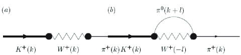
Figure 1: Axial (a) and vector (b) current contribution into $K^{+}\to\pi^{+}$ transition

However, in the case of the vector contribution corresponding to the second diagram in Fig. 1 the radiation version differs from the Lorentz gauge version (54).

In contrast to the Lorentz gauge version (54), two radiation variable diagrams in Fig. 1 in the rest kaon frame $k_{\mu}=(k_{0},0,0,0)$ are reduced to the static interaction contribution

$$i(2\pi)^{4}\delta^{4}(k-p)G_{\rm EW}\Sigma^{R}(k^{2})=\left\langle\pi^{+}\left|-i\int d^{4}xJ_{0}(x)\frac{1}{\triangle-M_{W}^{2}}J_{0}(x)\right|K^{+}\right\rangle$$

with the normal ordering of the pion fields which are at their mass-shell, so that

$$\Sigma^{R}(k^{2})=2k^{2}{F^{2}_{\pi}}\left[1+\frac{M_{W}^{2}}{F^{2}_{\pi}(2\pi)^{3}}\int\frac{d^{3}l}{2E_{\pi}(\vec{l})}\frac{1}{M^{2}_{W}+\vec{l}^{2}}\right]\equiv 2k^{2}{F^{2}_{\pi}}g_{8}.$$ (95)

Here $E_{\pi}(\vec{l})=\sqrt{m^{2}_{\pi}+\vec{l}^{2}}$ is the energy of $\pi$-meson and $g_{8}$ is the parameter of the enhancement of the probability of the axial $K^{+}\to\pi^{+}$ transition. The pion mass-shell justifies the application of the low-energy ChPT [13, 14], where the summation of the chiral series can be considered here as the meson form factors [15, 16, 17] $\int\dfrac{d^{3}l}{2E_{\pi}(\vec{l})}\to$ $\int\dfrac{d^{3}lf^{V}_{K}(-(\vec{l})^{2})f^{V}_{\pi}(-(\vec{l})^{2})}{2E_{\pi}(\vec{l})}$.

Using the covariant perturbation theory [18] developed as the series $\underline{J}_{\mu}^{k}(\gamma\oplus\xi)=\underline{J}_{\mu}^{k}(\xi)+F^{2}_{\pi}\partial_{\mu}\gamma^{k}+\gamma^{i}f_{ijk}\underline{J}_{\mu}^{j}(\xi)+O(\gamma^{2})$ with respect to quantum fields $\gamma$ added to $\xi$ as the product $e^{i\gamma}e^{i\xi}\equiv e^{i(\gamma\oplus\xi)}$, one can see that the normal ordering

$$<0|\gamma^{i}(x)\gamma^{i^{\prime}}(y)|0>=\delta^{ii^{\prime}}N(\vec{z}),~{}~{}~{}~{}N(\vec{z})=\int\frac{d^{3}le^{i\vec{l}\cdot(\vec{z})}}{(2\pi)^{3}2E_{\pi}(\vec{l})},$$

where $\vec{z}=\vec{x}-\vec{y}$, in the product of the currents $\underline{J}_{\mu}^{k}(\gamma\oplus\xi)$ leads to an effective Lagrangian with the rule $\triangle T=1/2$

$$M_{W}^{2}\int d^{3}zg_{8}(z)\frac{e^{-M_{W}|\vec{z}|}}{4\pi|\vec{z}|}[\underline{J}_{\mu}^{j}(x)\underline{J}_{\mu}^{j^{\prime}}(z+x)(f_{ij1}+if_{ij2})(f_{i^{\prime}j^{\prime}4}-if_{i^{\prime}j^{\prime}5})\delta^{ii^{\prime}}+h.c],$$

where $g_{8}(|z|)=[1+\sum\limits_{I\geq 1}c^{I}N^{I}(\vec{z})]$ is series over the multipaticle intermediate states (this sum is known as the Volkov superpropagator [14, 19]). In the limit $M_{W}\to\infty$, in the lowest order with respect to $M_{W}$, the dependence of $g_{8}(|\vec{z}|)$ and the currents on $\vec{z}$ disappears in the integral of the type of

$$M^{2}_{W}\int d^{3}z\dfrac{g_{8}(|\vec{z}|)e^{-M_{W}|\vec{z}|}}{4\pi|\vec{z}|}=\int_{0}^{\infty}drre^{-r}g_{8}({r}/{M_{W}})\simeq g_{8}(0).$$

In the next order, the amplitudes $K^{0}(\bar{K}^{0})\to\pi^{0}$ arise. Finally, we get the effective Lagrangians [20]

$$\mathcal{L}_{(\Delta T=\frac{1}{2})} = \frac{G_{F}}{\sqrt{2}}g_{8}(0)\cos\theta_{C}\sin\theta_{C}\times$$

$$\left[(\underline{J}^{1}_{\mu}+i\underline{J}^{2}_{\mu})(\underline{J}^{4}_{\mu}-i\underline{J}^{5}_{\mu})-\left(\underline{J}^{3}_{\mu}+\frac{1}{\sqrt{3}}\underline{J}^{8}_{\mu}\right)(\underline{J}^{6}_{\mu}-i\underline{J}^{7}_{\mu})+h.c.\right],$$

$$\mathcal{L}_{(\Delta T=\frac{3}{2})}=\frac{G_{F}}{\sqrt{2}}\cos\theta_{C}\sin\theta_{C}\left[\left(\underline{J}^{3}_{\mu}+\frac{1}{\sqrt{3}}\underline{J}^{8}_{\mu}\right)(\underline{J}^{6}_{\mu}-i\underline{J}^{7}_{\mu})+h.c.\right].$$ (97)

This result shows that the enhancement can be explained by static vector interaction that increases the $K^{+}\to\pi^{+}$ transition by a factor of $g_{8}=g_{8}(0)$, and yields a new term describing the $K^{0}\to\pi^{0}$ transition proportional to $g_{8}-1$.

This Lagrangian with the fit parameter $g_{8}=5$ (i.e. $g_{8}\sin\theta_{C}\cos\theta_{C}\simeq 1$) describes the nonleptonic decays in satisfactory agreement with experimental data [14, 20, 21].

Thus, for normal ordering of the weak static interaction in the Hamiltonian SM can explain the rule $\triangle T=1/2$ and universal factor $g_{8}$.

On the other hand, contact character of weak static interaction in the Hamiltonian SM excludes all retarded diagram contributions in the effective Chiral Perturbation Theory considered in [23] that destruct the form factor structure of the kaon radiative decay rates with the amplitude

$$T_{(K^{+}\to\pi^{+}l^{+}l^{-})}=g_{8}t(q^{2})2F^{2}_{\pi}\sin\theta_{C}\cos\theta_{C}\dfrac{G_{F}}{\sqrt{2}}\dfrac{(k_{\mu}+p_{\mu})}{q^{2}}\bar{l}\gamma_{\mu}l\,\,\,$$ (98)

where $q^{2}=(k-p)^{2}$, and

$$t(q^{2})=\dfrac{f^{A}_{K}(q^{2})\!+\!f^{A}_{\pi}(q^{2})}{2}-f^{V}_{\pi}(q^{2})+\Big{[}\!f^{V}_{K}(q^{2})\!-\!f^{V}_{\pi}(q^{2})\!\Big{]}\dfrac{m_{\pi}^{2}}{M_{K}^{2}-m_{\pi}^{2}},$$ (99)

and $f_{K}^{V}\simeq f_{\pi}^{V}(q^{2})=1+M^{-2}_{\rho}q^{2}+...$, $f_{K}^{A}(q^{2})\simeq f_{\pi}^{A}(q^{2})=1+M^{-2}_{a}q^{2}+\ldots$ are form factors determined by the masses of the nearest resonances for meson – gamma – meson vertex.

Therefore, the static interaction mechanism of the enhancement of the $\triangle T=1/2$ transitions predicts [21] that the meson form factor resonance parameters explains the experimental values of rates of the radiation kaon decays $K^{+}\to\pi^{+}e^{+}e^{-}(\mu^{+}\mu^{-})$. Actually, substituting of the PDG data on the resonance masses $M_{\rho}=775.8$ MeV, $1^{+}(1^{--})=I^{G}(J^{PC})$ and meson – gamma – W-boson one $M_{a}=984.7$ MeV, $1^{-}(0^{++})=I^{G}(J^{PC})$ into the decay amplitudes one can obtain decay branching fractions [21]:

$${\rm Br}(K^{+}\to\pi^{+}e^{+}e^{-}) = 2.93\times 10^{-7},~{}~{}[2.88\pm 0.13\times 10^{-7}]_{\rm PDG}$$

$${\rm Br}(K^{+}\to\pi^{+}\mu^{+}\mu^{-}) = 0.73\times 10^{-7},~{}~{}[0.81\pm 0.14\times 10^{-7}]_{\rm PDG}$$ (100)

in satisfactory agreement with the experimental data [24, 25]. Thus, the off-mass-shell kaon-pion transition in the radiation weak kaon decays can be a good probe of the weak static interaction revealed by the radiation propagator (53) of the Hamiltonian presentation of SM.

5 Conclusions

Physical consequences of the Hamiltonian approach to the Standard Model are the weak static interactions, like the Coulomb static interaction is consequence of the Hamiltonian approach in QED. The static interactions can be omitted, if we restrict ourselves by the scattering processes of the elementary particles where static interactions are not important. However, the static poles play crucial role in the mass-shell phenomena of the bound state type, spontaneous symmetry breaking, kaon - pion transition in the weak decays, etc. Static interactions follow from the spectrality principle that means existence of a vacuum defined as a state with the minimal energy. We discussed physical effects testifying about the static interactions omitted by the accepted version of SM.

One of these effects is revealed by the loop meson diagrams in the low energy weak static interaction. These diagrams lead to the enhancement coefficient $g_{8}$ in weak kaon decays and the rule $\triangle T=\frac{1}{2}$. The loop pion diagrams in the Chiral Perturbation Theory [14] in the framework of the Hamiltonian approach with the weak static interaction lead to definite relation of the vector form factor with the differential radiation kaon decay rates in agreement with the present day PDG data [21], in the contrast to the acceptable renormalization group analysis based on the Lorentz gauge formulation omitting weak static interaction [23], where loop pion diagrams destroy the above mentioned relation of the vector form factor with the differential radiation kaon decay rates. Therefore, the radiation kaon decays can be a good probe of the weak static interaction.

The Hamiltonian approach to the Standard Model and its operator fundamental formulation lead to a dynamic version of spontaneous symmetry breaking and the Schwinger – Dyson type equation provoking the sum-rule of masses of vector and spinor fields that predicts the mass of Higgs particle $\simeq 310\pm 10$ GeV.

References

• [1] P.A.M. Dirac, Proc. Roy. Soc., A 114, 243 (1927); Can. J. Phys., 33, 650 (1955).
• [2] W. Heisenberg, W. Pauli, Z. Phys. 56, 1 (1929); Z.Phys. 59, 166 (1930).
• [3] J. Schwinger, Phys. Rev., 127, 324 (1962).
• [4] I.V. Polubarinov, Physics of Particles and Nuclei, 34, 377 (2003).
• [5] V.N. Pervushin, Physics of Particles and Nuclei, 34, 348 (2003).
• [6] H.-P. Pavel, V.N. Pervushin, Int. J. Mod. Phys. A 14, 2885 (1999).
• [7] L.D. Faddeev, T. M. F., 1, 3 (1969).
• [8] L.D. Faddeev, V.N. Popov, Phys. Lett. B 25, 29 (1967).
• [9] D. Bardin, G. Passarino, The standard model in the making: precision study of the electroweak interactions, Clarendon, Oxford, 1999.
• [10] S.A. Gogilidze, V.N. Pervushin, and A.M. Khvedelidze, Physics of Particle and Nuclei, 30, 66 (1999).
• [11] C.N. Yang, R.L. Mills, Phys.Rev. 96 191 (1954).
• [12] S.L. Glashow, Nucl.Phys. 22 579 (1961);
Weinberg S. Phys.Rev.Lett, 19 1264 (1967);
A. Salam, The standard model. Almqvist and Wikdells, Stockholm 1969. In ”Elementary Particle Theory”, ed. N. Svartholm, p.367.
• [13] M. Volkov, V. Pervushin, Phys. Lett. B51, 356 (1974).
• [14] M. K. Volkov and V. N. Pervushin, Usp. Fiz. Nauk 120, 363 (1976).
M. K. Volkov and V. N. Pervushin, “Essentially Nonlinear Field Theory, Dynamical Symmetry and Pion Physics”, Atomizdat, Moscow, ed. D.I. Blokhintsev, 1979 (in Russian).
• [15] A.A. Bel’kov, Yu. L. Kalinovsky, V. N. Pervushin, JINR-P2-85-107 (1985).
A.A. Bel’kov et al., Yad. Fis. 44, 690 (1986).
• [16] G. Ecker et al., Nucl. Phys. B291, 692 (1987); G. Ecker, Prog. Part. Nucl. Phys. 36, 71 (1996); hep-ph/9511412.
• [17] A.A. Bel’kov et al., Phys. Part. Nucl. 26, 239 (1995).
A.A. Bel’kov, Phys. Part. Nucl. 36, 509 (2005).
• [18] V.N. Pervushin, Theor. Math. Phys. 27, 330 (1977); D.I. Kazakov, V.N. Pervushin, S.V. Pushkin, J. Phys. A. Math. Gen. 11, 2093 (1978).
• [19] M.K. Volkov, Ann. Phys. (N. Y.) 49, 202 (1968); C.J. Isham, Abdus Salam, and J. Strathdee, Phys. Rev. D 3, 1805 (1971).
• [20] Yu.L. Kalinovsky, V.N. Pervushin, Sov. J. Nucl. Phys., 29, 225 (1979).
• [21] A.Z. Dubnickova, S. Dubnicka, E. Goudzovski, V.N. Pervushin, M. Secansky, Talk at the 5th NA48 Mini-Workshop on kaon physics (CERN, December 12, 2006) hep-ph/0611175; be published in Particles and Nuclei, Letters Vol. 4, (2007)
• [22] Yu. L. Kalinovsky, V. N. Pervushin, Sov. J. Nucl. Phys., 29, 475 (1979).
• [23] G. D’Ambrosio et al., JHEP 9808, 4 (1998).
• [24] R. Appel et al., Phys. Rev. Lett. 83, 4482 (1999).
• [25] Journal of Physics G: Nuclear and Particle Physics Vol 33. Review of Particle Physics, 2006