LPTENS–06/55

LTH–715

hep-th/0611251

June 2006

Spinor–Vector Duality
in
fermionic $Z_{2}\times Z_{2}$ heterotic orbifold models Alon E. Faraggi¹, Costas Kounnas² and John Rizos^3
1 Dept. of Mathematical Sciences, University of Liverpool, Liverpool L69 7ZL, UK
² Lab. Physique Théorique, Ecole Normale Supérieure, F–75231 Paris 05, France
³ Department of Physics, University of Ioannina, GR45110 Ioannina, Greece

We continue the classification of the fermionic $Z_{2}\times Z_{2}$ heterotic string vacua with symmetric internal shifts. The space of models is spanned by working with a fixed set of boundary condition basis vectors and by varying the sets of independent Generalized GSO (GGSO) projection coefficients (discrete torsion). This includes the Calabi–Yau like compactifications with (2,2) world–sheet superconformal symmetry, as well as more general vacua with only (2,0) superconformal symmetry. In contrast to our earlier classification that utilized a montecarlo technique to generate random sets of GGSO phases, in this paper we present the results of a complete classification of the subclass of the models in which the four dimensional gauge group arises solely from the null sector. In line with the results of the statistical classification we find a bell shaped distribution that peaks at vanishing net number of generations and with $\sim$15% of the models having three net chiral families. The complete classification reveals a novel spinor–vector duality symmetry over the entire space of vacua. The $S_{t}\leftrightarrow V$ duality interchanges the spinor plus anti–spinor representations with vector representations. We present the data that demonstrates the spinor–vector duality. We illustrate the existence of a duality map in a concrete example. We provide a general algebraic proof for the existence of the $S_{t}\leftrightarrow V$ duality map. We discuss the case of self–dual solutions with an equal number of vectors and spinors, in the presence and absence of $E_{6}$ gauge symmetry, and presents a couple of concrete examples of self–dual models without $E_{6}$ symmetry.

1 Introduction

In the framework of the free fermionic construction [1, 2] of the heterotic string many three generation realistic string models can be constructed in four dimensions with the correct quantum numbers under the Standard Model gauge group [3]. In the orbifold language the free fermionic models corresponds to a either symmetric or asymmetric, or freely acting, orbifolds. In particular, a subclass of the free fermionic vacua correspond to symmetric $Z_{2}\times Z_{2}$ orbifold compactifications at enhanced symmetry points in the toroidal moduli space [4, 5]. In this class of orbifold models the chiral matter spectrum arises from twisted sectors and thus does not depend on the moduli. This allows the development of a complete classification of $Z_{2}\times Z_{2}$ symmetric orbifolds. The free fermionic construction provides the techniques which facilitate developing a computerized classification algorithm for the twisted matter chiral spectrum. Thus, the free fermionic formalism provides powerful tools for the systematic classification of symmetric $Z_{2}\times Z_{2}$ perturbative string orbifold models.

For type II string $N=2$ supersymmetric vacua the general free fermionic classification techniques were developed in ref. [6]. The method was extended in refs. [7, 8, 9] for the classification of heterotic $Z_{2}\times Z_{2}$ orbifolds. In this class of models the six dimensional internal manifold contains three twisted sectors. In the heterotic string each of these sectors may, or may not, a priori (prior to application of the Generalized GSO (GGSO) projections), give rise to spinorial representations. Generically we may classify the models as $S^{3}$, $S^{2}V$, $SV^{2}$ and $V^{3}$ classes of models, with spinorial representations arising from three, two, one or none of the twisted sectors, respectively. A priori it may be thought that the classification of the different classes of models would require different sets of basis vectors. However, In ref. [9] we demonstrated that the entire sets of $S^{3},~{}S^{2}V,~{}SV^{2}$ and $V^{3}$ classes of models are produced by working with the single basis set of ref. [7], according to specific choices of the one–loop Generalized GSO (GGSO) projection coefficients (discrete torsions). This fact is of basic importance since it enables a systematic analysis of all the models and the representation of their main features, like the number of spinorial, anti–spinorial and vectorial representations, in algebraic formulas.

The classification methodology that we developed allows us to scan a range of over $10^{16}$ models, and therefore obtain vital insight into the properties of the entire space of symmetric $Z_{2}\times Z_{2}$ orbifold vacua. The space of vacua in this class of models arises from a set of independent binary GGSO projection coefficients $c{b_{i}\atopwithdelims[ ]b_{j}}$, which correspond a matrix with elements taking values $\pm 1$. The independent elements of this matric correspond to the upper block of this matrix. All other elements are fixed by modular invariance and factorization of the partition function [1]. The classification basis of ref. [7] contains 12 vectors. Therefore, the number of independent GGSO projection coefficients is 66. Requiring $N=1$ space–time supersymmetry reduces the number of independent phases to 55. Hence, prior to imposing further constraints the space of models that we scan contains $2^{55}$ different vacua. This space of models is still too large for a complete computerized classification. Therefore, in ref. [9] we resorted to a montecarlo technique to generate random choices of phases. Our computer method checked that only new models are recounted and in this manner we were able to explore a set of some $10^{10}$ distinct vacua.

The analysis in ref. [9] revealed a bell shape distribution that peaks at vanishing net number of chiral families, with about 15% of the models having three net chiral families. The statistical analysis also revealed an additional symmetry in the distribution of $Z_{2}\times Z_{2}$ string vacua under exchange of vectorial, and spinorial plus anti–spinorial, representations of $SO(10)$. This symmetry is akin to mirror symmetry which exchanges spinorial with anti–spinorial representations. The symmetry is observed by noting that the same number of models are generated under the exchange.

In this paper we continue the study of the classification with particular focus on the exploration of the new symmetry under the exchange of spinorial and vectorial representations. In particular, for this purpose we modify the method of analysis. Rather than using montecarlo generation of random sets of GGSO phases sets, we perform a complete classification of a restricted class of models. The restricted class is selected by imposing that the only space-time vector bosons that arise in the models are those that are obtained from the untwisted Neveu–Schwarz sector. Vector bosons that may arise from other sectors are projected out by the specific choice of GGSO projection coefficients. This is achieved by restricting the choices of GGSO projection coefficients and hence restricting the space of models, and enables a complete computerized classification of the subclass of vacua. This restricts the four dimensional gauge group in these models to be $SO(10)\times U(1)^{3}\times SO(8)\times SO(8)$, and eliminates enhancements $SO(10)\times U(1)\rightarrow E_{6}$ as well as all enhancements of the $SO(8)\times SO(8)$.

The complete classification of this restricted class again reveals the symmetry under exchange of the total number of spinors plus anti–spinors with the number of vectors in the space of string vacua. Furthermore, we note that the symmetry operates on each of the three twisted sectors of the $Z_{2}\times Z_{2}$ orbifold. We note that the symmetry under this exchange is evident when the $SO(10)$ symmetry is enhanced to $E_{6}$, in which case $\#(16+{\overline{1}6})=\#(10)$. We demonstrate that the symmetry persists also when there is no enhancement to $E_{6}$. We further show the existence of self–dual vacua in which $\#(16+{\overline{1}6})=\#(10)$, but in which the $SO(10)$ symmetry is not enhanced to $E_{6}$.

Our paper is organised as follows: in section 2 we review the method of classification for completeness. In section 3 we elaborate on the counting method of $SO(10)$ spinorial and vectorial representations. In section 4 we discuss the conditions imposed on the four dimensional gauge group and their implementation in the classification method. In section 5 we discuss the results of the classification in comparison to the statistical classification of ref. [9]. In section 6 we discuss the spinor–vector duality. In section 7 we provide an analytic proof of the spinor–vector duality. In section 8 we demonstrate the existence of vacua that are self–dual under the spinor–vector interchange, but in which the $SO(10)$ symmetry is not enhanced to $E_{6}$. Section 9 concludes the paper.

2 Review of the classification method

In the free fermionic formulation the 4-dimensional heterotic string, in the light-cone gauge, is described by $20$ left–moving and $44$ right–moving two dimensional real fermions [1, 2]. A large number of models can be constructed by choosing different phases picked up by fermions ($f_{A},A=1,\dots,44$) when transported along the torus non-contractible loops. Each model corresponds to a particular choice of fermion phases consistent with modular invariance that can be generated by a set of basis vectors $v_{i},i=1,\dots,n$,

$$v_{i}=\left\{\alpha_{i}(f_{1}),\alpha_{i}(f_{2}),\alpha_{i}(f_{3}))\dots\right\}$$

describing the transformation properties of each fermion

$$f_{A}\to-e^{i\pi\alpha_{i}(f_{A})}\ f_{A},\ ,A=1,\dots,44~{}.$$ (2.1)

The basis vectors span a space $\Xi$ which consists of $2^{N}$ sectors that give rise to the string spectrum. Each sector is given by

$$\xi=\sum N_{i}v_{i},\ \ N_{i}=0,1$$ (2.2)

The spectrum is truncated by a GGSO projection whose action on a string state $|S>$ is

$$e^{i\pi v_{i}\cdot F_{S}}|S>=\delta_{S}\ c{S\atopwithdelims[ ]v_{i}}|S>,$$ (2.3)

where $F_{S}$ is the fermion number operator and $\delta_{S}=\pm 1$ is the spacetime spin statistics index. Different sets of projection coefficients $c{S\atopwithdelims[ ]v_{i}}=\pm 1$ consistent with modular invariance give rise to different models. Summarizing: a model can be defined uniquely by a set of basis vectors $v_{i},i=1,\dots,n$ and a set of $2^{N(N-1)/2}$ independent projections coefficients $c{v_{i}\atopwithdelims[ ]v_{j}},i>j$.

The two dimensional free fermions in the light-cone gauge (in the usual notation [1, 2, 3]) are: $\psi^{\mu},\chi^{i},y^{i},\omega^{i},i=1,\dots,6$ (real left-moving fermions) and $\bar{y}^{i},\bar{\omega}^{i},i=1,\dots,6$ (real right-moving fermions), ${\bar{\psi}}^{A},A=1,\dots,5$, $\bar{\eta}^{B},B=1,2,3$, $\bar{\phi}^{\alpha},\alpha=1,\ldots,8$ (complex right-moving fermions). The class of models under investigation, is generated by a set $V$ of 12 basis vectors

$$V=\{v_{1},v_{2},\dots,v_{12}\},$$

where

$$v_{1}=1 = \{\psi^{\mu},\ \chi^{1,\dots,6},y^{1,\dots,6},\omega^{1,\dots,6}|$$

$$~{}~{}~{}\bar{y}^{1,\dots,6},\bar{\omega}^{1,\dots,6},\bar{\eta}^{1,2,3},\bar{\psi}^{1,\dots,5},\bar{\phi}^{1,\dots,8}\},$$

$$v_{2}=S = \{\psi^{\mu},\chi^{1,\dots,6}\},$$

$$v_{2+i}=e_{i} = \{y^{i},\omega^{i}|\bar{y}^{i},\bar{\omega}^{i}\},\ i=1,\dots,6,$$

$$v_{9}=b_{1} = \{\chi^{34},\chi^{56},y^{34},y^{56}|\bar{y}^{34},\bar{y}^{56},\bar{\eta}^{1},\bar{\psi}^{1,\dots,5}\},$$ (2.4)

$$v_{10}=b_{2} = \{\chi^{12},\chi^{56},y^{12},y^{56}|\bar{y}^{12},\bar{y}^{56},\bar{\eta}^{2},\bar{\psi}^{1,\dots,5}\},$$

$$v_{11}=z_{1} = \{\bar{\phi}^{1,\dots,4}\},$$

$$v_{12}=z_{2} = \{\bar{\phi}^{5,\dots,8}\}.$$

The vectors $1,S$ generate an $N=4$ supersymmetric model, with $SO(44)$ gauge symmetry. The vectors $e_{i},i=1,\dots,6$ give rise to all possible symmetric shifts of the six internal fermionized coordinates ($\partial X^{i}=y^{i}\omega^{i},{\bar{\partial}}X^{i}=\bar{y}^{i}\bar{\omega}^{i}$). Their addition breaks the $SO(44)$ gauge group, but preserves $N=4$ supersymmetry. The vectors $b_{1}$ and $b_{2}$ defines the $Z_{2}\times Z_{2}$ orbifold twists, which breaks $N=4$ to $N=1$ supersymmetry, and defines the $SO(10)$ gauge symmetry. The $z_{1}$ and $z_{2}$ basis vectors give rise to the $SO(8)\times SO(8)$ gauge group. It is important to note here that the above choice of $V$ is the most general set of basis vectors, compatible with a $SO(10)$ Kac–Moody level one algebra.

Without loss of generality we can fix some of the associated GGSO projection coefficients

$$c{1\atopwithdelims[ ]1}=c{1\atopwithdelims[ ]S}=c{S\atopwithdelims[ ]S}=c{S\atopwithdelims[ ]e_{i}}=c{S\atopwithdelims[ ]b_{A}}=-c{b_{2}\atopwithdelims[ ]S}=c{S\atopwithdelims[ ]z_{n}}=-1,~{}$$

leaving 55 independent coefficients,

$$c{e_{i}\atopwithdelims[ ]e_{j}},i\geq j,\ \ c{b_{1}\atopwithdelims[ ]b_{2}},\ \ c{z_{1}\atopwithdelims[ ]z_{2}},$$

$$c{e_{i}\atopwithdelims[ ]z_{n}},c{e_{i}\atopwithdelims[ ]b_{A}},c{b_{A}\atopwithdelims[ ]z_{n}},\ \ i,j=1,\dots 6\,\ ,\ A,B,m,n=1,2,$$

since all of the remaining projection coefficients are determined by modular invariance [1, 2]. Each of the 55 independent coefficients can take two discrete values $\pm 1$ and thus a simple counting gives $2^{55}$ (that is approximately $10^{16.6}$) distinct models in the class of superstring vacua under consideration.

The vector bosons from the untwisted sector generate an $SO(10)\times{U(1)}^{3}\times{SO(8)}^{2}$gauge symmetry. Depending on the choices of the projection coefficients, extra gauge bosons may arise from

$$x=1+S+\sum_{i=1}^{6}e_{i}+z_{1}+z_{2}=\{{\bar{\eta}^{123},\bar{\psi}^{12345}}\}~{},$$ (2.5)

which enhances the gauge group $SO(10)\times{U(1)}\to E_{6}$. Additional gauge bosons can arise as well from the sectors $z_{1},z_{2}$ and $z_{1}+z_{2}$ and enhance the hidden gauge group ${SO(8)}^{2}\to SO(16)$ or even ${SO(8)}^{2}\to E_{8}$. Indeed, as was shown in ref. [7], for particular choices of the projection coefficients a variety of gauge groups is obtained. The classification in this paper is restricted to the case in which all the gauge bosons from the sectors $x$, $z_{1}$ ,$z_{2}$ and $z_{1}+z_{2}$ are projected out. Hence, in the entire space of vacua the four dimensional gauge group is $SO(10)\times{U(1)}^{3}\times{SO(8)}^{2}.$

The matter spectrum from the untwisted sector is common to all models and consists of six vectors of $SO(10)$ and 12 states that singlets under the non-Abelian gauge groups. The chiral spinorial representations arise necessarily from the following 48 twisted sectors

$$B_{\ell_{3}^{1}\ell_{4}^{1}\ell_{5}^{1}\ell_{6}^{1}}^{1} = S+b_{1}+\ell_{3}^{1}e_{3}+\ell_{4}^{1}e_{4}+\ell_{5}^{1}e_{5}+\ell_{6}^{1}e_{6}$$

$$B_{\ell_{1}^{2}\ell_{2}^{2}\ell_{5}^{2}\ell_{6}^{2}}^{2} = S+b_{2}+\ell_{1}^{2}e_{1}+\ell_{2}^{2}e_{2}+\ell_{5}^{2}e_{5}+\ell_{6}^{2}e_{6}$$ (2.6)

$$B_{\ell_{1}^{3}\ell_{2}^{3}\ell_{3}^{3}\ell_{4}^{3}}^{3} = S+b_{3}+\ell_{1}^{3}e_{1}+\ell_{2}^{3}e_{2}+\ell_{3}^{3}e_{3}+\ell_{4}^{3}e_{4}$$

where $\ell_{i}^{j}=0,1$; $b_{3}=b_{1}+b_{2}+x=1+S+b_{1}+b_{2}+\sum_{i=1}^{6}e_{i}+\sum_{n=1}^{2}z_{n}$ and $x$ is given in eq. (2.5).

The states that arise from the sectors in (2.6) are spinorials of $SO(10)$ and one can obtain at most one spinorial ($\bf 16$ or $\bf{\overline{{16}}}$) per sector and thus totally 48 spinorials. The states in the vector representation of $SO(10)$ arise necessarily from the $x$–mapped twisted sectors $B_{\ell_{3}^{i}\ell_{4}^{i}\ell_{5}^{i}\ell_{6}^{i}}^{i}+x$ , $(i=1,2,3)$, accompanied always by six singlets under $SO(10)\times SO(8)\times SO(8)$.

The string vacua generically may contain additional hidden matter states that transform under the hidden sector gauge group. These arise generically from the sectors $B_{\ell_{3}^{i}\ell_{4}^{i}\ell_{5}^{i}\ell_{6}^{i}}^{i}+x$ , $B_{\ell_{3}^{i}\ell_{4}^{i}\ell_{5}^{i}\ell_{6}^{i}}^{i}+x+z_{1}$ , and $B_{\ell_{3}^{i}\ell_{4}^{i}\ell_{5}^{i}\ell_{6}^{i}}^{i}+x+z_{2}$ , where $(i=1,2,3)$. The hidden sector matter states appear in general in vector representations, and may be chiral with respect to the unbroken $U(1)$ symmetries, defined by the ${\bar{\eta}}_{1}$, ${\bar{\eta}}_{2}$ and ${\bar{\eta}}_{3}$ world–sheet fermions. Our analysis here focuses on the observable sector states and neglects the hidden sector matter states. An investigation that includes the hidden matter states is of interest, in particular in regard to the modular properties of this space of vacua, but their inclusion is left for future work.

This construction therefore separates the fixed points of the $Z_{2}\times Z_{2}$ orbifold into different sectors. This enables the analysis of the GGSO projection on the spectrum from each individual fixed point separately. Hence, depending on the choice of the GGSO projection coefficients we can distinguish several possibilities for the spectrum from each individual fixed point. For example, in the case of enhancement of the $SO(10)$ symmetry to $E_{6}$ each individual fixed point gives rise to spinorial, as well as vectorial representation of $SO(10)$, which are embedded in the $27$ representation of $E_{6}$. When $E_{6}$ is broken each fixed point typically will give rise to either spinorial or vectorial representation of $E_{6}$. However, there exist also rare situations, depending on the choice of GGSO phases, where a fixed point can yield a spinorial as well as vectorial representation of $SO(10)$ without enhancement. The crucial point, however, is that the GGSO projections can be written as simple algebraic conditions, and hence the classification is amenable to a computerized analysis.

3 Counting the twisted matter spectrum

The counting of spinorials proceeds as follows. For each $SO(10)$ spinorial from a twisted sector $B^{i}_{pqrs}$ defined in (2.6) we can write down the associated projector $P^{i}_{pqrs}=0,1$, in terms of the GGSO projection coefficients. The explicit expressions for the 48 projectors are

$$P_{p^{1}q^{1}r^{1}s^{1}}^{(1)} = \frac{1}{4}\,\left(1-c{e_{1}\atopwithdelims[ ]B_{p^{1}q^{1}r^{1}s^{1}}^{(1)}}\right)\,\cdot\left(1-c{e_{2}\atopwithdelims[ ]B_{p^{1}q^{1}r^{1}s^{1}}^{(1)}}\right)\,$$

$$\cdot\frac{1}{4}\left(1-c{z_{1}\atopwithdelims[ ]B_{p^{1}q^{1}r^{1}s^{1}}^{(1)}}\right)\,\cdot\left(1-c{z_{2}\atopwithdelims[ ]B_{p^{1}q^{1}r^{1}s^{1}}^{(1)}}\right)$$

$$P_{p^{2}q^{2}r^{2}s^{2}}^{(2)} = \frac{1}{4}\,\left(1-c{e_{3}\atopwithdelims[ ]B_{p^{2}q^{2}r^{2}s^{2}}^{(2)}}\right)\,\cdot\left(1-c{e_{4}\atopwithdelims[ ]B_{p^{2}q^{2}r^{2}s^{2}}^{(2)}}\right)\,$$ (3.1)

$$\cdot\frac{1}{4}\,\left(1-c{z_{1}\atopwithdelims[ ]B_{p^{2}q^{2}r^{2}s^{2}}^{(2)}}\right)\,\cdot\left(1-c{z_{2}\atopwithdelims[ ]B_{p^{2}q^{2}r^{2}s^{2}}^{(2)}}\right)$$

$$P_{p^{3}q^{3}r^{3}s^{3}}^{(3)} = \frac{1}{4}\,\left(1-c{e_{5}\atopwithdelims[ ]B_{p^{3}q^{3}r^{3}s^{3}}^{(3)}}\right)\,\cdot\left(1-c{e_{6}\atopwithdelims[ ]B_{p^{3}q^{3}r^{3}s^{3}}^{(3)}}\right)\,$$

$$\cdot\frac{1}{4}\,\left(1-c{z_{1}\atopwithdelims[ ]B_{p^{3}q^{3}r^{3}s^{3}}^{(3)}}\right)\,\cdot\left(1-c{z_{2}\atopwithdelims[ ]B_{p^{3}q^{3}r^{3}s^{3}}^{(3)}}\right)~{}.$$

When $P^{i}_{pqrs}=1$ there is a surviving spinorial (${\bf 16}$ or ${\bf\overline{16}}\,$). For the surviving spinorial ($P^{i}_{pqrs}=1$) the chirality (${\bf 16}$ or ${\bf\overline{16}}\,$) is determined from the associated chirality coefficient $X^{i}_{pqrs}=\pm 1$, where

$$X_{p^{1}q^{1}r^{1}s^{1}}^{(1)} = c{S+b_{2}+(1-r^{1})e_{5}+(1-s^{1})e_{6}\atopwithdelims[ ]B_{p^{1}q^{1}r^{1}s^{1}}^{(1)}}$$

$$X_{p^{2}q^{2}r^{2}s^{2}}^{(2)} = c{S+b_{1}+(1-r^{2})e_{5}+(1-s^{2})e_{6}\atopwithdelims[ ]B_{p^{2}q^{2}r^{2}s^{2}}^{(2)}}$$ (3.2)

$$X_{p^{3}q^{3}r^{3}s^{3}}^{(3)} = c{S+b_{1}+(1-r^{3})e_{3}+(1-s^{3})e_{4}\atopwithdelims[ ]B_{p^{3}q^{3}r^{3}s^{3}}^{(3)}}$$

$$= c{S+b_{2}+(1-p^{3})e_{1}+(1-q^{3})e_{2}\atopwithdelims[ ]B_{p^{3}q^{3}r^{3}s^{3}}^{(3)}}~{}.$$

These formulas are dictated by the vector intersections

$$S+b_{2}+(1-r^{1})e_{5}+(1-s^{1})e_{6}\cap B_{p^{1}q^{1}r^{1}s^{1}}^{(1)} =$$

$$S+b_{1}+(1-r^{2})e_{5}+(1-s^{2})e_{6}\cap B_{p^{2}q^{2}r^{2}s^{2}}^{(2)} =$$

$$S+b_{1}+(1-r^{3})e_{3}+(1-s^{3})e_{4}\cap B_{p^{3}q^{3}r^{3}s^{3}}^{(3)} =$$

$$S+b_{2}+(1-p^{3})e_{1}+(1-q^{3})e_{2}\cap B_{p^{3}q^{3}r^{3}s^{3}}^{(3)} = \{\bar{\psi}^{12345}\}~{}.$$

Using the above results, we can easily calculate the number of spinorials/antispinorial per sector

$$S_{\pm}^{(i)} = \sum_{pqrs}\frac{1\pm X^{(i)}_{p^{i}q^{i}r^{i}s^{i}}}{2}P_{p^{i}q^{i}r^{i}s^{i}}^{(i)}\ ,\ i=1,2,3$$ (3.3)

The counting of $SO(10)$ vectorials can proceed in a similar way. For each vectorial generating sector $(B_{pqrs})^{i}+x$ the associated projector $(\tilde{P}_{pqrs})^{i}$ is obtained from (3.1) using the replacement $(B_{pqrs})^{i}\to(B_{pqrs})^{i}+x$. Since there is no chirality in this case the number of vectorials per sector is just the sum of the projectors

$$V^{(i)}=\sum_{pqrs}(\tilde{P}_{pqrs})^{(i)}$$ (3.4)

The total number of vectors ($V$), the total number of spinors plus anti–spinors ($S_{t}$), and the net number of spinors minus anti–spinors ($S_{c}$) are given by

$$V=\sum_{i=1}^{3}V^{(i)},$$ (3.5)

$$S_{t}=\sum_{i=1}^{3}S_{+}^{(i)}+S_{-}^{(i)}$$ (3.6)

and

$$S_{c}=\sum_{i=1}^{3}S_{+}^{(i)}-S_{-}^{(i)},$$ (3.7)

respectively.

The mixed projection coefficients entering the above formulas can be decomposed in terms of the independent phases $c{v_{i}\atopwithdelims[ ]v_{j}},i>j$. After some algebra we come to the conclusion that for the counting of the spinorial/antispinorial and vectorial $SO(10)$ states the phases $c{e_{i}\atopwithdelims[ ]e_{i}},i=1,\dots,6$, $c{z_{A}\atopwithdelims[ ]z_{A}},A=1,\dots,2$, $c{b_{I}\atopwithdelims[ ]b_{I}},I=1,\dots,2$ as well as $c{e_{3}\atopwithdelims[ ]b_{1}},c{e_{4}\atopwithdelims[ ]b_{1}},c{e_{1}\atopwithdelims[ ]b_{2}},c{e_{2}\atopwithdelims[ ]b_{2}}$ are not relevant. Moreover the phase $c{b_{1}\atopwithdelims[ ]b_{2}}$ is related to the total chirality flip. This leaves a set of 40 independent phases which is still too large for a manageable computer analysis.

To reduce the number of independent GGSO phases further, we restrict the classification to the space of models in which the four dimensional gauge group arises solely from the untwisted sector. This fixes some additional phases, as we detail below. With respect to this subclass of four dimensional solutions the classification is complete.

We can get more information regarding the possible spinorial and vectorial multiplicities per plane by rewriting the projectors (3.1) in the form of a system of equations. Introducing the notation

$$c{a_{i}\atopwithdelims[ ]a_{j}}=e^{i\pi\left(a_{i}\left|a_{j}\right.\right)}\,\ ,\ \left(a_{i}\left|a_{j}\right.\right)=0,1$$ (3.8)

with the properties

$$\left(a_{i}\left|a_{j}+a_{k}\right.\right) = \left(a_{i}\left|a_{j}\right.\right)+\left(a_{i}\left|a_{k}\right.\right)\ ,\forall\ a_{i}:\{\psi^{\mu}\}\cap a_{i}=\O$$ (3.9)

$$\left(a_{i}\left|a_{j}\right.\right) = \left(a_{j}\left|a_{i}\right.\right)\ ,\forall\ a_{i},a_{j}:a_{i}\cdot a_{j}=0\ {\rm mod}\ 4$$ (3.10)

where $\#(a_{i}\cdot a_{j})\equiv\#\left[a_{i}\cup a_{j}-a_{i}\cap a_{j}\right]$. The projectors can be written as system of equations (one per plane)

$$\Delta^{(I)}\,U_{16}^{(I)}=Y_{16}^{(I)}\ ,\ \Delta^{(I)}\,U_{10}^{(I)}=Y_{10}^{(I)}\ ,\ I=1,2,3$$ (3.11)

where the unknowns are the fixed point labels

$$U_{16}^{(I)}=\left[\begin{array}[]{c}p_{16}^{I}\\ q_{16}^{I}\\ r_{16}^{I}\\ s_{16}^{I}\end{array}\right]\ ,\ U_{10}^{(I)}=\left[\begin{array}[]{c}p_{10}^{I}\\ q_{10}^{I}\\ r_{10}^{I}\\ s_{10}^{I}\end{array}\right]$$ (3.20)

and

$$\Delta^{(1)} = \left[\begin{array}[]{cccc}\left(e_{1}\left|e_{3}\right.\right)&\left(e_{1}\left|e_{4}\right.\right)&\left(e_{1}\left|e_{5}\right.\right)&\left(e_{1}\left|e_{6}\right.\right)\\ \left(e_{2}\left|e_{3}\right.\right)&\left(e_{2}\left|e_{4}\right.\right)&\left(e_{2}\left|e_{5}\right.\right)&\left(e_{2}\left|e_{6}\right.\right)\\ \left(z_{1}\left|e_{3}\right.\right)&\left(z_{1}\left|e_{4}\right.\right)&\left(z_{1}\left|e_{5}\right.\right)&\left(z_{1}\left|e_{6}\right.\right)\\ \left(z_{2}\left|e_{3}\right.\right)&\left(z_{2}\left|e_{4}\right.\right)&\left(z_{2}\left|e_{5}\right.\right)&\left(z_{2}\left|e_{6}\right.\right)\end{array}\right]$$ (3.25)

$$\Delta^{(2)} = \left[\begin{array}[]{cccc}\left(e_{3}\left|e_{1}\right.\right)&\left(e_{3}\left|e_{2}\right.\right)&\left(e_{3}\left|e_{5}\right.\right)&\left(e_{3}\left|e_{6}\right.\right)\\ \left(e_{4}\left|e_{1}\right.\right)&\left(e_{4}\left|e_{2}\right.\right)&\left(e_{4}\left|e_{5}\right.\right)&\left(e_{4}\left|e_{6}\right.\right)\\ \left(z_{1}\left|e_{1}\right.\right)&\left(z_{1}\left|e_{2}\right.\right)&\left(z_{1}\left|e_{5}\right.\right)&\left(z_{1}\left|e_{6}\right.\right)\\ \left(z_{2}\left|e_{1}\right.\right)&\left(z_{2}\left|e_{2}\right.\right)&\left(z_{2}\left|e_{5}\right.\right)&\left(z_{2}\left|e_{6}\right.\right)\end{array}\right]$$ (3.30)

$$\Delta^{(3)} = \left[\begin{array}[]{cccc}\left(e_{5}\left|e_{1}\right.\right)&\left(e_{5}\left|e_{2}\right.\right)&\left(e_{5}\left|e_{3}\right.\right)&\left(e_{5}\left|e_{4}\right.\right)\\ \left(e_{6}\left|e_{1}\right.\right)&\left(e_{6}\left|e_{2}\right.\right)&\left(e_{6}\left|e_{3}\right.\right)&\left(e_{6}\left|e_{4}\right.\right)\\ \left(z_{1}\left|e_{1}\right.\right)&\left(z_{1}\left|e_{2}\right.\right)&\left(z_{1}\left|e_{3}\right.\right)&\left(z_{1}\left|e_{4}\right.\right)\\ \left(z_{2}\left|e_{1}\right.\right)&\left(z_{2}\left|e_{2}\right.\right)&\left(z_{2}\left|e_{3}\right.\right)&\left(z_{2}\left|e_{4}\right.\right)\end{array}\right]$$ (3.35)

$$Y_{16}^{(1)}=\left[\begin{array}[]{c}\left(e_{1}\left|b_{1}\right.\right)\\ \left(e_{2}\left|b_{1}\right.\right)\\ \left(z_{1}\left|b_{1}\right.\right)\\ \left(z_{2}\left|b_{1}\right.\right)\end{array}\right]\ \ \ ,\ Y_{16}^{(2)}=\left[\begin{array}[]{c}\left(e_{3}\left|b_{2}\right.\right)\\ \left(e_{4}\left|b_{2}\right.\right)\\ \left(z_{1}\left|b_{2}\right.\right)\\ \left(z_{2}\left|b_{2}\right.\right)\end{array}\right]\ ,\ Y_{16}^{(3)}=\left[\begin{array}[]{c}\left(e_{5}\left|b_{3}\right.\right)\\ \left(e_{6}\left|b_{3}\right.\right)\\ \left(z_{1}\left|b_{3}\right.\right)\\ \left(z_{2}\left|b_{3}\right.\right)\end{array}\right]$$ (3.48)

$$Y_{10}^{(1)}=\left[\begin{array}[]{c}\left(e_{1}\left|b_{1}+x\right.\right)\\ \left(e_{2}\left|b_{1}+x\right.\right)\\ \left(z_{1}\left|b_{1}+x\right.\right)\\ \left(z_{2}\left|b_{1}+x\right.\right)\end{array}\right]\ \ \ ,\ Y_{10}^{(2)}=\left[\begin{array}[]{c}\left(e_{3}\left|b_{2}+x\right.\right)\\ \left(e_{4}\left|b_{2}+x\right.\right)\\ \left(z_{1}\left|b_{2}+x\right.\right)\\ \left(z_{2}\left|b_{2}+x\right.\right)\end{array}\right]\ ,\ Y_{10}^{(3)}=\left[\begin{array}[]{c}\left(e_{5}\left|b_{3}+x\right.\right)\\ \left(e_{6}\left|b_{3}+x\right.\right)\\ \left(z_{1}\left|b_{3}+x\right.\right)\\ \left(z_{2}\left|b_{3}+x\right.\right)\end{array}\right]$$ (3.61)

Using standard linear algebra results, we find that the systems of equations (3.11) have solutions when the rank of the matrix $\Delta^{(I)}$ equals to the rank of the associated augmented matrices: $[\Delta^{(I)},Y_{16}^{(I)}]$ for spinorials and $[\Delta^{(I)},Y_{10}^{(I)}]$ for vectorials. In our case the number of solutions and thus the total number of spinorials and vectorials per orbifold plane are given by

$$S^{(I)}=\left\{\begin{array}[]{ll}2^{4-{\rm rank}\left(\Delta^{(I)}\right)}&,{\rm rank}\left(\Delta^{(I)}\right)={\rm rank}\left[\Delta^{(I)},Y_{16}^{(I)}\right]\\ &\\ 0&,{\rm rank}\left(\Delta^{(I)}\right)<{\rm rank}\left[\Delta^{(I)},Y_{16}^{(I)}\right]\end{array}\right.\ ,\ I=1,2,3$$ (3.65)

$$V^{(I)}=\left\{\begin{array}[]{ll}2^{4-{\rm rank}\left(\Delta^{(I)}\right)}&,{\rm rank}\left(\Delta^{(I)}\right)={\rm rank}\left[\Delta^{(I)},Y_{10}^{(I)}\right]\\ &\\ 0&,{\rm rank}\left(\Delta^{(I)}\right)<{\rm rank}\left[\Delta^{(I)},Y_{10}^{(I)}\right]\end{array}\right.\ ,\ I=1,2,3$$ (3.69)

The results of the application of formulas (3.65), (3.69) are presented in Table 1.

rank $\left(\Delta^{(I)}\right)$	rank$\left[\Delta^{(I)},Y_{16}^{(I)}\right]$	rank $\left[\Delta^{(I)},Y_{10}^{(I)}\right]$	# of Spinorials	# of vectorials
4	4	4	1	1
3	4	4	0	0
	3	4	2	0
	4	3	0	2
	3	3	2	2
2	3	3	0	0
	2	3	4	0
	3	2	0	4
	3	3	4	4
1	2	2	0	0
	1	2	8	0
	2	1	0	8
	1	1	8	8
0	1	1	0	0
	0	1	16	0
	1	0	0	16
	0	0	16	16

Table 1: Total number of $SO(10)$ spinorial and vectorial representations in a given orbifold plane $I=1,2,3$ for all possible ranks of the projection matrices $\left(\Delta^{(I)}\right)$, $\left[\Delta^{(I)},Y_{16}^{(I)}\right]$, and $\left[\Delta^{(I)},Y_{10}^{(I)}\right]$.

4 The four dimensional gauge group

For all models generated by the basis set (2.4) the gauge bosons of the null sector give rise to a gauge symmetry

$$G=SO(10)\times U(1)^{3}\times{SO(8)}_{1}\times{SO(8)}_{2}\ .$$ (4.1)

Additional gauge bosons may arise from the sectors

$$x\ ,\ z_{1}\ ,\ z_{2}\ ,\ z_{1}+z_{2}$$

that can lead to enhancements of the observable and/or the hidden gauge group. These enhancements are model dependent, and hence depend on specific choices of GGSO phases. These enhancements include:

• The $x$–sector gauge bosons give rise to $SO(10)\times{U(1)}\to{E_{6}}$ enhancement when

  $$\left(e_{i}\left|x\right.\right)=\left(z_{k}\left|x\right.\right)=0\ \forall\ i=1,\dots,6\ ,\ k=1,2~{}.$$ (4.2)

• The $z_{1}+z_{2}$–sector gauge bosons can lead to ${SO(8)}^{2}\to{SO(16)}$ enhancement when

  $$\left(e_{i}\left|z_{1}\right.\right)=\left(e_{i}\left|z_{2}\right.\right)\ \forall\ i=1,\dots,6\ ,\ \left(b_{m}\left|z_{1}\right.\right)=\left(b_{m}\left|z_{2}\right.\right)\ \forall\ m=1,2$$ (4.3)

• The $z_{k}$–sectors, $(k=1,2)$, enhancements involve right–moving fermionic oscillators and belong in two classes depending on the value of $\left(z_{1}\left|z_{2}\right.\right)$:

  (a) for $\left(z_{1}\left|z_{2}\right.\right)=1$ we obtain gauge bosons that involve $z_{1}$ and/or $z_{2}$ oscillators, namely $\{\bar{\phi}^{1\dots 8}\}$. These lead to hidden group enhancements, and particularly to ${SO(8)}^{2}\to{SO(16)}$ when

  $$\left(z_{1}\left|z_{2}\right.\right)=1\ ,\ \left(e_{i}\left|z_{k}\right.\right)=\left(b_{m}\left|z_{k}\right.\right)=0\ \forall\ i=1,\dots,6$$ (4.4)

  (b) for $\left(z_{1}\left|z_{2}\right.\right)=0$ we obtain gauge bosons that involve oscillators not included in $z_{1},z_{2}$ and lead thus to gauge bosons that mix ${SO(8)}_{1}$ or/and ${SO(8)}_{2}$ with other group factors in (4.1). These include

  $$\left(z_{1}\left|z_{2}\right.\right)=0\ ,\ \left(e_{i}\left|z_{k}\right.\right)=0\ \forall\ i=1,\dots,6$$ (4.5)

  for $k=1$ or/and $k=2$. In this case the gauge group enhancement includes several possibilities, depending on the $\left(b_{m}\left|z_{k}\right.\right)$ we can obtain
  

  $SO(10)\times{SO(8)}_{k}\to{SO(18)}$,
  ${SO(8)}_{k}\times{U(1)}\to{SO(10)}$,
  or ${SO(8)}^{2}\times{U(1)}^{2}\to{SO(10)}^{2}$.

  Moreover for $\left(z_{1}\left|z_{2}\right.\right)=0$ and particular choices of $\left(e_{i}\left|z_{k}\right.\right)$ and $\left(b_{m}\left|z_{k}\right.\right)$ we can have ${SO(8)}_{k}\to{SO(9)}$ enhancements.
  

Mixed combinations of the above are possible when the conditions on the associated GGSO coefficients are compatible. For example combination of gauge bosons (II) with those in (IIIb) can lead to $SO(10)\times{SO(8)}^{2}\to{SO(26)}$ enhancement.

In the present work we restrict to models where all the additional gauge bosons from the sectors $x$, $z_{1}+z_{2}$ and $z_{k}$ sectors are absent. This is achieved for appropriate choice of the GSO phases such that the above requirements (4.2–4.5) are not satisfied.

5 Results

We classify the string vacua, under the no–enhancement restrictions described above, according to the numbers of spinors $S_{+}$, anti–spinors $S_{-}$ and vectors $V$. The results of this classification does not differ substantially from the random model generation search that was done in ref. [9]. The distribution of the models with respect to the net number of chiral families $S_{c}=S_{+}-S_{-}$, and the percentage of models with a given $S_{c}$, are displayed in figures 1 and 2, respectively, and can be compared with the corresponding figures in ref. [9]. The new figures are denser and represents a scan of a larger set of models, but their qualitative appearance is similar to those generated by the statistical analysis of ref. [9].

A statistical analysis approach to the study of string vacua has been of contemporary interest [10]. Our results in this respect may be viewed as providing encouragement that the statistical analysis approach may indeed provide some insight into the properties of large classes of string compactifications. As in ref. [9] we observe a bell shape distribution that peaks for vanishing net number of generations. Similarly to ref. [9] models with a net number of 7, 9 11, 13, 14, 15, 17, 18, 19, 21, 22, 23 chiral generations are not found in the distribution. The results of the statistical analysis of ref. [9] conquer with the complete method of classification of the current analysis.

Figure 1: Scatter plot of the logarithm of the number of models versus the net number of chiral families, $S_{c}$.

Figure 2: Percentage of models with a net number of generations, $S_{c}$.

The distribution exhibits a symmetry with respect to the exchange of spinor $S_{+}$ and anti–spinors $S_{-}$. The symmetry is not identical to the mirror symmetry on Calabi–Yau manifolds with $E_{6}$ symmetry [11]. Indeed in our models there exist an overall chirality phase $c{b_{1}\atopwithdelims[ ]b_{2}}=\pm 1$, which is fixed in our analysis. This overall chirality phase corresponds to the discrete torsion in the $N=1$ partition function and fixes the overall chirality of the models. The change of this phase, according to some arguments in the literature [11], corresponds to the mirror symmetry transformation on Calabi–Yau manifolds with $E_{6}$ symmetry and $(2,2)$ superconformal compactifications. The $S_{+}\leftrightarrow S_{-}$ exchange symmetry of the vacua that we classify in this work corresponds necessarily to a new mirror like symmetry, which is independent of the discrete torsion associated with the overall chirality phase $c{b_{1}\atopwithdelims[ ]b_{2}}$. Further studies of the origin of the new mirror like symmetry arising naturally in $(2,0)$ superconformal compactifications related to the vacua examined here will be reported in future publications.

In figure 3 we demonstrate that the distribution of the number of models as a function of the net number of chiral families in not well fitted with a Gaussian curve, as suggested in ref. [12]. The distribution is fitted better with a sum of two Gaussian functions as illustrated in figure 3.

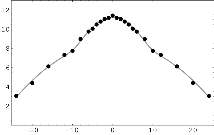
Figure 3: Total number of models as a function of net chirality. The gray line corresponds to the sum of Gaussians $f=A\,e^{-\alpha x^{2}}+B\,e^{-\alpha x^{2}/4}$ where $A=1.64\times 10^{11}$, $B=4.39\times 10^{8}$ and $\alpha=9.13\times 10^{-2}$.

More interestingly we find that the space of $Z_{2}\times Z_{2}$ orbifold models exhibits a novel symmetry under the exchange of the total number of vectorial representations $V$ and the total number of spinorial plus anti–spinorial representations $S_{t}$. Thus, for any given model with a total number of $SO(10)$ $V$–representations, there exist a corresponding model in which the total number of $SO(10)$ $S_{t}$–representations is the same. Below we turn to investigate this symmetry in some detail.

6 Spinor–vector duality

The existence of a $V\leftrightarrow S_{t}$ duality exchange symmetry is apparent when the $SO(10)$ symmetry is enhanced to $E_{6}$. In this case the chiral matter states arise from the $27$ and $\overline{27}$ representations of $E_{6}$, which decompose under $SO(10)$ as

$$27 \equiv 16\oplus 10\oplus 1$$

$$\overline{27} \equiv \overline{16}\oplus 10\oplus 1$$ (6.1)

From eq. (6.1) it is seen that in this case the total number of spinorial $16\oplus{\overline{1}6}$ $SO(10)$ representations is equal to the total number of vectorial $10$ representations, and such models are self–dual under the exchange. Thus, $V\leftrightarrow S_{t}$ duality is trivial in the case of $(2,2)$ Calabi–Yau compactifications. However, over the space of $(2,0)$ vacua that we scan in this work, the $SO(10)$ symmetry is not enhanced to $E_{6}$ symmetry. Nevertheless, the distribution of vacua still exhibits this symmetry. Furthermore, we find that the $V\leftrightarrow S_{t}$ duality holds separately for each twisted plane. In table 2 we illustrate the $V\leftrightarrow S_{t}$ duality on the first plane. The duality is observed by noting that for a fixed number of representations, summing over the number of models with a total number of spinor plus anti–spinor representations produces the identical number of models with the same number of vector representations. Thus, for example, summing over the number of models in the first three rows produces the number of models in the fourth row. Considering that the integral numbers involved are quite high, the resulting equalities are quite astounding!

	First Plane			Second plane			Third Plane
$s$	${\bar{s}}$	$v$	$s$	${\bar{s}}$	$v$	$s$	${\bar{s}}$	$v$	# of models
2	0	0	0	0	0	0	0	0	1325963712
0	2	0	0	0	0	0	0	0	1340075584
1	1	0	0	0	0	0	0	0	3718991872
0	0	2	0	0	0	0	0	0	6385031168
4	0	0	0	0	0	0	0	0	111944544
3	1	0	0	0	0	0	0	0	250947136
2	2	0	0	0	0	0	0	0	1059624448
1	3	0	0	0	0	0	0	0	251936192
0	4	0	0	0	0	0	0	0	113437024
0	0	4	0	0	0	0	0	0	1787889344
0	8	0	0	0	0	0	0	0	535280
2	6	0	0	0	0	0	0	0	8084480
4	4	0	0	0	0	0	0	0	34050304
6	2	0	0	0	0	0	0	0	8053760
8	0	0	0	0	0	0	0	0	529040
0	0	8	0	0	0	0	0	0	51252864
0	16	0	0	0	0	0	0	0	272
4	12	0	0	0	0	0	0	0	9792
6	10	0	0	0	0	0	0	0	26112
8	8	0	0	0	0	0	0	0	84000
10	6	0	0	0	0	0	0	0	26112
12	4	0	0	0	0	0	0	0	9792
16	0	0	0	0	0	0	0	0	272
0	0	16	0	0	0	0	0	0	156352

Table 2: Examples of spinor–vector duality on the first twisted plane. The total number of models with a given number of spinors plus antispinors is equal to the total number of models with the same number of vectors. The total number of models with a given number of spinors plus antispinors is obtained by summing over the different distributions of spinors and antispinors.

Figure 4: Total number of spinors plus antispinors, $S_{t}$, versus the number of vectors, $V$, occurring in the scanned space of vacua.

In figure 4 we display the total number of spinors plus anti–spinors versus the number of vectors occurring in the scan. The figure is clearly symmetric under the exchange of the two axis, which illustrates that for any model with a given number of spinors, anti–spinors and vectors, there is a corresponding model in which the number of vectors is swapped with the number of spinors plus anti–spinors.

In eq. (5) we display in a matrix form the number of models for a given number of vectors and spinors plus anti–spinors. The indices of the raws and columns of the matrix indicate the number of respective representations in the models, whereas the entries are the number of models. In each entry we sum over different configurations by which the spinors, anti–spinor and vector representations are arranged in the three twisted planes and fixed point sectors. Therefore, the entries represent nontrivial sums over different configurations. Examining the matrix in eq. (5) it is seen that it a symmetric matrix reflecting the invariance under exchange of vectors with spinors plus anti–spinors.

Figure 6 is a graphic representation of eq. (5) and shows a density plot of the number of models. The axis of the plot are the number of vectors and the number of spinors plus anti–spinors. The layout of the plot is similar to that of figure 4. The density of the number of models, represented by the gray colouration, exhibits the invariance under exchange of vectors and spinors plus anti–spinors.

Figure 5: Matrix of spinor plus antispinor versus vectors. The entries of the matrix are the total number of models with a given number of spinors and vectors. The symmetry of the matrix manifest the spinor–vector duality.

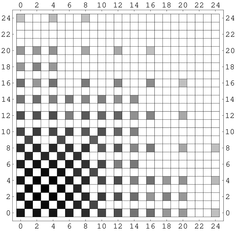
Figure 6: Density plot of the number of models versus the number of vectors and spinors plus anti–spinors.

The $V\leftrightarrow S_{t}$ duality symmetry reflects some modular properties of the $N=1$ partition function. This symmetry arises from a non–trivial discrete torsion induced by reversing some of the GGSO projection coefficients. To illustrate this discrete exchange we consider the simplified model produced by the set of basis vectors

$$v_{1}=1 = \{\psi^{\mu},\ \chi^{1,\dots,6},y^{1,\dots,6},\omega^{1,\dots,6}|$$

$$~{}~{}~{}\bar{y}^{1,\dots,6},\bar{\omega}^{1,\dots,6},\bar{\eta}^{1,2,3},\bar{\psi}^{1,\dots,5},\bar{\phi}^{1,\dots,8}\},$$

$$v_{2}=S = \{\psi^{\mu},\chi^{1,\dots,6}\},$$

$$v_{3}=z_{1} = \{\bar{\phi}^{1,\dots,4}\},$$

$$v_{4}=z_{2} = \{\bar{\phi}^{5,\dots,8}\}.$$

$$v_{5}=x = \{\bar{\psi}^{1,\dots,5},\bar{\eta}^{1,2,3}\},$$

$$v_{6}=b_{1} = \{\chi^{34},\chi^{56},y^{34},y^{56}|\bar{y}^{34},\bar{y}^{56},\bar{\eta}^{1},\bar{\psi}^{1,\dots,5}\},$$ (6.2)

$$v_{7}=b_{2} = \{\chi^{12},\chi^{56},y^{12},\omega^{56}|\bar{y}^{12},\bar{\omega}^{56},\bar{\eta}^{2},\bar{\psi}^{1,\dots,5}\}$$

with the set of one–loop GGSO coefficients

$${\bordermatrix{&1&S&&{z_{1}}&{z_{2}}&{x}&&{b_{1}}&{b_{2}}\cr 1&-1&~{}~{}1&&-1&-1&-1&&-1&-1\cr S&~{}~{}1&~{}~{}1&&-1&-1&-1&&~{}~{}1&~{}~{}1\cr&&&&&&&&&\cr{z_{1}}&-1&-1&&-1&-1&-1&&-1&-1\cr{z_{2}}&-1&-1&&-1&-1&~{}~{}1&&~{}~{}1&~{}~{}1\cr{x}&-1&-1&&-1&~{}~{}1&~{}~{}1&&-1&~{}~{}1\cr&&&&&&&&&\cr{b_{1}}&-1&-1&&-1&~{}~{}1&~{}~{}1&&-1&~{}~{}1\cr{b_{2}}&-1&-1&&-1&~{}~{}1&-1&&~{}~{}1&-1\cr}}$$ (6.3)

The gauge group of this model is $SO(12)\times SO(10)\times U(1)^{3}\times SO(8)\times SO(8)$ and arises solely from the null sector. The gauge bosons arising from all other sectors are projected out. In this model the number of the $SO(10)$ spinorial representations $\#S_{+}=8$ arising from the sector

$$b_{3}\equiv 1+z_{1}+z_{2}+b_{1}+b_{2}~{}.$$

There are no more spinorial representations from the $b_{1}$ sector nor from the $b_{2}$ sector. The sectors $b_{3}+x$ and $b_{1,2}+x+z_{1}$ each, produce eight multiplets that transform in the 8 representation of the hidden $SO(8)_{1}$ gauge group, whereas the sectors $b_{1,2,3}+x+z_{2}$ each, produce eight multiplets that transform in the 8 representation of the hidden $SO(8)_{2}$ gauge group. The sector $z_{2}$ produces a single state that transforms as $8_{\rm v}\otimes 8_{\rm c}$ under $SO(8)_{1}\otimes SO(8)_{2}$.

Switching on a discrete torsion defined by the phase change

$$c{z_{1}\atopwithdelims[ ]b_{1}}=+1\rightarrow c{z_{1}\atopwithdelims[ ]b_{1}}=-1~{},$$ (6.4)

the eight $SO(10)$ spinorial representations from the sector $b_{3}$ are now projected out, whereas the sector $b_{3}+x$ generates eight vectorial 10 representation of $SO(10)$ plus additional $8\times 6$ $SO(10)$ singlets. The remaining observable spectrum, which is charged under $SO(10)$, is identical in these two models, with and without discrete torsion. Hence, the discrete torsion defined in eq. (6.4) induces the duality transformation that exchanges the $SO(10)$ spinorial and vectorial representations. Additionally, the hidden sector matter spectrum is also modified. Indeed, in the presence of torsion the sectors $b_{2}+x$ and $b_{1}+x+z_{2}$ each produce eight multiplets that transform in the 8 representation of the hidden $SO(8)_{2}$ gauge group, whereas the sectors $b_{1,2}+x+z_{1}$ each, produce eight multiplets that transform in the 8 representation of the hidden $SO(8)_{1}$ gauge group. The sector $z_{2}$ produces a single state that transforms as $8_{\rm v}\otimes 8_{\rm c}$ under $SO(8)_{1}\otimes SO(8)_{2}$.

In the next section we present a general proof, based on the solutions of eqs. (3.11), for the $V\leftrightarrow S_{t}$ duality symmetry over the space of vacua.

7 Analytic proof of spinor-vector duality

In section 3 a system of the projection equations (3.11–3.69) that determines the number of spinor and vector representations per twisted plane in algebraic form. This involves the $4\times 4$ binary matrices $\Delta^{(I)}$ of eq. (3.30) and the augmented matrices $\left[\Delta^{(I)},Y_{16}^{(I)}\right]$ and $\left[\Delta^{(I)},Y_{10}^{(I)}\right]$. Since the $V\leftrightarrow S_{t}$ duality interchanges spinors and vectors and since the number of the spinor and vector states relates to the rank of these matrices, as given in eqs. (3.65) and (3.69), we will show that the $V\leftrightarrow S_{t}$ interchange takes place plane by plane. The number of vectorials and spinorials originating from a specific orbifold plane $I$ are interchanged when the ranks of the associated $Y$-vectors are interchanged

$${\rm rank}\left[\Delta^{(I)},Y_{16}^{(I)}\right]\leftrightarrow{\rm rank}\left[\Delta^{(I)},Y_{10}^{(I)}\right]~{},$$ (7.1)

as follows from eqs. (3.65) and (3.69). In order to prove the existence of $V\leftrightarrow S_{t}$ duality we have to demonstrate the existence of a universal map that preserves the ranks of the matrices, while exchanging $Y^{I}_{16}\leftrightarrow Y^{I}_{10}$. Since the rank of the augmented matrix does not change by adding to the $Y^{I}_{10}$ a linear combination of the columns of $\Delta^{I}$ the most general transformations of the GSO phases that realizes the above interchange, modulo the rank preserving transformations, are given by

$$\left(e_{k}\left|b_{1}\right.\right) \rightarrow \left(e_{k}\left|b_{1}+x\right.\right)+\sum_{i=3,4,5,6}\lambda_{i}^{1}\,\left(e_{k}\left|e_{i}\right.\right)\ ,\ k=1,2$$

$$\left(z_{m}\left|b_{1}\right.\right) \rightarrow \left(z_{m}\left|b_{1}+x\right.\right)+\sum_{i=3,4,5,6}\lambda_{i}^{1}\,\left(z_{m}\left|e_{i}\right.\right)\ ,\ m=1,2$$ (7.2)

$$\left(e_{k}\left|b_{2}\right.\right) \rightarrow \left(e_{k}\left|b_{2}+x\right.\right)+\sum_{i=1,2,5,6}\lambda_{i}^{2}\,\left(e_{k}\left|e_{i}\right.\right)\ ,\ k=3,4$$

$$\left(z_{m}\left|b_{2}\right.\right) \rightarrow \left(z_{m}\left|b_{2}+x\right.\right)+\sum_{i=1,2,5,6}\lambda_{i}^{2}\,\left(z_{m}\left|e_{i}\right.\right)\ ,\ m=1,2$$ (7.3)

$$\left(e_{k}\left|b_{3}\right.\right) \rightarrow \left(e_{k}\left|b_{3}+x\right.\right)+\sum_{i=1,2,3,4}\lambda_{i}^{3}\,\left(e_{k}\left|e_{i}\right.\right)\ ,\ k=5,6$$

$$\left(z_{m}\left|b_{3}\right.\right) \rightarrow \left(z_{m}\left|b_{3}+x\right.\right)+\sum_{i=1,2,3,4}\lambda_{i}^{3}\,\left(z_{m}\left|e_{i}\right.\right)\ ,\ m=1,2$$ (7.4)

where $\lambda_{i}^{j}=0,1$ are arbitrary coefficients. The freedom of adding these coefficients amounts to reorganizing the matter spectrum of the vector representations on each twisted plane. Adding these coefficients is necessary, as we show below, in order to prove the existence of a duality map on all three twisted planes. Indeed, the duality map on the first and second planes can be induced by choosing the independent phases $(e_{1,2}|b_{1,2})$ and $(z_{1,2}|b_{1,2})$ arbitrarily, without affecting the $\Delta^{I}$ matrices. In the third plane, however, i.e. for $b_{3}$ which is composed in terms of $b_{1}$ and $b_{2}$, this freedom a priori is not apparent. Replacing $b_{3}=b_{1}+b_{2}+x$ in eq. (7.4) we obtain

$$\left(e_{k}\left|b_{3}\right.\right) \rightarrow \left(e_{k}\left|b_{1}\right.\right)+\left(e_{k}\left|b_{2}\right.\right)+\sum_{i=1,2,3,4}\lambda_{i}^{3}\,\left(e_{k}\left|e_{i}\right.\right)\ ,\ k=5,6$$ (7.5)

$$\left(z_{m}\left|b_{3}\right.\right) \rightarrow \left(z_{m}\left|b_{1}\right.\right)+\left(z_{m}\left|b_{2}\right.\right)+\sum_{i=1,2,3,4}\lambda_{i}^{3}\,\left(z_{m}\left|e_{i}\right.\right)\ ,\ m=1,2$$ (7.6)

The transformation in eq. (7.5) is trivially realized by using the freedom in the phases $\left(e_{5}\left|b_{1}\right.\right)$ and $\left(e_{6}\left|b_{2}\right.\right)$. Turning to the transformation in eq. (7.6), there is no remaining freedom in the choice of the GGSO coefficients $\left(z_{m}\left|b_{1}\right.\right)$ and $\left(z_{m}\left|b_{2}\right.\right)$ since these are used in the transformations on the first two planes. Using the duality transformations in eqs. (7.2-7.4) we may rewrite eq. (7.6) as

$$\left(z_{m}\left|b_{3}\right.\right) \rightarrow \left(z_{1}\left|b_{3}+x\right.\right)+\left[\left(z_{1}\left|z_{2}\right.\right)+1+\sum_{i=1,2}\left(\lambda_{i}^{2}+\lambda_{i}^{3}+1\right)\left(z_{m}\left|e_{i}\right.\right)\right.$$ (7.7)

$$\ \ +\left.\sum_{i=3,4}\left(\lambda_{i}^{1}+\lambda_{i}^{3}+1\right)\left(z_{m}\left|e_{i}\right.\right)+\sum_{i=5,6}\left(\lambda_{i}^{1}+\lambda_{i}^{2}+1\right)\left(z_{m}\left|e_{i}\right.\right)\right]$$

where $m=1,2$ and the identity

$$\left(z_{m}\left|x\right.\right)=\left(z_{m}\left|1+S+z_{1}+z_{2}+\sum_{1}^{6}e_{i}\right.\right)=1+\left(z_{1}\left|z_{2}\right.\right)+\sum_{1}^{6}\left(z_{m}\left|e_{i}\right.\right)$$ (7.8)

is used to obtain eq. (7.7). To show the existence of the duality map on the third twisted plane it is sufficient to demonstrate that the term in the square brackets in eq. (7.7) can be either $0$ or $1$ for appropriate choice of $\lambda_{i}^{j}$ coefficients. This possibility exists provided that at least one of the $\left(z_{1}\left|e_{i}\right.\right)$ and one of the $\left(z_{2}\left|e_{i}\right.\right)$ is non vanishing. This is indeed the case in the class of models that we classify here, being the no gauge group enhancement condition discussed in section 4.

8 Self–dual solutions without enhanced symmetry

In this section we discuss the self dual solutions. The existence of such self dual solutions is evident from the matrix in figure (5 and the density plot in figure 6. The diagonal elements in the figure and the corresponding matrix are the self dual solutions, in which the total number of $(16\oplus{\overline{16}})$ spinorial representations is equal to the total number of $(10)$ vectorial representations of $SO(10)$. This self–duality is obvious when the $SO(10)$ symmetry is enhanced to $E_{6}$. Indeed, in this case the 27 contains the $16+10+1$, whereas the $\overline{27}$ contains the $\overline{16}+10+1$. Hence, in a $E_{6}$ vacuum with a given number of $27$ and $\overline{27}$ the total number of $16\oplus\overline{16}$ spinorial representations is necessarily equal to the total number of $10$ vectorial representations. However, in the models that we classify here the gauge bosons that enhance the $SO(10)\times U(1)$ symmetry to $E_{6}$ are always projected out by the GGSO projections. Nevertheless, as illustrated in 5 and 6, there exist in the space of vacua, models that preserve the self–duality.

In the case that the symmetry is enhanced to $E_{6}$, a given sector $B$, on a given twisted plane, may give rise to a $16$ or $\overline{16}$ representation of $SO(10)$, and necessarily an accompanying $10$ vectorial representation from the sector $B+x$, to supplement the representation to the $27$ representation of $E_{6}$. However, once the $E_{6}$ symmetry is broken we expect that the given sectors $B$ and $B+x$, give rise to either a massless spinor or vector, but not to both, and hence that the equality is removed. Furthermore, as the $E_{6}$ symmetry is broken we anticipate that the Abelian $U(1)$ symmetry in $E_{6}\rightarrow SO(10)\times U(1)$ becomes anomalous. While this expectation is in general correct, there exist models in the space of vacua in which the total numbers of spinor and vectors redistribute themselves among the twisted sectors in a way that maintains the equality of the total number of $(16\oplus\overline{16})$ and $10$ multiplets. In the space of $SO(10)$ vacua classified in our work, these models are self–dual under the spinor–vector duality. Furthermore, in some of these self–dual solutions the Abelian $U(1)$ symmetries are anomalous, whereas in others all the Abelian $U(1)$ symmetries are anomaly free. Below we exhibit two examples of models in this class.

8.1 A three generation self-dual model

This model is generated by the basis vectors $\{v_{1},\dots,v_{12}\}$ of (2.4) and the GGSO coefficients $c{v_{i}\atopwithdelims[ ]v_{j}}=\exp[\left(v_{i}\left|v_{j}\right.\right)]$ , $i,j=1,\dots,12$, where

$$(v_{i}|v_{j})\ \ =\ \ \bordermatrix{&1&S&e_{1}&e_{2}&e_{3}&e_{4}&e_{5}&e_{6}&b_{1}&b_{2}&z_{1}&z_{2}\cr 1&1&1&1&1&1&1&1&1&1&1&1&1\cr S&1&1&1&1&1&1&1&1&1&1&1&1\cr e_{1}&1&1&0&1&0&0&1&0&1&0&0&1\cr e_{2}&1&1&1&0&1&0&1&0&0&0&0&0\cr e_{3}&1&1&0&1&0&0&0&1&0&0&0&0\cr e_{4}&1&1&0&0&0&0&1&0&0&1&1&1\cr e_{5}&1&1&1&1&0&1&0&1&1&1&1&1\cr e_{6}&1&1&0&0&1&0&1&0&1&0&1&0\cr b_{1}&1&0&1&0&0&0&1&1&1&0&1&1\cr b_{2}&1&0&0&0&0&1&1&0&0&1&1&1\cr z_{1}&1&1&0&0&0&1&1&1&1&1&1&1\cr z_{2}&1&1&1&0&0&1&1&0&1&1&0&1\cr}$$

The properties that characterize the model are:

$\bullet$ the gauge group is $SO(10)\times{SO(8)}^{2}\times{U(1)}^{3}$.

$\bullet$ three $SO(10)$ spinorials (one from each plane) arising from the points
$S+b_{1}+e_{3}+e_{5}$, $S+b_{2}+e_{5}$, $S+b_{3}+e_{2}+e_{4}$.

$\bullet$ three $SO(10)$ vectorial representations (one from each plane) arising from
$S+b_{1}+e_{3}+x$, $S+b_{2}+x$ and $S+b_{3}+e_{3}+x$.

$\bullet$ eight octets charged under the first $SO(8)$ arising from
$S+b_{3}+e_{1}+z_{2}$, $S+b_{3}+e_{1}+e_{3}+e_{4}+x$, $S+b_{2}+e_{2}+e_{5}+e_{6}+z_{1}+x$, $S+b_{2}+e_{2}+e_{6}+x$, $S+b_{1}+e_{3}+e_{4}+e_{6}+z_{1}+x$, $S+e_{3}+e_{4}+b_{1}+z_{1}+x$, $S+b_{1}+e_{3}+e_{6}+x$, $S+b_{2}+e_{5}+z_{1}+x$

$\bullet$ eight octets charged under the second ${SO(8)}$ from
$S+b_{3}+e_{3}+e_{4}+z_{2}+x$, $S+b_{3}+e_{4}+e_{5}+e_{6}+x$, $S+b_{3}+e_{1}+e_{2}+e_{3}+z_{2}+x$, $S+b_{2}+e_{1}+e_{5}+x+z_{2}$, $S+b_{2}+e_{1}+x$, $S+b_{1}+e_{3}+e_{4}+e_{6}+x$, $S+b_{1}+e_{4}+e_{5}+e_{6}+x+z_{2}$, $S+b_{2}+x+z_{2}$.

A number of non-Abelian group singlets is also present in the model’s spectrum. All three Abelian factors are anomaly free.

8.2 A six generation self-dual model

This model is generated by the basis vectors $v_{1},\dots,v_{12}$ of (2.4) and the GGSO coefficients $c{v_{i}\atopwithdelims[ ]v_{j}}=\exp[\left(v_{i}\left|v_{j}\right.\right)]$ , $i,j=1,\dots,12$, where

$$(v_{i}|v_{j})\ \ =\ \ \bordermatrix{&1&S&e_{1}&e_{2}&e_{3}&e_{4}&e_{5}&e_{6}&b_{1}&b_{2}&z_{1}&z_{2}\cr 1&1&1&1&1&1&1&1&1&1&1&1&1\cr S&1&1&1&1&1&1&1&1&1&1&1&1\cr e_{1}&1&1&0&0&0&1&0&1&1&0&0&1\cr e_{2}&1&1&0&0&1&1&0&0&0&0&0&0\cr e_{3}&1&1&0&1&0&1&1&0&0&1&1&1\cr e_{4}&1&1&1&1&1&0&0&0&0&1&1&0\cr e_{5}&1&1&0&0&1&0&0&1&0&1&1&1\cr e_{6}&1&1&1&0&0&0&1&0&0&1&1&0\cr b_{1}&1&0&1&0&0&0&0&0&1&0&1&0\cr b_{2}&1&0&0&0&1&1&1&1&0&1&1&0\cr z_{1}&1&1&0&0&1&1&1&1&1&1&1&1\cr z_{2}&1&1&1&0&1&0&1&0&0&0&0&1\cr}$$

The properties that characterize the model are:

$\bullet$ the gauge group is $SO(10)\times{SO(8)}^{2}\times{U(1)}^{3}$.

$\bullet$ six $SO(10)$ spinorials (2 from each plane) arising from the points
$S+b_{1}+e_{6},S+b_{1}+e_{3}+e_{4}+e_{5},S+b_{2}+e_{2}+e_{6},S+b_{2}+e_{1}+e_{5},S+b_{3}+e_{3}+e_{4},$
$S+b_{3}+e_{2}+e_{3}+e_{4}$.

$\bullet$ six $SO(10)$ vectorials (2 from each plane) arising from
$S+b_{1}+e_{3}+e_{4}+e_{6}+x$, $S+b_{2}+e_{1}+e_{6}+x$, $S+b_{2}+e_{2}+e_{5}+x$, $S+b_{2}+e_{5}+x$, $S+b_{3}+e_{1}+e_{3}+e_{4}+x$ , $S+b_{3}+e_{1}+e_{2}+e_{3}+e_{4}+x$.

$\bullet$ six octets charged under the first $SO(8)$ arising from
$S+b_{3}+e_{1}+e_{3}+x$, $S+b_{3}+e_{1}+e_{2}+e_{3}+x$, $S+b_{2}+e_{1}+x$, $S+b_{2}+e_{2}+e_{5}+e_{6}+x$, $S+b_{1}+e_{3}+e_{4}+e_{5}+e_{6}+x+z_{1}$, $S+b_{1}+x+z_{1}$

$\bullet$ six octets charged under the second ${SO(8)}$ from
$S+b_{3}+e1+e4+x+z2$, $S+b_{3}+e_{1}+e_{2}+e_{4}+x+z_{2}$ , $S+b_{2}+e_{1}+e_{5}+e_{6}+z_{2}$, $S+b_{2}+e_{2}+z_{2}$, $S+b_{1}+e_{3}+3_{4}+x+z_{2}$, $S+b_{1}+e_{5}+e_{6}+z_{2}$.

A number of non-Abelian gauge group singlets is also present in the model’s spectrum. All three Abelian factors are anomaly free.

9 Conclusions

In this paper we continued the classification of fermionic $Z_{2}\times Z_{2}$ heterotic string vacua, which was started in ref. [7]. It was restricted in [7] to the models dubbed $S^{3}$ class models, in which all twisted planes may a priori produce spinorial representations. Extensions to $S^{2}V$, $SV^{2}$ and $V^{3}$ classes of models by modifying the set of boundary condition basis vectors were investigated in ref. [8]. However, as discussed in ref. [9] the entire space of $S^{3}$, $S^{2}V$, $SV^{2}$ and $V^{3}$ classes of models is generated by using the single set of basis vectors given in eq. (2.4) and modifying the one–loop GGSO projection. This result follows from theta–functions identities which render the vector basis modification equivalent to certain choices of GGSO projection coefficients in the enlarged basis set (2.4). This equivalence therefore facilitates the classification of this class of string vacua, as one can work with a single basis and the classification entails the variation of the binary GGSO projection coefficients. Counting the number of independent GGSO phases therefore corresponds to a space of $2^{55}$, or approximately $10^{16.6}$, independent choices. In ref. [9] we resorted to a random generation of GGSO phases to scan a space of $\sim 10^{10}$ independent models, with $SO(10)\times U(1)^{3}\times{hidden}$ gauge group. The hidden gauge group in that case was not restricted, and the enhancements of $SO(8)\times SO(8)$ to $SO(16)$ and $E_{8}$ were allowed.

In the work reported here we restricted the classification to models in which the hidden gauge group is not enhanced, and is $SO(10)\times U(1)^{3}\times SO(8)\times SO(8)$ over the entire space of models. This restriction reduced the number of independent phases, and therefore allows the complete classification of this space of vacua, and consequently produces exact results. The classification then reveals a bell shape distribution that peaks at vanishing net number of chiral families, and $\sim 15\%$ of models with three net chiral families. These results are in accordance with the statistical results of ref. [9]. This outcome lends credence to recent attempts [10] at using statistical methods to extract phenomenological information on ensembles of string vacua.

The complete classification revealed a novel duality symmetry over the entire space of scanned vacua under the exchange of spinorial plus antispinorial representations of $SO(10)$ with vectorial representations. This duality symmetry implies that for every model with a given number of spinors (plus antispinors) and vectors there exist another model in which they are interchanged, and reflects a symmetry under the discrete exchange of some GGSO projection coefficients. We exhibited this discrete exchange in one concrete example and provided a general algebraic proof.

It is important to note that over the space of $Z_{2}\times Z_{2}$ heterotic string vacua that we study here the $S_{t}\leftrightarrow V$ duality map operates on the $Z_{2}\times Z_{2}$ twisted planes, plane by plane. As the $Z_{2}\times Z_{2}$ twisted planes preserve $N=2$ space–time supersymmetry this fact implies that the $S_{t}\leftrightarrow V$ duality already exists at the $N=2$ level. It is of interest therefore to explore whether the $S_{t}\leftrightarrow V$ duality also exists in other classes of string compactification do not contain $N=2$ preserving sectors.

The existence of the duality symmetry over the entire space of vacua is of fundamental significance. It reflects the existence of a common structure that underlies the entire space of models. Just as in the case of ten dimensional string theories and eleven dimensional supergravity, the existence of nontrivial duality relations suggests the existence of an underlying theoretical formalism, traditionally dubbed M–theory, the spinor–vector duality indicates a common structure that underlies the entire space of fermionic $Z_{2}\times Z_{2}$ vacua. Thus, the view of this space of string models as consisting of disconnected vacua is premature, and they may in fact be connected by a yet unknown physical mechanism.

It is of further interest to develop a geometrical correspondence of the spinor–vector duality that we uncovered in the free fermionic, or orbifold, limit. In this respect the spinor–vector duality may be viewed as a generalization of the mirror symmetry [13], which exchanges spinors with antispinors. In the geometrical picture, just as mirror symmetry indicated the existence of topology changing transitions between Calabi–Yau manifolds with a mirror Euler characteristic, but equal in absolute value [14], the spinor–vector duality might indicate the existence of topology changing transitions between heterotic string vacua with different Euler character. The geometrical picture in this case, however, might prove more intricate to explore as one must also take account of the vector bundle that accounts for the heterotic string gauge degrees of freedom. Nevertheless, the feasibility of such transitions, afforded by the observation of the spinor–vector duality over the entire space of fermionic $Z_{2}\times Z_{2}$ vacua, suggests that the models in this space are connected by a yet unknown mechanism rather than disconnected.

10 Acknowledgments

We would like to CERN theory division for hospitality. AEF would like to thanks the Oxford theory department for hospitality and is supported in part by PPARC under contract PP/D000416/1. CK is supported in part by the EU under contracts MTRN–CT–2004–005104, MTRN–CT–2004–512194 and ANR (CNRS–USAR) contract No 05–BLAN–0079–01 (01/12/05) JR is supported by the program “PYTHAGORAS” (no. 1705 project 23) of the Operational Program for Education and Initial Vocational Training of the Hellenic Ministry of Education under the 3rd Community Support Framework and the European Social Fund; and by the EU under contract MRTN–CT–2004–503369.

References

- [1] I. Antoniadis, C. Bachas, and C. Kounnas, Nucl. Phys. B289 (1987) 87.
-
[2]
I. Antoniadis, C. Bachas, C. Kounnas and P. Windey, Phys. Lett. B171 (1986) 51;
H. Kawai, D.C. Lewellen, and S.H.-H. Tye, Nucl. Phys. B288 (1987) 1;
I. Antoniadis and C. Bachas, Nucl. Phys. B298 (1988) 586. -
[3]
I. Antoniadis, J. Ellis, J. Hagelin and D.V. Nanopoulos,
Phys. Lett. B231 (1989) 65;
A.E. Faraggi, D.V. Nanopoulos and K. Yuan, Nucl. Phys. B335 (1990) 347;
I. Antoniadis. G.K. Leontaris and J. Rizos, Phys. Lett. B245 (1990) 161;
A.E. Faraggi, Phys. Lett. B278 (1992) 131; Nucl. Phys. B387 (1992) 239;
G.B. Cleaver, A.E. Faraggi and D.V. Nanopoulos, Phys. Lett. B455 (1999) 135;
G.K. Leontaris and J. Rizos, Nucl. Phys. B554 (1999) 3;
A.E. Faraggi, E. Manno and C. Timirgaziu, hep-th/0610118. -
[4]
A.E. Faraggi, Phys. Lett. B326 (1994) 62;
P. Berglund et.al, Phys. Lett. B433 (1998) 269; Int. J. Mod. Phys. A15 (2000) 1345;
R. Donagi and A.E. Faraggi, Nucl. Phys. B694 (2004) 187. -
[5]
E. Kiritsis, C. Kounnas, P.M. Petropoulos and J. Rizos, hep-th/9605011;
E. Kiritsis, C. Kounnas, P.M. Petropoulos and J. Rizos, Nucl. Phys. B483 (1997) 141;
E. Kiritsis and C. Kounnas, Nucl. Phys. B503 (1997) 117;
A. Gregori, C. Kounnas and J. Rizos, Nucl. Phys. B549 (1999) 16;
A. Gregori and C. Kounnas, Nucl. Phys. B560 (1999) 135. - [6] A. Gregori, C. Kounnas and J. Rizos, Nucl. Phys. B549 (1999) 16.
- [7] A.E. Faraggi, C. Kounnas, S.E.M. Nooij and J. Rizos, hep-th/0311058; Nucl. Phys. B695 (2004) 41.
- [8] S.E.M. Nooij, hep-th/0603035, Univ. of Oxford DPhil thesis.
- [9] A.E. Faraggi, C. Kounnas and J. Rizos, hep-th/0606144, Phys. Lett. B, in press.
-
[10]
See e.g.: D. Senechal, Phys. Rev. D39 (1989) 3717;
K.R. Dienes, Phys. Rev. Lett. 65 (1990) 1979; Phys. Rev. D73 (2006) 106010;
M.R. Douglas, JHEP 0305 (2003) 046;
R. Blumenhagen, F. Gmeiner, G. Honecker, D. Lust, and T. Weigand, Nucl. Phys. B713 (2005) 83;
F. Denef and M.R. Douglas, JHEP 0405 (2004) 072;
B.S. Acharya, F. Denef and R. Valadro, JHEP 0506 (2005) 056;
M.R. Douglas and W. Taylor, hep-th/0606109. - [11] C. Vafa an E. Witten, J. Geom. Phys. 15 (1995) 189.
- [12] S. Ashok and M.R. Douglas, JHEP 0401 (2004) 060.
- [13] B.R. Greene and M.R. Plesser, Nucl. Phys. B338 (1990) 15.
-
[14]
P.S. Aspinwall, B.R. Greene and D.R. Morrison,
Nucl. Phys. B416 (1994) 414;
B.R. Greene, D.R. Morrison and A. Strominger, Nucl. Phys. B451 (1995) 109.