Constraints on string networks with junctions

Abstract

We consider the constraints on string networks with junctions in which the strings may all be different, as may be found for example in a network of $(p,q)$ cosmic superstrings. We concentrate on three aspects of junction dynamics. First we consider the propagation of small amplitude waves across a static three-string junction. Then, generalizing our earlier work, we determine the kinematic constraints on two colliding strings with different tensions. As before, the important conclusion is that strings do not always reconnect with a third string; they can pass straight through one another (or in the case of non-abelian strings become stuck in an X configuration), the constraint depending on the angle at which the strings meet, on their relative velocity, and on the ratios of the string tensions. For example, if the two colliding strings have equal tensions, then for ultra-relativistic initial velocities they pass through one another. However, if their tensions are sufficiently different they can reconnect. Finally, we consider the global properties of junctions and strings in a network. Assuming that, in a network, the incoming waves at a junction are independently randomly distributed, we determine the r.m.s. velocities of strings and calculate the average speed at which a junction moves along each of the three strings from which it is formed. Our findings suggest that junction dynamics may be such as to preferentially remove the heavy strings from the network leaving a network of predominantly light strings. Furthermore the r.m.s. velocity of strings in a network with junctions is smaller than $1/\sqrt{2}$, the result for conventional Nambu-Goto strings without junctions in Minkowski spacetime.

I Introduction

The evolution of cosmic string networks and their observational consequences are attracting a great deal of interest, particularly since they may lead to indirect observational tests of superstring theory. The annihilation of two branes at the end of brane inflation Burgess:2001fx ; Dvali:2001fw ; Jones:2002cv ; Kachru:2003aw ; Kachru:2003sx is thought to lead to the formation of cosmic superstrings which can be either fundamental F-strings, Dirichlet D-strings, or $(p,q)$-strings, bound states of the two Dvali:2003zj ; Copeland:2003bj ; Pol ; Firouzjahi:2006vp . Most importantly, the predicted tensions of these strings are not only compatible with current observational bounds ($G\mu\raise 1.29167pt\hbox{$<$\kern-7.5pt\lower 4.30554pt\hbox{$\sim$}}2.3\times 10^{-7}$ using the third year WMAP data Seljak:2006bg ), but they also lie in a window which may be testable with the future LISA gravitational-wave detector ViA1 ; ViA2 ; Irit .

Whilst cosmic superstrings share many of the properties of standard grand unified (GUT) cosmic strings TomMark ; ViSh , they differ in some important respects. First, when two F-strings (or two D-strings) intersect, they do not necessarily ‘intercommute’ — or exchange partners — with probability $P=1$ Jackson:2004zg ; Hanany:2005bc . (An exception for local cosmic strings is when they intercommute at speeds very close to the speed of light Achucarro:2006es .) The effect of reducing $P$ is to increase the density of strings in the final scaling solution and hence the gravity wave signal, though the exact manner in which this happens is under debate ViA1 ; ViA2 ; Sakellariadou:2004wq ; Avgoustidis:2005nv ; Irit . Second, the different kinds of strings in a cosmic superstring network can meet at junctions Tong . Thus when an F and D-sting intersect they cannot intercommute, but rather two junctions are formed and the original strings become connected by a third ($p,q$) bound state. Junctions also exist in non-abelian string networks, for which the fundamental group $\pi_{1}({\cal M})$ of the vacuum manifold ${\cal M}$ is non-abelian.

Even though several authors have addressed both analytically and numerically the cosmological evolution of string networks with junctions Vachaspati:1986cc ; Spergel:1996ai ; Sakellariadou:2004wq ; Martins:2004vs ; Tye:2005fn ; Copeland:2005cy ; Saffin:2005cs ; Hindmarsh:2006qn , the late-time behavior of the network is still not fully understood, particularly when there are different types of string. One possible outcome is that the junctions play a minor rôle and the network reaches a scaling solution similar to that of a GUT string network. In that case it is possible to make predictions for cosmic superstring networks by extracting the information from the GUT string simulations, with suitable allowance for $P\neq 1$ and in principle for different tensions. A second possibility is that the presence of junctions makes the network freeze and eventually dominate the energy density of the universe. Similar questions have been addressed for networks of domain walls with junctions Bucher:1998mh ; Battye:1999eq ; Battye:2005hw ; PinaAvelino:2006ia ; Avelino:2006xy ; Carter:2006cf .

In a previous letter us we studied the dynamics of junctions in a local string network in which the individual strings have no long-range interactions and are well described by the Nambu-Goto action. We set up the equations of motion for three strings of tensions $\mu_{j}$ ($j=1,2,3$) meeting at a junction at position ${\mathbf{X}}(t)$, and were able to solve for the dynamics of ${\mathbf{X}}(t)$ as well as to determine how the junction moved along each of the strings. A related approach has also been developed in the context of representations of baryons as pieces of open string connected at one common point Sharov:1998vy ; 'tHooft:2004he . Having constructed this formalism, we initially presented a simple highly symmetric exact oscillating loop solution. As in the case of ordinary cosmic strings, the existence of exact loop solutions may be important in analyzing the likely behavior of loops in general. Loops of strings with junctions generally evolve rather differently to standard string loops; they do not oscillate periodically and initial analysis indicates that the number of cusps on the loops may be rather different than for conventional Nambu-Goto loops. We intend to return to these points in a future publication.

Our second result concerned the intersection of two strings with equal tensions $\mu_{1}$, meeting at an angle $\alpha$, but with equal and opposite velocities $v$. When these strings collide, for them to exchange partners and become linked by a third string of tension $\mu_{3}$ requires a strong kinematical constraint. We also discussed the case of non-abelian strings, which may become joined by a new string lying along the direction of motion of the two initial strings, and we found the kinematic constraint for this case too.

We expect that these kinematical constraints could have significant consequences on the evolution of string networks with junctions: if the relative velocity of the strings is large, no junction will form and the strings will pass through each other. This in turn means that fewer loops will be formed, and hence that the network would radiate less energy. It may thus be important to include these constraints in analytic and numerical models of network evolution with junctions.

In this paper we extend the work of us , and focus on three aspects of junction dynamics which we believe will be important to understand the global properties of the network. After a review of the equations of motion describing junction evolution in section II, we first consider the propagation of small amplitude waves across a static junction formed of three strings with generally different tensions (section III). Such small waves will inevitably be present on strings in a network, and will radiate gravitationally. We determine the fraction of energy transmitted and reflected across the junction. Then, in sections IV and V, we generalize the kinematic constraints of us to the case in which the two colliding strings have different tensions $\mu_{1}$ and $\mu_{2}$. Since the initial velocity of strings is crucial to determining the importance of the kinematical constraints, in sections VI and VII we consider the global properties of junctions and strings in a network. Assuming that, in a network, the incoming waves at a junction are randomly distributed, we determine the r.m.s. velocities of strings and calculate the average speed at which a junction moves along each of the three strings from which it is formed. Our findings suggest that junction dynamics may be such as to preferentially remove the heavy strings from the network. Finally we conclude in section VIII.

II Review of the basics

We begin by briefly reviewing the equations of motion for strings that form Y junctions obtained in us .

We choose the temporal world-sheet coordinate to be the global time, $\tau=t$, and use the conformal gauge in which the spatial coordinates ${\mathbf{x}}(\sigma,t)$ satisfy

$$\dot{\mathbf{x}}\cdot{\mathbf{x}}^{\prime}=0,\qquad\dot{\mathbf{x}}^{2}+{\mathbf{x}}^{\prime}{}^{2}=1,$$ (1)

where $\dot{\mathbf{x}}=\partial_{t}{\mathbf{x}}$ and ${\mathbf{x}}^{\prime}=\partial_{\sigma}{\mathbf{x}}$. The action for three strings of tensions $\mu_{j}$ ($j=1,2,3$) meeting at a junction is

$$S = -\sum_{j}\mu_{j}\int dt\int d\sigma\,\theta(s_{j}(t)-\sigma)\sqrt{{\mathbf{x}}^{\prime}_{j}{}^{2}(1-\dot{\mathbf{x}}_{j}^{2})}$$ (2)

$$\qquad+\sum_{j}\int dt\,{\mathbf{f}}_{j}(t)\cdot[{\mathbf{x}}_{j}(s_{j}(t),t)-{\mathbf{X}}(t)]$$

where ${\mathbf{X}}(t)$ is the position of the vertex, ${\mathbf{f}}_{j}$ are Lagrange multipliers, and the $s_{j}(t)$ are the values of the spatial world-sheet coordinate at the vertex. It is straightforward to generalize this action to include other vertices, present for example in loop configurations.

Varying ${\mathbf{x}}_{j}$ yields the wave equation, with solution

$${\mathbf{x}}_{j}(\sigma,t)=\frac{1}{2}[{\mathbf{a}}_{j}(\sigma+t)+{\mathbf{b}}_{j}(\sigma-t)],$$ (3)

where, in order to satisfy the gauge conditions (1),

$${\mathbf{a}}^{\prime}_{j}{}^{2}={\mathbf{b}}^{\prime}_{j}{}^{2}=1.$$ (4)

The Lagrange multipliers impose boundary conditions that may be written

$${\mathbf{a}}_{j}(s_{j}+t)+{\mathbf{b}}_{j}(s_{j}-t)=2{\mathbf{X}}(t),$$ (5)

while varying ${\mathbf{X}}$ gives a relation between the Lagrange multipliers which can be reduced to

$$\sum_{j}\mu_{j}[(1+\dot{s}_{j}){\mathbf{a}}^{\prime}_{j}+(1-\dot{s}_{j}){\mathbf{b}}^{\prime}_{j}]={\mathbf{0}}.$$ (6)

Eliminating the ${\mathbf{a}}^{\prime}_{j}$ using the time derivative of (5) then yields

$$\dot{\mathbf{X}}=-\frac{1}{\mu}\sum_{j}\mu_{j}(1-\dot{s}_{j}){\mathbf{b}}^{\prime}_{j},$$ (7)

where

$$\mu=\mu_{1}+\mu_{2}+\mu_{3}.$$ (8)

At the junction, the amplitudes ${\mathbf{b}}^{\prime}_{j}$ of the incoming waves are known from the initial conditions; those of the outgoing waves, ${\mathbf{a}}^{\prime}_{j}$, together with the position of the vertex, are given by (5) and (6), provided the $\dot{s}_{j}$ are known. Finally, the latter may be found by solving the constraint equations ${\mathbf{a}}^{\prime}_{j}{}^{2}=1$. The result depends on the string tensions and on the angles between the unit vectors ${\mathbf{b}}^{\prime}_{j}$. Relative to us , we introduce a slight change of notation, writing for example $c_{1}={\mathbf{b}}^{\prime}_{2}\cdot{\mathbf{b}}^{\prime}_{3}$ (denoted by $c_{23}$ in us ). It will be useful to introduce the quantities $\nu_{j}$ defined, for example, by

$$\nu_{1}=\mu_{2}+\mu_{3}-\mu_{1}.$$ (9)

Then the value of $\dot{s}_{k}$ is given by

$$1-\dot{s}_{k}=\frac{\mu M_{k}(1-c_{k})}{\mu_{k}{\mathcal{M}}},$$ (10)

where the $M_{j}$ are defined by $M_{1}=\nu_{2}\nu_{3}$ along with two similar equations, and

$${\mathcal{M}}=\sum_{j}M_{j}(1-c_{j}).$$ (11)

Notice that since the $\dot{s}_{k}\leq 1$, it follows that the string tensions satisfy triangle inequalities,

$$\nu_{j}\geq 0.$$ (12)

Finally, it follows from (10) that the $\dot{s}_{j}$ satisfy the energy conservation condition

$$\sum_{j}\mu_{j}\dot{s}_{j}=0.$$ (13)

III Small-amplitude waves

A first interesting application of these results is to the reflection and transmission of small-amplitude waves at a junction. Small amplitude waves are expected to build up on strings as a result of self-intersections and interactions with other strings, and they will radiate gravitationally. It is important to understand how they propagate across a junction.

Consider three straight, static strings, for which

$${\mathbf{a}}^{\prime}_{j}={\mathbf{b}}^{\prime}_{j}=(\cos\theta_{j},\sin\theta_{j},0)\equiv{\mathbf{e}}_{j},$$ (14)

with the junction at ${\mathbf{X}}=0$. The equilibrium condition $\dot{s}_{j}=0$ determines the angles between them through (10): for example, we have

$$c_{1}=\cos(\theta_{3}-\theta_{2}) = \frac{\mu_{1}^{2}-\mu_{2}^{2}-\mu_{3}^{2}}{2\mu_{2}\mu_{3}},$$

$$\sin(\theta_{3}-\theta_{2}) = \frac{\Delta}{2\mu_{2}\mu_{3}},$$ (15)

where

$$\Delta=\sqrt{\mu\nu_{1}\nu_{2}\nu_{3}}.$$ (16)

Note that as a consequence of (12), $\Delta$ is real.

Now suppose there is a small incoming perturbation on the first string, so that ${\mathbf{b}}^{\prime}_{1}={\mathbf{e}}_{1}+\delta{\mathbf{b}}^{\prime}_{1}$, with

$$\delta{\mathbf{b}}^{\prime}_{1}(s)=\epsilon{\mathbf{f}}_{1}\cos ks,$$ (17)

where $\epsilon$ is a small dimensionless parameter and ${\mathbf{f}}_{1}$ is a unit vector satisfying ${\mathbf{e}}_{1}\cdot{\mathbf{f}}_{1}=0$; we set $\delta{\mathbf{b}}^{\prime}_{2}=\delta{\mathbf{b}}^{\prime}_{3}={\mathbf{0}}$.

The simplest case is where ${\mathbf{f}}_{1}=(0,0,1)$ since then all $\delta c_{j}=0$, and therefore $\delta\dot{s}_{j}=0$ so that the junction remains at the same value of $\sigma$ on all strings. In that case, the outgoing waves are also in the $z$-direction. From (7) we find

$$\delta\dot{\mathbf{X}}(t)=-\frac{\mu_{1}}{\mu}\epsilon{\mathbf{f}}_{1}\cos kt\,$$ (18)

and hence

$$\delta{\mathbf{a}}^{\prime}_{1}(s) = \frac{\nu_{1}}{\mu}\epsilon{\mathbf{f}}_{1}\cos ks,$$

$$\delta{\mathbf{a}}^{\prime}_{2}(s) = \delta{\mathbf{a}}^{\prime}_{3}(s)=-\frac{2\mu_{1}}{\mu}\epsilon{\mathbf{f}}_{1}\cos ks.$$ (19)

It is then straightforward to find the fraction of energy transmitted along the strings of tension $\mu_{2,3}$ and reflected along the string of tension $\mu_{1}$. Since

$$\delta E_{j}=\frac{\mu_{j}}{4}\int d\sigma(\delta{\mathbf{a}}^{\prime 2}_{j}+\delta{\mathbf{b}}^{\prime 2}_{j}),$$ (20)

we find

$$R_{1}=\frac{\nu_{1}^{2}}{\mu^{2}},\qquad T_{2}=4\frac{\mu_{1}\mu_{2}}{\mu^{2}},\qquad T_{3}=4\frac{\mu_{1}\mu_{3}}{\mu^{2}}.$$ (21)

For instance, suppose that $\mu_{1}\ll\mu_{2}\sim\mu_{3}$, so that the initial perturbation is along the light string. Then, as expected, almost all the energy is essentially reflected off the junction.

The results are more interesting if we take ${\mathbf{f}}_{1}$ in the $xy$-plane, because then the values of $s_{j}$ do oscillate and the junction no longer stays at a fixed position on each string. Let us set

$${\mathbf{f}}_{j}=(-\sin\theta_{j},\cos\theta_{j},0),$$ (22)

so that ${\mathbf{e}}_{j}\cdot{\mathbf{f}}_{j}=0$ for each $j$, and again take $\delta{\mathbf{b}}^{\prime}_{1}$ of the form (17), with $\delta{\mathbf{b}}^{\prime}_{2}=\delta{\mathbf{b}}^{\prime}_{3}={\mathbf{0}}$. Then we have

$$\delta c_{1} = 0,$$

$$\delta c_{2} = -\frac{\Delta}{2\mu_{1}\mu_{3}}\epsilon\cos kt,$$ (23)

$$\delta c_{3} = \frac{\Delta}{2\mu_{1}\mu_{2}}\epsilon\cos kt.$$

It follows that

$$\delta\dot{s}_{1} = \frac{(\mu_{2}-\mu_{3})\nu_{1}}{\Delta}\epsilon\cos kt,$$

$$\delta\dot{s}_{2} = -\frac{\mu_{1}\nu_{1}}{\Delta}\epsilon\cos kt=-\delta\dot{s}_{3}.$$ (24)

Despite this difference, the expressions for the outgoing-wave amplitudes are very similar, except that they are no longer all in the same direction. We find

$$\delta\dot{\mathbf{X}}(t)=\epsilon\cos kt\left(\frac{(\mu_{2}-\mu_{3})\nu_{1}}{\Delta}{\mathbf{e}}_{1}-\frac{\mu_{2}+\mu_{3}}{\mu}{\mathbf{f}}_{1}\right)$$ (25)

from which it follows that

$$\delta{\mathbf{a}}^{\prime}_{1}(s) = -\frac{\nu_{1}}{\mu}\epsilon{\mathbf{f}}_{1}\cos ks$$

$$\delta{\mathbf{a}}^{\prime}_{2}(s) = \frac{2\mu_{1}}{\mu}\epsilon{\mathbf{f}}_{2}\cos ks,$$ (26)

$$\delta{\mathbf{a}}^{\prime}_{3}(s) = \frac{2\mu_{1}}{\mu}\epsilon{\mathbf{f}}_{3}\cos ks.$$

The fact that the amplitudes of the outgoing waves are the same in magnitude independent of the orientation of ${\mathbf{f}}_{1}$ is at first sight remarkable, but actually it follows from the fact that we can regard the waves as representing massless particles propagating along the strings. The amplitudes of the outgoing waves can be derived from conservation of energy and momentum. It follows that the reflection and transmission coefficients are as given in (21), a result that has also been obtained in the more general setting of multivolume junctions by Fomin:2000tv .

Comparing (24) with (26), one interesting point emerges: in the first case, ${\mathbf{a}}^{\prime}_{1}$ is in phase with ${\mathbf{b}}^{\prime}_{1}$, whereas in the second case it is in anti-phase. This means that if the incoming wave is at an intermediate angle, the reflected wave is tilted in the opposite direction.

IV Collisions of straight strings

Figure 1: Two colliding strings, of unequal tension, joined by a third string (an $x$-link).

As summarized in the introduction, in us we discussed the collision of two straight strings of equal tension, $\mu_{1}=\mu_{2}$, and derived kinematical constraints on such a process. Here we wish to extend this discussion to the case of unequal tension, and hence it will be useful to define

$$\mu_{+}\equiv\mu_{1}+\mu_{2},\qquad\mu_{-}\equiv\mu_{1}-\mu_{2}.$$ (27)

Since $\nu_{i}\geq 0$, $\mu_{3}$ is bounded by

$$\mu_{-}\leq\mu_{3}\leq\mu_{+}.$$ (28)

This extension is non-trivial as the problem now lacks the symmetry associated with the equal tension case, and as a first step one must determine the orientation and velocity of the joining string after the collision. This is the aim of the present section.

Consider two strings of tension $\mu_{1}$ and $\mu_{2}$ parallel to the $xy$-plane but at angles $\pm\alpha$ to the $x$-axis, and approaching each other with velocities $\pm v$ in the $z$-direction. Before the collision (for $t<0$, see Fig. 1) we take

$${\mathbf{x}}_{1,2}(\sigma,t)=(-\gamma^{-1}\sigma\cos\alpha,\mp\gamma^{-1}\sigma\sin\alpha,\pm vt),$$ (29)

where $\gamma^{-1}=\sqrt{1-v^{2}}$. Thus

$${\mathbf{a}}^{\prime}_{1,2} = (-\gamma^{-1}\cos\alpha,\mp\gamma^{-1}\sin\alpha,\pm v),$$

$${\mathbf{b}}^{\prime}_{1,2} = (-\gamma^{-1}\cos\alpha,\mp\gamma^{-1}\sin\alpha,\mp v).$$ (30)

At the collision, $t=0$, we suppose that the strings interchange partners. Now, since $\mu_{-}\neq 0$, we can no longer conclude that the third – joining – string formed after the two original strings exchange partners, will be static and that it will lie either along the $x$- or $y$-axis. It is still true that this third string must be parallel to the $xy$-plane and that there are two orientations for it, depending on which ends of the original strings are joined to each other. To be specific, let us assume that the two ends in the positive-$x$ region are joined at a new vertex, ${\mathbf{X}}$, while those in the negative-$x$ region are joined to the other end of the new string which has tension $\mu_{3}$. We call this an $x$-link — see Figure 1. (The corresponding $y$-link is obtained by replacing $\alpha\rightarrow(\pi/2-\alpha)$ and will be discussed below.)

The new string of tension $\mu_{3}$ thus lies at an angle $\theta$ to the $x$ axis, and moves in the $z$-direction with some velocity $u$; thus

$${\mathbf{x}}_{3}(\sigma,t)=(\gamma_{u}^{-1}\sigma\cos\theta,\gamma_{u}^{-1}\sigma\sin\theta,ut),$$ (31)

where $\gamma_{u}=1/\sqrt{1-u^{2}}$. We now determine $\theta$ and $u$. It follows from (31) that

$${\mathbf{b}}^{\prime}_{3}=(\gamma_{u}^{-1}\cos\theta,\gamma_{u}^{-1}\sin\theta,-u),$$ (32)

and thus

$$c_{1} = -\gamma_{u}^{-1}\gamma^{-1}\cos(\alpha+\theta)-uv,$$

$$c_{2} = -\gamma_{u}^{-1}\gamma^{-1}\cos(\alpha-\theta)+uv,$$ (33)

$$c_{3} = 2\gamma^{-2}\cos^{2}\alpha-1.$$

The position of the vertex is of course ${\mathbf{X}}(t)={\mathbf{x}}_{3}(s_{3}(t),t)$, so from (31),

$$\dot{\mathbf{X}}=(\dot{s}_{3}\gamma_{u}^{-1}\cos\theta,\dot{s}_{3}\gamma_{u}^{-1}\sin\theta,u).$$ (34)

Thus, from (7) and (10), we obtain

$${\mathcal{M}}\dot{\mathbf{X}}+M_{3}(1-c_{3}){\mathbf{b}}^{\prime}_{3}=-M_{1}(1-c_{1}){\mathbf{b}}^{\prime}_{1}-M_{2}(1-c_{2}){\mathbf{b}}^{\prime}_{2},$$ (35)

whose three components are

$$[{\mathcal{M}}\dot{s}_{3}+M_{3}(1-c_{3})]\gamma_{u}^{-1}\cos\theta = [M_{1}(1-c_{1})+M_{2}(1-c_{2})]\gamma^{-1}\cos\alpha,$$

$${[{\mathcal{M}}\dot{s}_{3}+M_{3}(1-c_{3})]}\gamma_{u}^{-1}\sin\theta = [M_{1}(1-c_{1})-M_{2}(1-c_{2})]\gamma^{-1}\sin\alpha,$$ (36)

$${[{\mathcal{M}}-M_{3}(1-c_{3})]}u = [M_{1}(1-c_{1})-M_{2}(1-c_{2})]v.$$

Dividing the $y$-component of (36) by the $x$-component, and comparing with the $z$-component gives

$$\frac{\tan\theta}{\tan\alpha}=\frac{u}{v}=\frac{M_{1}(1-c_{1})-M_{2}(1-c_{2})}{M_{1}(1-c_{1})+M_{2}(1-c_{2})}.$$ (37)

The first equality here allows us to eliminate $\theta$. The second, combined with (33), then allows us to obtain an equation for $u$, which simplifies to a quadratic for $u^{2}$ (see Appendix A):

$$\mu_{-}^{2}(\sin^{2}\alpha)u^{4} + [\mu_{3}^{2}(1-v^{2})+\mu_{-}^{2}(v^{2}\cos^{2}\alpha-\sin^{2}\alpha)]u^{2}$$ (38)

$$- \mu_{-}^{2}v^{2}\cos^{2}\alpha=0.$$

This equation always has one positive root which then determines $\theta$ from (37). Notice that when $\mu_{-}=0$ as in us , then $u=0$ and $\theta=0$: this is the symmetric case. On the other hand, in the limit when the bound in (28) is saturated, i.e., $\mu_{-}^{2}\to\mu_{3}^{2}$, then $u\to v$ and $\theta\to\alpha$. Also, when $v\rightarrow 1$ for $\mu_{-}>0$, then $u\rightarrow 1$ and again $\theta\rightarrow\alpha$.

The intercommutation produces kinks on the original strings, moving along them at the speed of light; they are in fact at the same positions as in the equal tension case, namely at

$$K_{1,2}=(\gamma^{-1}\cos\alpha,\pm\gamma^{-1}\sin\alpha,\pm v)t.$$ (39)

V Kinematic constraints

Having found the orientation and velocity of the connecting string, the physical condition that the junctions must move apart imposes the requirement

$$\dot{s}_{3}>0$$ (40)

where $\dot{s}_{3}$ is given in (10). This in turn implies kinematic constraints on the values of $v$ and $\alpha$ of the colliding strings for which an $x$-link can be formed. Replacing $\alpha$ by $\pi/2-\alpha$ gives a similar condition for the formation of a $y$-link.

When $\mu_{-}=0$, constraint (40) reproduces the results of us , namely

$$\alpha<\arccos\left(\frac{\mu_{3}\gamma}{2\mu_{1}}\right) (x\mathrm{-link})$$ (41)

$$\alpha>\arcsin\left(\frac{\mu_{3}\gamma}{2\mu_{1}}\right) (y\mathrm{-link}).$$ (42)

If these bounds are not satisfied, then abelian strings presumably pass through one another. Essentially this same result, in the special case of all tensions equal $\mu_{1}=\mu_{2}=\mu_{3}$, was obtained earlier in the context of hadronic strings Artru , and also when $\mu_{-}=0$ from a different starting point in the context of Type-I strings BK .

For non-abelian strings, as discussed in us , there is a third possibility namely that a link forms in the direction of motion of the two initial strings (a $z$-link). Indeed if the string fluxes on strings 1 and 2 do not commute, then for topological reasons the strings cannot simply pass through one another: they may only do so with the formation of a third string. Note that in this case we do not have strings with three different tensions meeting at a vertex: at one end of string 3 it is attached to two segments of string 1, and at the other to two segments of string 2. Hence the linking string in this case does lie along the $z$-axis, simplifying the analysis. In effect, we have two vertices of the type discussed in us . The triangle inequalities (12) now require that both ${\mu_{3}}\leq 2\mu_{1}$ and $\mu_{3}\leq{2\mu_{2}}$. Furthermore the kinematic constraint in this case is that the total length of string 3 must increase; we must add the rates from the two ends. It is not absolutely necessary that $\dot{s}_{3}$ at one particular vertex should be positive. The required condition is

$$\frac{2\mu_{1}v-\mu_{3}}{2\mu_{1}-\mu_{3}v}+\frac{2\mu_{2}v-\mu_{3}}{2\mu_{2}-\mu_{3}v}>0.$$ (43)

Solving for $v$ gives the limit

$$v>\frac{4\mu_{1}\mu_{2}+\mu_{3}^{2}-\sqrt{(4\mu_{1}^{2}-\mu_{3}^{2})(4\mu_{2}^{2}-\mu_{3}^{2})}}{2(\mu_{1}+\mu_{2})\mu_{3}}.$$ (44)

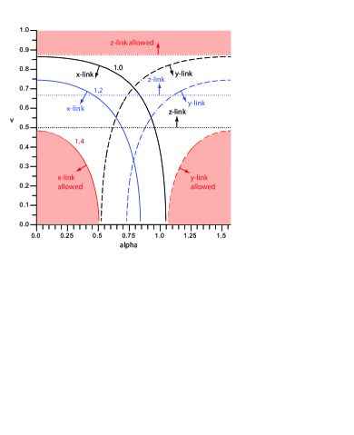
These different constraints are summarized in Figures 2 and 3 showing the $(\alpha,v)$ plane for $\mu=3$. Fig. 2 shows the three constraints for the case $\mu_{-}=0$ (equations (41), (42) and (44)) and various values of $\mu_{3}$ (distinguished by color). For non-abelian strings there are three different regimes: i) if $\mu_{3}>\sqrt{2}\mu_{1}$ there is a kinematically forbidden region for all $\alpha$; ii) for $2\mu_{1}/\sqrt{3}>\mu_{3}>\sqrt{2}\mu_{1}$ only a restricted range of $\alpha$ are forbidden; iii) for $\mu_{3}<2\mu_{1}/\sqrt{3}$ the whole $(\alpha,v)$ plane is included in at least one of the allowed regions. Allowed regions for the formation of an $x$-link are to the left of the solid lines, those for a $y$-link to the right of the dashed lines, while for a $z$-link in the non-abelian case they are above the horizontal dotted lines.

Figure 2: Kinematic constraints for $\mu_{-}=0$. Allowed regions for $x$-links are to the left of the full curves; for $y$-links to the right of the dashed curves; and, for $z$-links in the non-abelian case, above the horizontal dotted lines. The values of $\mu_{3}$ are 1.4 (red), 1.2 (blue), 1.0 (black). Allowed regions are shaded for the $\mu_{3}=1.4$ case.

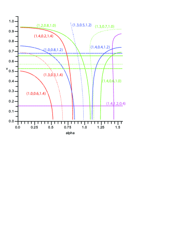
Fig. 3 shows the allowed regions for a number of cases with $\mu_{-}>0$. (The sign of $\mu_{-}$ does not affect the limits.) The allowed $x$-link regions are to the left of the curves, and those for a $z$-link above the horizontal lines. (The $y$-link regions can be found by the substitution $\alpha\to\pi/2-\alpha$.)

Figure 3: Kinematic constraints for strings of unequal tensions normalized to $\mu=3$ for the formation of $x$- and $z$ links. The allowed region is to the left of the $x$-link curves. For $z$-links, it is above the horizontal line (which is absent if $\mu_{3}>2\mu_{2}$). The values of $\mu_{3}$ are again color-coded. The values of $(\mu_{1},\mu_{2},\mu_{3})$ shown are: $(1.0,0.6,1.4)$, red, dashed; $(1.3,0.3,1.4)$, red, dotted; $(1.4,0.2,1.4)$, red, solid; $(1.0,0.8,1.2)$, blue, dashed; $(1.3,0.5,1.2)$, blue, dotted; $(1.4,0.4,1.2)$, blue, solid; $(1.2,0.8,1.0)$, green, dashed; $(1.3,0.7,1.0)$, green, dotted; $(1.4,0.6,1.0)$, green, solid; $(1.4,1.2,0.4)$, magenta, solid.

When $\mu_{-}\neq 0$, it does not seem to be possible to solve (40) analytically for all $\alpha$. We note, however, that there are certain limiting cases for which an analytic solution is possible. Firstly, in the low-velocity limit, $v\to 0$, it is clear from (38) that also $u\to 0$. In this limit, $\sin\theta=(\mu_{-}/\mu_{3})\sin\alpha$. It is then straightforward to show that an $x$-link is only possible if

$$\sin^{2}\alpha_{(v=0)}<\frac{\mu_{+}^{2}-\mu_{3}^{2}}{\mu_{+}^{2}-\mu_{-}^{2}}.$$ (45)

Note that the value of $\alpha$ increases if $\mu_{3}$ decreases, or if $\mu_{-}$ increases. [Recall that the triangle inequalities impose the restrictions (28).]

We can also find a solution for $\alpha=0$. Here $u$ is readily obtainable from (38) and then (40) yields

$$v_{(\alpha=0)}^{2}<\frac{\mu_{3}^{2}(\mu_{+}^{2}-\mu_{3}^{2})}{\mu_{+}^{2}(\mu_{3}^{2}-\mu_{-}^{2})}\equiv v_{c}^{2}.$$ (46)

Thus $v_{c}$ defined in (46) increases with $\mu_{-}^{2}$. Both these limits indicate that in general the kinematic constraints exclude a smaller region of the $(\alpha,v)$ plane as the string tensions become more different. This behavior is readily seen in Fig. 3.

In the equal tension case, $\mu_{-}=0$, $v_{c}$ is always less than 1. Here, however, $v_{c}^{2}\leq 1$ only if

$$\mu_{3}^{2}\geq\mu_{+}\mu_{-}=|\mu_{1}^{2}-\mu_{2}^{2}|.$$ (47)

If this condition is satisfied by the tension of the potentially linking string, there is a velocity $v_{c}$ above which abelian strings will necessarily pass through each other rather than intercommuting. However, when the condition is violated, the entire high-velocity region $v\to 1$ for all $\alpha$ is included in the allowed region. The bounding curve in this case bends to the right, and reaches $\alpha=\pi/2$ at a finite velocity, above which an $x$-link is kinematically allowed for any angle $\alpha$. This velocity constraint for $\alpha=\pi/2$ is

$$v_{(\alpha=\pi/2)}^{2}>\frac{\mu_{+}^{2}(\mu_{3}^{2}-\mu_{-}^{2})}{\mu_{3}^{2}(\mu_{+}^{2}-\mu_{3}^{2})}.$$ (48)

Note that this limit is equal to $1/v_{c}^{2}$.

VI Rate of change of string lengths

One of the important reasons for studying the kinematics of string collisions is that the results may throw some light on the question of how a network of such strings would evolve in the early universe. If we ignore the Hubble expansion and any energy loss mechanisms, then the energy in the string network is fixed, but some strings will shorten and others will grow. We may ask how fast, on average, is this growth or shortening.

It is reasonable to assume that at any string junction, the unit vectors ${\mathbf{b}}^{\prime}_{j}$ representing the ingoing waves are randomly distributed on the unit sphere, and mutually independent. (This might not be true if for example two of the strings come from the same other vertex, but that is presumably not a common situation.) If the strings are all of the same tension, then because of energy conservation it is clear that $\langle\dot{s}_{j}\rangle$ must vanish for each $j$, but this is not necessarily so if the tensions are different. And as we shall see, even for the equal-tension case, the zero mean does not mean that the distribution is symmetrical; it is actually not true that strings are as likely to grow as to shrink.

Let us start by looking at the distribution of the variables $c_{j}$, assuming that the unit vectors ${\mathbf{b}}^{\prime}_{j}$ are randomly distributed on the unit sphere, and mutually independent. Let us choose the $z$-axis along the direction of ${\mathbf{b}}^{\prime}_{3}$, and ${\mathbf{b}}^{\prime}_{2}$ in the ($x,z)$ plane; ${\mathbf{b}}^{\prime}_{2}=(\sin\theta,0,\cos\theta)$. Then ${\mathbf{b}}^{\prime}_{1}=(\sin\beta\cos\phi,\sin\beta\sin\phi,\cos\beta)$ and we may assume a uniform distribution in the variables $c_{1},c_{2}$ and $\phi$ where

$$c_{3}=c_{1}c_{2}+\sqrt{1-c_{1}^{2}}\sqrt{1-c_{2}^{2}}\cos\phi.$$ (49)

Our aim is to calculate the probability distribution for, say, the rate $\dot{s}_{1}$ at which the first string grows. Specifically, let $P(\dot{s}_{1})d\dot{s}_{1}$ be the probability that $\dot{s}_{1}$ lies between $\dot{s}_{1}$ and $\dot{s}_{1}+d\dot{s}_{1}$. Clearly,

$$P(\dot{s}_{1}) = \frac{1}{8\pi}\int_{-1}^{1}dc_{1}\int_{-1}^{1}dc_{2}\int_{0}^{2\pi}d\phi$$ (50)

$$\times\delta\left(\dot{s}_{1}-1+\frac{\mu M_{1}(1-c_{1})}{\mu_{1}{\mathcal{M}}}\right),$$

where we have used (10), and ${\mathcal{M}}={\mathcal{M}}(c_{1},c_{2},c_{3})$ is defined in (11).

The resulting calculation is fairly lengthy, so we relegate the details to Appendix B. The distribution $P(\dot{s}_{1})$ takes three different analytic forms in three intervals, namely

$$1. -1<\dot{s}_{1}<\frac{\mu_{3}^{2}-\mu_{1}^{2}-\mu_{2}^{2}}{2\mu_{1}\mu_{2}};$$

$$2. \frac{\mu_{3}^{2}-\mu_{1}^{2}-\mu_{2}^{2}}{2\mu_{1}\mu_{2}}<\dot{s}_{1}<\frac{\mu_{2}^{2}-\mu_{1}^{2}-\mu_{3}^{2}}{2\mu_{1}\mu_{3}};$$ (51)

$$3. \frac{\mu_{2}^{2}-\mu_{1}^{2}-\mu_{3}^{2}}{2\mu_{1}\mu_{3}}<\dot{s}_{1}<1.$$

(Without loss of generality, we have chosen $\mu_{2}\geq\mu_{3}$.) To write the final expressions for the probability distribution concisely, it is useful to introduce the constant

$$Q=\frac{\mu}{3\nu_{1}\nu_{2}\nu_{3}}.$$ (52)

Then the expressions for $P(\dot{s}_{1})$ in the three regions are

$$1. P(\dot{s}_{1})=Q\mu^{2}\mu_{1}^{2}\left(\frac{1+\dot{s}_{1}}{1-\dot{s}_{1}}\right)^{2}\frac{(2\mu_{2}+2\mu_{3}-\mu_{1})+(2\mu_{1}-\mu_{2}-\mu_{3})\dot{s}_{1}}{(\mu_{1}\dot{s}_{1}+\mu_{2}+\mu_{3})^{3}};$$

$$2. P(\dot{s}_{1})=Q\nu_{2}^{2}\frac{(2\mu_{1}+\mu_{2}-\mu_{3})}{\mu_{1}(1-\dot{s}_{1})^{2}};$$ (53)

$$3. P(\dot{s}_{1})=Q\mu_{1}^{2}\nu_{1}^{2}\frac{(\mu_{1}+2\mu_{2}+2\mu_{3})+(2\mu_{1}+\mu_{2}+\mu_{3})\dot{s}_{1}}{(\mu_{1}\dot{s}_{1}+\mu_{2}+\mu_{3})^{3}}.$$

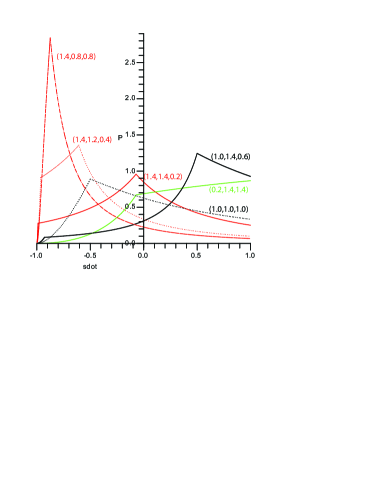
The probability distribution has kinks at the boundaries between these regions, given by (53). The form of the distribution is illustrated for various cases in Fig. 4.

Figure 4: The distribution of $P(\dot{s}_{1}$) plotted against $\dot{s}_{1}$. The values of $\mu_{1}$ are indicated by colors. The curves shown are for $(\mu_{1},\mu_{2},\mu_{3})=(1.4,0.8,0.8)$, red, dashed; $(1.4,1.2,0.4)$, red, dotted; $(1.4,1.4,0.2)$, red, solid; $(1.0,1.0,1.0)$, black, dotted; $(1.0,1.4,0.6)$, black, solid; $(0.2,1.4,1.4)$, green, solid.

In the particular case where the tensions are all equal, the distribution has a single kink, at $\dot{s}_{1}=-\frac{1}{2}$. Its form is

$$1. P(\dot{s}_{1})=\frac{27}{(\dot{s}_{1}+2)^{3}}\left(\frac{1+\dot{s}_{1}}{1-\dot{s}_{1}}\right)^{2}\qquad\left(\dot{s}_{1}<-\frac{1}{2}\right)$$

$$3. P(\dot{s}_{1})=\frac{4\dot{s}_{1}+5}{(\dot{s}_{1}+2)^{3}}\qquad\left(\dot{s}_{1}>-\frac{1}{2}\right).$$

It is interesting that although the mean value of $\dot{s}_{1}$ in this distribution is zero, as it must be, the distribution is not symmetrical — the dotted black curve in Figure 4. At any particular time, it is most probable that one of the three legs is growing, while the other two are shrinking (of course at a slower rate).

More generally, if $\mu_{2}=\mu_{3}$, there is only a single kink; three of the curves in Fig. (4) are examples of this case, with $\mu_{1}=1.4$, 1.0, and 0.2.

It is now straightforward (if tedious) to compute the average value of $\dot{s}_{1}$. We find

$$\langle\dot{s}_{1}\rangle = \frac{3\mu_{1}-\mu}{3\mu_{1}}+\frac{Q}{\mu_{1}}\biggl{[}-(\mu_{1}+\mu)\nu_{1}^{2}\ln\frac{\mu\nu_{1}}{4\mu_{2}\mu_{3}}$$ (54)

$$+(\mu_{1}+\nu_{3})\nu_{2}^{2}\ln\frac{\mu\nu_{2}}{4\mu_{1}\mu_{3}}$$

$$+(\mu_{1}+\nu_{2})\nu_{3}^{2}\ln\frac{\mu\nu_{3}}{4\mu_{1}\mu_{2}}\biggr{]}.$$

Note that the expression (54) is symmetrical under the interchange $\mu_{2}\leftrightarrow\mu_{3}$, as it should be. It is also easy to check that it satisfies the consistency condition

$$\mu_{1}\langle\dot{s}_{1}\rangle+\mu_{2}\langle\dot{s}_{2}\rangle+\mu_{3}\langle\dot{s}_{3}\rangle=0.$$ (55)

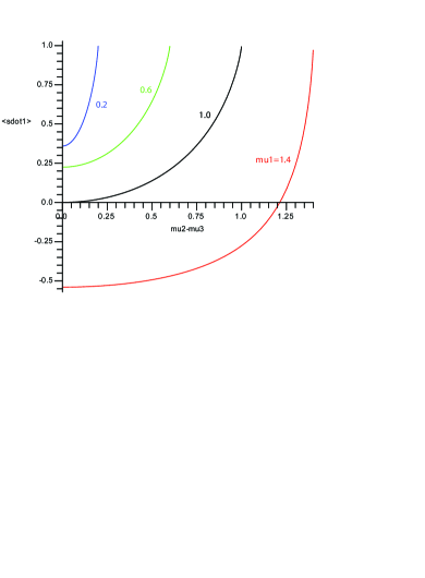
Finally it is interesting to note that in general $\langle\dot{s}_{1}\rangle$ is more likely to be positive if $\mu_{1}$ is small, or if the other two tensions are very different. In Fig. 5, the average value is plotted against $|\mu_{2}-\mu_{3}|$ for various values of $\mu_{1}$. Notice that for $\mu_{1}\leq 1$, $\langle\dot{s}_{1}\rangle$ is always positive. It appears that in a network of strings there may be tendency for the lighter strings to grow at the expense of the heavier ones. This seems to be consistent with results obtained by studying the statistical mechanics of such networks of strings RS .

Figure 5: Average value of $\dot{s}_{1}$ plotted against $|\mu_{2}-\mu_{3}|$ for $\mu_{1}=0.2$ (blue), 0.6 (green), 1.0 (black) and 1.4 (red).

VII Average string velocity

For ordinary Nambu-Goto strings in flat space-time, the r.m.s. transverse string velocity in a random tangle of strings is $1/\sqrt{2}$. It is interesting to ask whether this figure would be different for junction-forming strings. It is easy in principle to answer this question. For example the square of the velocity of the first string adjacent to the vertex is

$$\dot{\mathbf{x}}_{1}^{2}=\frac{1}{2}(1-{\mathbf{a}}^{\prime}_{1}\cdot{\mathbf{b}}^{\prime}_{1}),$$ (56)

and using (5) and (7) this can be expressed in terms of the $c_{j}$. We have

$$(1+\dot{s}_{1}){\mathbf{a}}^{\prime}_{1}\cdot{\mathbf{b}}^{\prime}_{1} = \frac{\nu_{1}}{\mu}(1-\dot{s}_{1})-\frac{2\mu_{2}}{\mu}(1-\dot{s}_{2})c_{3}$$ (57)

$$-\frac{2\mu_{3}}{\mu}(1-\dot{s}_{3})c_{2}.$$

Using (10) this becomes

$${\mathbf{a}}^{\prime}_{1}\cdot{\mathbf{b}}^{\prime}_{1}=\frac{\nu_{1}M_{1}(1-c_{1})-2\mu_{1}M_{2}(1-c_{2})c_{3}-2\mu_{1}M_{3}(1-c_{3})c_{2}}{-\nu_{1}M_{1}(1-c_{1})+2\mu_{1}M_{2}(1-c_{2})+2\mu_{1}M_{3}(1-c_{3})}.$$ (58)

We can then compute the average over the probability distribution already obtained by plugging this expression into an integral of the same form as (50). In this case, there does not seem to be any obvious way of obtaining an analytic result, but it is possible to make some progress. It seems to be slightly easier to compute the average of ${\mathbf{x}}^{\prime}{}^{2}$ rather than $\dot{\mathbf{x}}^{2}$:

$$\langle{\mathbf{x}}^{\prime}_{1}{}^{2}\rangle = \frac{1}{2}\langle 1+{\mathbf{a}}^{\prime}_{1}\cdot{\mathbf{b}}^{\prime}_{1}\rangle$$

$$= \left\langle\frac{2\mu_{1}^{2}(1-c_{2})(1-c_{3})}{-M_{1}(1-c_{1})+2\mu_{1}[\nu_{3}(1-c_{2})+\nu_{2}(1-c_{3})]}\right\rangle.$$

Then if we use as independent variables $c_{2},c_{3},\psi$ with now

$$c_{1}=c_{2}c_{3}+\sqrt{1-c_{2}^{2}}\sqrt{1-c_{3}^{2}}\cos\psi,$$ (60)

we can perform the $\psi$ integration, to yield

$$\langle{\mathbf{x}}^{\prime}_{1}{}^{2}\rangle=\frac{\mu_{1}^{2}}{2}\int_{-1}^{1}dc_{2}\int_{-1}^{1}dc_{3}\frac{(1-c_{2})(1-c_{3})}{\sqrt{F^{2}-G^{2}}},$$ (61)

where

$$F=2\mu_{1}[\nu_{3}(1-c_{2})+\nu_{2}(1-c_{3})]-\nu_{2}\nu_{3}(1-c_{2}c_{3}),$$ (62)

and

$$G=\nu_{2}\nu_{3}\sqrt{1-c_{2}^{2}}\sqrt{1-c_{3}^{2}}.$$ (63)

Remarkably (61) can be evaluated to give the general result

$$\langle\dot{\bf x}_{1}^{2}\rangle = \langle(1-{\mathbf{x}}^{\prime}_{1}{}^{2})\rangle$$ (64)

$$= \frac{\mu_{1}^{2}-13\bar{\mu}^{2}}{15(\mu_{1}^{2}-\bar{\mu}^{2})}+\frac{(4\mu_{1}-\bar{\mu})(\mu_{1}+\bar{\mu})^{2}}{15\mu_{1}(\mu_{1}-\bar{\mu})^{2}}\ln\frac{2\mu_{1}}{\mu_{1}+\bar{\mu}}$$

$$+\frac{(4\mu_{1}+\bar{\mu})(\mu_{1}-\bar{\mu})^{2}}{15\mu_{1}(\mu_{1}+\bar{\mu})^{2}}\ln\frac{2\mu_{1}}{\mu_{1}-\bar{\mu}},$$

where we have introduced $\bar{\mu}=\mu_{2}-\mu_{3}$. A number of interesting features can be seen. First, the result is independent of $\mu_{2}+\mu_{3}$, depending only on the single ratio $\bar{\mu}/\mu_{1}$. Secondly, the limit $\bar{\mu}=0$ gives

$$\langle\dot{\bf x}_{1}^{2}\rangle=\frac{1}{15}\left[1+8\ln 2\right]\simeq 0.436,$$ (65)

independently of $\mu_{1}$. In particular we note that, even for strings of equal tension, the r.m.s. velocity is not $1/\sqrt{2}$ as it is for ordinary Nambu-Goto strings without junctions. Surprisingly, on the contrary, this value is obtained when $\bar{\mu}=\mu_{1}$, a limit in which the triangle inequality is only just satisfied.

For completeness, in Fig. 6 we have plotted $v_{\rm rms}=\sqrt{\langle\dot{\bf x}_{1}^{2}\rangle}$, for various choices of $\mu_{1}$, a function of $|\mu_{2}-\mu_{3}|$.

Figure 6: R.m.s. value of the string velocity $v$ plotted against $|\mu_{2}-\mu_{3}|$ for several values of $\mu_{1}$.

VIII Conclusions

In an earlier letter us , we considered the kinematic constraints on the possibility of intercommuting of strings that form junctions. Concentrating on the case where the approaching strings have equal tensions, we showed that if the relative velocity with which they meet is too large, no exchange can take place and the strings will pass through one another (or, for non-abelian strings, become joined by a string in the direction of the relative velocity or form a linked X configuration). In this paper we have extended the analysis to the more realistic case where the approaching strings have different tensions. For some values of the string tensions, it may happen that ultra-relativistic strings can exchange partners.

We first studied the reflection and transmission of small-amplitude waves at string junctions — something that may be important in predicting the gravitational radiation from strings. We determined the fraction of energy transmitted and reflected across the junction, and showed how the reflected wave is generally tilted in the opposite direction to the incoming wave.

In sections IV and V, we generalized the kinematic constraints (41) and (42) of I to the case in which the two colliding strings have different tensions $\mu_{1}$ and $\mu_{2}$. The question of whether strings always intercommute is vital in understanding the evolution of a network of strings; in particular it affects the final density of strings found in the scaling regime of a network, if indeed a scaling solution is reached. We have established the criteria required for intercommuting in terms of the incoming velocity and angle of approach, as a function of the string tensions. A particularly important combination of tensions is that given in the inequality (47). If this inequality is satisfied, for instance when $\mu_{1}=\mu_{2}$, then ultra-relativistic strings cannot intercommute. If it is violated, then ultra-relativistic strings may intercommute. Our result that intercommuting does not always happen appears at first sight to be in contrast to the claim in Eto:2006db , but we believe the regime where their results are applicable corresponds to low velocities of approach as the moduli approximation they use breaks down for high velocities. It is in the high velocity regime that intercommutation may break down.

Since the initial velocity of colliding strings is crucial to determining the importance of the kinematical constraints, in sections VI and VII we considered the global properties of junctions and strings in a network. A plausible assumption for a string network is that the incoming waves at a junction are randomly distributed. This has allowed us to make progress in determining the r.m.s. velocites of strings. In particular (ignoring energy loss mechanisms such as expansion of the universe) we have calculated the average speed at which a junction moves along each of the three strings from which it is formed. Our results are intriguing. For example, even for the case of equal tension strings, although the average velocity of the junctions is zero as expected, the distribution of the velocities is not peaked around zero, but around a negative velocity (actually around $\dot{s_{i}}=-1/2$) indicating that even in this apparently symmetric case, it is most probable that at any particular time, one of the three legs is growing, while the other two are shrinking, all be it at a slower rate. The case of unequal tensions can also be solved analytically and our results suggest that junction dynamics may be such as to preferentially remove the heavy strings from the network. It thus seems likely that the system will evolve to one where the lightest strings are dominating the dynamics, though of course junctions are still present. Regarding the r.m.s. velocities of the strings themselves, we showed that they are generically smaller than the $1/\sqrt{2}$ characteristic of Nambu-Goto networks, even in the case when the strings all have equal tensions.

In a future publication we intend to present some exact solutions for loops containing junctions. Given the new features we have uncovered for the dynamics of string networks with junctions, we should not be surprised to find important results concerning the distribution of kinks and cusps in these more complicated configurations. This in turn could have a bearing on the gravitational radiation emitted from loops of strings with junctions.

APPENDIX A

Here we outline the calculation of equation (38). Let $\mu_{\pm}=\mu_{1}\pm\mu_{2}$, so that

$$M_{1,2}=(\mu_{+}-\mu_{3})(\mu_{3}\pm\mu_{-}),\qquad M_{3}=\mu_{3}^{2}-\mu_{-}^{2}.$$

Then the second equality in (37) yields

$$\frac{u}{v}=\qquad\qquad\qquad\qquad\qquad\qquad\qquad\qquad\qquad\qquad\qquad$$

$$\frac{\mu_{-}(1+\gamma^{-1}\gamma_{u}^{-1}\cos\alpha\cos\theta)+\mu_{3}(uv-\gamma^{-1}\gamma_{u}^{-1}\sin\alpha\sin\theta)}{\mu_{3}(1+\gamma^{-1}\gamma_{u}^{-1}\cos\alpha\cos\theta)+\mu_{-}(uv-\gamma^{-1}\gamma_{u}^{-1}\sin\alpha\sin\theta)}.$$

Next we can eliminate $\cos\theta$ and $\sin\theta$. ¿From the first equality in (37),

$$\cos\theta = \frac{v\cos\alpha}{\sqrt{v^{2}\cos^{2}\alpha+u^{2}\sin^{2}\alpha}},$$

$$\sin\theta = \frac{u\sin\alpha}{\sqrt{v^{2}\cos^{2}\alpha+u^{2}\sin^{2}\alpha}}.$$

Thus multiplying up and grouping all the terms involving $\gamma^{-1}$ on the right, gives

$$(\mu_{3}u-\mu_{-}v)+(\mu_{-}u-\mu_{3}v)uv=$$

$$\frac{\gamma^{-1}\gamma_{u}^{-1}}{\sqrt{v^{2}\cos^{2}\alpha+u^{2}\sin^{2}\alpha}}[(\mu_{-}v-\mu_{3}u)v\cos^{2}\alpha+$$

$$\qquad\qquad\qquad(\mu_{-}u-\mu_{3}v)u\sin^{2}\alpha].$$

Now square to obtain

$$(v^{2}\cos^{2}\alpha+u^{2}\sin^{2}\alpha)[\mu_{3}u(1-v^{2})-\mu_{-}v(1-u^{2})]^{2}=$$

$$-(1-v^{2})(1-u^{2})[\mu_{-}(v^{2}\cos^{2}\alpha+u^{2}\sin^{2}\alpha)-\mu_{3}uv]^{2}.$$

On expansion, the terms in $uv$, which come from the cross terms in each square bracket, cancel, and we are left with

$$F\left[\mu_{3}^{2}u^{2}(1-v^{2})-\mu_{-}^{2}(1-u^{2})(v^{2}\cos^{2}\alpha+u^{2}\sin^{2}\alpha)\right]=0$$

where

$$F=(1-v^{2})(v^{2}\cos^{2}\alpha+u^{2}\sin^{2}\alpha)-v^{2}(1-u^{2})$$

which vanishes only if $v=\pm u$. Thus we finally get the quadratic (38) for $u^{2}$:

$$\mu_{-}^{2}(\sin^{2}\alpha)u^{4} + [\mu_{3}^{2}(1-v^{2})+\mu_{-}^{2}(v^{2}\cos^{2}\alpha-\sin^{2}\alpha)]u^{2}$$

$$- \mu_{-}^{2}v^{2}\cos^{2}\alpha=0.$$

This always has one positive root as the discriminant is positive.

APPENDIX B

To carry out the integral in Eq. (50), it is convenient to go over to a more symmetrical form by changing variable from $\phi$ to $c_{3}$, using (49). This introduces a Jacobian factor, which is the inverse of

$$\frac{dc_{3}}{d\phi}=-\sqrt{1-c_{1}^{2}}\sqrt{1-c_{2}^{2}}\sin\phi=-\sqrt{J},$$

where

$$J = (1-c_{1}^{2})(1-c_{2}^{2})-(c_{3}-c_{1}c_{2})^{2}$$

$$= 1-c_{1}^{2}-c_{2}^{2}-c_{3}^{2}+2c_{1}c_{2}c_{3}.$$

Note that the physically allowed region in $(c_{1},c_{2},c_{3})$ space is characterized by $J\geq 0$. There is also a factor of $2$ because there are two values of $\phi$ for each $c_{3}$. Letting $w_{1}=1-\dot{s}_{1}$, we arrive at

$$P(1-w_{1}) = \frac{1}{4\pi}\int_{-1}^{1}dc_{1}\int_{-1}^{1}dc_{2}\int_{-1}^{1}dc_{3}\frac{\theta(J)}{\sqrt{J}}$$ (66)

$$\times\delta\left(w_{1}-\frac{\mu M_{1}(1-c_{1})}{\mu_{1}{\mathcal{M}}}\right).$$

It is straightforward to perform the $c_{3}$ integral using the delta function. This gives

$$P(1-w_{1})=\frac{1}{4\pi}\frac{\mu}{\mu_{1}}\frac{M_{1}}{M_{3}}\frac{1}{w_{1}^{2}}\int_{-1}^{1}dc_{1}(1-c_{1})\int_{-1}^{1}dc_{2}\frac{\theta(J)}{\sqrt{J}},$$ (67)

where now

$$J=(1-c_{1}^{2})(1-c_{2}^{2})-[c_{3}(w_{1})-c_{1}c_{2}]^{2}.$$ (68)

Here $c_{3}(w_{1})$ is obtained by equating to zero the argument of the delta function in (67) and solving for $c_{3}$:

$$c_{3}(w_{1})=1+\frac{M_{1}}{M_{3}}(1-c_{1})\left(1-\frac{\mu}{\mu_{1}w_{1}}\right)+\frac{M_{2}}{M_{3}}(1-c_{2}).$$ (69)

Now since, by (68), $J$ is a quadratic function of $c_{2}$, we can go on to perform the $c_{2}$ integral in (67). It is clear from (68) that $J\leq 0$ when $c_{2}=\pm 1$, so the effective limits of integration for the $c_{2}$ integral are given by the roots of $J=0$. If there are no real roots, the contribution is zero. Specifically, $J$ has the form

$$J=\frac{1}{M_{3}^{2}}(A+2Bc_{2}-Kc_{2}^{2}),$$ (70)

where

$$A=(1-c_{1}^{2})M_{3}^{2}-H^{2},$$

$$B=(M_{2}+c_{1}M_{3})H,$$ (71)

$$K=M_{2}^{2}+M_{3}^{2}+2c_{1}M_{2}M_{3},$$

with

$$H=M_{2}+M_{3}-(1-c_{1})Y,$$ (72)

where

$$Y=M_{1}\left(\frac{\mu}{\mu_{1}w_{1}}-1\right).$$ (73)

Note that by the triangle inequality, $Y$ is positive. The discriminant, which determines whether real roots exist, is

$$B^{2}+AK=(1-c_{1}^{2})(K-H^{2})=(1-c_{1}^{2})D,$$ (74)

say. If the roots are $c_{2\pm}$, then the $c_{2}$ integral reduces to

$$\int_{c_{2-}}^{c_{2+}}\frac{dc_{2}}{\sqrt{J}}=\frac{\pi M_{3}}{\sqrt{K}}.$$ (75)

Thus

$$P(1-w_{1})=\frac{\mu M_{1}}{4\mu_{1}w_{1}^{2}}\int_{-1}^{1}dc_{1}\frac{(1-c_{1})}{\sqrt{K}}\theta(D)$$ (76)

Now from (71)–(73),

$$D = (M_{2}+M_{3})^{2}-2(1-c_{1})M_{2}M_{3}$$ (77)

$$-[M_{2}+M_{3}-(1-c_{1})Y]^{2}$$

$$= (1-c_{1})[-2M_{2}M_{3}$$

$$+2(M_{2}+M_{3})Y-(1-c_{1})Y^{2}].$$

It is useful to change variable from $c_{1}$ to $\xi$ defined by

$$\xi^{2}=K=(M_{2}+M_{3})^{2}-2(1-c_{1})M_{2}M_{3}.$$ (78)

The range of values of $\xi$ corresponding to $-1<c_{1}<1$ is then

$$|M_{2}-M_{3}|<\xi<M_{2}+M_{3}.$$ (79)

For convenience, we shall assume in what follows that $\mu_{2}\geq\mu_{3}$, so the lower limit is $M_{2}-M_{3}$. The effect of the condition that the square bracket in (77) be positive is to require that

$$\xi>\xi_{c}=\frac{|(M_{2}+M_{3})Y-2M_{2}M_{3}|}{Y}.$$ (80)

Hence

$$P(1-w_{1})=\frac{\mu M_{1}}{4\mu_{1}w_{1}^{2}}\int_{\xi_{-}}^{\xi_{+}}\frac{\xi d\xi}{M_{2}M_{3}}\frac{(M_{2}+M_{3})^{2}-\xi^{2}}{2M_{2}M_{3}\xi},$$ (81)

where

$$\xi_{+} = M_{2}+M_{3},$$

$$\xi_{-} = \max(\xi_{c},M_{2}-M_{3}).$$ (82)

The integral (81) can be rewritten as

$$P(1-w_{1})=\frac{\mu M_{1}}{8\mu_{1}M_{2}^{2}M_{3}^{2}w_{1}^{2}}\int_{\xi_{-}}^{\xi_{+}}(\xi_{+}^{2}-\xi^{2})d\xi,$$ (83)

and hence evaluated to yield the final result

$$P(1-w_{1})=\frac{\mu M_{1}}{24\mu_{1}M_{2}^{2}M_{3}^{2}}\frac{(\xi_{+}-\xi_{-})^{2}(2\xi_{+}+\xi_{-})}{w_{1}^{2}}.$$ (84)

We must distinguish three different ranges of values of $w_{1}$ corresponding to the following ranges of $Y$:

$$1. 0<Y<M_{3},\qquad\xi_{-}=\frac{2M_{2}M_{3}}{Y}-(M_{2}+M_{3});$$

$$2. M_{3}<Y<M_{2},\qquad\xi_{-}=M_{2}-M_{3};$$ (85)

$$3. M_{2}<Y,\qquad\xi_{-}=(M_{2}+M_{3})-\frac{2M_{2}M_{3}}{Y};$$

It is straightforward to rewrite the distribution in terms of the string tensions $\mu_{j}$ and the variable $\dot{s}_{1}$. The values of $\dot{s}_{1}$ corresponding to the three ranges are easily seen to be those in (51), and the corresponding expressions for $P(\dot{s}_{1})$ are given in (53).

References

• (1) C. P. Burgess, M. Majumdar, D. Nolte, F. Quevedo, G. Rajesh and R. J. Zhang, JHEP 0107, 047 (2001) [arXiv:hep-th/0105204].
• (2) G. R. Dvali, Q. Shafi and S. Solganik, arXiv:hep-th/0105203.
• (3) N. T. Jones, H. Stoica and S. H. H. Tye, JHEP 0207, 051 (2002) [arXiv:hep-th/0203163].
• (4) S. Kachru, R. Kallosh, A. Linde and S. P. Trivedi, Phys. Rev. D 68, 046005 (2003) [arXiv:hep-th/0301240].
• (5) S. Kachru, R. Kallosh, A. Linde, J. M. Maldacena, L. McAllister and S. P. Trivedi, JCAP 0310, 013 (2003) [arXiv:hep-th/0308055].
• (6) G. Dvali and A. Vilenkin, JCAP 0403, 010 (2004) [arXiv:hep-th/0312007].
• (7) E. J. Copeland, R. C. Myers and J. Polchinski, JHEP 0406, 013 (2004) [arXiv:hep-th/0312067].
• (8) J. Polchinski, AIP Conf. Proc.  743, 331 (2005) [Int. J. Mod. Phys. A 20, 3413 (2005)] [arXiv:hep-th/0410082].
• (9) H. Firouzjahi, L. Leblond and S. H. Henry Tye, JHEP 0605, 047 (2006) [arXiv:hep-th/0603161].
• (10) U. Seljak, A. Slosar and P. McDonald, arXiv:astro-ph/0604335.
• (11) T. Damour and A. Vilenkin, Phys. Rev. D 64, 064008 (2001) [arXiv:gr-qc/0104026].
• (12) T. Damour and A. Vilenkin, Phys. Rev. D 71, 063510 (2005) [arXiv:hep-th/0410222].
• (13) X. Siemens, J. Creighton, I. Maor, S. Ray Majumder, K. Cannon and J. Read, Phys. Rev. D 73, 105001 (2006) [arXiv:gr-qc/0603115].
• (14) M. B. Hindmarsh and T. W. B. Kibble, Rept. Prog. Phys.  58, 477 (1995) [arXiv:hep-ph/9411342].
• (15) A. Vilenkin and E. P. S. Shellard, Cosmic Strings and other Topological Defects (Cambridge University Press, Cambridge, 1994).
• (16) M. G. Jackson, N. T. Jones and J. Polchinski, JHEP 0510, 013 (2005) [arXiv:hep-th/0405229].
• (17) A. Hanany and K. Hashimoto, JHEP 0506, 021 (2005) [arXiv:hep-th/0501031].
• (18) A. Achucarro and R. de Putter, arXiv:hep-th/0605084.
• (19) M. Sakellariadou, JCAP 0504, 003 (2005) [arXiv:hep-th/0410234].
• (20) A. Avgoustidis and E. P. S. Shellard, arXiv:astro-ph/0512582.
• (21) K. Hashimoto and D. Tong, JCAP 0509, 004 (2005) [arXiv:hep-th/0506022].
• (22) T. Vachaspati and A. Vilenkin, Phys. Rev. D 35, 1131 (1987).
• (23) D. Spergel and U. L. Pen, Astrophys. J.  491, L67 (1997) [arXiv:astro-ph/9611198].
• (24) C. J. A. Martins, Phys. Rev. D 70, 107302 (2004) [arXiv:hep-ph/0410326].
• (25) S. H. Henry Tye, I. Wasserman and M. Wyman, Phys. Rev. D 71, 103508 (2005); ibid. 71, 129906(E) (2005) [arXiv:astro-ph/0503506].
• (26) E. J. Copeland and P. M. Saffin, JHEP 0511, 023 (2005) [arXiv:hep-th/0505110].
• (27) P. M. Saffin, JHEP 0509, 011 (2005) [arXiv:hep-th/0506138].
• (28) M. Hindmarsh and P. M. Saffin, JHEP 0608, 066 (2006) [arXiv:hep-th/0605014].
• (29) M. Bucher and D. N. Spergel, Phys. Rev. D 60, 043505 (1999) [arXiv:astro-ph/9812022].
• (30) R. A. Battye, M. Bucher and D. Spergel, arXiv:astro-ph/9908047.
• (31) R. A. Battye, B. Carter, E. Chachoua and A. Moss, Phys. Rev. D 72, 023503 (2005) [arXiv:hep-th/0501244].
• (32) P. Pina Avelino, C. J. A. Martins, J. Menezes, R. Menezes and J. C. R. Oliveira, Phys. Rev. D 73, 123519 (2006) [arXiv:astro-ph/0602540].
• (33) P. P. Avelino, C. J. A. Martins, J. Menezes, R. Menezes and J. C. R. Oliveira, Phys. Rev. D 73, 123520 (2006) [arXiv:hep-ph/0604250].
• (34) B. Carter, arXiv:hep-ph/0605029.
• (35) E. J. Copeland, T. W. B. Kibble and D. A. Steer, Phys. Rev. Lett.  97 (2006) 021602 [arXiv:hep-th/0601153].
• (36) G. S. Sharov, arXiv:hep-ph/9809465.
• (37) G. ’t Hooft, arXiv:hep-th/0408148.
• (38) P. I. Fomin and Yu. V. Shtanov, Class. Quant. Grav.  19, 3139 (2002) [arXiv:hep-th/0008183].
• (39) X. Artru, Nucl. Phys.  B 85 (1975) 442.
• (40) L. M. A. Bettencourt and T. W. B. Kibble, Phys. Lett.  B 332 (1994) 297 [arXiv:hep-ph/9405221].
• (41) M. Eto, K. Hashimoto, G. Marmorini, M. Nitta, K. Ohashi and W. Vinci, arXiv:hep-th/0609214.
• (42) R. J. Rivers and D. A. Steer, Statistical mechanics of strings with Y junctions, work in progress, 2006.