hep-th/0611242

NORDITA-2006-11-20

Magnetic Heisenberg-chain/pp-wave correspondence

Troels Harmark$\,{}^{1}$, Kristjan R. Kristjansson$\,{}^{2}$ and Marta Orselli$\,{}^{2}$

¹ The Niels Bohr Institute
Blegdamsvej 17, 2100 Copenhagen Ø, Denmark

² Nordita
Blegdamsvej 17, 2100 Copenhagen Ø, Denmark

harmark@nbi.dk, kristk@nordita.dk, orselli@nbi.dk

Abstract

We find a decoupling limit of planar $\mathcal{N}=4$ super Yang-Mills (SYM) on $\mathbb{R}\times S^{3}$ in which it becomes equivalent to the ferromagnetic $XXX_{1/2}$ Heisenberg spin chain in an external magnetic field. The decoupling limit generalizes the one found in hep-th/0605234 corresponding to the case with zero magnetic field. The presence of the magnetic field is seen to break the degeneracy of the vacuum sector and it has a non-trivial effect on the low energy spectrum. We find a general connection between the Hagedorn temperature of planar $\mathcal{N}=4$ SYM on $\mathbb{R}\times S^{3}$ in the decoupling limit and the thermodynamics of the Heisenberg chain. This is used to study the Hagedorn temperature for small and large value of the effective coupling. We consider the dual decoupling limit of type IIB strings on $\mbox{AdS}_{5}\times S^{5}$. We find a Penrose limit compatible with the decoupling limit that gives a magnetic pp-wave background. The breaking of the symmetry by the magnetic field on the gauge theory side is seen to have a geometric counterpart in the derivation of the Penrose limit. We take the decoupling limit of the pp-wave spectrum and succesfully match the resulting spectrum to the low energy spectrum on the gauge theory side. This enables us to match the Hagedorn temperature of the pp-wave to the Hagedorn temperature of the gauge theory for large effective coupling. This generalizes the results of hep-th/0608115 to the case of non-zero magnetic field.

1 Introduction

The AdS/CFT correspondence conjectures that $\mathcal{N}=4$ $SU(N)$ super Yang-Mills (SYM) on $\mathbb{R}\times S^{3}$ is equivalent to type IIB string theory on $\mbox{AdS}_{5}\times S^{5}$ [1, 2, 3]. In [4, 5] a new decoupling limit of AdS/CFT was introduced. The limit is most naturally expressed as a limit of the thermal partition functions on both sides of the correspondence. On the gauge theory side, the limit is [4]

$$\Omega\rightarrow 1,\quad\tilde{T}\equiv\frac{T}{1-\Omega}\ \mbox{fixed},\quad\tilde{\lambda}\equiv\frac{\lambda}{1-\Omega}\ \mbox{fixed},\quad N\ \mbox{fixed},$$ (1.1)

where $T$ is the temperature, $\Omega=\Omega_{1}=\Omega_{2}$, $\Omega_{3}=0$ with $\Omega_{i}$ being the chemical potentials corresponding to the three R-charges $J_{i}$, $i=1,2,3$, for the $SU(4)$ R-symmetry of $\mathcal{N}=4$ SYM. Also, $\lambda$ is the ’t Hooft coupling and $N$ is the rank of the gauge group. In the limit (1.1) all states except for the ones in the $SU(2)$ sector decouple. In fact, the full partition function of $\mathcal{N}=4$ SYM on $\mathbb{R}\times S^{3}$ reduces to ($\tilde{\beta}=1/\tilde{T}$)

$$Z(\tilde{\beta})=\mathop{{\rm Tr}}\left(e^{-\tilde{\beta}(D_{0}+\tilde{\lambda}D_{2})}\right)$$ (1.2)

where the trace is over the $SU(2)$ sector only, and the $D_{0}$ and $D_{2}$ operators come from the weak coupling expansion of the dilatation operator $D=D_{0}+\lambda D_{2}+\mathcal{O}(\lambda^{3/2})$, with $D_{0}$ being the bare term and $D_{2}$ the one-loop term. For planar $\mathcal{N}=4$ SYM the $\tilde{\lambda}D_{2}$ term for single-traces of a fixed length corresponds to the Hamiltonian of the ferromagnetic $XXX_{1/2}$ Heisenberg spin chain with zero magnetic field. Thus, weakly coupled planar $\mathcal{N}=4$ SYM in the limit (1.1) is equivalent to the Heisenberg chain.

On the dual string theory side the limit is instead in terms of the angular velocities $\Omega_{i}$ on the five-sphere, the string tension $T_{\rm str}$ and the string coupling $g_{s}$. It takes the form [5]

$$\Omega\rightarrow 1,\quad\tilde{T}\equiv\frac{T}{1-\Omega}\ \mbox{fixed},\quad\tilde{T}_{\rm str}\equiv\frac{T_{\rm str}}{\sqrt{1-\Omega}}\ \mbox{fixed},\quad\tilde{g}_{s}\equiv\frac{g_{s}}{1-\Omega}\ \mbox{fixed},$$ (1.3)

again with $\Omega=\Omega_{1}=\Omega_{2}$ and $\Omega_{3}=0$. We see that the limit (1.3) involves taking the string tension $T_{\rm str}$ and the string coupling $g_{s}$ to zero. Therefore, the decoupling limit of AdS/CFT found in [4, 5] leads to a correspondence between a decoupled sector of weakly coupled $\mathcal{N}=4$ SYM and weakly coupled string theory.

If we in particular consider planar $\mathcal{N}=4$ SYM then this is dual to free type IIB string theory on $\mbox{AdS}_{5}\times S^{5}$, and the decoupling limit gives us therefore in this case a triality between the Heisenberg chain, a limit of weakly coupled $\mathcal{N}=4$ SYM and a zero tension limit of free string theory on $\mbox{AdS}_{5}\times S^{5}$. In [5] this was tested for large $\tilde{\lambda}$ and large $J=J_{1}+J_{2}$, with the successful result that the spectra of the gauge theory and string theory sides match. On the gauge theory side the spectrum corresponds to the spectrum of magnons in the Heisenberg chain. On the string theory side the spectrum is obtained from taking the decoupling limit of the spectrum for a particular pp-wave background. The matching of the spectra furthermore leads to the result that the Hagedorn temperature, as computed on the gauge theory/spin chain side, matches with the Hagedorn temperature computed on the string theory side for the pp-wave background, for large $\tilde{\lambda}$ [5].

That the Hagedorn temperature on the gauge theory and string theory sides are dual to each other has been proposed in [6, 7, 8, 9]. The result of [5] thus finds a region of AdS/CFT where it can be checked explicitly that the Hagedorn temperatures indeed match.

In this paper we consider a modification of the decoupling limit (1.1) for $\mathcal{N}=4$ SYM on $\mathbb{R}\times S^{3}$ such that it becomes equivalent to the ferromagnetic Heisenberg $XXX_{1/2}$ spin chain in an external magnetic field. We have again $\Omega_{3}=0$ and we define $\Omega=(\Omega_{1}+\Omega_{2})/2$ and $h=(\Omega_{1}-\Omega_{2})/2$. The new decoupling limit is then

$$\Omega\rightarrow 1,\quad\tilde{T}\equiv\frac{T}{1-\Omega}\ \mbox{fixed},\quad\tilde{h}\equiv\frac{h}{1-\Omega}\ \mbox{fixed},\quad\tilde{\lambda}\equiv\frac{\lambda}{1-\Omega}\ \mbox{fixed},\quad N\ \mbox{fixed}.$$ (1.4)

This limit reduces to (1.1) when $\tilde{h}=0$. The full partition function of $\mathcal{N}=4$ SYM on $\mathbb{R}\times S^{3}$ now reduces to

$$Z(\tilde{\beta},\tilde{h})=\mathop{{\rm Tr}}\left(e^{-\tilde{\beta}(D_{0}+\tilde{\lambda}D_{2}-2\tilde{h}S_{z})}\right)$$ (1.5)

where the trace is, as before, over the $SU(2)$ sector. For planar $\mathcal{N}=4$ SYM the $\tilde{\lambda}D_{2}-2\tilde{h}S_{z}$ part of the Hamiltonian corresponds to the Hamiltonian of the ferromagnetic $XXX_{1/2}$ Heisenberg spin chain with a magnetic field of magnitude $2\tilde{h}$.

For the zero magnetic field case (1.2) the Heisenberg chain $\tilde{\lambda}D_{2}$ has a degenerate vacuum sector. In fact there is a vacuum state for each value of the total spin $S_{z}$. The introduction of the magnetic field in (1.5) gives the interesting effect that the degeneracy is broken and only a single vacuum remains. As we explain in the main text, this is fundamental to the understanding of the physics of $\mathcal{N}=4$ SYM in the modified limit (1.4). In particular, it is responsible for a non-trivial modification of the spectrum for large $\tilde{\lambda}$ and $J$, and it also gives a non-trivial effect for the Hagedorn temperature.

On the string theory side we obtain again the spectrum from a decoupling limit of the spectrum of a particular pp-wave background. For the zero magnetic field this pp-wave background is the maximally supersymmetric pp-wave background [10], however, not in the coordinate system used in the gauge-theory/pp-wave correspondence of BMN [11], but instead in a coordinate system where the pp-wave background has a flat direction, i.e. an explicit isometry [12, 13]. This flat direction corresponds to the degenerate vacuum sector on the gauge theory side [5]. The flat direction pp-wave background can be seen as the BMN pp-wave background rotated with constant angular velocity in a plane with the critical velocity for which the quadratic terms disappear. With the magnetic field, the pp-wave background instead corresponds to rotating with a constant angular velocity that is near the critical angular velocity.

Since we are not at the critical angular velocity the explicit isometry of the flat direction is broken. This is the string dual version of the breaking of the degeneracy of the vacuum sector on the gauge theory side caused by the magnetic field. We observe that for this reason the decoupled sector of the near-critical pp-wave used in this paper resembles much more the pp-wave background used by BMN than the pp-wave with a flat direction.

The pp-wave background with a near-critical angular velocity can also be seen as a magnetic pp-wave background, in the sense that the off-diagonal terms in the metric are analogous to a magnetic field. We therefore dub the background a magnetic pp-wave background, so in this sense we can say that we have obtained a correspondence between the magnetic Heisenberg chain and a magnetic pp-wave background.

We match successfully both the spectrum and the Hagedorn temperature as found from the gauge-theory/spin-chain side and from the string theory side. This provides a new example of a direct correspondence between a sector of weakly coupled gauge theory and free string theory which can be seen as an extension of that of Ref. [5].

2 Gauge theory side: The magnetic Heisenberg chain

In this section we introduce a new decoupling limit of thermal $\mathcal{N}=4$ super Yang-Mills (SYM) on $\mathbb{R}\times S^{3}$ in which $\mathcal{N}=4$ SYM reduces to a quantum mechanical theory on the $SU(2)$ sector. This limit can be seen as a generalization of the $SU(2)$ decoupling limit found in [4]. We show that in the decoupling limit, planar $\mathcal{N}=4$ SYM becomes equivalent to the ferromagnetic $XXX_{1/2}$ Heisenberg spin chain with a magnetic field. This should be contrasted to the $SU(2)$ decoupling limit of [4] in which planar $\mathcal{N}=4$ SYM is equivalent to the Heisenberg chain without a magnetic field. We use the connection to the Heisenberg spin chain to compute the Hagedorn temperature for small and large values of the effective coupling $\tilde{\lambda}$, and also to compute the spectrum for large $\tilde{\lambda}$.

2.1 New decoupling limit

As reviewed in the Introduction, the decoupling limit (1.1) of $\mathcal{N}=4$ SYM on $\mathbb{R}\times S^{3}$ with gauge group $SU(N)$ was found recently in [4]. This limit can be expressed in terms of thermal $\mathcal{N}=4$ SYM on $\mathbb{R}\times S^{3}$ as a limit of the grand canonical partition function depending on the temperature $T$ and the three chemical potentials $\Omega_{i}$, $i=1,2,3$, corresponding to the three R-charges $J_{i}$, $i=1,2,3$, for the $SU(4)$ R-symmetry of $\mathcal{N}=4$ SYM. In the limit (1.1) the chemical potentials are chosen such that $\Omega_{3}=0$ and $\Omega_{1}=\Omega_{2}=\Omega$, thus reducing the four variables in the grand canonical partition function to $T$ and $\Omega$. Note that $\lambda$ is the ’t Hooft coupling defined for convenience as

$$\lambda=\frac{g_{\rm YM}^{2}N}{4\pi^{2}}$$ (2.1)

with $g_{\rm YM}$ being the Yang-Mills coupling and $N$ the rank of the gauge group.

In the new decoupling limit that we introduce in this paper we still take $\Omega_{3}=0$ but $\Omega_{1}$ and $\Omega_{2}$ are no longer required to be equal. They still both go to one in the limit, but in such a way that the difference $\Omega_{1}-\Omega_{2}$ also plays a non-trivial role. It is therefore natural to define

$$\Omega\equiv\frac{1}{2}(\Omega_{1}+\Omega_{2}),\qquad h\equiv\frac{1}{2}(\Omega_{1}-\Omega_{2}).$$ (2.2)

We see that with $h=0$ we have $\Omega_{1}=\Omega_{2}=\Omega$ as in (1.1). In accordance with this, it is useful to combine the R-charges $J_{1}$ and $J_{2}$ into the following charges

$$J\equiv J_{1}+J_{2},\qquad S_{z}\equiv\frac{1}{2}(J_{1}-J_{2}).$$ (2.3)

With this, we can write the grand canonical partition function as

$$Z(\beta,\Omega,h)={\mathop{{\rm Tr}}}_{M}\exp\left(-\beta D+\beta(\Omega_{1}J_{1}+\Omega_{2}J_{2})\right)\\ ={\mathop{{\rm Tr}}}_{M}\exp\left(-\beta D+\beta\Omega J+2\beta hS_{z}\right).$$ (2.4)

The trace is taken over all gauge singlet states, which correspond to all linear combinations of the multi-trace operators, denoted here as the set $M$. We write furthermore the inverse temperature as $\beta=1/T$. In Eq. (2.4) $D$ is the dilatation operator which in weakly coupled $\mathcal{N}=4$ SYM can be expanded in powers of the ’t Hooft coupling as [14, 15]

$$D=D_{0}+\lambda D_{2}+\lambda^{3/2}D_{3}+\lambda^{2}D_{4}+\mathcal{O}(\lambda^{5/2})$$ (2.5)

where $D_{0}$ is the bare scaling dimension and $D_{2}$ is the one-loop dilatation operator. The partition function can therefore be written as

$$Z(\beta,\Omega,h)={\mathop{{\rm Tr}}}_{M}\exp\left(-\beta(D_{0}-J)-\beta(1-\Omega)J-\beta\lambda D_{2}+2\beta hS_{z}-\beta\lambda\mathcal{O}(\lambda^{1/2})\right).$$ (2.6)

We introduce now the new decoupling limit of thermal $\mathcal{N}=4$ SYM on $\mathbb{R}\times S^{3}$ with gauge group $SU(N)$ given by

$$\Omega\to 1,\quad\tilde{T}\equiv\frac{T}{1-\Omega}\ \mbox{fixed},\quad\tilde{h}\equiv\frac{h}{1-\Omega}\ \mbox{fixed},\quad\tilde{\lambda}\equiv\frac{\lambda}{1-\Omega}\ \mbox{fixed},\quad N\ \mbox{fixed}.$$ (2.7)

From the first term in the exponent of Eq. (2.6) we see that since $\beta\rightarrow\infty$ the states that are not in the $SU(2)$ sector with $D_{0}=J$ have an exceedingly small weight factor and are therefore decoupled [4]. From the last term in the exponent we see that all the terms of the dilatation operator (2.5) beyond one loop vanish in the limit. We can therefore write the partition function as

$$Z(\tilde{\beta},\tilde{h})={\mathop{{\rm Tr}}}_{\mathcal{H}}\left(e^{-\tilde{\beta}H}\right)$$ (2.8)

where $\tilde{\beta}=1/\tilde{T}$, the decoupled Hamiltonian is given by

$$H=D_{0}+\tilde{\lambda}D_{2}-2\tilde{h}S_{z},$$ (2.9)

and we have restricted the trace to the $SU(2)$ sector

$$\mathcal{H}=\left\{\alpha\in M\big{|}(D_{0}-J)\alpha=0\right\}.$$ (2.10)

More precisely, the set of operators $\mathcal{H}$ in the $SU(2)$ sector consists of all linear combinations of the multi-trace operators

$$\mathop{{\rm Tr}}(A^{(1)}_{1}A^{(1)}_{2}\cdots A^{(1)}_{L_{1}})\mathop{{\rm Tr}}(A^{(2)}_{1}A^{(2)}_{2}\cdots A^{(2)}_{L_{2}})\cdots\mathop{{\rm Tr}}(A^{(k)}_{1}A^{(k)}_{2}\cdots A^{(k)}_{L_{k}}),\quad A^{(i)}_{j}\in\{Z,X\}$$ (2.11)

where the letters $Z$ and $X$ are the two complex scalars of the gauge theory with R-charge weights $(1,0,0)$ and $(0,1,0)$, respectively.

Our new decoupling limit (2.7) generalizes the limit (1.1) found in [4] since it reduces to that for $\tilde{h}=0$. In the new decoupling limit (2.7) we get a decoupled quantum mechanical subsector of $\mathcal{N}=4$ SYM on $\mathbb{R}\times S^{3}$, as in the limit (1.1). However, we can now in principle compute the full partition function (2.8) for any value of $\tilde{\lambda}$, $\tilde{h}$ and $N$. Therefore, we have an extra parameter as compared to the decoupled quantum mechanical sector arising from the limit (1.1). As we shall see below, the extra parameter $\tilde{h}$ can be regarded both as a magnetic field, and also as an effective chemical potential.

Planar limit and the Heisenberg chain

We consider now the planar limit $N=\infty$ of $\mathcal{N}=4$ SYM on $\mathbb{R}\times S^{3}$. In this case, we can single out the single-trace sector, and the full partition function can be found from the single-trace partition function. The single-trace operators in the $SU(2)$ sector are built from linear combinations of the following operators

$$\mathop{{\rm Tr}}\left(A_{1}A_{2}\cdots A_{L}\right),\quad A_{i}\in\{Z,X\}.$$ (2.12)

Single-trace operators of a fixed length $L$ can be regarded as states for a spin chain [16]. This is done by interpreting the operator $S_{z}=(J_{1}-J_{2})/2$ defined in (2.3) as the value of the spin for each site of a spin chain. We see that $Z$ has $S_{z}=1/2$ while $X$ has $S_{z}=-1/2$ and hence we regard $Z$ and $X$ as spin up and spin down, respectively. Single-trace operators are then mapped to states of the spin chain, and $S_{z}$ for a single-trace operator becomes the total spin for the corresponding state of the spin chain.

For a chain of length $L$, the $D_{2}$ term in (2.9) may be expressed as [16]

$$D_{2}=\frac{1}{2}\sum_{i=1}^{L}\left(I_{i,i+1}-P_{i,i+1}\right)$$ (2.13)

where $I_{i,i+1}$ is the identity operator and $P_{i,i+1}$ is the permutation operator acting on letters at position $i$ and $i+1$. Through the spin chain interpretation, the $D_{2}$ operator in (2.13) becomes the Hamiltonian of the ferromagnetic $XXX_{1/2}$ Heisenberg spin chain of length $L$ with zero magnetic field [16]. Using this, we see now that the $\tilde{\lambda}D_{2}-2\tilde{h}S_{z}$ part of our decoupled Hamiltonian (2.9) is the Hamiltonian for a ferromagnetic $XXX_{1/2}$ Heisenberg spin chain of length $L$ with nearest neighbor coupling $\tilde{\lambda}$ in an external magnetic field of magnitude $2\tilde{h}$ that couples to the spins through a Zeeman term.

The full partition function of planar $\mathcal{N}=4$ SYM on $\mathbb{R}\times S^{3}$ in the decoupling limit (2.7) is therefore [4]

$$\log Z(\tilde{\beta},\tilde{h})=\sum_{n=1}^{\infty}\sum_{L=1}^{\infty}\frac{1}{n}e^{-n\tilde{\beta}L}Z_{L}^{(XXX)}(n\tilde{\beta},\tilde{h})$$ (2.14)

where

$$Z_{L}^{(XXX)}(\tilde{\beta},\tilde{h})={\mathop{{\rm Tr}}}_{L}\left(e^{-\tilde{\beta}H_{XXX}}\right)$$ (2.15)

is the partition function for the ferromagnetic $XXX_{1/2}$ Heisenberg spin chain of length $L$ with Hamiltonian

$$H_{XXX}=\tilde{\lambda}D_{2}-2\tilde{h}S_{z}.$$ (2.16)

It is important to note that $\tilde{h}$ is bounded as $0\leq\tilde{h}\leq 1$. The lower bound comes from the fact that we choose $\tilde{h}$ to be positive. This choice means that the ground state (in the single-trace sector) is

$$\mathop{{\rm Tr}}(Z^{L}).$$ (2.17)

The upper bound comes from the fact that the partition function (2.4) is only well-defined in the planar limit for $|\Omega_{i}|\leq 1$, $i=1,2$. We choose $\Omega_{i}$, $i=1,2$, to be positive. Assuming $\Omega<1$ we get from $\Omega_{1}=\Omega+\tilde{h}(1-\Omega)$ that $\Omega_{1}\leq 1$ implies $\tilde{h}\leq 1$. Note in particular that the critical value $\Omega_{1}=1$ corresponds to $\tilde{h}=1$. We comment more below on having $\tilde{h}$ equal or close to one.

Hagedorn temperature from Heisenberg chain

The partition function of free planar $\mathcal{N}=4$ SYM on $\mathbb{R}\times S^{3}$ exhibits a singularity at a certain temperature $T_{H}$ [7, 8, 9]. The temperature $T_{H}$ is a Hagedorn temperature for planar $\mathcal{N}=4$ SYM on $\mathbb{R}\times S^{3}$ since the density of states goes like $e^{E/T_{H}}$ for high energies $E\gg 1$ (we work in units with radius of the $S^{3}$ set to one). Moreover, for large $N$ the transition at $T_{H}$ resembles the confinement/deconfinement phase transition in QCD. Turning on the coupling $\lambda$ and the chemical potentials $\Omega_{i}$ the Hagedorn singularity for planar $\mathcal{N}=4$ SYM on $\mathbb{R}\times S^{3}$ persists, at least for $\lambda\ll 1$ [17, 18, 4].

In Ref. [5] a precise relation was found between the Hagedorn temperature of planar $\mathcal{N}=4$ SYM on $\mathbb{R}\times S^{3}$ in the decoupling limit (1.1) and the thermodynamics of the Heisenberg chain in the thermodynamic limit. We extend now this relation to the case with non-zero external magnetic field.

Following [5], we define the function $V(\tilde{\beta})$ as

$$V(\tilde{\beta})\equiv\lim_{L\rightarrow\infty}\frac{1}{L}\log\left[{\mathop{{\rm Tr}}}_{L}\left(e^{-\tilde{\beta}H_{XXX}}\right)\right]$$ (2.18)

where $H_{XXX}$ is given in (2.16). The function $V(\tilde{\beta})$ is related to the thermodynamic limit of the free energy per site of the Heisenberg chain by $f=-V(\tilde{\beta})/\tilde{\beta}$. As in Ref. [5], the partition function (2.14) reaches a Hagedorn singularity (for $n=1$) if $\tilde{\beta}$ decreases to the critical value $\tilde{\beta}_{H}$ given by [5]

$$\tilde{\beta}_{H}=V(\tilde{\beta}_{H}).$$ (2.19)

Thus, we have obtained a direct relation between the Hagedorn temperature of planar $\mathcal{N}=4$ SYM on $\mathbb{R}\times S^{3}$ in the decoupling limit (2.7) and the thermodynamics of the Heisenberg chain with a magnetic field in the thermodynamic limit.

2.2 Hagedorn temperature for small $\tilde{\lambda}$

In this section we calculate the Hagedorn temperature for small $\tilde{\lambda}$. We describe how one can obtain the Hagedorn temperature to any desired order in $\tilde{\lambda}$ by using the relation (2.19) to the free energy of the Heisenberg chain with a magnetic field. We consider furthermore in detail the Hagedorn temperature as function of the magnetic field for $\tilde{\lambda}=0$. Subsequently, we make a consistency check on the computation of the Hagedorn temperature to one-loop order by computing it from the pole of the gauge theory partition function. That the two methods agree provides a non-trivial check of our decoupling limit and also shows the power of the Heisenberg chain description since it gives the same result in a much more efficient way.

Hagedorn temperature from the Heisenberg chain

Eq. (2.19) relates the Hagedorn temperature $\tilde{T}_{H}=1/\tilde{\beta}_{H}$, for a given value of $\tilde{\lambda}$ and $\tilde{h}$, to the thermodynamics of the Heisenberg chain. We now demonstrate how powerful this connection is by showing how one can compute the Hagedorn temperature for $\tilde{\lambda}\ll 1$ to any desired order in $\tilde{\lambda}$.

The small $\tilde{\lambda}$ limit corresponds to the high-temperature limit of the magnetic Heisenberg chain given by $\tilde{\lambda}\tilde{\beta}\ll 1$ with $\tilde{\beta}\tilde{h}$ fixed. This limit is well studied in the literature, see e.g. [19]. The high-temperature expansion of $V(\tilde{\beta})$ can be obtained to any desired order in $\tilde{\beta}\tilde{\lambda}$ for fixed $\tilde{\beta}\tilde{h}$ using a powerful integral equation technique derived in [20, 21] and applied to this purpose in [22]. In order to apply this to our case, we introduce the function $u(x)$ defined by the integral equation

$$u(x)=2\cosh\left(\tilde{\beta}\tilde{h}\right)+\oint_{C}\frac{dy}{2\pi i}\left(\frac{\exp\left(\frac{-2\tilde{\beta}\tilde{\lambda}}{y(y+2i)}\right)}{x-y-2i}+\frac{\exp\left(\frac{-2\tilde{\beta}\tilde{\lambda}}{y(y-2i)}\right)}{x-y+2i}\right)\frac{1}{u(y)}$$ (2.20)

where the path $C$ is a counterclockwise loop around the origin. From the function $u(x)$ one then finds $V(\tilde{\beta})$ as

$$V(\tilde{\beta})=\log\left(u(0)\right).$$ (2.21)

In the high-temperature limit, one first determines $u(x)$ as an expansion in powers of $\tilde{\beta}\tilde{\lambda}$ (for fixed $\tilde{\beta}\tilde{h}$) order by order from the integral equation (2.20). Plugging the resulting expansion into Eq. (2.21), one then finds the high-temperature expansion of $V(\tilde{\beta})$.

Having determined the high-temperature expansion of $V(\tilde{\beta})$, it is simple to get the small $\tilde{\lambda}$ expansion of $\tilde{T}_{H}$ using (2.19). To illustrate this, consider the first few terms of the expansion of $V(\tilde{\beta})$ in powers of $\tilde{\beta}\tilde{\lambda}$ for fixed $\tilde{\beta}\tilde{h}$ [22]

$$V(\tilde{\beta})=\log(2\cosh(\tilde{\beta}\tilde{h}))-\frac{\tilde{\beta}\tilde{\lambda}}{4}\left(1-\tanh^{2}(\tilde{\beta}\tilde{h})\right)+\frac{3(\tilde{\beta}\tilde{\lambda})^{2}}{32}\left(1-\tanh^{4}(\tilde{\beta}\tilde{h})\right)+\mathcal{O}((\tilde{\beta}\tilde{\lambda})^{3}).$$ (2.22)

Plugging this expansion into Eq. (2.19) we obtain the Hagedorn temperature to the desired order. Writing

$$\tilde{\beta}_{\textrm{H}}=\tilde{\beta}_{\textrm{H}}^{(0)}+\tilde{\lambda}\tilde{\beta}_{\textrm{H}}^{(1)}+\tilde{\lambda}^{2}\tilde{\beta}_{\textrm{H}}^{(2)}+\cdots$$ (2.23)

we find using Eq. (2.22) in Eq. (2.19)

$$\tilde{\beta}_{\textrm{H}}^{(0)} =\log(2\cosh(\tilde{\beta}_{\textrm{H}}^{(0)}\tilde{h})),$$ (2.24)

$$\tilde{\beta}_{\textrm{H}}^{(1)} =-\frac{\tilde{\beta}^{(0)}_{\textrm{H}}}{4}\frac{1-B^{2}}{1-\tilde{h}B},$$ (2.25)

$$\tilde{\beta}_{\textrm{H}}^{(2)} =-\tilde{\beta}^{(0)}_{\textrm{H}}\frac{1-B^{2}}{32(1-\tilde{h}B)^{3}}\bigg{(}-2+3\tilde{\beta}^{(0)}_{\textrm{H}}-\tilde{\beta}^{(0)}_{\textrm{H}}\tilde{h}^{2}+(2\tilde{h}-2\tilde{\beta}^{(0)}_{\textrm{H}}\tilde{h})B$$

$$\quad+(2+3\tilde{\beta}^{(0)}_{\textrm{H}}+\tilde{\beta}^{(0)}_{\textrm{H}}\tilde{h}^{2})B^{2}+(-2\tilde{h}-10\tilde{\beta}^{(0)}_{\textrm{H}}\tilde{h})B^{3}+6\tilde{\beta}^{(0)}_{\textrm{H}}\tilde{h}^{2}B^{4}\bigg{)},$$ (2.26)

where we have defined $B\equiv\tanh(\tilde{\beta}_{\textrm{H}}^{(0)}\tilde{h})$. Note that $\tilde{\beta}^{(0)}_{\textrm{H}}$ is only given in terms of an implicit equation, and the other coefficients are then written in terms of $\tilde{\beta}^{(0)}_{\textrm{H}}$. The above expansion of the Hagedorn temperature to order $\tilde{\lambda}^{2}$ reduces to the one found in [5] for $\tilde{h}=0$.

In conclusion, we can determine $\tilde{T}_{H}$ for small $\tilde{\lambda}$ to any desired order by computing the high-temperature expansion of the function $u(x)$ from the integral equation (2.20), and then plugging the result into Eqs. (2.21) and (2.19).

Consider the zeroth order part of the Hagedorn temperature given by Eq. (2.24). From this implicit equation we can find $\tilde{T}_{H}$ as a function of $\tilde{h}$. For small $\tilde{h}$ we have the expansion

$$\tilde{T}_{H}=\frac{1}{\log 2}-\frac{1}{2}\tilde{h}^{2}-\frac{\log 2}{12}(3-\log 2)\tilde{h}^{4}+\mathcal{O}(\tilde{h}^{6}).$$ (2.27)

To understand better the behavior of $\tilde{T}_{H}$ for $\tilde{h}$ in the full range from 0 to 1 we have solved Eq. (2.24) numerically and plotted the result in Fig. 1.

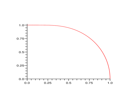
Figure 1: The Hagedorn temperature $\tilde{T}_{H}$ as function of $\tilde{h}$ for $\tilde{\lambda}=0$, with $\tilde{T}_{H}({\tilde{h}=0})=1/\log 2$.

We see from Fig. 1 that the Hagedorn temperature $\tilde{T}_{H}$ approaches zero for $\tilde{h}\rightarrow 1$. This confirms our upper bound on $\tilde{h}$ stating that $\tilde{h}\leq 1$, as found in Section 2.1, since planar $\mathcal{N}=4$ SYM in the decoupling limit (2.7) is only well-defined below the $\tilde{T}_{H}(\tilde{h})$ curve in Fig. 1. This has the consequence that we only reach $\tilde{h}=1$ when $\tilde{T}_{H}=0$.

Taking into account the corrections in $\tilde{\lambda}$, one can in principle plot the $\tilde{T}_{H}(\tilde{h})$ curve for small values of $\tilde{\lambda}$. From the first few corrections computed above, it is apparent that we still have that $\tilde{T}_{H}\rightarrow 0$ as $\tilde{h}\rightarrow 1$.

It is interesting to notice that the $\tilde{T}_{H}(\tilde{h})$ curve in Fig. 1 has a strong resemblance with the curves found in [18, 4] for $T_{H}$ as function of the chemical potentials in the full planar $\mathcal{N}=4$ SYM with zero ’t Hooft coupling. Thus it makes sense to regard $\tilde{h}$ as an effective chemical potential for the decoupled sector of $\mathcal{N}=4$ SYM in the limit (2.7), in the same sense that $\tilde{T}$ can be regarded as an effective temperature.

Hagedorn temperature from the pole of the partition function

As a consistency check, we compute here the Hagedorn temperature $\tilde{T}_{H}$ to order $\tilde{\lambda}$ directly from the partition function. This is a check on the consistency of the decoupling limit (2.7) and of the relation (2.19) between the Hagedorn temperature and the thermodynamics of the Heisenberg chain.

The Hagedorn temperature is given by the location of the first pole of the full partition function (2.4) in the planar limit $N=\infty$. Using this fact, the Hagedorn temperature can be calculated to first order in $\tilde{\lambda}$ by the technique introduced in [17] and extended to the case with chemical potentials in [4].

The tree-level Hagedorn temperature $\tilde{\beta}_{\textrm{H}}^{(0)}$ is obtained from the free partition function $Z^{(0)}$ which can be written as [17, 4]

$$\log Z^{(0)}(\tilde{\beta},\tilde{h})=-\sum_{k=1}^{\infty}\log\left(1-z(k\tilde{\beta},\tilde{h})\right).$$ (2.28)

The letter partition function $z$ with general chemical potentials was derived in [18, 4] and in the decoupling limit (2.7) it reduces to

$$z(\tilde{\beta},\tilde{h})=2e^{-\tilde{\beta}}\cosh(\tilde{\beta}\tilde{h}).$$ (2.29)

The pole is located where the letter partition function goes to one, as can be seen from equation (2.28). Note that it is the $k=1$ pole that we are interested in since this is the first pole that one encounters when raising the temperature. From Eq. (2.29) we then find that the tree-level Hagedorn inverse temperature $\tilde{\beta}^{(0)}_{\textrm{H}}$ is given by Eq. (2.24), as found from the Heisenberg chain through Eq. (2.19).

The one-loop correction to the inverse Hagedorn temperature is given by the residue at $\tilde{\beta}=\tilde{\beta}^{(0)}_{\textrm{H}}$ of the first order contribution to the single-trace partition function $\tilde{\lambda}Z^{(1)}_{\textrm{ST}}(\tilde{\beta},\tilde{h})$. This first-order contribution is known to be given by [17, 4]

$$Z^{(1)}_{\textrm{ST}}(\tilde{\beta},\tilde{h})=-\tilde{\beta}\sum_{L=1}^{\infty}\frac{\langle D_{2}(L\tilde{\beta},\tilde{h})\rangle}{1-z(L\tilde{\beta},\tilde{h})}+\textrm{(non-divergent $\langle PD_{2}\rangle$ terms)}.$$ (2.30)

The expectation value $\langle D_{2}(\tilde{\beta},\tilde{h})\rangle$ is a special case of the more general expectation value that was calculated in [4]. In our decoupling limit, it does not depend on $\tilde{h}$ and is simply given by

$$\langle D_{2}(\tilde{\beta},\tilde{h})\rangle=e^{-2\tilde{\beta}}.$$ (2.31)

The shift of the inverse Hagedorn temperature is therefore

$$\delta\tilde{\beta}_{\rm{H}}={\rm Res}_{\tilde{\beta}\to\tilde{\beta}^{(0)}_{\rm{H}}}\left(\frac{-\tilde{\beta}\tilde{\lambda}e^{-2\tilde{\beta}}}{1-z(\tilde{\beta},\tilde{h})}\right)$$ (2.32)

which precisely gives the one-loop contribution (2.25) to the Hagedorn temperature.

Thus, the more cumbersome method of computing the Hagedorn temperature to order $\tilde{\lambda}$ explicitly from the pole of the partition function gives the same result as computing it using Eq. (2.19). This illustrates how powerful the relation (2.19) is, also since it would be very hard to obtain higher order corrections in $\tilde{\lambda}$ directly from the pole of the partition function.

2.3 Spectrum with magnetic field for large $\tilde{\lambda}$ and large $L$

In this section we consider the spectrum of the single-trace operators of planar $\mathcal{N}=4$ SYM on $\mathbb{R}\times S^{3}$ in the decoupling limit (2.7) for large $\tilde{\lambda}$ and large $L$, $L$ being the length of the single-trace operators.

From Eqs. (2.14) and (2.15) it is clear that the effective Hamiltonian for the single-trace operators is $H=L+H_{XXX}$, with $H_{XXX}=\tilde{\lambda}D_{2}-2\tilde{h}S_{z}$. As explained above, $H_{XXX}$ is the Hamiltonian for the Heisenberg chain with coupling $\tilde{\lambda}$ and with an external magnetic field of magnitude $2\tilde{h}$. We see therefore that the large $\tilde{\lambda}$ regime corresponds to the low temperature regime $\tilde{\beta}\tilde{\lambda}\gg 1$ of the Heisenberg chain. We can therefore think of the spectrum for large $\tilde{\lambda}$ as the low energy spectrum for the Heisenberg chain.

We explain now first how to find the large $\tilde{\lambda}$ and large $L$ spectrum of single-trace operators by obtaining the low energy spectrum of the Heisenberg chain in a non-zero magnetic field $\tilde{h}$. After doing so, we discuss the physical difference from the spectrum for $\tilde{h}=0$ and we explain why this difference has important physical implications.

For $\tilde{h}>0$ the vacuum is $\mathop{{\rm Tr}}(Z^{L})$ and we get the excited states above the vacuum by inserting impurities in the form of $X$’s into the $Z$’s in the vacuum. Considering the case of $M$ impurities, each with momentum $p_{i}$, $i=1,...,M$, the spectrum of $H_{XXX}$ can be obtained using the Bethe ansatz technique together with the integrability of the Heisenberg chain [19]. The dispersion relation becomes

$$E=2\tilde{\lambda}\sum_{i=1}^{M}\sin^{2}\left(\frac{p_{i}}{2}\right)-\tilde{h}L+2\tilde{h}M$$ (2.33)

where $E$ is the eigenvalue of $H_{XXX}$. The two terms with $\tilde{h}$ arise from the $-2\tilde{h}S_{z}$ term in $H_{XXX}$. The $M$ momenta $p_{i}$ are determined from the algebraic Bethe equations

$$e^{ip_{k}L}=\prod_{j=1,j\neq k}^{M}S(p_{k},p_{j}),\quad S(p_{k},p_{j})=\frac{1+e^{i(p_{k}+p_{j})}-2e^{ip_{k}}}{1+e^{i(p_{k}+p_{j})}-2e^{ip_{j}}}$$ (2.34)

together with the following condition coming from the cyclicity of the trace

$$\sum_{i=1}^{M}p_{i}=0.$$ (2.35)

At this point we did not make any approximation. However, we now impose that we want the low energy spectrum in the thermodynamic limit $L\rightarrow\infty$. This spectrum consists of the magnon states, where each magnon corresponds to an impurity. In the low energy approximation, the momenta $p_{i}$ of the magnons are taken to be small. Also, we assume that $M\ll L$. From this we see that the Bethe equations (2.34) to leading order become $e^{ip_{k}L}=1$, $k=1,...,M$. The leading order solution for the momenta is therefore

$$p_{k}=\frac{2\pi n_{k}}{L}+\mathcal{O}(L^{-2})$$ (2.36)

where $n_{k}$ is an integer. Inserting this in the dispersion relation (2.33), we get the spectrum of the magnons

$$E=-\tilde{h}L+\frac{2\pi^{2}\tilde{\lambda}}{L^{2}}\sum_{k=1}^{M}n_{k}^{2}+2\tilde{h}M,\quad\sum_{k=1}^{M}n_{k}=0,$$ (2.37)

where the second equation is the cyclicity constraint (2.35). Defining now $M_{n}$ as the number of impurities/magnons at momentum level $n$, i.e. how many of the $n_{k}$’s are equal to $n$, we can write the spectrum as

$$E=-\tilde{h}L+\frac{2\pi^{2}\tilde{\lambda}}{L^{2}}\sum_{n\in\mathbb{Z}}n^{2}M_{n}+2\tilde{h}\sum_{n\in\mathbb{Z}}M_{n},\quad\sum_{n\in\mathbb{Z}}nM_{n}=0,$$ (2.38)

where we used that the total number of impurities is $M=\sum_{n\in\mathbb{Z}}M_{n}$.

Note that in the spectrum (2.38) we have in particular the mode $M_{0}$ that counts the number of impurities with zero momentum. If we consider the states that have only zero-momentum impurities, i.e. $M=M_{0}$, it is easily seen that they correspond to the totally symmetrized single-trace operators

$$\mathop{{\rm Tr}}(\mathrm{sym}(Z^{L-M}X^{M})).$$ (2.39)

Such operators are chiral primaries of $\mathcal{N}=4$ SYM, so we have that the vacuum $\mathop{{\rm Tr}}(Z^{L})$ and the zero modes (2.39) all correspond to chiral primaries.

Breaking of the degeneracy of the vacuum by the magnetic field

It is well known that there is a significant difference between the low energy spectrum of the ferromagnetic Heisenberg chain with or without the external magnetic field. With the magnetic field present, the spins prefer to be aligned in the direction of the field as the temperature goes to zero, but without $\tilde{h}$ there is no preferred direction and the vacuum is degenerate. We explain in the following how this manifests itself in our case.

We first review how the large $\tilde{\lambda}$ and large $L$ spectrum is found in the case of zero magnetic field $\tilde{h}=0$. This case, corresponding to planar $\mathcal{N}=4$ SYM on $\mathbb{R}\times S^{3}$ in the decoupling limit (1.1), is treated in Ref. [5]. There is a degeneracy of the vacuum into the $L+1$ different vacua

$$|S_{z}\rangle_{L}\sim\mathop{{\rm Tr}}(\mathrm{sym}(Z^{\frac{1}{2}L+S_{z}}X^{\frac{1}{2}L-S_{z}}))$$ (2.40)

with each vacuum labeled by $S_{z}$ since the vacuum is degenerate with respect to the total spin.

The low energy excitations above these vacua are magnons that can be constructed using a novel approach to the Bethe ansatz technique [5]. Starting from each vacuum $|S_{z}\rangle_{L}$, the magnons are made from impurities that correspond to acting with the operator $S_{z}$ on particular sites of the chain. In this way the total spin of the state does not change. The virtue of this method is that low energy excitations can be studied above any vacuum without running into finite size effects [5].

With the external magnetic field present, however, the situation has changed. The state $|S_{z}\rangle_{L}$ carries energy $-2\tilde{h}S_{z}$ and therefore $\mathop{{\rm Tr}}(Z^{L})$, which has $S_{z}=L/2$, becomes the unique vacuum and hence the $L+1$ fold degeneracy is removed. The method of [5] described above to build the low energy states on top of the degenerate vacuum will therefore no longer produce the correct spectrum. This can for example be seen by considering a state $|S_{z}\rangle_{L}$ with $S_{z}\leq 0$. The energy of such a state would at least be an energy $\tilde{h}L$ above the vacuum, which is outside the low energy regime that we are considering (since $L$ is large). Thus, we cannot simply perturb around the states obtained for $\tilde{h}=0$ in [5] to get the spectrum (2.38) for $\tilde{h}>0$. Therefore, the presence of the external magnetic field $\tilde{h}$ has a non-trivial physical effect, even if it is close to zero.

With the construction of the states where we insert $X$ as an impurity into the unique vacuum $\mathop{{\rm Tr}}(Z^{L})$, we find instead the low energy spectrum without running into problems with finite-size effects. We see also that the zero modes (2.39) in this case correspond to the broken vacuum states (2.40) for the $\tilde{h}=0$ case.

2.4 Hagedorn temperature for large $\tilde{\lambda}$

In this section we find the Hagedorn temperature $\tilde{T}_{H}$ of planar $\mathcal{N}=4$ SYM on $\mathbb{R}\times S^{3}$ in the decoupling limit (2.7) for large $\tilde{\lambda}$. The resulting temperature $\tilde{T}_{H}$ depends on both $\tilde{\lambda}$ and $\tilde{h}$. We compute $\tilde{T}_{H}$ by finding $V(\tilde{\beta})$ using the large $\tilde{\lambda}$ and large $L$ spectrum (2.38) derived in Section 2.3. The result that we get for the Hagedorn temperature will be matched to the Hagedorn temperature computed in string theory in Section 3.

From the spectrum (2.38) we get that the partition function for the Heisenberg chain for large $\tilde{\lambda}$ and large $L$ is given by

$${\mathop{{\rm Tr}}}_{L}\left(e^{-\tilde{\beta}H_{XXX}}\right)=\sum_{\{M_{n}\}}\int_{-1/2}^{1/2}du\,e^{-\tilde{\beta}\left(\frac{2\pi^{2}\tilde{\lambda}}{L^{2}}\sum_{n\in\mathbb{Z}}n^{2}M_{n}+2\tilde{h}\sum_{n\in\mathbb{Z}}M_{n}-\tilde{h}L\right)+2\pi iu\sum_{n\in\mathbb{Z}}nM_{n}}$$ (2.41)

where the range in the sum over $M_{n}$ is from zero to infinity and the cyclicity constraint in the spectrum (2.38) is imposed by introducing an integration over the variable $u$. After evaluating the sums over the $M_{n}$’s we have

$${\mathop{{\rm Tr}}}_{L}\left(e^{-\tilde{\beta}H_{XXX}}\right)=\int_{-1/2}^{1/2}du\,e^{\tilde{\beta}\tilde{h}L}\prod_{n=-\infty}^{\infty}\left[1-\exp\left(-\frac{2\pi^{2}\tilde{\beta}\tilde{\lambda}}{L^{2}}n^{2}-2\tilde{\beta}\tilde{h}+2\pi iun\right)\right]^{-1}.$$ (2.42)

In order to obtain $V(\tilde{\beta})$, we should extract from (2.42) the part that diverges like $\exp(\mbox{const.}\times L)$ for $L\rightarrow\infty$. It is possible to show that the leading divergent contribution comes from $u=0$ and that it is given by

$$\exp\left[\tilde{\beta}\tilde{h}L+L\sqrt{\frac{1}{2\pi\tilde{\beta}\tilde{\lambda}}}{\rm Li}_{\frac{3}{2}}\left(e^{-2\tilde{\beta}\tilde{h}}\right)\right]\ \ \mbox{for}\ \ L\rightarrow\infty$$ (2.43)

where ${\rm Li}_{n}(x)$ is the Polylogarithm function. Using this result we can determine the expression for the function $V(\tilde{\beta})$ in the large $\tilde{\lambda}$ limit which reads

$$V(\tilde{\beta})=\tilde{\beta}\tilde{h}+\sqrt{\frac{1}{2\pi\tilde{\beta}\tilde{\lambda}}}{\rm Li}_{\frac{3}{2}}\left(e^{-2\tilde{\beta}\tilde{h}}\right).\ \$$ (2.44)

This gives the thermodynamics of the Heisenberg chain with Hamiltonian (2.16) in the low temperature $\tilde{\beta}\tilde{\lambda}\ll 1$ and large $L$ limit. To the best of our knowledge, this is a new result for the magnetic Heisenberg chain.

Inserting now the result (2.44) in (2.19) we get the following equation for the Hagedorn temperature

$$\tilde{T}_{H}=\left[(1-\tilde{h})\sqrt{2\pi\tilde{\lambda}}\left({\rm Li}_{\frac{3}{2}}(e^{-2\tilde{h}/\tilde{T}_{H}})\right)^{-1}\right]^{2/3}.$$ (2.45)

Note that for $\tilde{h}=0$ we recover the result for the large $\tilde{\lambda}$ Hagedorn temperature recently obtained in [5].

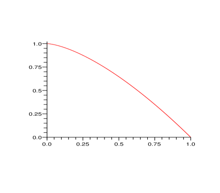
Figure 2: The Hagedorn temperature $\tilde{T}_{H}$ as function of $\tilde{h}$ for large $\tilde{\lambda}$. Here $\tilde{T}_{H}({\tilde{h}=0})=(2\pi)^{1/3}(\zeta(3/2))^{-2/3}\tilde{\lambda}^{1/3}$.

From Eq. (2.45) we see that the Hagedorn temperature goes like $\tilde{\lambda}^{1/3}$ to leading order so it is large for large $\tilde{\lambda}$. This means that $\tilde{h}/\tilde{T}_{H}$ is small since $0\leq\tilde{h}\leq 1$ and it makes sense therefore to expand the Polylogarithm function. This gives the following result for $\tilde{T}_{H}$ as a function of $\tilde{h}$ for large $\tilde{\lambda}$

$$\tilde{T}_{H}=\frac{(2\pi)^{\frac{1}{3}}(1-\tilde{h})^{\frac{2}{3}}}{\zeta(\frac{3}{2})^{\frac{2}{3}}}\tilde{\lambda}^{\frac{1}{3}}+\frac{4(2\pi)^{\frac{2}{3}}\sqrt{\tilde{h}}(1-\tilde{h})^{\frac{1}{3}}}{3\,\zeta(\frac{3}{2})^{\frac{4}{3}}}\,\tilde{\lambda}^{\frac{1}{6}}+\mathcal{O}(\tilde{\lambda}^{0}).$$ (2.46)

Note that at order $\tilde{\lambda}^{0}$ there are other corrections to the spectrum (2.38) that must be taken into account [5].

An interesting feature of (2.46) is that $\tilde{T}_{H}\rightarrow 0$ as $\tilde{h}\rightarrow 1$. This is the same as in the case of small $\tilde{\lambda}$, as found in Section 2.2. In Fig. 2 we have plotted the leading behavior of $\tilde{T}_{H}$ as a function of $\tilde{h}$ for large $\tilde{\lambda}$, i.e. the first term in (2.46). It is interesting to compare this curve to the one in Fig. 1 for $\tilde{\lambda}=0$. We expect that the shape of the curve will interpolate smoothly between the small and large $\tilde{\lambda}$ regimes.

3 String theory side: The magnetic pp-wave

In this section we consider the dual string theory version of the decoupling limit (2.7) of $\mathcal{N}=4$ SYM on $\mathbb{R}\times S^{3}$. We write down the limit in the microcanonical ensemble, which is appropriate for taking the limit on the string side. We then go on to find a Penrose limit which can give a pp-wave background compatible with the decoupling limit. After implementing the decoupling limit for the pp-wave, we match the spectrum and the Hagedorn temperature of weakly coupled strings to the corresponding quantities on the gauge theory side as obtained in Section 2.

3.1 Decoupling limit of strings on $\mbox{AdS}_{5}\times S^{5}$

In order to find the dual decoupling limit for strings on $\mbox{AdS}_{5}\times S^{5}$ we should first reformulate the decoupling limit (2.7) of thermal $\mathcal{N}=4$ SYM on $\mathbb{R}\times S^{3}$ as a decoupling limit that does not refer to temperature, i.e. a decoupling limit in the microcanonical ensemble. This can be done by analyzing the weight factor in the partition function (2.4) which we can write as

$$e^{-\beta(1-\Omega)J-\beta(D-J)+2\beta hS_{z}}.$$ (3.1)

With $h=0$ we can implement the decoupling limit (2.7) in the microcanonical ensemble by considering $\tilde{H}=(D-J)/\epsilon$ fixed and $\lambda/\epsilon$ fixed, and then taking $\epsilon\rightarrow 0$ [5]. However, we see here that the presence of the extra term means that we instead should rescale $D-J-2hS_{z}+hJ=D-J_{1}-(1-2h)J_{2}$, where we have added the term $hJ$ so that the vacuum has energy zero. It is important to remember that $h$ is also rescaled (see (2.7)), which is necessary to have the decoupling of the states in the $SU(2)$ sector. The decoupling limit of $\mathcal{N}=4$ SYM on $\mathbb{R}\times S^{3}$ in the microcanonical ensemble can thus be written as

$$\epsilon\rightarrow 0,\quad\tilde{H}\equiv\frac{D-J_{1}-(1-2h)J_{2}}{\epsilon}\ \mbox{fixed},\quad\tilde{\lambda}\equiv\frac{\lambda}{\epsilon}\ \mbox{fixed},\quad\tilde{h}\equiv\frac{h}{\epsilon}\ \mbox{fixed},\quad J_{i},N\ \mbox{fixed}.$$ (3.2)

This is the limit that we should translate to a decoupling limit of the dual string theory. Note that we have in the decoupling limit that

$$\tilde{H}=\tilde{h}J+\tilde{\lambda}D_{2}-2\tilde{h}S_{z}=\tilde{h}J+H_{XXX}$$ (3.3)

with $H_{XXX}$ defined as in (2.16).

On the string theory side, we are considering type IIB string theory on the $\mbox{AdS}_{5}\times S^{5}$ background given by the metric

$$ds^{2}=R^{2}\left[-\cosh^{2}\rho dt^{2}+d\rho^{2}+\sinh^{2}\rho d{\Omega^{\prime}_{3}}^{2}+d\theta^{2}+\sin^{2}\theta d\alpha^{2}+\cos^{2}\theta d\Omega_{3}^{2}\right]$$ (3.4)

and the five-form Ramond-Ramond field strength

$$F_{(5)}=2R^{4}(\cosh\rho\sinh^{3}\rho dtd\rho d\Omega_{3}^{\prime}+\sin\theta\cos^{3}\theta d\theta d\alpha d\Omega_{3}).$$ (3.5)

Here the radius $R$ is given by $R^{4}=4\pi g_{s}l_{s}^{4}N$ and $g_{\rm YM}^{2}=4\pi g_{s}$, where $g_{s}$ is the string coupling and $l_{s}$ is the string length. Note that $g_{\rm YM}$ and $N$ are the gauge coupling and rank of $SU(N)$ as defined in Section 2.1. With this, we see that we have the following dictionary between the gauge theory quantities $\lambda$ and $N$, and the string theory quantities $g_{s}$, $l_{s}$ and the AdS radius $R$

$$T_{\rm str}\equiv\frac{R^{2}}{4\pi l_{s}^{2}}=\frac{1}{2}\sqrt{\lambda},\quad g_{s}=\frac{\pi\lambda}{N}$$ (3.6)

where $T_{\rm str}$ is the string tension for a fundamental string in the $\mbox{AdS}_{5}\times S^{5}$ background (3.4)–(3.5).

In the following we write $E$ for the energy of the string. The energy $E$ for a string state is dual to the scaling dimension $D$ of a gauge theory state of $\mathcal{N}=4$ SYM on $\mathbb{R}\times S^{3}$ since we set the radius of the three-sphere to one. We furthermore write $J_{i}$, $i=1,2,3$, for the three angular momenta on the five-sphere dual to the three R-charges of $\mathcal{N}=4$ SYM, and we write $\Omega_{i}$, $i=1,2,3$, as the corresponding angular velocities, dual to the chemical potentials for the R-charges of $\mathcal{N}=4$ SYM.

We can now translate the decoupling limit (3.2) into the following limit of type IIB string theory on the $\mbox{AdS}_{5}\times S^{5}$ background (3.4)–(3.5)

$$\begin{array}[]{c}\displaystyle\epsilon\rightarrow 0,\quad\tilde{H}\equiv\frac{E-J_{1}-(1-2h)J_{2}}{\epsilon}\ \mbox{fixed},\quad\tilde{T}_{\rm str}\equiv\frac{T_{\rm str}}{\sqrt{\epsilon}}\ \mbox{fixed},\\[8.53581pt] \displaystyle\tilde{g}_{s}\equiv\frac{g_{s}}{\epsilon}\ \mbox{fixed},\quad\tilde{h}\equiv\frac{h}{\epsilon}\ \mbox{fixed},\quad J_{i}\ \mbox{fixed}.\end{array}$$ (3.7)

This limit closely resembles the decoupling limit of strings on $\mbox{AdS}_{5}\times S^{5}$ found in [5]. The only difference is the deformation caused by the $h$ parameter. This adds an extra term to the effective Hamiltonian $\tilde{H}$ for the strings. We also see that we get the following dictionary between the gauge theory and string theory quantities in the respective decoupling limits (3.2) and (3.7) [5]

$$\tilde{T}_{\rm str}=\frac{1}{2}\sqrt{\tilde{\lambda}},\quad\tilde{g}_{s}=\frac{\pi\tilde{\lambda}}{N}$$ (3.8)

which mirrors the AdS/CFT dictionary (3.6).

In order to fully justify that $\tilde{H}$ in (3.7) is the right expression for the effective Hamiltonian we should consider a thermal gas of strings in the $\mbox{AdS}_{5}\times S^{5}$ background (3.4)–(3.5). We can write the general partition function as

$$Z(\beta,\Omega_{i})=\mathop{{\rm Tr}}\left(e^{-\beta E+\beta\sum_{i=1}^{3}\Omega_{i}J_{i}}\right).$$ (3.9)

Putting $\Omega_{3}=0$ and writing $\Omega_{1}=\Omega+h$, $\Omega_{2}=\Omega-h$, $J=J_{1}+J_{2}$ and $S_{z}=(J_{1}-J_{2})/2$, as on the gauge theory side, we get

$$Z(\beta,\Omega,h)=\mathop{{\rm Tr}}\left(e^{-\beta E+\beta\Omega J+2\beta hS_{z}}\right)=\mathop{{\rm Tr}}\left(e^{-\beta[E-J_{1}-(1-2h)J_{2}]-\beta(1-\Omega-h)J}\right).$$ (3.10)

Taking now the limit (3.7) with

$$\epsilon=1-\Omega,\quad\tilde{T}\equiv\frac{T}{1-\Omega},$$ (3.11)

we see that the partition function (3.10) reduces to

$$Z(\tilde{\beta},\tilde{h})=\mathop{{\rm Tr}}\left\{\exp\left[-\tilde{\beta}\left((1-\tilde{h})J+\tilde{H}\right)\right]\right\}$$ (3.12)

where the trace is now over a reduced set of string theory states, corresponding to the decoupling of the $SU(2)$ sector on the gauge theory side. We see from this that the total Hamiltonian is $(1-\tilde{h})J+\tilde{H}$, thus for a fixed $J$ we can regard $\tilde{H}$ as the effective Hamiltonian. We note finally that $\tilde{h}\leq 1$ since otherwise the partition function (3.12) is not well-defined.

3.2 Finding the Penrose Limit

The goal of this section is to find a Penrose limit of $\mbox{AdS}_{5}\times S^{5}$ which gives a pp-wave background matching the large $\tilde{\lambda}$ spectrum and Hagedorn temperature found on the gauge theory side.

In the following we parameterize the three-sphere inside the five-sphere in (3.4) as

$$d\Omega_{3}^{2}=d\psi^{2}+\cos^{2}\psi d\chi^{2}+\sin^{2}\psi d\phi^{2}.$$ (3.13)

We define that $J_{1}=-i\partial_{\chi}$, $J_{2}=-i\partial_{\phi}$ and $J_{3}=-i\partial_{\alpha}$. From Section 3.1 we have that the effective Hamiltonian for which the vacuum state has zero energy is proportional to $E-J_{1}-(1-2h)J_{2}$. In accordance with previously found Penrose limits (see Appendix A for the BMN Penrose limit [11] and the Flat Direction Penrose limit [13]) this means that we should consider two new variables $\phi_{+}$ and $\phi_{-}$ defined in terms of the five-sphere coordinates $\chi$ and $\phi$ such that $J_{+}\equiv-i\partial_{\phi_{+}}=J_{1}+(1-2h)J_{2}$ since this gives that the Hamiltonian is proportional to $E-J_{+}$. Thus, we should require

$$\partial_{\phi_{+}}=\partial_{\chi}+(1-2h)\partial_{\phi}\,.$$ (3.14)

The most general linear relation between $\phi_{+}$, $\phi_{-}$ and $\chi$, $\phi$ obeying (3.14) is

$$\chi=\phi_{+}+c_{1}\phi_{-}\;,\quad\phi=(1-2h)\phi_{+}+c_{2}\phi_{-}\;.$$ (3.15)

We see from Appendix A that the BMN Penrose limit [11] corresponds to $h=1/2$, $c_{1}=0$ and $c_{2}=1$, while the Flat Direction Penrose limit [13] corresponds to $h=0$, $c_{1}=1$ and $c_{2}=-1$.

Define now, as in [5], the rescaled AdS radius $\tilde{R}$ by

$$\tilde{R}^{4}=\frac{R^{4}}{\epsilon}.$$ (3.16)

The rescaled radius $\tilde{R}$ is fixed in the decoupling limit (3.7). The light-cone coordinates are defined as

$$z^{+}=\frac{1}{2\mu}(t+\phi_{+}),\quad z^{-}=\frac{1}{2}\mu\tilde{R}^{2}(t-\phi_{+}),$$ (3.17)

where the mass parameter $\mu$ has been introduced for later convenience. The Penrose limit will then consist of taking the $\tilde{R}\rightarrow\infty$ limit. We now want to examine which choices of $c_{1}$ and $c_{2}$ can lead to a consistent Penrose limit.

Consider the following part of the the $\mbox{AdS}_{5}\times S^{5}$ metric (3.4)

$$\tilde{R}^{2}(-dt^{2}+\sin^{2}\psi d\phi^{2}+\cos^{2}\psi d\chi^{2}).$$ (3.18)

This is the only part of the metric where we can get $dz^{+}$ terms. Note that here and in the following we ignore the $\sqrt{\epsilon}$ factor in front of the metric since it will not be of importance for these considerations. Considering now only $(dz^{+})^{2}$ terms in (3.18), we get

$$-\mu^{2}\tilde{R}^{2}\left[1-(1-2h)\sin^{2}\psi-\cos^{2}\psi\right](dz^{+})^{2}.$$ (3.19)

Since this is of order $\tilde{R}^{2}$, we need that $(1-2h)\sin^{2}\psi+\cos^{2}\psi=1$ to leading order in $1/\tilde{R}$, in order to have a well-defined Penrose limit. However, this is equivalent to demanding that

$$h\sin^{2}\psi=0.$$ (3.20)

This is possible only if either $h=0$ or $\sin\psi=0$. Thus, if we want a background with $h>0$ we are bound to impose that $\sin\psi=0$ to leading order in $1/\tilde{R}$. On the other hand, with $h=0$ we can freely choose $\psi$, and for the Flat Direction Penrose limit (see Appendix A) this is used to choose $\psi=\pi/4$ to leading order. Therefore, any Penrose limit giving a background with $h>0$ will necessarily be disconnected from the Flat Direction limit no matter how small $h$ is. This can be understood as a geometric realization of the symmetry breaking caused by the magnetic field in the ferromagnetic Heisenberg spin chain as discussed in Section 2.3. For the spin chain it is well known that an arbitrarily small magnetic field can change the vacuum structure of the spin chain, and thereby also the low energy spectrum. In the context of Penrose limits of AdS${}_{5}\times S^{5}$, however, this is a new result.

Thus, we can conclude from the above that since we want a Penrose limit with $h>0$ we should have $\psi\rightarrow 0$ in the Penrose limit. Consider therefore the following part of the $\mbox{AdS}_{5}\times S^{5}$ metric (3.4) for $\rho=\theta=\psi=0$

$$\tilde{R}^{2}(-dt^{2}+d\chi^{2}).$$ (3.21)

In terms of $z^{\pm}$ and $\phi_{-}$, this metric is

$$-4dz^{+}dz^{-}+c_{1}^{2}\tilde{R}^{2}d\phi_{-}^{2}+2c_{1}\mu\tilde{R}^{2}dz^{+}d\phi_{-}-\frac{2c_{1}}{\mu}dz^{-}d\phi_{-}\,.$$ (3.22)

If $c_{1}\neq 0$, then the third terms means that we should have $\phi_{-}$ of order $1/\tilde{R}^{2}$ or of higher order. However, this has the consequence that $d\phi_{-}$ does not appear in any other part of the metric after the Penrose limit, which clearly is not consistent. Therefore, we can conclude that we should restrict ourselves to having $c_{1}=0$.

Now that $c_{1}=0$, we can choose our normalization for $\phi_{-}$ such that $c_{2}=1$. This is a useful choice since it means that $J_{-}\equiv-i\partial_{\phi_{-}}=J_{2}$. From our considerations we can therefore fix that

$$\chi=\phi_{+}\;,\quad\phi=(1-2h)\phi_{+}+\phi_{-}\;.$$ (3.23)

We can now write down the Penrose limit. Defining

$$r=\tilde{R}\rho,\quad\tilde{r}=\tilde{R}\theta,\quad\bar{r}=\tilde{R}\psi,$$ (3.24)

the Penrose limit is

$$\tilde{R}\rightarrow\infty,\quad z^{+},z^{-},r,\Omega_{3}^{\prime},\tilde{r},\alpha,\bar{r},\phi_{-}\ \mbox{fixed},$$ (3.25)

where the coordinates listed are defined in (3.4), (3.17), (3.23) and (3.24). The Penrose limit (3.25) of the $\mbox{AdS}_{5}\times S^{5}$ background (3.4)–(3.5) results in the following pp-wave background with metric

$$\begin{array}[]{rcl}\displaystyle\frac{1}{\sqrt{\epsilon}}ds^{2}&=&\displaystyle-4dz^{+}dz^{-}-\mu^{2}\left((1-(1-2h)^{2})\sum_{i=1}^{2}(z^{i})^{2}+\sum_{I=3}^{8}(z^{I})^{2}\right)(dz^{+})^{2}\\[11.38109pt] &&\displaystyle+\sum_{i=1}^{8}(dz^{i})^{2}+2\mu(1-2h)\left[z^{1}dz^{2}-z^{2}dz^{1}\right]dz^{+}\end{array}$$ (3.26)

and five-form field strength

$$\frac{1}{\epsilon}F_{(5)}=2\mu dz^{+}(dz^{1}dz^{2}dz^{3}dz^{4}+dz^{5}dz^{6}dz^{7}dz^{8}).$$ (3.27)

Here $\mu$ is the mass parameter introduced in (3.17). The coordinates $z^{1},z^{2}$ are defined by $z^{1}+iz^{2}=\bar{r}e^{i\phi_{-}}$, $z^{3},z^{4}$ are defined by $z^{3}+iz^{4}=\tilde{r}e^{i\alpha}$ and $z^{5},...,z^{8}$ are defined by $r^{2}=\sum_{i=5}^{8}(z^{i})^{2}$ and $dr^{2}+r^{2}d\Omega_{3}^{2}=\sum_{i=5}^{8}(dz^{i})^{2}$.

It is important to note that the Penrose limit (3.25) becomes the BMN Penrose limit (A.2) [11] if we set $h=1/2$. Moreover, as a consequence of this, the resulting pp-wave background (3.26)–(3.27) is seen to reduce to (A.3)–(A.4) for $h=1/2$.

Considering now the Penrose limit (3.25) in terms of the generators, we have the relations

$$H_{\rm lc}=\sqrt{\epsilon}\mu(E-J_{+}),\quad p^{+}=\frac{E+J_{+}}{2\mu R^{2}},$$ (3.28)

where $H_{\rm lc}$ is the light-cone Hamiltonian and $p^{+}$ is the light-cone momentum. It follows from these relations that the Penrose limit (3.25) is such that $J_{+}/\tilde{R}^{2}$ and $E-J_{+}$ are fixed in the limit $\tilde{R}\rightarrow\infty$. In particular, this means that $J_{+}=J_{1}+(1-2h)J_{2}\rightarrow\infty$. However, since $J_{-}=J_{2}$ and since we keep $\phi_{-}$ fixed, we have that $J_{2}$ is fixed in the Penrose limit (3.25). Therefore, in terms of $E$, $J_{1}$ and $J_{2}$, the Penrose limit (3.25) corresponds to taking the limit

$$\tilde{R}\rightarrow\infty,\quad J_{1}\rightarrow\infty,\quad\frac{J_{1}}{\tilde{R}^{2}}\ \mbox{fixed},\quad J_{2}\ \mbox{fixed},\quad E-J_{1}\ \mbox{fixed}.$$ (3.29)

We see that this is the same limit of the generators as that corresponding to the BMN Penrose limit [11]. We are thus considering the same set of string states in the Penrose limit (3.25) as in the BMN Penrose limit. This is contrary to the Flat Direction Penrose limit [13] which involves a different set of string states. We see therefore that even though $h$ can be arbitrarily close to zero, the Penrose limit concerns the same set of string states as for the BMN Penrose limit with $h=1/2$, despite the fact that the Flat Direction Penrose limit is the relevant one for $h=0$. This is another manifestation of the symmetry breaking caused by the magnetic field discussed in Section 2.3.

If we compare the background (3.26)–(3.27) to the pp-wave background (B.2)–(B.3) found in Appendix B by a constant rotation of the BMN pp-wave background (A.3)–(A.4) we see that (3.26)–(3.27) corresponds to the pp-wave background (B.2) for

$$\eta=1-2h,\quad C=0.$$ (3.30)

See Appendix B for a first quantization of type IIB string theory in the pp-wave background (B.2)–(B.3), leading to the string spectrum (B.2) with level-matching condition (B.19).

As we discuss in Appendix B there are two ways to think about the background (3.26)–(3.27). We can either think of it as the BMN pp-wave background rotated with a constant angular velocity in one of the two-planes. This makes sense since $h=(\Omega_{1}-\Omega_{2})/2$ and since $\Omega_{i}$ are angular velocities. Taking the limit $h\rightarrow 0$ as in (3.7) then means that we are approaching the critical angular velocity $\eta=1$.

Furthermore, as discussed in Section B.3, we can also think about the pp-wave background (3.26)–(3.27) as a magnetic pp-wave background, in the sense that the Hamiltonian for the background is equivalent to that of a particle in a constant magnetic field along with a harmonic oscillator potential. This is interesting since we precisely are turning on a magnetic field for the Heisenberg spin chain, and we can thus say that we have a correspondence between the magnetic Heisenberg spin chain and the magnetic pp-wave. However, the analogy is not perfect since the pp-wave can also be said to be magnetic for $h=0$.

3.3 Decoupling limit of the pp-wave and matching of spectra

We now implement the decoupling limit (3.7) for type IIB strings on $\mbox{AdS}_{5}\times S^{5}$ on the pp-wave background (3.26)–(3.27). Since we want to keep $p^{+}$ as given in (3.28) fixed in the decoupling limit we see that we need $\sqrt{\epsilon}\mu$ to be kept fixed, like in [5]. Therefore, we get that the decoupling limit for type IIB strings on the pp-wave background (3.26)–(3.27) is given by

$$\epsilon\rightarrow 0,\quad\tilde{\mu}\equiv\mu\sqrt{\epsilon}\ \mbox{fixed},\quad\tilde{H}_{\rm lc}\equiv\frac{H_{\rm lc}}{\epsilon}\ \mbox{fixed},\quad\tilde{h}\equiv\frac{h}{\epsilon}\ \mbox{fixed},\quad\tilde{g}_{s}\equiv\frac{g_{s}}{\epsilon}\ \mbox{fixed},\quad l_{s},\ p^{+}\ \mbox{fixed}.$$ (3.31)

We see that this limit reduces to the one of [5] for $\tilde{h}=0$. Clearly the limit (3.31) is a large $\mu$ limit of the magnetic pp-wave background (3.26)–(3.27). It is important to note here that we have the bound $0\leq\tilde{h}\leq 1$, where the upper bound is discussed above, and the lower bound comes from the fact that $h$ is required to be positive from the bound $|\eta|\leq 1$ and (3.30).

We obtain in Appendix B.2 the spectrum (B.2)–(B.19) for the pp-wave background (3.26)–(3.27), with $\eta$ given by (3.30). Taking then the decoupling limit (3.31), we get the reduced spectrum

$$\frac{1}{\tilde{\mu}}\tilde{H}_{\rm lc}=\frac{1}{2(\tilde{\mu}l_{s}^{2}p^{+})^{2}}\sum_{n\neq 0}n^{2}M_{n}+2\tilde{h}\sum_{n=-\infty}^{\infty}M_{n},\quad\quad\sum_{n\neq 0}nM_{n}=0,$$ (3.32)

where we also included the level matching condition. This is the spectrum for string theory on $\mbox{AdS}_{5}\times S^{5}$ in the decoupling limit (3.7) for large $\tilde{R}$ and large $J_{1}$. Note furthermore that from (3.28) we have

$$\tilde{\mu}l_{s}^{2}p^{+}=\frac{J_{1}}{4\pi\tilde{T}_{\rm str}}$$ (3.33)

so we are in a region with large $\tilde{T}_{\rm str}$ and $J_{1}$. It is interesting to observe from the spectrum (3.32) that the string theory effectively becomes one-dimensional in the sense that only the $M_{n}$ modes survive the limit (3.31).

We now translate our results for the string theory side to gauge theory, to examine the matching with the result for the gauge theory side in Section 2. From Eq. (3.8) we see that the Penrose limit (3.29) corresponds to the following region of the decoupled gauge theory

$$\tilde{\lambda}\rightarrow\infty,\quad J_{1}\rightarrow\infty,\quad\frac{\tilde{\lambda}}{J_{1}^{2}}\ \mbox{fixed},\quad J_{2}\ \mbox{fixed}.$$ (3.34)

Thus, we should match the spectrum (3.32) to the gauge theory spectrum for large $\tilde{\lambda}$ and large $L=J_{1}+J_{2}$, which is computed in Section 2.3. That $J_{2}$ is fixed in the Penrose corresponds to the fact that we are inserting $X$ as impurities in the ground state $\mathop{{\rm Tr}}(Z^{L})$ on the gauge theory side. Therefore, since $J_{2}$ is the number of impurities it is consistent with the gauge theory side that it is unaffected by the Penrose limit. Note also that this is consistent with our low energy approximation on the spin chain side in which we demand that the number of impurities is not large, i.e. $J_{2}\ll L$, since otherwise one runs into finite size effects.

Now that we have established that the Penrose limit regime (3.34) is in accordance with the low energy regime considered in Section 2.3, we are left with checking explicitly that the spectra (2.38) and (3.32) agree. To see this, we first note that one should identify $\tilde{H}$ in (3.2) and (3.7). Using then (3.3) we see that we should make the identification

$$\frac{1}{\tilde{\mu}}\tilde{H}_{\rm lc}=\tilde{h}L+H_{XXX}$$ (3.35)

between the string theory and the gauge theory/spin chain energies. Using then (3.33) and (3.8) we see that the spectrum (3.32) matches the spectrum (2.38) computed for planar $\mathcal{N}=4$ SYM on $\mathbb{R}\times S^{3}$ in the decoupling limit (2.7) for large $\tilde{\lambda}$ and large $L$. Note that as part of this matching we use that $J_{1}\simeq L$ since $J_{2}\ll L$.

3.4 Hagedorn temperature on the string side

In this section we compute the Hagedorn temperature for strings on the pp-wave background (3.26)–(3.27) in the decoupling limit (3.7), (3.31). The computation is done in two ways. First we compute the Hagedorn temperature using the reduced pp-wave spectrum (3.32) and subsequently we instead compute the Hagedorn temperature from the full pp-wave spectrum (B.2)–(B.19) and then we take the decoupling limit (3.31) on the result. We show that in both cases we get the same result, which, moreover, can be successfully matched with the Hagedorn temperature (2.45) computed on the gauge theory/spin-chain side. Note that on the gauge theory side we have weakly coupled $\mathcal{N}=4$ SYM.

The Hagedorn temperature of type IIB string theory on the maximally supersymmetric pp-wave background of [10] has previously been computed in [24, 25, 26, 27, 28, 29, 30, 31]. We begin by considering the multi-string partition function

$$\log Z(a,b,\mu,h)=\sum_{n=1}^{\infty}\frac{1}{n}\mbox{Tr}\left((-1)^{(n+1){\rm\bf F}}e^{-anH_{{\rm lc}}-bnp^{+}}\right)$$ (3.36)

where the trace is over single-string states with the spectrum (B.2)–(B.19), and ${\rm\bf F}$ is the space-time fermion number. The parameters $a$ and $b$ are introduced as the inverse temperature and chemical potential for strings on the pp-wave background (3.26)–(3.27).

We have seen that in the decoupling limit (3.31) most of the states decouple and the resulting pp-wave light-cone string spectrum is given by eq. (3.32). We see that only the term proportional to the bosonic modes $M_{n}$ contributes to the spectrum in the limit (3.31). We introduce therefore the “reduced” multi-string partition function

$$\log Z(\tilde{a},\tilde{b},\tilde{\mu},\tilde{h})=\sum_{n=1}^{\infty}\frac{1}{n}\mbox{Tr}\left(e^{-\tilde{a}n\tilde{H}_{{\rm lc}}-\tilde{b}np^{+}}\right)$$ (3.37)

where the trace is now taken over single-string states with spectrum (3.32) and $\tilde{a}$ and $\tilde{b}$ are the inverse temperature and chemical potential after the limit (3.31). The computation of the Hagedorn temperature then proceeds similarly to the one of Section 2.4. We obtain that the Hagedorn singularity is defined by the equation

$$\tilde{b}\sqrt{\tilde{a}}=l_{s}^{2}\sqrt{2\pi\tilde{\mu}}\,{\rm Li}_{3/2}\left(e^{-2\tilde{a}\tilde{\mu}\tilde{h}}\right)$$ (3.38)

where ${\rm Li}_{n}(x)$ is the Polylogaritm function. We now identify $\tilde{a}$ and $\tilde{b}$ in terms of the thermal partition function (3.12) for a thermal gas of strings in the $\mbox{AdS}_{5}\times S^{5}$ background in the decoupling limit (3.7). This is done using (3.28) and (3.31), along with (3.33) and the fact that $J_{1}\simeq J$. The result is

$$\tilde{a}=\frac{1}{\tilde{\mu}}\tilde{\beta},\quad\tilde{b}=\tilde{\beta}(1-\tilde{h})4\pi\tilde{\mu}l_{s}^{2}\tilde{T}_{\rm str}\,.$$ (3.39)

Substituting this in Eq. (3.38) we get the following equation for the Hagedorn temperature

$$\tilde{T}_{H}=\left[\sqrt{8\pi}(1-\tilde{h})\tilde{T}_{\rm str}\left({\rm Li}_{\frac{3}{2}}(e^{-2\tilde{h}/\tilde{T}_{H}})\right)^{-1}\right]^{2/3}.$$ (3.40)

This result is in agreement with the result of [5] for $\tilde{h}=0$. Note that from Section 3.3 we know that $\tilde{T}_{\rm str}$ is large and since $0\leq\tilde{h}\leq 1$ we get that $\tilde{h}/\tilde{T}_{H}\ll 1$. It is therefore sensible to expand the Polylogarithm function in (3.40).

We can now compare the equation for the Hagedorn temperature (3.40) to the gauge theory side. Using (3.8) it is easy to see that Eq. (3.40) matches with Eq. (2.45) on the gauge theory side. Thus, we have successfully matched the Hagedorn temperature as computed in planar $\mathcal{N}=4$ SYM on $\mathbb{R}\times S^{3}$ in the decoupling limit (2.7) for $\tilde{\lambda}\gg 1$ with the Hagedorn temperature computed in free string theory on $\mbox{AdS}_{5}\times S^{5}$ in the decoupling limit given by (3.7) and (3.11) for $\tilde{T}_{\rm str}\gg 1$.

The fact that we can match the Hagedorn temperature of gauge theory in the decoupling limit (2.7) and string theory in the decoupling limit given by (3.7) and (3.11) is a consequence of the fact that the spectra of the two theories match in the corresponding decoupling limits, as we verified in Section 3.3.

The Hagedorn/deconfinement temperature of planar $\mathcal{N}=4$ SYM on $\mathbb{R}\times S^{3}$ was conjectured to be dual to the Hagedorn temperature of string theory on AdS${}_{5}\times S^{5}$ in [6, 7, 8, 9]. Recently, the first successful matching of the Hagedorn temperature in AdS/CFT was done in [5]. The above matching of the Hagedorn temperature is an extension of that.

Decoupling limit of the Hagedorn singularity

As we remarked above, the matching of the gauge theory and string theory Hagedorn temperature can be seen as a consequence of the matching of the spectra (2.38) and (3.32). However, as a consistency check, we show in the following that the computation of the Hagedorn temperature for the string theory is consistent with the decoupling limit (3.31) that we take on the pp-wave spectrum (B.2)–(B.19). We do that by computing the Hagedorn temperature using the full pp-wave spectrum (B.2)–(B.19) and then taking the decoupling limit of the resulting equation for the Hagedorn singularity.

The starting point is now the partition function (3.36) and the computation of the Hagedorn singularity can be seen as a generalization of the computation in [28] to the case with an arbitrary parameter $\eta$ in the spectrum (B.2)–(B.19). We get the following equation for the Hagedorn singularity

$$b=4l_{s}^{2}\mu\sum_{p=1}^{\infty}\frac{1}{p}\left[3+\cosh(\eta\mu ap)-4(-1)^{p}\cosh(\frac{\eta\mu ap}{2})\right]K_{1}(\mu ap)$$ (3.41)

where $K_{\nu}(x)$ is the modified Bessel function of the second kind. This equation for the Hagedorn singularity contains as special cases both the Hagedorn singularity for the $\eta=1$ case corresponding to the Flat Direction pp-wave background (A.10)–(A.11) which is considered in [28, 5] and the $\eta=0$ case corresponding to the BMN pp-wave background (A.3)–(A.4) considered in [24, 25, 26, 27, 29].

The parameters $a$, $b$ and $\eta$ can be expressed in terms of quantities relating to strings on $\mbox{AdS}_{5}\times S^{5}$ as follows

$$a=\frac{\mu\tilde{\beta}}{\tilde{\mu}^{2}},\quad b=\tilde{\beta}(1-\tilde{h})4\pi\mu l_{s}^{2}T_{\rm str},\quad\eta=1-2h.$$ (3.42)

Now we take the limit (3.31) of the equation for the Hagedorn temperature and we use Eq. (3.42). It is easy to see that the only non-vanishing contribution in the limit (3.31) comes from the $M_{n}$ oscillators in the spectrum (B.2) while all the other terms vanish. This shows that in the decoupling limit those are precisely the only modes that survive. The result we get for the Hagedorn temperature is again (3.40).

4 Discussion and conclusions

In this paper we have modified the decoupling limit found in [4] to obtain an equivalence between planar $\mathcal{N}=4$ SYM on $\mathbb{R}\times S^{3}$ in the limit (2.7) and the ferromagnetic $XXX_{1/2}$ Heisenberg spin chain in an external magnetic field. The difference with the situation considered in [4, 5] is the extra parameter $\tilde{h}$ that plays the role of a magnetic field for the Heisenberg chain and can be regarded as an effective chemical potential for the gauge theory. The presence of the magnetic field $\tilde{h}$ breaks the the degeneracy of the vacuum and leaves a unique vacuum state ${\rm Tr}(Z^{L})$. It furthermore modifies the low energy spectrum in a non-trivial way such that it cannot be obtained for small $\tilde{h}$ as a perturbation of the case with zero magnetic field. This is an effect which is well known for spin systems.

As in the case of zero magnetic field analyzed in [4, 5] only the $SU(2)$ sector survives the limit (2.7). Moreover, the Hamiltonian truncates to $H=D_{0}+\tilde{\lambda}D_{2}-2\tilde{h}S_{z}$ which means that it consists of terms coming from the bare plus the one-loop part of the dilation operator. This has the consequence that we can study the resulting decoupled sector of $\mathcal{N}=4$ SYM for any value of the effective coupling $\tilde{\lambda}$. For small $\tilde{\lambda}$ we show that the first order term in $\tilde{\lambda}$ in the effective Hagedorn temperature $\tilde{T}_{H}$ comes from a one-loop correction in $\mathcal{N}=4$ SYM on $\mathbb{R}\times S^{3}$. Similarly, the $\tilde{\lambda}^{n}$ term comes from an $n$-loop correction. Therefore the large $\tilde{\lambda}$ regime can be seen as coming from the strong coupling regime of $\mathcal{N}=4$ SYM on $\mathbb{R}\times S^{3}$, even though we have that the ’t Hooft coupling $\lambda$ goes to zero in the decoupling limit (2.7). The truncation of the Hamiltonian thus has the consequence that we have a way to study aspects of the strong coupling regime of the gauge theory.

Following [5] we consider the decoupling limit (3.7) of strings on $\mbox{AdS}_{5}\times S^{5}$ which is dual to the gauge theory decoupling limit (2.7). We find a Penrose limit consistent with the decoupling limit (3.7). This leads us to consider type IIB strings propagating in the pp-wave background (3.26)–(3.27). The extra parameter $h$ on the gauge theory side coming from the difference between the chemical potentials emerges as a parameter in the pp-wave background, signifying an angular velocity in one of the two-planes. This new parameter allows us to get a pp-wave background that includes as special cases the BMN pp-wave background [10, 11] and the Flat Direction pp-wave background of [12, 13]. Indeed, the parameter $h$ measures the departure from the critical angular velocity giving the Flat Direction pp-wave background. Having $h>0$ breaks the explicit isometry of the flat direction and this is analogous to the breaking of the degeneracy of the vacuum states on the gauge-theory/spin-chain side.

The decoupling limit is implemented for the pp-wave background as the limit (3.31). Taking the decoupling limit of the pp-wave spectrum (B.2)–(B.19) we find the same spectrum as for large $\tilde{\lambda}$ and large $L$ on the gauge theory side. The matching of spectra is one of the main results of this paper. It is highly non-trivial since we are matching a spectrum computed for weak ’t Hooft coupling on the gauge theory side to a spectrum in free string theory. What makes us able to match the spectra is in part our ability to study the strong coupling regime of the gauge theory by having $\tilde{\lambda}\gg 1$, as described above. Another important ingredient is the fact that the pp-wave background is the maximally supersymmetric background pp-wave of [10] which is an exact background of type IIB string theory.

From the matching of the spectra it follows that we can match a limit of the Hagedorn temperature of string theory on the magnetic pp-wave background (3.26)–(3.27) to the Hagedorn temperature of weakly coupled planar $\mathcal{N}=4$ SYM on $\mathbb{R}\times S^{3}$ in the limit (2.7) for large $\tilde{\lambda}$ and for any value of the parameter $\tilde{h}$. This generalizes the matching of the Hagedorn temperature for $\tilde{h}=0$ in [5].

In conclusion, we have obtained a triality between planar $\mathcal{N}=4$ SYM on $\mathbb{R}\times S^{3}$ in the decoupling limit (2.7), the ferromagnetic $XXX_{1/2}$ Heisenberg spin chain coupled to an external magnetic field and free type IIB string theory on $\mbox{AdS}_{5}\times S^{5}$ in the limit (3.7). The difference with [5] is the extra parameter $\tilde{h}$. However, as in [5], we have that the Heisenberg chain with magnetic field is integrable which means that we have found a solvable sector of AdS/CFT.

One future direction which would be interesting to examine is to modify the $SU(2|3)$ decoupling limit of $\mathcal{N}=4$ SYM on $\mathbb{R}\times S^{3}$ found in [4] in a similar way as we modified the $SU(2)$ limit (1.1) in this paper. The resulting limit is

$$\begin{array}[]{c}\displaystyle\Omega\rightarrow 1,\quad\tilde{T}\equiv\frac{T}{1-\Omega}\ \mbox{fixed},\quad\tilde{h}_{1}\equiv\frac{h_{1}}{1-\Omega}\ \mbox{fixed},\quad\tilde{h}_{2}\equiv\frac{h_{2}}{1-\Omega}\ \mbox{fixed},\\[11.38109pt] \displaystyle\tilde{\lambda}\equiv\frac{\lambda}{1-\Omega}\ \mbox{fixed},\quad N\ \mbox{fixed},\end{array}$$ (4.1)

with $\Omega\equiv(\Omega_{1}+\Omega_{2}+\Omega_{3})/3$, $h_{1}\equiv(\Omega_{1}-\Omega_{2})/2$ and $h_{2}\equiv(\Omega_{2}-\Omega_{3})/2$. For $\tilde{h}_{1}=\tilde{h}_{2}=0$ this reduces to the $SU(2|3)$ limit of [4]. The full partition function of $\mathcal{N}=4$ SYM on $\mathbb{R}\times S^{3}$ in the limit (4.1) becomes

$$Z(\tilde{\beta},\tilde{h}_{1},\tilde{h}_{2})=\mathop{{\rm Tr}}\left[\exp\left(-\tilde{\beta}\left\{D_{0}+\tilde{\lambda}D_{2}-\frac{2}{3}\tilde{h}_{1}(2J_{1}+J_{2}+J_{3})-\frac{2}{3}\tilde{h}_{2}(J_{1}+J_{2}+2J_{3})\right\}\right)\right]$$ (4.2)

where the trace is over the $SU(2|3)$ sector of $\mathcal{N}=4$ SYM corresponding to the operators with $D_{0}=J_{1}+J_{2}+J_{3}$. Here $D_{2}$ is an extension of the $D_{2}$ operator given by Eq. (2.13) in the $SU(2)$ sector with the permutation operator now being the graded permutation operator. The interesting new feature in the $SU(2|3)$ sector is the presence of fermions. In order to find a string theory dual, it seems evident that one should consider a pp-wave background with two independent angular rotations in two orthogonal planes.

Another interesting direction that one could pursue is to take a further decoupling limit in the decoupled sector of $\mathcal{N}=4$ SYM on $\mathbb{R}\times S^{3}$ found in this paper. This is possible since we have introduced the extra parameter $\tilde{h}$ in the decoupled theory on the $SU(2)$. A particularly interesting limit is

$$\tilde{\lambda}\rightarrow\infty,\quad\tilde{h}\rightarrow 0,\quad\tilde{\lambda}(1-\tilde{h})^{2}\ \mbox{fixed}.$$ (4.3)

In this limit we are left only with the chiral primaries of the $SU(2)$ sector. However, the Hagedorn temperature $\tilde{T}_{H}$ remains finite, as is evident from (2.46). Thus, we have a phase transition in the supersymmetric sector of $\mathcal{N}=4$ SYM. This is similar in spirit to [33]. It would be interesting to explore this further also on the string theory side, and in particular to see if there is a connection with supersymmetric AdS black holes.

Finally, we note that there are several interesting recent works in the context of weakly coupled thermal $\mathcal{N}=4$ SYM on $\mathbb{R}\times S^{3}$ [34, 35, 36, 37] and related theories with less supersymmetry [38, 39, 40]. We believe that it could be interesting to combine studies of this kind with decoupling limits as presented in this paper, since this gives a way to explore the strongly coupled regime of the gauge theory and to relate gauge theory computations directly to the dual string theory.

Appendix A Penrose limits

In this appendix we write down the two Penrose limits of $\mbox{AdS}_{5}\times S^{5}$ background (3.4)–(3.5) that we compare our Penrose limit to in Section 3. Both limits give the maximally supersymmetric pp-wave background of [10] but in two different coordinate systems. Note that we use the rescaled AdS radius (3.16) in the limits.

BMN Penrose limit

We write here the BMN Penrose limit [11] (see also [41]). We define the coordinates

$$x^{-}=\frac{1}{2}\mu\tilde{R}^{2}(t-\chi),\quad x^{+}=\frac{1}{2\mu}(t+\chi),\quad r=\tilde{R}\rho,\quad\tilde{r}=\tilde{R}\theta,\quad\bar{r}=\tilde{R}\psi.$$ (A.1)

The BMN Penrose limit is then

$$\tilde{R}\rightarrow\infty,\quad x^{+},x^{-},r,\Omega_{3}^{\prime},\tilde{r},\alpha,\bar{r},\phi\ \mbox{fixed},$$ (A.2)

giving the pp-wave background of [10] with metric

$$\frac{1}{\sqrt{\epsilon}}ds^{2}=-4dx^{+}dx^{-}-\mu^{2}\sum_{i=1}^{8}x^{i}x^{i}(dz^{+})^{2}+\sum_{i=1}^{8}dx^{i}dx^{i}$$ (A.3)

and five-form field strength

$$\frac{1}{\epsilon}F_{(5)}=2\,\mu\,dx^{+}\left(dx^{1}dx^{2}dx^{3}dx^{4}+dx^{5}dx^{6}dx^{7}dx^{8}\right).$$ (A.4)

We denote this background as the BMN pp-wave background since it is the maximally supersymmetric pp-wave background of [10] in the coordinates used in [11]. The background (A.3)–(A.4) corresponds to (B.2) with $\eta=C=0$.

Flat Direction Penrose limit

We write here the Penrose limit of [13] giving the pp-wave background of [12] corresponding to the maximally supersymmetric pp-wave of [10] in a coordinate system in which we have explicitly a flat direction. This Penrose limit is denoted the Flat Direction Penrose limit in the main text.

Define $\phi_{+}$ and $\phi_{-}$ by

$$\chi=\phi_{+}+\phi_{-}\,,\quad\phi=\phi_{+}-\phi_{-}\,,$$ (A.5)

in terms of which the three-sphere metric (3.13) is

$$d\Omega_{3}^{2}=d\psi^{2}+d\phi_{+}^{2}+d\phi_{-}^{2}+2\cos(2\psi)d\phi_{+}d\phi_{-}\;.$$ (A.6)

We define the coordinates

$$z^{-}=\frac{1}{2}\mu\tilde{R}^{2}(t-\phi_{+}),\quad z^{+}=\frac{1}{2\mu}(t+\phi_{+}),$$ (A.7)

$$z^{1}=\tilde{R}\phi_{-},\quad z^{2}=\tilde{R}\left(\psi-\frac{\pi}{4}\right),\quad r=\tilde{R}\rho,\quad\tilde{r}=\tilde{R}\theta.$$ (A.8)

The Flat Direction Penrose limit is then (see also [5])

$$\tilde{R}\rightarrow\infty,\quad z^{+},z^{-},z^{1},z^{2},r,\Omega_{3}^{\prime},\tilde{r},\alpha\ \mbox{fixed}.$$ (A.9)

This gives the pp-wave background

$$\frac{1}{\sqrt{\epsilon}}ds^{2}=-4dz^{+}dz^{-}-\mu^{2}\sum_{I=3}^{8}(dz^{I})^{2}(dz^{+})^{2}+\sum_{i=1}^{8}dz^{i}dz^{i}-4\mu z^{2}dz^{1}dz^{+},$$ (A.10)

$$\frac{1}{\epsilon}F_{(5)}=2\,\mu\,dz^{+}\left(dz^{1}dz^{2}dz^{3}dz^{4}+dz^{5}dz^{6}dz^{7}dz^{8}\right).$$ (A.11)

This background corresponds to (B.2) with $\eta=C=1$.

Appendix B The magnetic pp-wave

In this appendix we find new pp-wave backgrounds by applying a time-dependent coordinate transformation to the maximally supersymmetric pp-wave background of [10] in the canonical coordinate system used in [10, 11], here denoted as the BMN pp-wave background. We find a two parameter family of pp-wave backgrounds that includes as special cases the BMN pp-wave background [10, 11] and the Flat Direction pp-wave background of [12, 13]. In addition, we get new magnetic pp-wave backgrounds. We call these backgrounds magnetic because the bosonic Hamiltonian has the same form as the Hamiltonian of a Newtonian point particle moving in a constant magnetic field.

B.1 Coordinate transformation for general $\eta$ and $C$

The BMN pp-wave background is given by (A.3)–(A.4). We consider here the coordinate transformation

$$\begin{gathered}x^{-}=z^{-}+\frac{\mu}{2}Cz^{1}z^{2},\\ \left(\begin{array}[]{c}x^{1}\\ x^{2}\end{array}\right)=\left(\begin{array}[]{cc}\cos(\eta\mu z^{+})&-\sin(\eta\mu z^{+})\\ \sin(\eta\mu z^{+})&\cos(\eta\mu z^{+})\end{array}\right)\left(\begin{array}[]{c}z^{1}\\ z^{2}\end{array}\right),\end{gathered}$$ (B.1)

leaving all other coordinates invariant. The metric (A.3) becomes

$$\frac{ds^{2}}{\sqrt{\epsilon}} = -4dz^{+}dz^{-}+dz^{i}dz^{i}-\mu^{2}(1-\eta^{2})\Big{(}(z^{1})^{2}+(z^{2})^{2}\Big{)}(dz^{+})^{2}-\mu^{2}\sum_{I=3}^{8}(dz^{I})^{2}(dz^{+})^{2}$$ (B.2)

$$-2\mu(C-\eta)z^{1}dz^{2}dz^{+}-2\mu(C+\eta)z^{2}dz^{1}dz^{+}$$

while the five-form field (A.4) is

$$\frac{1}{\epsilon}F_{(5)}=2\,\mu\,dz^{+}\left(dz^{1}dz^{2}dz^{3}dz^{4}+dz^{5}dz^{6}dz^{7}dz^{8}\right),$$ (B.3)

i.e. it is invariant under the coordinate transformation.

The parameters $\eta$ and $C$ can a priori take any value. Two special cases are $\eta=C=0$, which gives back the BMN pp-wave background (A.3)–(A.4), and $\eta=C=1$, which gives the Flat Direction pp-wave background (A.10)–(A.11). We will also be interested in the case with $0<\eta<1$ and $C=0$. This gives the new pp-wave backgrounds that we find in Section 3 to be dual to the Heisenberg spin-chain in an external magnetic field, when taking a limit with $\eta\rightarrow 1$.

B.2 String theory spectrum

In this section we derive the Hamiltonian and the spectrum of string theory on the magnetic pp-wave background (B.2)–(B.3). This is only a minor generalization of Section 3 in Ref. [13] and we will therefore be brief.

In the light-cone gauge, $Z^{+}=l_{s}^{2}p^{+}\tau$, the light-cone Lagrangian of the bosonic sigma-model is

$$\begin{array}[]{c}\displaystyle\frac{l_{s}^{2}p^{+}}{\sqrt{\epsilon}}\mathcal{L}_{\rm lc}=-\frac{1}{4\pi l_{s}^{2}}\left(\partial^{\alpha}Z^{i}\partial_{\alpha}Z^{i}+f^{2}(1-\eta^{2})\Big{(}(Z^{1})^{2}+(Z^{2})^{2}\Big{)}+f^{2}\sum_{I=3}^{8}(Z^{I})^{2}\right.\\[14.22636pt] \displaystyle\left.+2f(C-\eta)Z^{1}\dot{Z}^{2}+2f(C+\eta)Z^{2}\dot{Z}^{1}\right)\end{array}$$ (B.4)

where we have defined $f=\mu l_{s}^{2}p^{+}$. The conjugate momenta are

$$\Pi_{1}=\frac{\dot{Z}^{1}-f(C+\eta)Z^{2}}{2\pi l_{s}^{2}},\quad\Pi_{2}=\frac{\dot{Z}^{2}-f(C-\eta)Z^{1}}{2\pi l_{s}^{2}},\quad\Pi_{I}=\frac{\dot{Z}^{I}}{2\pi l_{s}^{2}},$$ (B.5)

giving the bosonic Hamiltonian

$$\frac{l_{s}^{2}p^{+}}{\sqrt{\epsilon}}H^{B}_{\rm lc}=\frac{1}{4\pi l_{s}^{2}}\int_{0}^{2\pi}d\sigma\left[\dot{Z}^{i}\dot{Z}^{i}+(Z^{i})^{\prime}(Z^{i})^{\prime}+f^{2}(1-\eta^{2})\big{(}(Z^{1})^{2}+(Z^{2})^{2}\big{)}+f^{2}\sum_{I=3}^{8}(Z^{I})^{2}\right].$$ (B.6)

Note that the parameter $C$ has dropped out of the Hamiltonian. That is because we have expressed it in terms of the velocities and not the true hamiltonian variables which are the conjugate momenta.

From the Lagrangian we find the equations of motion, expand the solutions in oscillator modes, and quantize in the canonical way. The bosonic Hamiltonian can then be written in terms of number operators as

$$\frac{l_{s}^{2}p^{+}}{\sqrt{\epsilon}}H^{\textrm{B}}_{\textrm{lc}}=\sum_{n=-\infty}^{\infty}\left((\omega_{n}+\eta f)N_{n}+(\omega_{n}-\eta f)M_{n}+\sum_{I=3}^{8}\omega_{n}N_{n}^{I}\right)$$ (B.7)

where

$$\omega_{n}=\sqrt{n^{2}+f^{2}},\quad\textrm{for all }n\in\mathbb{Z}.$$ (B.8)

If we consider the range of $\eta$, we find that for $\eta>1$ the mode $M_{0}$ has the spectrum

$$f(1-\eta)M_{0}$$ (B.9)

and therefore the Hamiltonian $H_{\rm lc}^{\rm B}$ can have arbitrarily large negative energies, signaling an instability. This suggests that having $\eta>1$ is not possible, and that $\eta=1$ is a critical value for $\eta$. Similarly, from the $N_{0}$ mode we get the condition $\eta\geq-1$. Thus, the physically acceptable range of $\eta$ is

$$-1\leq\eta\leq 1.$$ (B.10)

We find the fermionic part of the spectrum in exactly the same way as was done in Section 3.2 of [13]. Starting with $\theta^{A}$ as a Majorana-Weyl spinor with 16 non-vanishing components and $A=1,2$, we choose the light-cone gauge

$$Z^{+}=l_{s}^{2}\ p^{+}\tau,\qquad\Gamma^{\hat{+}}\theta^{A}=0.$$ (B.11)

The Green-Schwarz fermionic action is then given by [43]

$$\frac{l_{s}^{2}p^{+}}{\sqrt{\epsilon}}S^{\text{F}}_{\text{lc}}=\frac{i}{4\pi l_{s}^{2}}\int d\tau d\sigma\left[\left(\eta^{\alpha\beta}\delta_{AB}-\epsilon^{\alpha\beta}(\sigma_{3})_{AB}\right)\partial_{\alpha}Z^{+}\bar{\theta}^{A}\Gamma_{+}(\mathcal{D}_{\beta}\theta)^{B}\right]$$ (B.12)

and the generalized covariant derivative takes the form [43]

$$\mathcal{D}_{\beta}=\partial_{\beta}+\frac{1}{4}\partial_{\beta}Z^{+}\left(\omega_{+\hat{\rho}\hat{\sigma}}\Gamma^{\hat{\rho}\hat{\sigma}}-\frac{1}{2\cdot 5!}F_{\lambda\nu\rho\sigma\kappa}\Gamma^{\lambda\nu\rho\sigma\kappa}i\sigma_{2}\Gamma_{+}\right).$$ (B.13)

In order to proceed, we need to find all the relevant components of the spin connection $\omega_{\mu\hat{a}\hat{b}}$. We put a hat on flat indices in the tangent space to distinguish them from the curved indices in the spacetime. For our purposes here it is enough to find the components where the curved index is $+$. It turns out that the only relevant components are

$$\omega_{+\hat{1}\hat{2}}=-\eta\mu,\quad\omega_{+\hat{2}\hat{1}}=\eta\mu.$$ (B.14)

The other components either vanish, like $\omega_{+\hat{I}\hat{J}}=0$, or are contracted with $\Gamma^{\hat{+}}$ in the covariant derivative and are thus killed in the light-cone gauge, like $\omega_{+\hat{+}\hat{I}}=-\mu^{2}z^{I}$.

Following the same steps as in the paper [13] (and using the same notation), we arrive at the fermionic light-cone action

$$\frac{l_{s}^{2}p^{+}}{\sqrt{\epsilon}}S^{\textrm{F}}_{\textrm{lc}}=\frac{i}{2\pi}\int d\tau d\sigma\left[S^{1}\left(\partial_{+}-\frac{\eta f}{2}\gamma^{12}\right)S^{1}+S^{2}\left(\partial_{-}-\frac{\eta f}{2}\gamma^{12}\right)S^{2}-2fS^{1}\Pi S^{2}\right]$$ (B.15)

where $\partial_{\pm}=\partial_{\tau}\pm\partial_{\sigma}\,$ and $\Pi=\gamma^{1234}$. Note that there are two “sources” of terms involving $f=\mu l_{s}^{2}p^{+}$. The $S^{A}\eta f\gamma^{12}S^{A}$ terms come from the spin connection (B.14) and therefore the $f$ in [13] is replaced by $\eta f$ here, while the $2fS^{1}\Pi S^{2}$ term comes from the five-form field and thus does not contain any $\eta$.

Again, following the same steps as in Sections 3.2–3.3 of [13], we find that the fermionic part of the Hamiltonian is given by

$$\frac{l_{s}^{2}p^{+}}{\sqrt{\epsilon}}H_{\textrm{lc}}^{\textrm{F}} =\sum_{n=-\infty}^{+\infty}S^{\dagger}_{n}\left(\omega_{n}+i\frac{\eta f}{2}\gamma^{12}\right)S_{n}$$ (B.16)

$$=\sum_{n=-\infty}^{+\infty}\left[\sum_{b=1}^{4}\left(\omega_{n}-\frac{\eta f}{2}\right)F_{n}^{(b)}+\sum_{b=5}^{8}\left(\omega_{n}+\frac{\eta f}{2}\right)F_{n}^{(b)}\right].$$ (B.17)

The full Hamiltonian of quantized strings on the magnetic pp-wave in light-cone gauge is therefore

$$\frac{l_{s}^{2}p^{+}}{\sqrt{\epsilon}}H_{\textrm{lc}} =\sum_{n=-\infty}^{+\infty}\left((\omega_{n}+\eta f)N_{n}+(\omega_{n}-\eta f)M_{n}+\sum_{I=3}^{8}\omega_{n}N_{n}^{I}\right)$$

$$+\sum_{n=-\infty}^{+\infty}\left(\sum_{b=1}^{4}\left(\omega_{n}-\frac{\eta f}{2}\right)F_{n}^{(b)}+\sum_{b=5}^{8}\left(\omega_{n}+\frac{\eta f}{2}\right)F_{n}^{(b)}\right)$$ (B.18)

with the level matching condition

$$\sum_{n=-\infty}^{+\infty}n\left(N_{n}+M_{n}+\sum_{I=3}^{8}N_{n}^{I}+\sum_{b=1}^{8}F_{n}^{(b)}\right)=0.$$ (B.19)

B.3 Physical interpretation

We can compare the bosonic Hamiltonian of the magnetic pp-wave in equation (B.6) to Newtonian physics of a charged particle moving in a constant magnetic field. We will see that the parameter $\eta$ corresponds to the strength of the magnetic field while $C$ is a gauge choice.

To be more precise, let the particle move in the $(z^{1},z^{2})$ plane with a constant magnetic field $\vec{B}=B\vec{e}_{3}$ perpendicular to the plane. The particle is furthermore connected to the origin with a spring of spring constant $k$. We can take the vector potential to be

$$\vec{A}=\frac{1}{2}\vec{B}\times\vec{z}=\frac{B}{2}\left(-z^{2},z^{1},0\right)^{T}$$ (B.20)

but we are also free to add any $\vec{\nabla}\phi$ to the vector potential since that only amounts to choosing a different gauge. Let’s take $\phi=\gamma z^{1}z^{2}$ so that

$$\vec{\nabla}\phi=\gamma\left(z^{2},z^{1},0\right)^{T}.$$ (B.21)

To find the Hamiltonian of this system, we start with the Hamiltonian of an uncharged particle and simply replace $\vec{p}$ with $\vec{p}+\vec{A}$. This gives

$$H =\frac{1}{2m}(\vec{p}+\vec{A})^{2}+\frac{1}{2}k\vec{z}^{2}$$ (B.22)

$$=\frac{1}{2m}\left\{\left(p_{1}+(\gamma-B/2)z^{2}\right)^{2}+\left(p_{2}+(\gamma+B/2)z^{1}\right)^{2}\right\}+\frac{1}{2}k\left((z^{1})^{2}+(z^{2})^{2}\right).$$ (B.23)

This Hamiltonian should be compared to the $Z^{1}$ and $Z^{2}$ part of the bosonic Hamiltonian (B.6) with the velocities $\dot{Z}^{i}$ replaced by the conjugate momenta $\Pi_{i}$ from Eq. (B.5). Let’s set $2\pi\ell_{s}^{2}=m=1$ for now. The relevant part of the bosonic Hamiltonian is then

$$\frac{1}{2}\int_{0}^{2\pi}d\sigma\left[\left(\Pi_{1}+f(C+\eta)Z^{2}\right)^{2}+\left(\Pi_{2}+f(C-\eta)Z^{1}\right)^{2}+f^{2}(1-\eta^{2})\big{(}(Z^{1})^{2}+(Z^{2})^{2}\big{)}\right].$$ (B.24)

Comparing this to Eq. (B.23) we find the following dictionary

$$-\frac{B}{2}\leftrightarrow f\eta,\qquad\gamma\leftrightarrow fC,\qquad k\leftrightarrow f^{2}(1-\eta^{2}).$$ (B.25)

This shows that the parameter $\eta$ corresponds to the strength of the magnetic field and that $C$ is a gauge choice for the vector potential.

The BMN background corresponds to having no magnetic field while in the Flat Direction background, the gauge $C=\eta$ was chosen to eliminate all dependence of $Z^{1}$ from the Hamiltonian.

References

- [1] J. Maldacena, “The large N limit of superconformal field theories and supergravity,” Adv. Theor. Math. Phys. 2 (1998) 231–252, hep-th/9711200.
- [2] S. S. Gubser, I. R. Klebanov, and A. M. Polyakov, “Gauge theory correlators from noncritical string theory,” Phys. Lett. B428 (1998) 105, hep-th/9802109.
- [3] E. Witten, “Anti-de Sitter space and holography,” Adv. Theor. Math. Phys. 2 (1998) 253, hep-th/9802150.
- [4] T. Harmark and M. Orselli, “Quantum mechanical sectors in thermal super Yang-Mills on ,” Nucl. Phys. B757 (2006) 117–145, hep-th/0605234.
- [5] T. Harmark and M. Orselli, “Matching the Hagedorn temperature in AdS/CFT,” Phys. Rev. D74 (2006) 126009, hep-th/0608115.
- [6] E. Witten, “Anti-de Sitter space, thermal phase transition, and confinement in gauge theories,” Adv. Theor. Math. Phys. 2 (1998) 505, hep-th/9803131.
- [7] B. Sundborg, “The Hagedorn transition, deconfinement and SYM theory,” Nucl. Phys. B573 (2000) 349–363, hep-th/9908001.
- [8] A. M. Polyakov, “Gauge fields and space-time,” Int. J. Mod. Phys. A17S1 (2002) 119–136, hep-th/0110196.
- [9] O. Aharony, J. Marsano, S. Minwalla, K. Papadodimas, and M. Van Raamsdonk, “The Hagedorn/deconfinement phase transition in weakly coupled large N gauge theories,” hep-th/0310285.
- [10] M. Blau, J. Figueroa-O’Farrill, C. Hull, and G. Papadopoulos, “A new maximally supersymmetric background of IIB superstring theory,” JHEP 01 (2002) 047, hep-th/0110242.
- [11] D. Berenstein, J. M. Maldacena, and H. Nastase, “Strings in flat space and pp waves from super Yang Mills,” JHEP 04 (2002) 013, hep-th/0202021.
- [12] J. Michelson, “(twisted) toroidal compactification of pp-waves,” Phys. Rev. D66 (2002) 066002, hep-th/0203140.
- [13] M. Bertolini, J. de Boer, T. Harmark, E. Imeroni, and N. A. Obers, “Gauge theory description of compactified pp-waves,” JHEP 01 (2003) 016, hep-th/0209201.
- [14] N. Beisert, C. Kristjansen, and M. Staudacher, “The dilatation operator of super Yang-Mills theory,” Nucl. Phys. B664 (2003) 131–184, hep-th/0303060.
- [15] N. Beisert, “The dilatation operator of super Yang-Mills theory and integrability,” Phys. Rept. 405 (2005) 1–202, hep-th/0407277.
- [16] J. A. Minahan and K. Zarembo, “The Bethe-ansatz for super Yang-Mills,” JHEP 03 (2003) 013, hep-th/0212208.
- [17] M. Spradlin and A. Volovich, “A pendant for Polya: The one-loop partition function of SYM on ,” Nucl. Phys. B711 (2005) 199–230, hep-th/0408178.
- [18] D. Yamada and L. G. Yaffe, “Phase diagram of super-Yang-Mills theory with R-symmetry chemical potentials,” JHEP 09 (2006) 027, hep-th/0602074.
- [19] M. Takahashi, Thermodynamics of One-Dimensional Solvable Models. Cambridge University Press, 1999.
- [20] M. Takahashi, “Simplification of thermodynamic Bethe-ansatz equations,” cond-mat/0010486.
- [21] M. Takahashi, M. Shiroishi, and A. Klümper, “Equivalence of TBA and QTM,” J. Phys. A: Math. Gen. 34 (2001) L187–L194.
- [22] M. Shiroishi and M. Takahashi, “Integral equation generates high-temperature expansion of the Heisenberg chain,” Phys. Rev. Lett. 89 (2002), no. 11, 117201.
- [23] T. Harmark and N. A. Obers, “Thermodynamics of spinning branes and their dual field theories,” JHEP 01 (2000) 008, hep-th/9910036.
- [24] L. A. Pando Zayas and D. Vaman, “Strings in RR plane wave background at finite temperature,” Phys. Rev. D67 (2003) 106006, hep-th/0208066.
- [25] B. R. Greene, K. Schalm, and G. Shiu, “On the Hagedorn behaviour of pp-wave strings and SYM theory at finite R-charge density,” Nucl. Phys. B652 (2003) 105–126, hep-th/0208163.
- [26] Y. Sugawara, “Thermal amplitudes in DLCQ superstrings on pp-waves,” Nucl. Phys. B650 (2003) 75–113, hep-th/0209145.
- [27] R. C. Brower, D. A. Lowe, and C.-I. Tan, “Hagedorn transition for strings on pp-waves and tori with chemical potentials,” Nucl. Phys. B652 (2003) 127–141, hep-th/0211201.
- [28] Y. Sugawara, “Thermal partition function of superstring on compactified pp-wave,” Nucl. Phys. B661 (2003) 191–208, hep-th/0301035.
- [29] G. Grignani, M. Orselli, G. W. Semenoff, and D. Trancanelli, “The superstring Hagedorn temperature in a pp-wave background,” JHEP 06 (2003) 006, hep-th/0301186.
- [30] S.-j. Hyun, J.-D. Park, and S.-H. Yi, “Thermodynamic behavior of IIA string theory on a pp-wave,” JHEP 11 (2003) 006, hep-th/0304239.
- [31] F. Bigazzi and A. L. Cotrone, “On zero-point energy, stability and Hagedorn behavior of type IIB strings on pp-waves,” JHEP 08 (2003) 052, hep-th/0306102.
- [32] N. Deo, S. Jain, and C.-I. Tan, “String statistical mechanics above Hagedorn energy density,” Phys. Rev. D40 (1989) 2626. R. C. Brower, J. McGreevy, and C. I. Tan, “Stringy model for QCD at finite density and generalized Hagedorn temperature,” hep-ph/9907258. G. Grignani, M. Orselli, and G. W. Semenoff, “Matrix strings in a B-field,” JHEP 07 (2001) 004, hep-th/0104112. G. Grignani, M. Orselli, and G. W. Semenoff, “The target space dependence of the Hagedorn temperature,” JHEP 11 (2001) 058, hep-th/0110152. G. De Risi, G. Grignani, and M. Orselli, “Space / time noncommutativity in string theories without background electric field,” JHEP 12 (2002) 031, hep-th/0211056.
- [33] P. J. Silva, “Phase transitions and statistical mechanics for BPS black holes in AdS/CFT,” JHEP 03 (2007) 015, hep-th/0610163.
- [34] L. Alvarez-Gaume, P. Basu, M. Marino, and S. R. Wadia, “Blackhole / string transition for the small Schwarzschild blackhole of and critical unitary matrix models,” Eur. Phys. J. C48 (2006) 647–665, hep-th/0605041.
- [35] T. Hollowood, S. P. Kumar, and A. Naqvi, “Instabilities of the small black hole: A view from SYM,” JHEP 01 (2007) 001, hep-th/0607111.
- [36] S. A. Hartnoll and S. P. Kumar, “Thermal SYM theory as a 2D Coulomb gas,” Phys. Rev. D76 (2007) 026005, hep-th/0610103.
- [37] G. Festuccia and H. Liu, “The arrow of time, black holes, and quantum mixing of large N Yang-Mills theories,” hep-th/0611098.
- [38] A. Karch and A. O’Bannon, “Chiral transition of super Yang-Mills with flavor on a 3-sphere,” Phys. Rev. D74 (2006) 085033, hep-th/0605120.
- [39] T. J. Hollowood and A. Naqvi, “Phase transitions of orientifold gauge theories at large N in finite volume,” JHEP 04 (2007) 087, hep-th/0609203.
- [40] Y. Hikida, “Phase transitions of large N orbifold gauge theories,” JHEP 12 (2006) 042, hep-th/0610119.
- [41] M. Blau, J. Figueroa-O’Farrill, C. Hull, and G. Papadopoulos, “Penrose limits and maximal supersymmetry,” Class. Quant. Grav. 19 (2002) L87–L95, hep-th/0201081.
- [42] J. Gomis and H. Ooguri, “Penrose limit of gauge theories,” Nucl. Phys. B635 (2002) 106–126, hep-th/0202157.
- [43] R. R. Metsaev and A. A. Tseytlin, “Exactly solvable model of superstring in plane wave Ramond-Ramond background,” Phys. Rev. D65 (2002) 126004, hep-th/0202109.