hep-th/0611229

Bicocca-FT-06-18

LPTENS-06/54

SISSA 65/2006/EP

Counting BPS Baryonic Operators in CFTs

with Sasaki-Einstein duals

Agostino Butti ^a, Davide Forcella ^b, Alberto Zaffaroni ^c

^a Laboratoire de Physique Théorique de l’École Normale Supérieure
24, rue Lhomond, 75321 Paris Cedex 05, France

^b International School for Advanced Studies (SISSA / ISAS)
via Beirut 2, I-34014, Trieste, Italy

^c Università di Milano-Bicocca and INFN, sezione di Milano-Bicocca
P.zza della Scienza, 3; I-20126 Milano, Italy

We study supersymmetric D3 brane configurations wrapping internal cycles of type II backgrounds $AdS_{5}\times H$ for a generic Sasaki-Einstein manifold H. These configurations correspond to BPS baryonic operators in the dual quiver gauge theory. In each sector with given baryonic charge, we write explicit partition functions counting all the BPS operators according to their flavor and R-charge. We also show how to extract geometrical information about H from the partition functions; in particular, we give general formulae for computing volumes of three cycles in H.

 agostino.butti@lpt.ens.fr
forcella@sissa.it
alberto.zaffaroni@mib.infn.it

1 Introduction

The study of $BPS$ states in quantum field theory and in string theory is clearly a very important topic. These states are generically protected against quantum corrections and contain information regarding the strong coupling behaviour of supersymmetric field theories and superstring theories. In the past years they were especially important in the study of strong weak dualities, like the AdS/CFT conjecture [1] which gives a connection between the $BPS$ operators in conformal field theories and $BPS$ states in string theory.

In this paper we discuss the set of one half $BPS$ states in string theory realized as $D3$ branes wrapped on (generically non trivial) three cycles in the supergravity background $AdS_{5}\times H$, where $H$ is a Sasaki-Einstein manifold [2, 3]. These states are holographically dual to baryonic $BPS$ operators in $\mathcal{N}=1$ four dimensional $CFT$s [4], which are quiver gauge theories.

Recently, there has been renewed interest in generalizing the $AdS/CFT$ correspondence to generic Sasaki-Einstein manifolds $H$. This interest has been initially motivated by the discovery of new infinite classes of non compact $CY$ metrics [5, 6, 7, 8] and the construction of their dual $\mathcal{N}=1$ supersymmetric $CFT$ [9, 10, 11, 12] . As a result of this line of investigation, we now have a well defined correspondence between toric CY and dual quiver gauge theories [10, 12, 14, 16, 15, 17, 18, 19, 20, 21, 22]. The non toric case is still less understood: there exist studies on generalized conifolds [23, 24], del Pezzo series [25, 26, 27], and more recently there was a proposal to construct new non toric examples [28].

There has been some parallel interest in counting $BPS$ states in the $CFT$s dual to CY singularities [29, 30, 32, 31, 33, 34]. The partition function counting mesonic $BPS$ gauge invariant operators according to their flavor quantum numbers contains a lot of information regarding the geometry of the $CY$ [33, 35], including the algebraic equations of the singularity. Quite interestingly, it also provides a formula for the volume of $H$ [35]. This geometrical information has a direct counterpart in field theory, since, according to the $AdS/CFT$ correspondence, the volume of the total space and of the three cycles are duals to the central charge and the $R$ charges of the baryonic operators respectively [4, 37].

The existing countings focus on the mesonic gauge invariant sector of the $CFT$. Geometrically this corresponds to consider giant graviton configurations [36] corresponding to $BPS$ $D3$ branes wrapped on trivial three cycles in $H$. In this paper we push this investigation further and we analyze the baryonic $BPS$ operators, corresponding to $D3$ branes wrapped on non trivial three cycles inside $H$. We succeed in counting $BPS$ states charged under the baryonic charges of the field theory and we write explicit partition functions at fixed baryonic charge. We investigate in details their geometrical properties. In particular we will show how to extract from the baryonic partition functions a formula for the volume of the three cycles inside $H$. We will mostly concentrate on the toric case but our procedure seems adaptable to the non toric case as well.

The paper is organized as follows. In Section 2 we review some basic elements of toric geometry. In Section 3 we formulate the general problem of describing and quantizing the $BPS$ $D3$ brane configurations. We will use homomorphic surfaces to parameterize the supersymmetric $BPS$ configurations of $D3$ brane wrapped in $H$, following results in [38, 39] . In the case where $X$ is a toric variety we have globally defined homogeneous coordinates $x_{i}$ which are charged under the baryonic charges of the theory and which we can use to parametrize these surfaces. We will quantize configurations of D3 branes wrapped on these surfaces and we will find the Hilbert space of $BPS$ states using a prescription found by Beasley [39]. The complete $BPS$ Hilbert space factorizes in sectors with definite baryonic charges. Using toric geometry tools, we can assign to each sector a convex polyhedron $P$. The BPS operators in a given sector are in one-to-one correspondence with symmetrized products of N (number of colors) integer points in $P$. In Section 4 we discuss the assignment of charges and we set the general counting problem. In Section 5 we make some comparison with the field theory side. In Section 6, we will write a partition function $Z_{D}$ counting the integer points in $P_{D}$ and a partition function $Z_{D,N}$ counting the integer points in the symmetric product of $P_{D}$. From $Z_{D}$, taking a suitable limit, we will be able to compute the volume of the three cycles in $H$, as described in Section 7. Although we mainly focus on the toric case we propose a general formula for the computation of the volume of the three cycles valid for every type of conical $CY$ singularity.

From the knowledge of $Z_{D,N}$ we can reconstruct the complete partition function for the chiral ring of quiver gauge theories. This is a quite hard problem in field theory, since we need to count gauge invariant operators modulo F-term relations and to take into account the finite number of colors $N$ which induces relations among traces and determinants. The geometrical computation of $Z_{D,N}$ should allow to by-pass these problems. In this paper we will mainly focus on the geometrical properties of the partition functions $Z_{D}$, although some preliminary comparison with the dual gauge theory is made in Section 5. In forthcoming papers, we will show how to compute the complete partition function for selected examples and how to compare with field theory expectations [42].

2 A short review of toric geometry

In this section we summarize some basic topics of toric geometry; in particular we review divisors and line bundles on toric varieties that will be very useful for the complete understanding of the paper. Very useful references on toric geometry are [44, 43].

A toric variety $V_{\Sigma}$ is defined by a fan $\Sigma$: a collection of strongly convex rational polyhedral cones in the real vector space $N_{\mathbb{R}}=N\otimes_{\mathbb{Z}}\mathbb{R}$ ($N$ is an $n$ dimensional lattice $N\simeq\mathbb{Z}^{n}$). Some examples are presented in Figure 1.

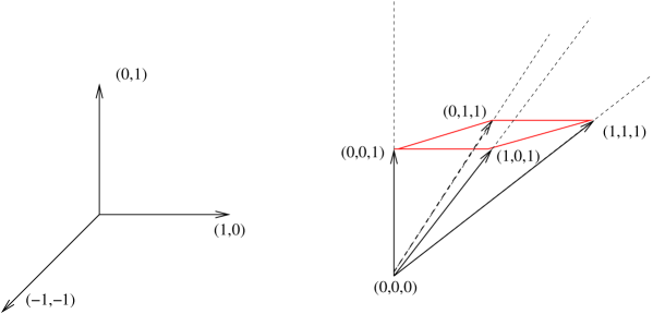
Figure 1: On the left: the fan for $\mathbb{P}^{2}$ with three maximal cones of dimension two which fill completely $\mathbb{R}^{2}$; there are three one dimensional cones in $\Sigma(1)$ with generators $\{(1,0),(0,1),(-1,-1)\}$. On the right: the fan for the conifold with a single maximal cone of dimension three; there are four one dimensional cones in $\Sigma(1)$ with generators $\{(0,0,1),(1,0,1),(1,1,1),(0,1,1)\}$.

We define the variety $V_{\Sigma}$ as a symplectic quotient [44, 43]. Consider the one dimensional cones of $\Sigma$ and a minimal integer generator $n_{i}$ of each of them. Call the set of one dimensional cones $\Sigma(1)$. Assign a “homogeneous coordinate” $x_{i}$ to each $n_{i}\in\Sigma(1)$. If $d=$ dim$\Sigma(1)$, $x_{i}$ span $\mathbb{C}^{d}$. Consider the group

$$G=\{(\mu_{1},...,\mu_{d}\}\in(\mathbb{C}^{*})^{d}|\prod_{i=1}^{d}\mu_{i}^{<m,n_{i}>}=1\,,\,\,\,\,m\in\mathbb{Z}^{3}\}\,,$$ (2.1)

which acts on $x_{i}$ as

$$(x_{1},...,x_{d})\rightarrow(\mu_{1}x_{1},...,\mu_{d}x_{d})\,.$$

$G$ is isomorphic, in general, to $(\mathbb{C}^{*})^{d-n}$ times a discrete group. The continuous part $(\mathbb{C}^{*})^{d-n}$ can be described as follows. Since $d\geqslant n$ the $n_{i}$ are not linearly independent. They determine $d-n$ linear relations:

$$\sum_{i=1}^{d}Q^{(a)}_{i}n_{i}=0$$ (2.2)

with $a=1,...,d-n$ and $Q_{i}^{(a)}$ generate a $(\mathbb{C}^{*})^{d-n}$ action on $\mathbb{C}^{d}$:

$$(x_{1},...,x_{d})\rightarrow(\mu^{Q_{1}^{(a)}}x_{1},...,\mu^{Q_{d}^{(a)}}x_{d})$$ (2.3)

where $\mu\in\mathbb{C}^{*}$.

For each maximal cone $\sigma\in\Sigma$ define the function $f_{\sigma}=\prod_{n_{i}\notin\sigma}x_{i}$ and the locus $S$ as the intersection of all the hypersurfaces $f_{\sigma}=0$. Then the toric variety is defined as:

$$V_{\Sigma}=(\mathbb{C}^{d}-S)/G$$

There is a residual $(\mathbb{C}^{*})^{n}$ complex torus action acting on $V_{\Sigma}$, from which the name toric variety. In the following, we will denote with $T^{n}\equiv U(1)^{n}$ the real torus contained in $(\mathbb{C}^{*})^{n}$.

In all the examples in this paper $G=(\mathbb{C}^{*})^{d-n}$ and the previous quotient is interpreted as a symplectic reduction. The case where $G$ contains a discrete part includes further orbifold quotients. These cases can be handled similarly to the ones discussed in the main text.

Using these rules to construct the toric variety, it is easy to recover the usual representation for $\mathbb{P}^{n}$:

$$\mathbb{P}^{n}=(\mathbb{C}^{n+1}-\{0\})/\{x\sim\mu x\}$$

where the the minimal integer generators of $\Sigma(1)$ are $n_{i}=\{e_{1},...,e_{n},-\sum_{k=1}^{n}e_{k}\}$, $d=n+1$ and $Q=(1,...,1)$ (see Figure 1 for the case $n=2$).

In this paper we will be interested in affine toric varieties, where the fan is a single cone $\Sigma$ = $\sigma$. In this case $S$ is always the null set. It is easy, for example, to find the symplectic quotient representation of the conifold:

$$C(T^{1,1})=\mathbb{C}^{4}/(1,-1,1,-1)$$

where $d=4$, $n=3$, $n_{1}=(0,0,1)$, $n_{2}=(1,0,1)$, $n_{3}=(1,1,1)$, $n_{4}=(0,1,1)$ and we have written $(1,-1,1,-1)$ for the action of $\mathbb{C}^{*}$ with charges $Q=(1,-1,1,-1)$.

This type of description of a toric variety is the easiest one to study divisors and line bundles. Each $n_{i}\in\Sigma(1)$ determines a $T$-invariant divisor $D_{i}$ corresponding to the zero locus $\{x_{i}=0\}$ in $V_{\Sigma}$. $T$-invariant means that $D_{i}$ is mapped to itself by the torus action $(\mathbb{C}^{*})^{n}$ (for simplicity we will call them simply divisors from now on). The $d$ divisors $D_{i}$ are not independent but satisfy the $n$ basic equivalence relations:

$$\sum_{i=1}^{d}<e_{k},n_{i}>D_{i}=0$$ (2.4)

where $e_{k}$ with $k=1,...,n$ is the orthonormal basis of the dual lattice $M\sim\mathbb{Z}^{n}$ with the natural paring: for $n\in N$, $m\in M$ $<n,m>=\sum_{i=1}^{n}n_{i}m_{i}$ $\in\mathbb{Z}$. Given the basic divisors $D_{i}$ the generic divisor $D$ is given by the formal sum $D=\sum_{i=1}^{d}c_{i}D_{i}$ with $c_{i}\in\mathbb{Z}$. Every divisor $D$ determines a line bundle $\mathcal{O}(D)$ .

There exists a simple recipe to find the holomorphic sections of the line bundle $\mathcal{O}(D)$. Given the $c_{i}$, the global sections of $\mathcal{O}(D)$ can be determined by looking at the polytope (a convex rational polyhedron in $M_{\mathbb{R}}$):

$$P_{D}=\{u\in M_{\mathbb{R}}|<u,n_{i}>\hbox{ }\geq\hbox{ }-c_{i}\hbox{ },\hbox{ }\forall i\in\Sigma(1)\}$$ (2.5)

where $M_{\mathbb{R}}=M\otimes_{\mathbb{Z}}\mathbb{R}$. Using the homogeneous coordinate $x_{i}$ it is easy to associate a section $\chi^{m}$ to every point $m$ in $P_{D}$:

$$\chi^{m}=\prod_{i=1}^{d}x_{i}^{<m,n_{i}>+c_{i}}.$$ (2.6)

Notice that the exponent is equal or bigger than zero. Hence the global sections of the line bundle $\mathcal{O}(D)$ over $V_{\Sigma}$ are:

$$H^{0}(V_{\Sigma},\mathcal{O}_{V_{\Sigma}}(D))=\bigoplus_{m\in P_{D}\cap M}\mathbb{C}\cdot\chi^{m}$$ (2.7)

At this point it is important to make the following observation: all monomials $\chi^{m}$ have the same charges under the $(\mathbb{C}^{*})^{d-n}$ described at the beginning of this Section (in the following these charges will be identified with the baryonic charges of the dual gauge theory). Indeed, under the $(\mathbb{C}^{*})^{d-n}$ action we have:

$$\chi^{m}\rightarrow\prod_{i=1}^{d}(\mu^{<m,Q_{i}^{(a)}n_{i}>+Q_{i}^{(a)}c_{i}})x_{i}^{<m,n_{i}>+c_{i}}=\mu^{\sum_{i=1}^{d}Q_{i}^{(a)}c_{i}}\chi^{m}$$ (2.8)

where we have used equation (2.2). Similarly, all the sections have the same charge under the discrete part of the group $G$. This fact has an important consequence. The generic polynomial

$$f=\sum a_{m}\chi^{m}\in H^{0}(V_{\Sigma},\mathcal{O}_{V_{\Sigma}}(D))$$

is not a function on $V_{\Sigma}$, since it is not invariant under the $(\mathbb{C}^{*})^{d-n}$ action (and under possible discrete orbifold actions). However, it makes perfectly sense to consider the zero locus of $f$. Since all monomials in $f$ have the same charge under $(\mathbb{C}^{*})^{d-n}$, the equation $f=0$ is well defined on $V_{\Sigma}$ and defines a divisor .

2.1 A simple Example

After this general discussion, let us discuss an example to clarify the previous definitions.

Consider the toric variety $\mathbb{P}^{2}$. The fan $\Sigma$ for $\mathbb{P}^{2}$ is generated by:

$$n_{1}=e_{1}\hbox{ }n_{2}=e_{2}\hbox{ }n_{3}=-e_{1}-e_{2}$$ (2.9)

The three basic divisors $D_{i}$ correspond to $\{x_{1}=0\}$, $\{x_{2}=0\}$, $\{x_{3}=0\}$, and they satisfy the following relations (see equation (2.4)):

$$D_{1}-D_{3}=0$$

$$D_{2}-D_{3}=0$$

and hence $D_{1}\sim D_{2}\sim D_{3}\sim D$. All line bundles on $\mathbb{P}^{2}$ are then of the form ${\cal O}(nD)$ with an integer $n$, and are usually denoted as ${\cal O}(n)\rightarrow\mathbb{P}^{2}$. It is well known that the space of global holomorphic sections of ${\cal O}(n)\rightarrow\mathbb{P}^{2}$ is given by the homogeneous polynomial of degree $n$ for $n\geq 0$, while it is empty for negative $n$. We can verify this statement using the general construction with polytopes.

Consider the line bundle $\mathcal{O}(D_{1})$ associated with the divisor $D_{1}$. In order to construct its global sections we must first determine the polytope $P_{D_{1}}$ ($c_{1}=1,c_{2}=c_{3}=0$):

$$P_{D_{1}}=\{u_{1}\geqslant-1,\hbox{ }u_{2}\geqslant 0,\hbox{ }u_{1}+u_{2}\leqslant 0\}$$ (2.10)

Then, using (2.6), it easy to find the corresponding sections:

$$\{x_{1},\hbox{ }x_{2},\hbox{ }x_{3}\}$$ (2.11)

These are the homogeneous monomials of order one over $\mathbb{P}^{2}$. Indeed we have just constructed the line bundle $\mathcal{O}(1)\rightarrow\mathbb{P}^{2}$ (see Figure 2).

Consider as a second example the line bundle $\mathcal{O}(D_{1}+D_{2}+D_{3})$. In this case the associated polytope is:

$$P_{D_{1}+D_{2}+D_{3}}=\{u_{1}\geqslant-1,\hbox{ }u_{2}\geqslant-1,\hbox{ }u_{1}+u_{2}\leqslant 1\}$$ (2.12)

Using (2.6) it is easy to find the corresponding sections:

$$\{x_{1}^{3},\hbox{ }x_{1}^{2}x_{2},\hbox{ }x_{1}x_{2}x_{3},...\}$$ (2.13)

These are all the homogeneous monomials of degree $3$ over $\mathbb{P}^{2}$; we have indeed constructed the line bundle $\mathcal{O}(3)\rightarrow\mathbb{P}^{2}$ (see Figure 2).

The examples of polytopes and line bundles presented in this Section are analogous to the ones that we will use in the following to characterize the $BPS$ baryonic operators. The only difference (due to the fact that we are going to consider affine toric varieties) is that the polytope $P_{D}$ will be a non-compact rational convex polyhedron, and the space of sections will be infinite dimensional.

Figure 2: (a) The polytope associated to the line bundle $\mathcal{O}(1)\rightarrow\mathbb{P}^{2}$. (b) The polytope associated to the line bundle $\mathcal{O}(3)\rightarrow\mathbb{P}^{2}$.

3 BPS D3 brane configurations

In this Section we discuss Beasley’s prescription [39] for determining the BPS Hilbert space corresponding to supersymmetric D3 brane configurations. We generalize the example of the conifold presented in [39] to the case of a generic toric Calabi-Yau cone.

3.1 Motivations

Consider the supersymmetric background of type $IIB$ supergravity $AdS_{5}\times H$ with $H$ a Sasaki-Einstein manifold. This geometry is obtained by taking the near horizon geometry of a stack of $N$ $D3$ on the isolated Goreinstein singularity of a local Calabi-Yau three-fold given by the real cone $C(H)$ over the base $H$. The D3 branes fill the four dimensional Minkowski space-time $M_{4}$ in $M_{4}\times C(H)$.

The dual superconformal field theory is a quiver gauge theory: an $\mathcal{N}=1$ supersymmetric quantum field theory with gauge group $SU(N_{1})\times...SU(N_{k})$ and chiral superfields that transform under the fundamental of a gauge group and the anti-fundamental of another gauge group. Due to the presence of $SU(N)$ type groups these theories have generically baryonic like operators inside their spectrum and these are the objects we are interested in.

Let us take the field theory dual to the conifold singularity as a basic example. The theory has gauge group $SU(N)\times SU(N)$ and chiral superfields $A_{1}$, $A_{2}$ that transform under the fundamental of the first gauge group and under the anti-fundamental of the second one, and $B_{1}$, $B_{2}$ that transform under the conjugate representation. There exists also a non-abelian global symmetry $SU(2)\times SU(2)$ under which the $A$ fields transform as $(2,1)$ and the $B$ as $(1,2)$. The superpotential is $W=\epsilon_{ij}\epsilon_{pq}A_{i}B_{p}A_{j}B_{q}$. It is known that this theory has one baryonic charge and that the $A_{i}$ fields have charge one under this symmetry and the $B_{i}$ fields have charge minus one. Hence one can build the two basic baryonic operators:

$$\epsilon^{1}_{p_{1},...,p_{N}}\epsilon_{2}^{k_{1},...,k_{N}}(A_{i_{1}})^{p_{1}}_{k_{1}}...(A_{i_{N}})^{p_{N}}_{k_{N}}=(\det A)_{(i_{1},...,i_{N})}$$

$$\epsilon^{1}_{p_{1},...,p_{N}}\epsilon_{2}^{k_{1},...,k_{N}}(B_{i_{1}})^{p_{1}}_{k_{1}}...(B_{i_{N}})^{p_{N}}_{k_{N}}=(\det B)_{(i_{1},...,i_{N})}$$ (3.1)

These operators are clearly symmetric in the exchange of the $A_{i}$ and $B_{i}$ respectively, and transform under $(N+1,1)$ and $(1,N+1)$ representation of $SU(2)\times SU(2)$. The important observation is that these are the baryonic operators with the smallest possible dimension: $\Delta_{\det A,\det B}=N\Delta_{A,B}$. One can clearly construct operator charged under the baryonic symmetry with bigger dimension in the following way. Defining the operators [46, 39]

$$A_{I;J}=A_{i_{1}}B_{j_{1}}...A_{i_{m}}B_{j_{m}}A_{i_{m+1}}$$ (3.2)

the generic type $A$ baryonic operator is:

$$\epsilon^{1}_{p_{1},...,p_{N}}\epsilon_{2}^{k_{1},...,k_{N}}(A_{I_{1};J_{1}})^{p_{1}}_{k_{1}}...(A_{I_{N};J_{N}})^{p_{N}}_{k_{N}}\,.$$ (3.3)

One can clearly do the same with the type $B$ operators.

Using the tensor relation

$$\epsilon_{\alpha_{1}...\alpha_{N}}\epsilon^{\beta_{1}...\beta_{N}}=\delta^{\beta_{1}}_{[\alpha_{1}}...\delta^{\beta_{N}}_{\alpha_{N}]}\,,$$ (3.4)

depending on the symmetry of (3.3), one can sometimes factorize the operator in a basic baryon times operators that are neutral under the baryonic charge [46, 39]. It is a notorious fact that the $AdS/CFT$ correspondence maps the basic baryonic operators (3.1) to static $D3$ branes wrapping specific three cycles of $T^{1,1}$ and minimizing their volumes. The volumes of the $D3$ branes are proportional to the dimension of the dual operators in $CFT$. Intuitively, the geometric dual of an operator (3.3) is a fat brane wrapping a three cycle, not necessarily of minimal volume, and moving in the $T^{1,1}$ geometry (we will give more rigorous arguments below). If we accept this picture the factorizable operators in field theory can be interpreted in the geometric side as the product of gravitons/giant gravitons states with a static $D3$ brane wrapped on some cycle, and the non-factorisable ones are interpreted as excitation states of the basic $D3$ branes or non-trivial brane configurations.

What we would like to do is to generalize this picture to a generic conical $CY$ singularity. Using a clever parametrization of the possible $D3$ brane $BPS$ configurations in the geometry found in [38, 39], we will explain how it is possible to characterize all the baryonic operators in the dual $SCFT$, count them according to their charges and extract geometric information regarding the cycles.

3.2 Supersymmetric D3 brane configurations

Consider supersymmetric $D3$ branes wrapping three-cycles in $H$. There exists a general characterization of these types of configurations [38, 39] that relates the $D3$-branes wrapped on $H$ to holomorphic four cycles in $C(H)$. The argument goes as follows. Consider the euclidean theory on $\mathbb{R}^{4}\times C(H)$. It is well known that one $D3$-brane wrapping a holomorphic surface $S$ in $C(H)$ preserves supersymmetry. If we put $N$ $D3$-branes on the tip of the cone $C(H)$ and take the near horizon limit the supergravity background becomes $Y_{5}\times H$ where $Y_{5}$ is the euclidean version of $AdS_{5}$. We assume that $S$ intersects $H$ in some three-dimensional cycle $C_{3}$. The $BPS$ $D3$ brane wrapped on $S$ looks like a point in $\mathbb{R}^{4}$ and like a line in $Y_{5}$: it becomes a brane wrapped on a four-dimensional manifold in $\gamma\times H$ where $\gamma$ is the geodesic in $Y_{5}$ obtained from the radial direction in $C(H)$. Using the $SO(5,1)$ global symmetry of $Y_{5}$ we can rotate $\gamma$ into any other geodesic in $Y_{5}$. For this reason when we make the Wick rotation to return to Minkowski signature (this procedure preserves supersymmetry) we may assume that $\gamma$ becomes a time-like geodesic in $AdS_{5}$ spacetime. In this way we have produced a supersymmetric $D3$ brane wrapped on a three cycle in $H$ which moves along $\gamma$ in $AdS_{5}$. Using the same argument in the opposite direction, we realize also that any supersymmetric $D3$ brane wrapped on $H$ can be lifted to a holomorphic surface $S$ in $C(H)$.

Due to this characterization, we can easily parametrize the classical phase space $\mathcal{M}_{cl}$ of supersymmetric $D3$ brane using the space of holomorphic surfaces in $C(H)$ without knowing the explicit metric on the Sasaki-Einstein space $H$ (which is generically unknown!).

The previous construction characterizes all kind of supersymmetric configurations of wrapped D3 branes. These include branes wrapping trivial cycles and stabilized by the combined action of the rotation and the RR flux, which are called giant gravitons in the literature [36]. Except for a brief comment on the relation between giant gravitons and dual giant gravitons, we will be mostly interested in D3 branes wrapping non trivial cycles. These correspond to states with non zero baryonic charges in the dual field theory. The corresponding surface $D$ in $C(H)$ is then a non trivial divisor, which, modulo subtleties in the definition of the sheaf ${\cal O}(D)$, can be written as the zero locus of a section of ${\cal O}(D)$

$$\chi=0\,\qquad\qquad\qquad\chi\in H^{0}(X,{\cal O}(D))$$ (3.5)

3.2.1 The toric case

The previous discussion was general for arbitrary Calabi-Yau cones $C(H)$. From now on we will mostly restrict to the case of an affine toric Calabi-Yau cone $C(H)$. For this type of toric manifolds the fan $\Sigma$ described in Section 2 is just a single cone $\sigma$, due to the fact that we are considering a singular affine variety. Moreover, the Calabi-Yau nature of the singularity requires that all the generators of the one dimensional cone in $\Sigma(1)$ lie on a plane; this is the case, for example, of the conifold pictured in Figure 1. We can then characterize the variety with the convex hull of a fixed number of integer points in the plane: the toric diagram (Figure 3). For toric varieties, the equation for the D3 brane configuration can be written quite explicitly using homogeneous coordinates. As explained in Section 2, we can associate to every vertex of the toric diagram a global homogeneous coordinate $x_{i}$. Consider a divisor $D=\sum c_{i}D_{i}$. All the supersymmetric configurations of D3 branes corresponding to surfaces linearly equivalent to $D$ can be written as the zero locus of the generic section of $H^{0}(V_{\Sigma},\mathcal{O}_{V_{\Sigma}}(D))$

$$P(x_{1},x_{2},...,x_{d})\equiv\sum_{m\in P_{D}\cap M}h_{m}\chi^{m}=0$$ (3.6)

As discussed in Section 2, the sections take the form of the monomials (2.6)

$$\chi^{m}=\prod_{i=1}^{d}x_{i}^{<m,n_{i}>+c_{i}}$$

and there is one such monomial for each integer point $m\in M$ in the polytope $P_{D}$ associated with $D$ as in equation (2.5)

$$\{u\in M_{\mathbb{R}}|<u,n_{i}>\hbox{ }\geq\hbox{ }-c_{i}\hbox{ },\hbox{ }\forall i\in\Sigma(1)\}$$

As already noticed, the $x_{i}$ are only defined up to the rescaling (2.3) but the equation $P(x_{1},...x_{d})=0$ makes sense since all monomials have the same charge under $(\mathbb{C}^{*})^{d-3}$ (and under possible discrete orbifold actions). Equation (3.6) generalizes the familiar description of hypersurfaces in projective spaces $\mathbb{P}^{n}$ as zero locus of homogeneous polynomials. In our case, since we are considering affine varieties, the polytope $P_{D}$ is non-compact and the space of holomorphic global sections is infinite dimensional.

We are interested in characterizing the generic supersymmetric $D3$ brane configuration with a fixed baryonic charge. We must therefore understand the relation between divisors and baryonic charges: it turns out that there is a one-to one correspondence between baryonic charges and classes of divisors modulo the equivalence relation (2.4) . We will understand this point by analyzing in more detail the $(\mathbb{C}^{*})^{d-3}$ action defined in Section 2.

3.2.2 The assignment of charges

To understand the relation between divisors and baryonic charges, we must make a digression and recall how one can assign $U(1)$ global charges to the homogeneous coordinates associated to a given toric diagram [10, 12, 19, 20].

Non-anomalous $U(1)$ symmetries play a very important role in the dual gauge theory and it turns out that we can easily parametrize these global symmetries directly from the toric diagram. In a sense, we can associate field theory charges directly to the homogeneous coordinates.

For a background with horizon $H$, we expect $d-1$ global non-anomalous symmetries, where $d$ is number of vertices of the toric diagram . We can count these symmetries by looking at the number of massless vectors in the $AdS$ dual. Since the manifold is toric, the metric has three isometries $U(1)^{3}\equiv T^{3}$, which are the real part of the $(\mathbb{C}^{*})^{3}$ algebraic torus action. One of these, generated by the Reeb vector, corresponds to the R-symmetry while the other two give two global flavor symmetries in the gauge theory. Other gauge fields in $AdS$ come from the reduction of the RR four form on the non-trivial three-cycles in the horizon manifold $H$, and there are $d-3$ three-cycles in homology [12]. On the field theory side, these gauge fields correspond to baryonic symmetries. Summarizing, the global non-anomalous symmetries are:

$$U(1)^{d-1}=U(1)^{2}_{F}\times U(1)^{d-3}_{B}$$ (3.7)

In this paper we use the fact that these $d-1$ global non-anomalous charges can be parametrized by $d$ parameters $a_{1},a_{2},\ldots,a_{d}$, each associated with a vertex of the toric diagram (or a point along an edge), satisfying the constraint:

$$\sum_{i=1}^{d}a_{i}=0$$ (3.8)

The $d-3$ baryonic charges are those satisfying the further constraint [12]:

$$\sum_{i=1}^{d}a_{i}n_{i}=0$$ (3.9)

where $n_{i}$ are the vectors of the fan: $n_{i}=(y_{i},z_{i},1)$ with $(y_{i},z_{i})$ the coordinates of integer points along the perimeter of the toric diagram. The R-symmetries are parametrized with the $a_{i}$ in a similar way of the other non-baryonic global symmetry, but they satisfy the different constraint

$$\sum_{i=1}^{d}a_{i}=2$$ (3.10)

due to the fact that the terms in the superpotential must have $R$-charges equal to two.

Figure 3: A generic toric diagram with the associated trial charges $a_{i}$, homogeneous coordinates $x_{i}$ and divisors $D_{i}$.

Now that we have assigned trial charges to the vertices of a toric diagram and hence to the homogeneous coordinates $x_{i}$, we can return to the main problem of identifying supersymmetric D3 branes with fixed baryonic charge. Comparing equation (2.2) with equation (3.9), we realize that the baryonic charges $a_{i}$ in the dual field theory are the charges $Q^{(a)}_{i}$ of the action of $(\mathbb{C}^{*})^{d-3}$ on the homogeneous coordinates $x_{i}$. We can now assign a baryonic charge to each monomials made with the homogeneous coordinates $x_{i}$. All terms in the equation (3.6) corresponding to a D3 brane wrapped on $D$ are global sections $\chi^{m}$ of the line bundle $\mathcal{O}(\sum_{i=1}^{d}c_{i}D_{i})$ and they have all the same $d-3$ baryonic charges $B^{a}=\sum_{i=1}^{d}Q_{i}^{(a)}c_{i}$; these are determined only in terms of the $c_{i}$ defining the corresponding line bundle (see equation (2.8)).

Using this fact we can associate a divisor in $C(H)$ to every set of $d-3$ baryonic charges. The procedure is as follows. Once we have chosen a specific set of baryonic charges $B^{a}$ we determine the corresponding $c_{i}$ using the relation $B^{a}=\sum_{i=1}^{d}c_{i}Q_{i}^{(a)}$. These coefficients define a divisor $D=\sum_{i=1}^{d}c_{i}D_{i}$. It is important to observe that, due to equation (2.2), the $c_{i}$ are defined only modulo the equivalence relation $c_{i}\sim c_{i}+<m,n_{i}>$ corresponding to the fact that the line bundle $\mathcal{O}(\sum_{i=1}^{d}c_{i}D_{i})$ is identified only modulo the equivalence relations (2.4) $D\sim D+\sum_{i=1}^{d}<m,n_{i}>D_{i}$. We conclude that baryonic charges are in one-to-one relation with divisors modulo linear equivalence.

For simplicity, we only considered continuous baryonic charges. In the case of varieties which are orbifolds, the group $G$ in equation (2.1) contains a discrete part. In the orbifold case, the quantum field theory contains baryonic operators with discrete charges. This case can be easily incorporated in our formalism.

3.2.3 The quantization procedure

Now we want to quantize the classical phase space $\mathcal{M}_{cl}$ using geometric quantization [47] following [39].

Considering that $P$ and $\lambda P$ with $\lambda\in\mathbb{C}^{*}$ vanish on the same locus in $C(H)$, it easy to understand that the various distinct surfaces in $C(H)$ correspond to a specific set of $h_{m}$ with $m\in P_{D}\cap M$ modulo the equivalence relation $h_{m}\sim\lambda h_{m}$: this is a point in the infinite dimensional space $\mathbb{CP}^{\infty}$ in which the $h_{m}$ are the homogeneous coordinates. Thus we identify the classical configurations space $\mathcal{M}_{cl}$ of supersymmetric $D3$ brane associated to a specific line bundle $\mathcal{O}(D)$ as $\mathbb{CP}^{\infty}$ with homogeneous coordinates $h_{m}$. A heuristic way to understand the geometric quantization is the following. We can think of the $D3$ brane as a particle moving in $\mathcal{M}_{cl}$ and we can associate to it a wave function $\Psi$ taking values in some holomorphic line bundle $\mathcal{L}$ over $\mathbb{CP}^{\infty}$. The reader should not confuse the line bundle ${\cal L}$, over the classical phase space $\mathcal{M}_{cl}$ of wrapped D3 branes, with the lines bundles ${\cal O}(D)$, which are defined on $C(H)$. Since all the line bundles ${\cal L}$ over a projective space are determined by their degree (i.e. they are of the form $\mathcal{O}(\alpha)$) we have only to find the value of $\alpha$. This corresponds to the phase picked up by the wavefunction $\Psi$ when the $D3$ brane goes around a closed path in $\mathcal{M}_{cl}$. Moving in the phase space $\mathcal{M}_{cl}$ corresponds to moving the $D3$ brane in $H$. Remembering that a $D3$ brane couples to the four form field $C_{4}$ of the supergravity and that the backgrounds we are considering are such that $\int_{H}F_{5}=N$, it was argued in [39] that the wavefunction $\Psi$ picks up the phase $e^{2\pi iN}$ and $\alpha=N$. For this reason $\mathcal{L}=\mathcal{O}(N)$ and the global holomorphic sections of this line bundle over $\mathbb{CP}^{\infty}$ are the degree $N$ polynomials in the homogeneous coordinates $h_{m}$.

Since the $BPS$ wavefunctions are the global holomorphic sections of $\mathcal{L}$, we have that the $BPS$ Hilbert space $\mathcal{H}_{D}$ is spanned by the states:

$$|h_{m_{1}},h_{m_{2}},...,h_{m_{N}}>$$ (3.11)

This is Beasley’s prescription.

We will make a correspondence in the following between $h_{m}$ and certain operators in the field theory with one (or more) couple of free gauge indices

$$h_{m}\,,\qquad\qquad\qquad(O_{m})_{\alpha\beta}\,\,(\rm{or}\,(O_{m})_{\alpha_{1}\beta_{1}...\alpha_{k}\beta_{k}})$$ (3.12)

where the $O_{m}$ are operators with fixed baryonic charge. The generic state in this sector $|h_{m_{1}},h_{m_{2}},...,h_{m_{N}}>$ will be identify with a gauge invariant operator obtained by contracting the $O_{m}$ with one (or more) epsilon symbols. The explicit example of the conifold is discussed in details in [39]: the homogeneous coordinates with charges $(1,-1,1,-1)$ can be put in one-to-one correspondence with the elementary fields $(A_{1},B_{1},A_{2},B_{2})$ which have indeed baryonic charge $(1,-1,1,-1)$. The use of the divisor $D_{1}$ (modulo linear equivalence) allows to study the BPS states with baryonic charge $+1$. It is easy to recognize that the operators $A_{I,J}$ in equation (3.2) have baryonic charge $+1$ and are in one-to-one correspondence with the sections of ${\cal O}(D_{1})$

$$\sum_{m\in P_{D_{1}}\cap M}h_{m}\chi^{m}=h_{1}x_{1}+h_{3}x_{3}+...$$

The BPS states $|h_{m_{1}},h_{m_{2}},...,h_{m_{N}}>$ are then realized as all the possible determinants, as in equation (3.3).

3.3 Comments on the relation between giant gravitons and dual giant gravitons

Among the $\mathcal{O}(D)$ line bundles there is a special one: the bundle of holomorphic functions $\mathcal{O}$ . It corresponds to the supersymmetric $D3$ brane configurations wrapped on homologically trivial three cycles $C_{3}$ in $H$ (also called giant gravitons [36]).

When discussing trivial cycles, we can parameterize holomorphic surfaces just by using the embedding coordinates . Our discussion here can be completely general and not restricted to the toric case. Consider the general Calabi-Yau algebraic affine varieties $V$ that are cone over some compact base $H$ (they admit at least a $\mathbb{C}^{*}$ action $V=C(H)$). These varieties are the zero locus of a collection of polynomials in some $\mathbb{C}^{k}$ space. We will call the coordinates of the $\mathbb{C}^{k}$ the embedding coordinates $z_{j}$, with $j=1,...,k$. The coordinate rings $\mathbb{C}[V]$ of the varieties $V$ are the restriction of the polynomials in $\mathbb{C}^{k}$ of arbitrary degree on the variety $V$:

$$\mathbb{C}[V]=\frac{\mathbb{C}[z_{1},...z_{k}]}{\{p_{1},...,p_{l}\}}=\frac{\mathbb{C}[z_{1},...z_{k}]}{\mathbb{I}[V]}$$ (3.13)

where $\mathbb{C}[z_{1},...,z_{k}]$ is the $\mathbb{C}$-algebra of polynomials in $k$ variables and $p_{j}$ are the defining equations of the variety $V$. We are going to consider the completion of the coordinate ring (potentially infinity polynomials) whose generic element can be written as the (infinite) polynomial in $\mathbb{C}^{k}$

$$P(z_{1},...z_{k})=c+c_{i}z_{i}+c_{ij}z_{i}z_{j}+...=\sum_{I}c_{I}z_{I}$$ (3.14)

restricted by the algebraic relations $\{p_{1}=0,...,p_{l}=0\}$.

At this point Beasley’s prescription says that the $BPS$ Hilbert space of the giant gravitons $\mathcal{H}_{g}$ is spanned by the states

$$|c_{I_{1}},c_{I_{2}},...,c_{I_{N}}>$$ (3.15)

These states are holomorphic polynomials of degree $N$ over $\mathcal{M}_{cl}$ and are obviously symmetric in the $c_{I_{i}}$. For this reason we may represent (3.15) as the symmetric product:

$$Sym(|c_{I_{1}}>\otimes|c_{I_{2}}>\otimes...\otimes|c_{I_{N}}>)$$ (3.16)

Every element $|c_{I_{i}}>$ of the symmetric product is a state that represents a holomorphic function over the variety $C(H)$. This is easy to understand if one takes the polynomial $P(z_{1},...z_{k})$ and consider the relations among the $c_{I}$ induced by the radical ring $\mathbb{I}[V]$ (in a sense one has to quotient by the relations generated by $\{p_{1}=0,...,p_{l}=0\}$). For this reason the Hilbert space of giant gravitons is:

$$\mathcal{H}_{g}=\bigotimes^{N\hbox{ }Sym}\mathcal{O}_{C(H)}$$ (3.17)

Obviously, we could have obtained the same result in the toric case by applying the techniques discussed in this Section. Indeed if we put all the $c_{i}$ equal to zero the polytope $P_{D}$ reduces to the dual cone $\mathcal{C}^{*}$ of the toric diagram, whose integer points corresponds to holomorphic functions on $C(H)$ [35].

In a recent work [34] it was shown that the Hilbert space of a dual giant graviton $\mathcal{H}_{dg}$ in the background space $AdS_{5}\times H$, where $H$ is a generic Sasaki-Einstein manifold, is the space of holomorphic functions over the cone $C(H)$.  At this point it is easy to understand why the counting of $1/2$ $BPS$ states of giant gravitons and dual giant gravitons give the same result[32, 31]: the counting of $1/2$ $BPS$ mesonic state in field theory. Indeed:

$$\mathcal{H}_{g}=\bigotimes^{N\hbox{ }Sym}\mathcal{H}_{dg}$$ (3.18)

4 Flavor charges of the BPS baryons

In the previous Section, we discussed supersymmetric $D3$ brane configurations with specific baryonic charge. Now we would like to count, in a sector with given baryonic charge, the states with a given set of flavor charges $U(1)\times U(1)$ and $R$-charge $U(1)_{R}$. The generic state of the $BPS$ Hilbert space (3.11) is, by construction, a symmetric product of the single states $|h_{m}>$. These are in a one to one correspondence with the integer points in the polytope $P_{D}$, which correspond to sections $\chi^{m}$. As familiar in toric geometry [44, 43], a integer point $m\in M$ contains information about the charges of the $T^{3}$ torus action, or, in quantum field theory language, about the flavor and $R$ charges.

Now it is important to realize that, as already explained in Section 3, the charges $a_{i}$ that we can assign to the homogeneous coordinates $x_{i}$ contain information about the baryonic charges (we have already taken care of them) but also about the flavor and $R$ charges in the dual field theory. If we call $f^{k}_{i}$ with $k=1,2$ the two flavor charges and $R_{i}$ the $R$-charge, the section $\chi^{m}$ has flavor charges (compare equation (2.6)):

$$f^{k}_{m}=\sum_{i=1}^{d}(<m,n_{i}>+c_{i})f^{k}_{i}$$ (4.1)

and $R$-charge:

$$R_{m}=\sum_{i=1}^{d}(<m,n_{i}>+c_{i})R_{i}$$ (4.2)

It is possible to refine the last formula. Indeed the $R_{i}$, which are the R-charges of a set of elementary fields of the gauge theory [12, 19] , are completely determined by the Reeb vector of $H$ and the vectors $n_{i}$ defining the toric diagram [17]. Moreover, it is possible to show that $\sum_{i=1}^{d}n_{i}R_{i}=\frac{2}{3}b$ [19], where $b$ specifies how the Reeb vector lies inside the $T^{3}$ toric fibration. Hence:

$$R_{m}=\frac{2}{3}<m,b>+\sum_{i=1}^{d}c_{i}R_{i}$$ (4.3)

This formula generalizes an analogous one for mesonic operators [28]. Indeed if we put all the $c_{i}$ equal to zero the polytope $P_{D}$ reduces to the dual cone $\mathcal{C}^{*}$ of the toric diagram [35]. We know that the elements of the mesonic chiral ring of the $CFT$ correspond to integer points in this cone and they have $R$-charge equal to $\frac{2}{3}<m,b>$. In the case of generic $c_{i}$, the right most factor of (4.3) is in a sense the background $R$ charge: the $R$ charge associated to the fields carrying the non-trivial baryonic charges. In the simple example of the conifold discussed in subsection 3.1, formula (4.3) applies to the operators (3.2) where the presence of an extra factor of $A$ takes into account the background charge. In general the R charge (4.3) is really what we expect from an operator in field theory that is given by elementary fields with some baryonic charges dressed by “mesonic insertions”.

The generic baryonic configuration is constructed by specifying $N$ integer points $m_{\rho}$ in the polytope $P_{D}$. Its $R$ charge $R_{B}$ is

$$R_{B}=\frac{2}{3}\sum_{\rho=1}^{N}<m_{\rho},b>+N\sum_{i=1}^{d}c_{i}R_{i}$$ (4.4)

This baryon has $N$ times the baryonic charges of the associated polytope. Recalling that at the superconformal fixed point dimension $\Delta$ and $R$-charge of a chiral superfield are related by $R=2\Delta/3$, it is easy to realize that the equation (4.4) is really what is expected for a baryonic object in the dual superconformal field theory. Indeed if we put all the $m_{\rho}$ equal to zero we have (this means that we are putting to zero all the mesonic insertions)

$$\Delta_{B}=N\sum_{i=1}^{d}c_{i}\Delta_{i}$$ (4.5)

This formula can be interpreted as follows. The elementary divisor $D_{i}$ can be associated with (typically more than one) elementary field in the gauge theory, with R charge $R_{i}$. By taking just one of the $c_{i}$ different from zero in formula (4.5), we obtain the dimension of a baryonic operator in the dual field theory: take a fixed field, compute its determinant and the dimension of the operator is $N$ times the dimension of the individual fields. These field operators correspond to $D3$ branes wrapped on the basic divisors $D_{i}$ and are static branes in the $AdS_{5}\times H$ background . They wrap the three cycles $C_{3}^{i}$ obtained by restricting the elementary divisors $D_{i}$ at $r=1$. One can also write the $R_{i}$ in terms of the volume of the Sasaki-Einstein space $H$ and of the volume of $C_{3}^{i}$ [4]:

$$R_{i}=\frac{\pi\hbox{Vol}(C_{3}^{i})}{3\hbox{Vol}(H)}$$ (4.6)

Configurations with more than one non-zero $c_{i}$ in equation (4.5) correspond to basic baryons made with elementary fields whose R-charge is a linear combination of the $R_{i}$ (see [19]) or just the product of basic baryons.

The generic baryonic configuration has $N$ times the $R$-charge and the global charges of the basic baryons (static branes which minimize the volume in a given homology class) plus the charges given by the fattening and the motion of the three cycle inside the geometry (the mesonic fluctuations on the $D3$ brane or “mesonic insertions” in the basic baryonic operators in field theory). It is important to notice that the BPS operators do not necessarily factorize in a product of basic baryons times mesons .

4.1 Setting the counting problem

In Section 6 we will count the baryonic states of the theory with given baryonic charges (polytope $P_{D}$) according to their $R$ and flavor charges. Right now we understand the space of classical supersymmetric $D3$ brane configurations $\mathcal{N}$ as a direct sum of holomorphic line bundles over the variety $C(H)$:

$$\mathcal{N}=\bigoplus_{c_{i}\sim c_{i}+<m,n_{i}>}\mathcal{O}\Big{(}\sum_{i}^{d}c_{i}D_{i}\Big{)}$$ (4.7)

where the $c_{i}$ specify the baryonic charges. We have just decomposed the space $\mathcal{N}$ into sectors according to the grading given by the baryonic symmetry. Geometrically, this is just the decomposition of the homogeneous coordinate ring of the toric variety under the grading given by the action of $(\mathbb{C}^{*})^{d-3}$. Now, we want to introduce a further grading. Inside every line bundle there are configurations with different flavor and $R$ charges.

Once specified the baryonic charges, the Hilbert space of BPS operators is the $N$ order symmetric product of the corresponding line bundle. Hence the $1/2$ $BPS$ Hilbert space is also decomposed as:

$$\mathcal{H}=\bigoplus_{c_{i}\sim c_{i}+<m,n_{i}>}\mathcal{H}_{D}$$ (4.8)

We would like to count the baryonic operators of the dual $SCFT$ with a given set of flavor and $R$ charges. We can divide this procedure into three steps:

• find a way to count the global sections of a given holomorphic line bundle (a baryonic partition function $Z_{D}$);

• write the total partition function for the $N$-times symmetric product of the polytope $P_{D}$ (the partition function $Z_{D,N}$). This corresponds to find how many combinations there are with the same global charges $a_{B}^{k}$ (with $k=1,2$ for the flavor charges and $k=3$ for the $R$ charge ) for a given baryonic state: the possible set of $m_{\rho}$ such that:

  $$a_{B}^{k}-N\sum_{i=1}^{d}c_{i}a_{i}^{k}=\sum_{m_{\rho}\in P_{D}\cap M}\sum_{i=1}^{d}<m_{\rho},n_{i}>a_{i}^{k}\,.$$ (4.9)

• write the complete $BPS$ partition function of the field theory by summing over all sectors with different baryonic charges. Eventually we would also like to write the complete $BPS$ partition function of the field theory including all the $d$ charges at a time: $d-3$ baryonic, $2$ flavor and $1$ $R$ charges [42].

In the following Sections, we will solve completely the first two steps. The third step is complicated by various facts. First of all the correspondence between the homogeneous coordinates and fields carrying the same $U(1)$ charges is not one to one. From the gravity side of the $AdS/CFT$ correspondence one can explain this fact as follow [12]. The open strings attached to a $D3$ brane wrapped on the non-trivial three cycles corresponding to the basic baryons in the dual field theory have in general many supersymmetric vacuum states. This multiplicity of vacua corresponds to the fact that generically the first homotopy group of the three cycles $\pi_{1}(C_{3})$ is non-trivial and one can turn on a locally flat connection with non-trivial Wilson lines. The different Wilson lines give the different open string vacua and these are associated with different elementary fields $X_{ij}$ (giving rise to basic baryons $\det X_{ij}$ with the same global charges). One has then to include non trivial multiplicities for the $Z_{D,N}$ when computing the complete BPS partition function. Moreover one should pay particular attention to the sectors with higher baryonic charge. All these issues and the determination of the partition function depending on all the $d$ charges will be discussed in forthcoming publications [42].

5 Comparison with the field theory side

At this point it is probably worthwhile to make a more straight contact with the field theory. This is possible at least for all toric CY because the dual quiver gauge theory is known [16, 21, 22]. In this paper we will mainly focus on the partition function $Z_{D}$ for supersymmetric D3 brane configurations. In forthcoming papers [42] we will show how to compute the partition function for the chiral ring and how to compare with the full set of BPS gauge invariant operators. In this Section we show that, for a selected class of polytopes $P_{D}$, there is a simple correspondence between sections of the line bundle $D$ and operators in the gauge theory.

The gauge theory dual to a given toric singularity is completely identified by the dimer configuration, or brane tiling (Figure 4) [16, 21, 22]. This is a bipartite graph drawn on a torus $T^{2}$: it has an equal number of white and black vertices and links connect only vertices of different colors. In the dimer the faces represent $SU(N)$ gauge groups, oriented links represent chiral bifundamental multiplets and nodes represent the superpotential: the trace of the product of chiral fields around a node gives a superpotential term with sign + or - according to whether the vertex is a white one or a black one. By applying Seiberg dualities to a quiver gauge theory we can obtain different quivers that flow in the IR to the same CFT: to a toric diagram we can associate different quivers/dimers describing the same physics. It turns out that one can always find phases where all the gauge groups have the same number of colors; these are called toric phases. Seiberg dualities keep constant the number of gauge groups $F$, but may change the number of fields $E$, and therefore the number of superpotential terms $V=E-F$. The toric phases having the minimal set of fields are called minimal toric phases.

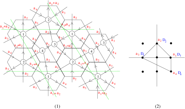
Figure 4: (1) Dimer configuration for the field theory dual to $C(Y^{2,1})$ with a given assignment of charges $a_{i}$ and the orientation given by the arrows connecting the gauge groups. We have drawn in green the bounds of the basic cell. For notational simplicity we have not indicated with different colors the vertices; the dimer is a bipartite graph and this determines an orientation. (2) Toric diagram for the singularity $C(Y^{2,1})$.

There is a general recipe for assigning baryonic, flavors and R charges to the elementary fields for a minimal toric phase of the $CFT$ [10, 12, 19, 20]. As described in Section (3.2.2), we can parameterize all charges with $d$ numbers $a_{i}$, $i=1,...,d$ associated with the vertices of the toric diagram subject to the constraint (3.8) in case of global symmetries and (3.10) in case of R symmetries. Every elementary field can be associated with a brane wrapping a particular divisor

$$D_{i+1}+D_{i+2}+\ldots D_{j}$$ (5.1)

and has charge $a_{i+1}+a_{i+2}+\ldots a_{j}$ . Various fields have the same charge; as mentioned in the last part of the Section 4, this multiplicity is due to the non-trivial homotopy of the corresponding cycles. Explicit methods for computing the charge of each link in the dimer are given in [12, 19]. The specific example of $H=Y^{2,1}$ is reported in Figure 4.

With this machinery in our hands we can analyze the the field theory operators corresponding to the $D3$ brane states analyzed in the previous Sections. The first thing to understand is the map between the section $\chi^{m}$ of the line bundle we are considering and the field theory operators. The case of the trivial line bundle is well known: the corresponding polytope is the cone of holomorphic functions which are in one-to-one correspondence with mesonic operators. The latter are just closed loops in the quiver. It is possible to construct a map between closed loops in the quiver and points in the cone of holomorphic functions; it can be shown that closed loops mapped to the same point in the cone correspond to mesons that are $F$-term equivalent [49, 48].

We would like to do the same with open paths in the dimer. In particular we would like to associate to every point in the polytope $P_{D}$ a sequence of contractions of elementary fields modulo $F$-term equivalence. This is indeed possible for a particular class of polytopes which we now describe.

Let us start by studying open paths in the dimer. Take two gauge group $U$, $V$ in the dimer and draw an oriented path $P$ connecting them (an oriented path in the dimer is a sequence of chiral fields oriented in the same way and with the gauge indices contracted along the path). The global charges of $P$ is the sum of the charges of the fields contained in $P$ and can be schematically written as:

$$\sum_{i=1}^{d}c_{i}a_{i}$$ (5.2)

with some integers $c_{i}$. Draw another oriented path $Q$ connecting the same gauge groups. Consider now the closed non-oriented path $Q-P$; as explained in [48] the charges for a generic non-oriented closed path can be written as :

$$\sum_{i=1}^{d}<m,n_{i}>a_{i}$$ (5.3)

with $m$ a three dimensional integer vector. Hence the charges for a generic path $Q$ connecting two gauge groups are:

$$\sum_{i=1}^{d}(<m,n_{i}>+c_{i})a_{i}\,.$$ (5.4)

Because the path $Q$ is oriented we have just added the charges along it and the coefficients of the $a_{i}$ are all positive:

$$<m,n_{i}>+c_{i}\geqslant 0\,.$$ (5.5)

We have the freedom to change $P$; this means that the $c_{i}$ are only defined up to the equivalence relation $c_{i}\sim c_{i}+<m,n_{i}>$. Observe that (5.5) is the same condition on the exponents for the homogeneous coordinates $x_{i}$ in the global sections $\chi^{m}$ (2.5), and the equivalence relation $c_{i}\sim c_{i}+<m,n_{i}>$ corresponds to the equivalence relation on the divisors $D\sim D+\sum_{i=1}^{d}<m,n_{i}>D_{i}$. Hence we realize that to every path connecting a pair of gauge groups we can assign a point in a polytope associated with the divisor $\sum_{i}c_{i}D_{i}$ modulo linear equivalence. In particular, all operators associated with open paths between two gauge groups $(U,V)$ have the same baryonic charge, as it can be independently checked.

Now that we have a concrete map between the paths in the dimer and the integer points in the polytope we have to show that this map is well defined. Namely we have to show that we map $F$-term equivalent operators to the same point in the polytope and that to a point in the polytope corresponds only one operator in field theory modulo $F$ terms relations (the injectivity of the map). The first step is easy to demonstrate: paths that are $F$-term equivalents have the same set of $U(1)$ charges and are mapped to the same point $m$ in the polytope $P_{D}$. Conversely if paths connecting two gauge groups are mapped to the same point $m$ it means that they have the same global charges. The path $P-P^{\prime}$ is then a closed unoriented path with charge 0. As shown in [49, 48] $P$ and $P^{\prime}$ are then homotopically equivalent . Now we can use the Lemma $5.3.1$ in [49] that says: “in a consistent tiling, paths with the same $R$-charge are $F$-term equivalent if and only if they are homotopic” to conclude that paths mapped to the same point $m$ in $P_{D}$ are $F$-term equivalent. Surjectivity of the map is more difficult to prove, exactly as in the case of closed loops [49, 48], but it is expected to hold in all relevant cases.

In particular we will apply the previous discussion to the case of neighbouring gauge groups $(U,V)$ connected by one elementary field. If the charge of the field is $a_{i+1}+...+a_{j}$ we are dealing with the sections of the line bundle ${\cal O}(D_{i+1}+...+D_{j})$

$$\sum_{m\in P_{D_{i+1}+...+D_{j}}}h_{m}\chi^{m}=h\,x_{i+1}...x_{j}+...$$

The section $x_{i+1}...x_{j}$ will correspond to the elementary field itself while all other sections $\chi^{m_{j}}$ will correspond to operators with two free gauge indices $(O_{m})_{\alpha\beta}$ under $U$ and $V$ which correspond to open paths from $U$ to $V$. The proposal for finding the gauge invariant operator dual to the $BPS$ state $|h_{m_{1}},...,h_{m_{N}}>$ is then the following. We associate to every $h_{m_{j}}$, with section $\chi^{m_{j}}$, an operator in field theory with two free gauge indices in the way we have just described (from now on we will call these paths the building blocks of the baryons). Then we construct a gauge invariant operator by contracting all the $N$ free indices of one gauge group with its epsilon tensor and all the $N$ free indices of the other gauge group with its own epsilon. The field theory operator we have just constructed has clearly the same global charges of the corresponding state in the string theory side and due to the epsilon contractions is symmetric in the permutation of the field theory building blocks like the string theory state. This generalizes Equation (3.3) to the case of a generic field in a toric quiver. By abuse of language, we can say that we have considered all the single determinants that we can make with indices in $(U,V)$.

As already mentioned, D3 branes wrapped on three cycles in $H$ come with a multiplicity which is given by the non trivial homotopy of the three cycle. On the field theory side, this corresponds to the fact there is a multiplicity of elementary fields with the same charge. Therefore a polytope $P_{D}$ is generically associated to various different pairs of gauge groups $(U^{a},V^{a})$, $a=1,...\#_{D}$. For this reason we say that the polytope $P_{D}$ has a multiplicity $\#_{D}$. This implies that there is an isomorphism between the set of open paths (modulo $F$-terms) connecting the different pairs $(U^{a},V^{a})$. Similarly, the single determinant baryonic operators constructed as above from different pairs $(U^{a},V^{a})$ come isomorphically from the point of view of the counting problem.

Obviously, the baryonic operators we have constructed are just a subset of the chiral ring of the toric quiver gauge theory. They correspond to possible single determinants that we can construct. In the case of greater baryonic charge (products of determinants) the relation between points in the polytope $P_{D}$ and operators is less manifest and it will be discussed in section 5.2.

As an example of this construction, we now discuss the baryonic building blocks associated with a line bundle over the Calabi-Yau cone $C(Y^{2,1})$.

5.1 Building blocks for $\mathcal{O}(D_{3})\rightarrow C(Y^{2,1})$

Let us explain the map between the homogeneous coordinates and field theory operators in a simple example: $C(Y^{2,1})$. The cone over $Y^{2,1}$ has four divisors with three equivalence relations (see Figure 4) and hence we have the assignment:

$$D_{1}=3D\qquad D_{2}=-2D\qquad D_{3}=D\qquad D_{4}=-2D$$ (5.6)

We want to construct the building blocks of the $BPS$ operators with baryonic charge equal to one. Because the $(\mathbb{C}^{*})^{d-3}=\mathbb{C}^{*}$ action is specified by the charge:

$$Q=(+3,-2,+1,-2)$$ (5.7)

we choose $c_{3}=1$ and $c_{1}=c_{2}=c_{4}=0$. Hence:

$$P_{D_{3}}=\{m\epsilon M|m_{1}+m_{3}\geq 0,m_{2}+m_{3}\geq 0,-m_{1}+m_{3}\geq-1,m_{1}-m_{2}+m_{3}\geq 0\}$$ (5.8)

We can now easily construct the sections of the corresponding line bundle $\mathcal{O}(D_{3})$ and try to match these with the $BPS$ operators, which are just the open paths in the dimer (see Figure 4) with the same trial charges $a_{i}$ of the polynomial in the homogeneous variables. Looking at the dimer of $Y^{2,1}$ we immediately realize that there are three distinct pairs of gauge groups with charge $\sum_{i=1}^{d}c_{i}a_{i}=a_{3}$: $(2,1)$, $(4,2)$, $(1,3)$. Hence the multiplicity of $P_{D_{3}}$ is $\#_{D_{3}}=3$ and for every point in the polytope we have three different operators in the field theory side, corresponding to paths in the dimer connecting the three different pairs of gauge groups. In Table $1$ we match the sections in the geometry side with the operators in the field theory side for few points in the polytope $P_{D_{3}}$.

$(m_{1},m_{2},m_{3})$	sections	charges	$(2,1)$	$(4,2)$	$(1,3)$
(0,0,0)	$x_{3}$	$a_{3}$	$X_{21}^{dl}=Y$	$X_{42}^{dl}=Y$	$X_{13}^{dl}=Y$
(1,0,0)	$x_{1}x_{4}$	$a_{1}+a_{4}$	$X_{21}^{dr}=V$	$X_{43}^{ur}X_{32}^{dr}=ZU$	$X_{14}^{dr}X_{43}^{ur}=UZ$
(1,1,0)	$x_{1}x_{2}$	$a_{1}+a_{2}$	$X_{21}^{u}=V$	$X_{43}^{ur}X_{32}^{u}=ZU$	$X_{14}^{u}X_{43}^{ur}=UZ$
(-1,0,1)	$x_{2}x_{3}^{3}$	$a_{2}+3a_{3}$	$X_{21}^{dl}X_{14}^{u}X_{42}^{dl}X_{21}^{dl}$	$X_{42}^{dl}X_{21}^{dl}X_{14}^{u}X_{42}^{dl}$	$X_{13}^{dl}X_{32}^{u}X_{21}^{dl}X_{13}^{dl}$
			$=YUYY$	$=YYUY$	$=YUYY$
(-1,-1,1)	$x_{3}^{3}x_{4}$	$3a_{3}+a_{4}$	$X_{21}^{dl}X_{13}^{dl}X_{32}^{dr}X_{21}^{dl}$	$X_{42}^{dl}X_{21}^{dl}X_{14}^{dr}X_{42}^{dl}$	$X_{13}^{dl}X_{32}^{dr}X_{21}^{dl}X_{13}^{dl}$
			$=YYUY$	$=YYUY$	$=YUYY$
…	…	…	…	…	…

Table 1: Few sections of $\mathcal{O}(D_{3})$ and the corresponding field theory operators of baryon number $1$. We write: the point $m$ in the polytope; the corresponding section ($x_{i}$ are the homogeneous coordinates ); its charges; the three corresponding gauge operators ($X$ are the fundamental fields): we used the label $u$, $l$, $d$, $r$ for $up$, $left$, $down$, $right$, to specify the field direction and, for comparison with the literature, the field is also written using the notations commonly adopted for $Y^{p,q}$ [9].

One can observe, by looking at the dimer (Figure 4), that in the fourth and fifth lines of Table $1$ one can assign different operators to the same section, but it is easy to check that these are related by $F$-term equations. Hence in this simple case the correspondence between geometry and field theory is manifest.

The gauge invariant operators with baryonic charge $N$ are obtained by taking all the operators connecting the same gauge groups and by contracting the $N$ free indices of one gauge group with its epsilon and the $N$ free indices of the other gauge group with its own epsilon. All operators come in triples with the same quantum numbers.

5.2 Comments on the general correspondence

In the case of a generic polytope $P_{D}$, not associated with elementary fields, the correspondence between sections of the line bundle ${\cal O}(D)$ and operators is less manifest. The reason is that we are dealing with higher baryonic charges and the corresponding gauge invariant operators are generically products of determinants.

Let us consider as an example the case of the conifold. Suppose we want to study the polytope $P_{2D_{1}}$ which corresponds to classify the $BPS$ operators with baryonic charges equal to $2N$. In field theory we certainly have baryonic operators with charge $2N$, for example $\det A_{1}\cdot\det A_{1}$. Clearly all the products of two baryonic operators with baryon number $N$ give a baryonic operator with baryon number $2N$. In a sense in the conifold all the operators in sectors with baryonic charge with absolute value bigger than one are factorized [46, 39]. However we cannot find a simple prescription for relating sections of $P_{2D_{1}}$ to paths in the dimer. Certainly we can not find a single path in the dimer (Figure 5) connecting the two gauge groups with charge $2a_{1}$.

One could speculate that the prescription valid for basic polytopes has to be generalized by allowing the use of paths and multipaths. For example, to the section $\chi^{m}$ in the polytope $P_{2D_{1}}$ for the conifold we could assign two paths connecting the two gauge groups with charges $\sum_{i=1}^{d}<m^{(1)},n_{i}>+a_{1}$ and $\sum_{i=1}^{d}<m^{(2)},n_{i}>+a_{1}$ with $m=m^{(1)}+m^{(2)}$ and therefore a building block consisting of two operators $(O_{m^{(1)}})_{\alpha_{1}\beta_{1}}(O_{m^{(2)}})_{\alpha_{2}\beta_{2}}$. We should now construct the related gauge invariant operators. Out of these building blocks we cannot construct a single determinant because we don’t have an epsilon symbol with $2N$ indices, but we can easily construct a product operator using four epsilons. We expect, based on Beasley’s prescription, a one to one correspondence between the points in the $N$ times symmetric product of the polytope $P_{2D_{1}}$ and the baryonic operators with baryonic charge $+2$ in field theory. Naively, it would seem that, with the procedure described above, we have found many more operators. Indeed the procedure was plagued by two ambiguities: in the construction of the building blocks, it is possible to find more than a pair of paths corresponding to the same $m$ (and thus the same $U(1)$ charges) that are not $F$-term equivalent; in the construction of the gauge invariants we have the ambiguity on how to distribute the operators between the two determinants. The interesting fact is that these ambiguities seem to disappear when we consider the final results for gauge invariant operators, due to the $F$-term relations and the properties of the epsilon symbol. One can indeed verify, at least in the case of $P_{2D_{1}}$ and for various values of $N$, there is exactly a one to one correspondence between the points in the $N$ times symmetric product of the polytope and the baryonic operators in field theory. It would be interesting to understand if this kind of prescription can be made rigorous.

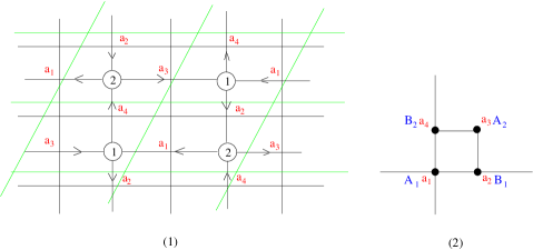
Figure 5: (1) Dimer configuration for the field theory dual to $C(T^{1,1})$ with a given assignment of charges $a_{i}$ and the orientation given by the arrows linking the gauge groups. We have drawn in green the bounds of the basic cell. (2) Toric diagram for the singularity $C(T^{1,1})$.

The ambiguity in making a correspondence between sections of the polytope and operators is expected and it is not particularly problematic. The correct correspondence is between the states $|h_{m_{1}},...,h_{m_{N}}>$ and baryonic gauge invariant operators. The sections in the geometry are not states of the string theory and the paths/operators are not gauge invariant operators. What the $AdS/CFT$ correspondence tells us is that there exists a one to one relation between states in string theory and gauge invariant operators in field theory, and this is a one to one relation between the points in the $N$-fold symmetric product of a given polytope and the full set of gauge invariant operators with given baryonic charge.

The comparison with field theory should be then done as follows. One computes the partition functions $Z_{D,N}$ of the $N$-fold symmetrized product of the polytope $P_{D}$ and compares it with all the gauge invariant operators in the sector of the Hilbert space with given baryonic charge. We have explicitly done it for the conifold for the first few values of $N$ and the operators with lower dimension. In forthcoming papers [42] we will actually resum the partition functions $Z_{D,N}$ and we will write the complete partition function for the chiral ring of the conifold and other selected examples; we will compare the result with the dual field theory finding perfect agreement.

The issues of multiplicities that we already found in the case of polytopes associated with elementary fields persists for generic polytopes. Its complete understanding is of utmost importance for writing a full partition function for the chiral ring [42].

6 Counting BPS baryonic operators

In this Section, as promised, we count the number of BPS baryonic operators in the sector of the Hilbert space $\cal{H}_{D}$, associated with a divisor $D$. All operators in $\cal{H}_{D}$ have fixed baryonic charges. Their number is obviously infinite, but, as we will show, the number of operators with given charge $m\in T^{3}$ under the torus action is finite. It thus makes sense to write a partition function $Z_{D,N}$ for the BPS baryonic operators weighted by a $T^{3}$ charge $q=(q_{1},q_{2},q_{3})$. $Z_{D,N}$ will be a polynomial in the $q_{i}$ such that to every monomial $n\hbox{ }q_{1}^{m_{1}}q_{2}^{m_{2}}q_{3}^{m_{3}}$ we associate $n$ $BPS$ D3 brane states with the R-charge and the two flavor charges parametrized by $\sum_{i=1}^{d}(<m,n_{i}>a_{i}+Nc_{i}a_{i})$.

The computation of the weighted partition function is done in two steps. We first compute a weighted partition function $Z_{D}$, or character, counting the sections of ${\cal O}(D)$; these correspond to the $h_{m}$ which are the elementary constituents of the baryons. In a second time, we determine the total partition function $Z_{D,N}$ for the states $|h_{m_{1}}...h_{m_{N}}>$ in $\cal{H}_{D}$.

6.1 The character $Z_{D}$

We want to resum the character, or weighted partition function,

$$Z_{D}=\rm{Tr}\{q|H^{0}(X,{\cal O}(D)\}=\sum_{m\in P_{D}\cap M}q^{m}$$ (6.1)

counting the integer points in the polytope $P_{D}$ weighted with their charge under the $T^{3}$ torus action.

In the trivial case ${\cal O}(D)\sim{\cal O}$, $Z_{D}$ is just the partition function for holomorphic functions discussed in [35, 33], which can be computed using the Atyah-Singer index theorem [35]. Here we show how to extend this method to the computation of $Z_{D}$ for a generic divisor $D$.

Suppose that we have a smooth variety and a line bundle ${\cal O}(D)$ with a holomorphic action of $T^{k}$ (with $k=1,2,3$ and $k=3$ is the toric case). Suppose also that the higher dimensional cohomology of the line bundle vanishes, $H^{i}(X,{\cal O}(D))=0$, for $i\geq 1$. The character (6.1) then coincides with the Leftschetz number

$$\chi(q,D)=\sum_{p=0}^{3}(-1)^{p}\rm{Tr}\{q|H^{p}(X,{\cal O}(D))\}$$ (6.2)

which can be computed using the index theorem [50]: we can indeed write $\chi(q,D)$ as a sum of integrals of characteristic classes over the fixed locus of the $T^{k}$ action. In this paper, we will only consider cases where $T^{k}$ has isolated fixed points $P_{I}$. The general case can be handled in a similar way. In the case of isolated fixed points, the general cohomological formula considerably simplifies and can be computed by linearizing the $T^{k}$ action near the fixed points. The linearized action can be analysed as follows. Since $P_{I}$ is a fixed point, the group $T^{k}$ acts linearly on the normal (=tangent) space at $P_{I}$, $TX_{P_{I}}\sim\mathbb{C}^{3}$. The tangent space will split into three one dimensional representations $TX_{P_{I}}=\sum_{\lambda=1}^{3}L^{\lambda}$ of the abelian group $T^{k}$. We denote the corresponding weights for the $q$ action with $m_{I}^{\lambda},\lambda=1,2,3$. Denote also with $m_{I}^{0}$ the weight of the action of $q$ on the $\mathbb{C}$ fiber of the line bundle ${\cal O}(D)$ over $P_{I}$. The equivariant Riemann-Roch formula expresses the Leftschetz number as a sum over the fixed points

$$\chi(q,D)=\sum_{P_{I}}\frac{q^{m_{I}^{0}}}{\prod_{\lambda=1}^{3}(1-q^{m_{I}^{\lambda}})}$$ (6.4)

We would like to apply the index theorem to our Calabi-Yau cone. Unfortunately, $X=C(H)$ is not smooth and a generic element of $T^{k}$ has a fixed point at the apex of the cone, which is exactly the singular point. To use Riemann-Roch we need to resolve the cone $X$ to a smooth variety $\tilde{X}$ and to find a line bundle ${\cal O}(\tilde{D})$ on it with the following two properties: i) it has the same space of sections, $H^{0}(\tilde{X},{\cal O}(\tilde{D}))=H^{0}(X,{\cal O}(D))$, ii) it has vanishing higher cohomology $H^{i}(\tilde{X},{\cal O}(\tilde{D}))=0,i\geq 1$.

Notice that the previous discussion was general and apply to all Sasaki-Einstein manifolds $H$. It gives a possible prescription for computing $Z_{D}$ even in the non toric case. In the following we will consider the case of toric cones where the resolution $\tilde{X}$ and the divisor $\tilde{D}$ can be explicitly found.

Toric Calabi-Yau cones have a pretty standard resolution by triangulation of the toric diagram, see Figure 6.

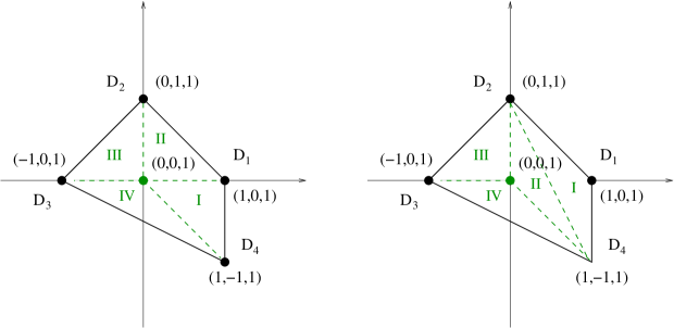
Figure 6: Two triangulation for the toric diagram of $Y^{2,1}$. The internal point $(0,0,1)$ has been blown up. One line and four planes have been added to the original fan. There are four maximal cones and corresponding fixed points, denoted I,II,III and IV.

The fan of the original variety $X$ consists of a single maximal cone, with a set of edges, or one-dimensional cones, $\Sigma(1)$ whose generators $n_{i}$ are not linearly independent in $\mathbb{Z}^{3}$. The resolutions of $X$ consist of all the possible subdivisions of the fan in smaller three dimensional cones $\sigma_{I}$. The new variety $\tilde{X}$ is still a Calabi-Yau if all the minimal generators $n_{i}$ of the one-dimensional cones lie on a plane. This process looks like a triangulation of the toric diagram. If each three-dimensional cone is generated by linearly independent primitive vectors, the variety is smooth. The smooth Calabi-Yau resolutions of $X$ thus consist of all the triangulation of the toric diagram which cannot be further subdivided. Each three dimensional cone $\sigma_{I}$ is now a copy of $\mathbb{C}^{3}$ and the smooth variety $\tilde{X}$ is obtained by gluing all these $\mathbb{C}^{3}$ according to the rules of the fan. $T^{3}$ acts on each $\sigma_{I}$ in a simple way: the three weights of the $T^{3}$ action on a copy of $\mathbb{C}^{3}$ are just given by the primitive inward normal vectors $m_{I}^{\lambda}$ to the three faces of $\sigma_{I}$. Notice that each $\sigma_{I}$ contains exactly one fixed point of $T^{3}$ (the origin in the copy of $\mathbb{C}^{3}$) with weights given by the vectors $m_{I}^{\lambda}$.

The line bundles on $\tilde{X}$ are given by $\tilde{D}=\sum_{i}c_{i}D_{i}$ where the index $i$ runs on the set of one-dimensional cones $\tilde{\Sigma}(1)$, which is typically bigger than the original $\Sigma(1)$. Indeed, each integer internal point of the toric diagram gives rise in the resolution $\tilde{X}$ to a new divisor. The space of sections of $\tilde{D}$ are still determined by the integral points of the polytope

$$\tilde{P}_{D}=\{u\in M_{\mathbb{R}}|<u,n_{i}>\,\geq\,-c_{i}\,,\,\,\forall i\in\tilde{\Sigma}(1)\}$$ (6.5)

It is important for our purposes that each maximal cone $\sigma_{I}$ determines a integral point $m_{I}^{0}\in M$ as the solution of this set of three equations:

$$<m_{I}^{0},n_{i}>=-c_{i},\,\,\,n_{i}\in\sigma_{I},$$ (6.6)

In a smooth resolution $\tilde{X}$ this equation has always integer solution since the three generators $n_{i}$ of $\sigma_{I}$ are a basis for $\mathbb{Z}^{3}$. As shown in [44], $m_{I}^{0}$ is the charge of the local equation for the divisor $\tilde{D}$ in the local patch $\sigma_{I}$. It is therefore the weight of the $T^{3}$ action on the fiber of ${\cal O}(D)$ over the fixed point contained in $\sigma_{I}$.

The strategy for computing $Z_{D}$ is therefore the following. We smoothly resolve $X$ and find a divisor $\tilde{D}=\sum_{i}c_{i}D_{i}$ by assigning values $c_{i}$ to the new one-dimensional cones in $\tilde{\Sigma}(1)$ that satisfies the two conditions

• It has the same space of sections, $H^{0}(\tilde{X},{\cal O}(\tilde{D}))=H^{0}(X,{\cal O}(D))$. Equivalently, the polytope $\tilde{P}_{D}$ has the same integer points of $P_{D}$.

• It has vanishing higher cohomology $H^{i}(\tilde{X},{\cal O}(\tilde{D}))=0,i\geq 1$. As shown in [44] this is the case if there exist integer points $m_{I}^{0}\in M$ that satisfy the convexity condition

  $$<m_{I}^{0},n_{i}> = -c_{i},\,\,\,n_{i}\in\sigma_{I}$$

  $$<m_{I}^{0},n_{i}> \geq -c_{i},\,\,\,n_{i}\notin\sigma_{I}$$ (6.7)

There are many different smooth resolution of $X$, corresponding to the possible complete triangulation of the toric diagram. It is shown in the Appendix B that we can always find a compatible resolution $\tilde{X}$ and a minimal choice of $c_{i}$ that satisfy the two given conditions.

The function $Z_{D}$ is then given as

$$Z_{D}=\sum_{P_{I}}\frac{q^{m_{I}^{0}}}{\prod_{\lambda=1}^{3}(1-q^{m_{I}^{\lambda}})}$$ (6.8)

where in the toric case for every fixed point $P_{I}$ there is a maximal cone $\sigma_{I}$, $m_{I}^{\lambda}$ are the three inward primitive normal vectors of $\sigma_{I}$ and $m_{I}^{0}$ are determined by equation (6.7). This formula can be conveniently generalized to the case where the fixed points are not isolated but there are curves or surfaces fixed by the torus action.

We finish this Section with two comments. The first is a word of caution. Note that if we change representative for a divisor in its equivalence class ($c_{i}\sim c_{i}+<M,n_{i}>$) the partition function $Z_{D}$ is not invariant, however it is just rescaled by a factor $q^{M}$.

The second comment concerns toric cones. For toric CY cones there is an alternative way of computing the partition functions $Z_{D}$ by expanding the homogeneous coordinate ring of the variety according to the decomposition (4.7). Since the homogeneous coordinate ring is freely generated by the $x_{i}$, its generating function is simply given by

$$\frac{1}{\prod_{i=1}^{d}(1-x_{i})}\,.$$

By expanding this function according to the grading given by the $(\mathbb{C}^{*})^{d-3}$ torus action we can extract all the $Z_{D}$. This approach will be discussed in detail in a future publication [42].

6.2 Examples

6.2.1 The conifold

The four primitive generators for the one dimensional cones of the conifold are $\{(0,0,1),(1,0,1),(1,1,1),(0,1,1)\}$ and we call the associated divisors $D_{1},D_{2},D_{3}$ and $D_{4}$ respectively. They satisfy the equivalence relations $D_{1}\sim D_{3}\sim-D_{2}\sim-D_{4}$. There is only one baryonic symmetry under which the four homogeneous coordinates transform as

$$(x_{1},x_{2},x_{3},x_{4})\sim(x_{1}\mu,x_{2}/\mu,x_{3}\mu,x_{4}/\mu)$$ (6.9)

The conifold case is extremely simple in that the chiral fields of the dual gauge theory are in one-to-one correspondence with the homogeneous coordinates: $(x_{1},x_{2},x_{3},x_{4})\sim(A_{1},B_{1},A_{2},B_{2})$. Recall that the gauge theory is $SU(N)\times SU(N)$ with chiral fields $A_{i}$ and $B_{p}$ transforming as $(N,\bar{N})$ and $(\bar{N},N)$ and as $(2,1)$ and $(1,2)$ under the enhanced $SU(2)^{2}$ global flavor symmetry.

The two possible resolutions for the conifold are presented in Figure 7.

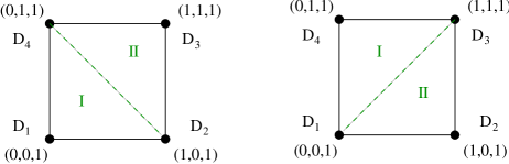
Figure 7: The two resolutions for the conifold. No internal points have been blown up. In each case, one line have been added to the original fan; there are two maximal cones and corresponding fixed points, denoted I,II.

We first compute the partition function for the divisor $D_{1}$ using the resolution on the left hand side of the figure. Regions $I$ and $II$ correspond to the two maximal cones in the resolution and, therefore, to the two fixed points of the $T^{3}$ action. Denote also $q=(q_{1},q_{2},q_{3})$. Using the prescriptions given above, we compute the three primitive inward normals to each cone and the weight of the $T^{3}$ action on the fiber. It is manifest that the conditions required in equation (6.7) are satisfied.

$${\rm Region\,I}\qquad m_{I}^{\lambda}=\{((1,0,0),(0,1,0),(-1,-1,1)\}\qquad m_{I}^{0}=(1,1,-1)$$

$${\rm Region\,II}\qquad m_{II}^{\lambda}=\{(0,-1,1),(-1,0,1),(1,1,-1)\}\qquad m_{II}^{0}=(0,0,0)$$

$$Z_{D_{1}}=\frac{q_{1}(q_{2}-q_{3})+q_{3}-q_{2}q_{3}}{(1-q_{1})(1-q_{2})(1-q_{3}/q_{1})(1-q_{3}/q_{2})q_{3}}$$ (6.10)

For simplicity, let us expand $Z_{D_{1}}$ along the direction of the Reeb vector $(3/2,3/2,3)$ by putting $q_{1}=q_{2}=q,q_{3}=q^{2}$. This corresponds to count mesonic excitations according to their R-charge, forgetting about the two $U(1)^{2}$ flavor indices.

$$Z_{D_{1}}=\frac{2}{(1-q)^{3}}=\sum_{n=0}^{\infty}(n+1)(n+2)q^{n}=2+6q+12q^{2}+...$$ (6.11)

This counting perfectly matches the list of operators in the gauge theory. In the sector of Hilbert space with baryonic charge $+1$ we find the operators (3.2)

$$A_{i}\,,\qquad A_{i}B_{p}A_{j}\,,\qquad A_{i}B_{p}A_{j}B_{q}A_{k}\,,\qquad....$$ (6.12)

The F-term equations $A_{i}B_{p}A_{j}=A_{j}B_{p}A_{i}$, $B_{p}A_{i}B_{q}=B_{q}A_{i}B_{p}$ guarantee that the $SU(2)\times SU(2)$ indices are totally symmetric. The generic operator is then of the form $A(BA)^{n}$ transforming in the $(n+2,n+1)$ representation of $SU(2)\times SU(2)$ thus exactly matching the $q^{n}$ term in $Z_{D_{1}}$. The R-charge of the operators in $Z_{D_{1}}$ is accounted by the exponent of $q$ by adding the factor $q^{\sum c_{i}R_{i}}=q^{1/2}$ which is common to all the operators in this sector (cfr. equation (4.2)). The result perfectly matches with the operators $A(BA)^{n}$ since the exact R-charge of $A_{i}$ and $B_{i}$ is $1/2$. We could easily include the $SU(2)^{2}$ charges in this counting.

Analogously, we obtain for $Z_{D_{3}}$

$$Z_{D_{3}}=\frac{q_{1}(q_{2}-q_{3})+q_{3}-q_{2}q_{3}}{(1-q_{1})(1-q_{2})(q_{1}-q_{3})(q_{2}-q_{3})}=q_{3}Z_{D_{1}}/(q_{2}q_{1})$$ (6.13)

Since $D_{1}\sim D_{3}$ the polytope $P_{D_{3}}$ is obtained by $P_{D_{1}}$ by a translation and the the two partition functions $Z_{D_{1}}$ and $Z_{D_{3}}$ are proportional. Finally, the partition functions for $D_{2}$ and $D_{4}$ are obtained by choosing the resolution in the right hand side of figure 7, for which is possible to satisfy the convexity condition (6.7)

$$Z_{D_{2}} = \frac{q_{2}(q_{1}+q_{2}-q_{1}q_{2}-q_{3})}{(1-q_{1})(1-q_{2})(q_{1}-q_{3})(q_{2}-q_{3})}$$

$$Z_{D_{4}} = \frac{q_{1}(q_{1}+q_{2}-q_{1}q_{2}-q_{3})}{(1-q_{1})(1-q_{2})(q_{1}-q_{3})(q_{2}-q_{3})}=q_{1}Z_{D_{2}}/q_{2}$$ (6.14)

6.2.2 Other examples: $Y^{p,q}$, delPezzo and $L^{p,q,r}$

In this Section we give other examples of partition functions $Z_{D}$ considering the $Y^{p,q}$, the delPezzo and $L^{p,q,r}$ manifolds.

The $Y^{p,q}$ toric diagram has four vertices and one baryonic charge. The dual gauge theory has an $SU(2)\times U(1)$ flavor symmetry. We consider the simplest example, $Y^{2,1}$. The fan for $Y^{2,1}$ has four primitive generators $\{(1,0,1),(0,1,1),(-1,0,1),(1,-1,1)\}$. The equivalence relations among divisors give $D_{2}\sim D_{4}\sim-2D_{3}$ and $D_{1}=3D_{3}$ and the corresponding homogeneous coordinates scale as

$$(x_{1},x_{2},x_{3},x_{4})\sim(x_{1}\mu^{3},x_{2}/\mu^{2},x_{3}\mu,x_{4}/\mu^{2})$$ (6.15)

under the baryonic symmetry.

There are two different completely smooth resolutions that are presented in Figure 6. The toric diagram has one internal point; the corresponding four cycle is blown up in each smooth resolution of the cone and introduces a new divisor $D_{5}$. In each resolution there are four fixed points for the action of $T^{3}$.

To compute the partition functions we need to chose a resolution and the number $c_{5}$ that satisfy the convexity condition (6.7). The partition function for $Z_{D_{3}}$ can be computed by using the resolution on the left hand side in the figure and the number $c_{5}=0$.

$${\rm Region\,I}\qquad m_{I}^{\lambda}=\{((-1,0,1),(0,-1,0),(1,1,0)\}\qquad m_{I}^{0}=(0,0,0)$$

$${\rm Region\,II}\qquad m_{II}^{\lambda}=\{((-1,-1,1),(0,1,0),(1,0,0)\}\qquad m_{II}^{0}=(0,0,0)$$

$${\rm Region\,III}\qquad m_{III}^{\lambda}=\{(1,-1,1),(0,1,0),(-1,0,0)\}\qquad m_{III}^{0}=(1,0,0)$$

$${\rm Region\,IV}\qquad m_{IV}^{\lambda}=\{(1,2,1),(0,-1,0),(-1,-1,0)\}\qquad m_{IV}^{0}=(1,1,0)$$

$$Z_{D_{3}}=\frac{-q_{3}^{2}+q_{2}^{2}(q_{1}^{2}q_{3}-q_{3}^{2}+q_{1}(1+q_{3}-q_{3}^{2}))-q_{2}(-1+q_{3}+q_{3}^{2}-q_{1}-q_{1}q_{3}+q_{1}q_{3}^{2})}{(1-q_{3}/(q_{1}q_{2}))(1-q_{3}/q_{1})(q_{2}-q_{1}q_{3})(1-q_{1}q_{2}^{2}q_{3})}$$

$Z_{D_{3}}$ can be expanded using the geometric series by setting $q_{3}=qq_{1}q_{2}$. It is immediate to verify that the first terms in the expansion $Z_{D_{3}}=1+q_{1}+q_{1}q_{2}+q(q_{2}+1+q_{1}+...)+...$ exactly match the list of field theory operators given in Section 5 (cfr Table 1).

The partition functions for the other three elementary divisors can be computed in a similar way. In order to satisfy the convexity condition we use the resolution on the left of figure 6 for $D_{2}$ and $D_{4}$ and the resolution on the right for $D_{1}$. In all cases we can safely put $c_{5}=0$.

$$Z_{D_{1}}=\frac{q_{1}^{2}q_{2}^{2}+q_{2}(1+q_{1}^{2}(1+(1+q_{1})(q_{2}+q_{2}^{2})))q_{3}-q_{1}(1+(1+q_{1})(q_{2}+q_{2}^{2}+q_{2}^{3}))q_{3}^{2}}{(q_{1}q_{2}-q_{3})(q_{1}-q_{3})(q_{2}-q_{1}q_{3})(1-q_{1}q_{2}^{2}q_{3})}$$

$$Z_{D_{2}}=\frac{q_{1}^{2}q_{2}^{2}q_{3}-q_{1}^{2}q_{2}^{2}q_{3}^{2}-q_{3}(q_{2}+(1+q_{2}+q_{2}^{2})q_{3})+q_{1}(1+q_{2})(q_{3}+q_{2}+q_{2}^{2}q_{3}-q_{2}q_{3}^{2})}{(q_{1}q_{2}-q_{3})(1-q_{3}/q_{1})(q_{2}-q_{1}q_{3})(1-q_{1}q_{2}^{2}q_{3})}$$

$$Z_{D_{4}}=q_{2}Z_{D_{2}}$$

The proportionality of $Z_{D_{4}}$ and $Z_{D_{2}}$ follows from the equivalence $D_{2}\sim D_{4}$.

Similarly, one can compute the partition functions for the other $Y^{p,q}$ manifolds and, more generally, for the $L^{p,q,r}$ manifolds which correspond to the most general toric diagram with four external points. The flavor symmetry for $L^{p,q,r}$ is $U(1)^{2}$ and, for smooth manifolds, there is exactly one baryonic symmetry. The number of internal points increases with $p,q,r$ thus making computations more involved. As an example, we present the partition function for the $D_{4}$ divisor in $L^{1,5,2}$. We refer to Figure 8 for notations and the choice of a compatible resolution.

$$Z_{D_{4}} = \frac{P(q_{1},q_{2},q_{3})}{(1-q_{2})(1-q_{1}^{4}q_{2})(q_{1}-q_{3})(q_{1}^{3}q_{2}^{2}-q_{3}^{5})}$$

$$P(q_{1},q_{2},q_{3}) = q_{1}q_{2}(q_{1}^{6}q_{2}^{2}-q_{3}^{5}-q_{1}q_{3}^{5}-q_{1}^{2}q_{3}^{2}(-1+q_{2}-q_{3}+q_{2}q_{3}+q_{3}^{3})$$ (6.16)

$$+ q_{1}^{5}q_{2}(q_{3}(1+q_{3})-q_{2}(-1+q_{3}+q_{3}^{2}))+q_{1}^{4}(-q_{2}^{2}q_{3}+q_{3}^{4}+q_{2}(1+q_{3}-q_{3}^{4}))$$

$$+ q_{1}^{3}(q_{3}^{3}+q_{3}^{4}-q_{3}^{5}-q_{2}(-1+q_{3}^{3}+q_{3}^{4})))$$

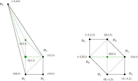
Figure 8: $L^{1,5,2}$ and $dP_{3}$. On the left: a compatible resolution for the $D_{4}$ partition function of $L^{1,5,2}$, with six fixed points. On the right: a compatible resolution for the $D_{2}$ partition function for $dP_{3}$, with six fixed points. In both cases, one can safely choose the $c_{i}$ of the extra divisors equal to zero.

Finally, we give an example based on the $dP_{3}$ manifolds, whose toric diagram has six external points and thus three different baryonic symmetries. Once again we refer to Figure 8 for notations.

$$Z_{D_{2}}=\frac{P(q_{1},q_{2},q_{3})}{(q_{1}-q_{3})(1-q_{3}/q_{2})(q_{3}-q_{1}q_{2})(1-q_{1}q_{3})(1-q_{2}q_{3})(1-q_{1}q_{2}q_{3})}$$

$$P(q_{1},q_{2},q_{3})=(q_{2}+q_{1}(1+2q_{2}+q_{1}(1+q_{2})(1+q_{2}(1+q_{1}+q_{2}))))q_{3}^{2}$$

$$-(1+q_{1}((1+q_{2})^{2}+q_{1}(1+q_{2})(1+2q_{2})+q_{1}^{2}q_{2}(1+q_{2}+q_{2}^{2})))q_{3}^{3}$$

$$+q_{1}(1+(1+q_{1})q_{2}(1+q_{1}q_{2}))q_{3}^{4}-q_{1}^{2}q_{2}-q_{1}q_{2}(q_{1}+q_{2})q_{3}$$

Following this procedure one is able to compute the partition function $Z_{D}$ for every divisor of a generic $CY$ conical toric singularity.

6.3 The partition function for BPS baryonic operators

The BPS baryonic states in a sector of the Hilbert space associated with the divisor $D$ are obtained from the $h_{m}$ by considering the N-fold symmetrized combinations $|h_{m_{1}},....,h_{m_{N}}>$. The partition function $Z_{D,N}$ for BPS baryon is obtained from $Z_{D}$ by solving a combinatorial problem [30, 33].

Given $Z_{D}$ as sum of integer points in the polytope $P_{D}$

$$Z_{D}(q)=\sum_{m\in P_{D}\cap M}q^{m}$$ (6.17)

the generating function $G_{D}(p,q)$ for symmetrized products of elements in $Z_{D}$ is given by

$$G_{D}(p,q)=\prod_{m\in P_{D}\cap M}\frac{1}{1-pq^{m}}=\sum_{N=0}^{\infty}p^{N}Z_{D,N}(q)$$ (6.18)

This formula is easy to understand: if we expand $(1-pq^{m})^{-1}$ in geometric series, the coefficient of the term $p^{k}$ is given by all possible products of $k$ elements in $P_{D}$, and this is clearly a $k$-symmetric product.
It is easy to derive the following relation between $Z_{D}(q)$ and $G_{D}(p,q)$

$$G_{D}(p,q)=e^{\sum_{k=1}^{\infty}\frac{p^{k}}{k}Z_{D}(q^{k})}$$ (6.19)

In the case we have computed $Z_{D}(q)$ in terms of the fixed point data of a compatible resolution as in equation (6.8)

$$Z_{D}(q)=\sum_{I}\frac{q^{m_{I}^{0}}}{\prod_{\lambda=1}^{3}(1-q^{m_{I}^{\lambda}})}=\sum_{I}\sum_{s_{I}^{1},s_{I}^{2},s_{I}^{3}}q^{m_{I}^{0}}q^{\sum_{\lambda=1}^{3}s_{I}^{\lambda}m_{I}^{\lambda}}$$

formula (6.19) allows, with few algebraic manipulation, to write the generating function as follows

$$G_{D}(p,q)=\prod_{P_{I}}\prod_{s_{I}^{\lambda}=0}^{\infty}\frac{1}{1-pq^{m_{I}^{0}}q^{\sum_{\lambda=1}^{3}s_{I}^{\lambda}m_{I}^{\lambda}}}$$ (6.20)

We are eventually interested in the case of BPS baryonic operators associated with the symmetrized elements $|h_{m_{1}},....,h_{m_{N}}>$, and thus to the $N$-fold symmetric partition function:

$$Z_{D,N}(q)\equiv\frac{1}{N!}\frac{\partial^{N}G_{D}(p,q)}{\partial p^{N}}\Big{|}_{p=0}$$ (6.21)

Thanks to $G_{D}(0,q)=1$ (see eq. (6.19)) we can easily write $Z_{D,N}$ in function of $Z_{D}$. For example we have:

$$Z_{D,1}(q)=Z_{D}(q)$$

$$Z_{D,2}(q)=\frac{1}{2}(Z_{D}(q^{2})+Z_{D}^{2}(q))$$

$$Z_{D,3}(q)=\frac{1}{6}(2Z_{D}(q^{3})+3Z_{D}(q^{2})Z_{D}(q)+Z_{D}^{3}(q))$$

Once we know $Z_{D}$ for a particular baryonic sector of the $BPS$ Hilbert space it is easy to write down the complete partition function $Z_{D,N}$.

7 Volumes of divisors

One of the predictions of the AdS/CFT correspondence for the background $AdS_{5}\times H$ is that the volume of $H$ is related to the central charge $a$ of the CFT, and the volumes of the three cycles wrapped by the D3-branes are related to the R-charges of the corresponding baryonic operators [4, 37]. We already used this information in formula (4.6). To many purposes, it is useful to consider the volumes as functions of the Reeb Vector $b$. Recall that each Kähler metric on the cone, or equivalently a Sasakian structure on the base $H$, determines a Reeb vector $b=(b_{1},b_{2},b_{3})$ and that the knowledge of $b$ is sufficient to compute all volumes in $H$ [17]. Denote with $\rm{Vol}_{H}(b)$ the volume of the base of a Kähler cone with Reeb vector $b$. The Calabi-Yau condition $c_{1}(X)$ requires $b_{3}=3$ [17]. As shown in [17, 35], the Reeb vector $\bar{b}$ associated with the Calabi-Yau metric can be obtained by minimizing the function $\rm{Vol}_{H}(b)$ with respect to $b=(b_{1},b_{2},3)$. This volume minimization is the geometrical counterpart of a-maximization in field theory [51]; the equivalence of a-maximization and volume minimization has been explicitly proven for all toric cones in [19] and for a class a non toric cones in [28]. For each Reeb vector $b=(b_{1},b_{2},b_{3})$ we can also define the volume of the three cycle obtained by restricting a divisor $D$ to the base, $\rm{Vol}_{D}(b)$. We can related the value $\rm{Vol}_{D}(\bar{b})$ at the minimum to the exact R-charge of the lowest dimension baryonic operator associated with the divisor $D$ [4, 37] as in formula (4.6).

All the geometrical information about volumes can be extracted from the partition functions. The relation between the character $Z_{\cal{O}}(q)$ for holomorphic functions on $C(H)$ and the volume of $H$ was suggested in [52] and proved for all Kähler cones in [35]. If we define $q=(e^{-b_{1}t},e^{-b_{2}t},e^{-b_{3}t})$, we have [52, 35]

$$\rm{Vol}_{H}(b)=\pi^{3}\lim_{t\rightarrow 0}t^{3}Z_{\cal{O}}(e^{-bt})$$ (7.1)

This formula can be interpreted as follows: the partition function $Z_{\cal{O}}(q)$ has a pole for $q\rightarrow 1$, and the order of the pole - three - reflects the complex dimension of $C(H)$ while the coefficient is related to the volume of $H$.

Here we propose that, similarly, the partition functions $Z_{D}$ contain the information about the three-cycle volumes $\rm{Vol}_{D}(b)$. Indeed we suggest that, for small $t$ ,

$$\frac{Z_{D}(e^{-bt})}{Z_{\cal{O}}(e^{-bt})}\sim 1+t\frac{\pi\rm{Vol}_{D}(b)}{2\rm{Vol}_{H}(b)}+...$$ (7.2)

Notice that the leading behaviour for all partition functions $Z_{D}$ is the same and proportional to the volume of $H$; for $q\rightarrow 1$ the main contribution comes from states with arbitrarily large dimension and it seems that states factorized in a minimal determinant times gravitons dominate the partition function. The proportionality to $\rm{Vol}_{H}$ is then expected by the analogy with giant gravitons probing the volume of $H$. The subleading term of order $1/t^{2}$ in $Z_{D}$ then contains information about the dimension two complex divisors. Physically it is easy to understand that $Z_{D}$ contains the information about the volumes of the divisors. We can think at $Z_{D}$ as a semiclassical parametrization of the holomorphic non-trivial surfaces in $X$, with a particular set of charges related to $D$; while $Z_{\mathcal{O}}$ parametrizes the set of trivial surfaces in $X$. Thinking in this way it is clear that both know about the volume of the compact space, but only $Z_{D}$ has information on the volumes of the non-trivial three cycles.

For divisors $D$ associated with elementary fields we can rewrite equation (7.2) in a simple and suggestive way in terms of the R-charge, or dimension, of the elementary field (see equation (4.6))

$$\frac{Z_{D}(e^{-bt})}{Z_{\cal{O}}(e^{-bt})}\sim 1+t\frac{3R_{D}(b)}{2}+...=1+t\Delta(b)+...$$ (7.3)

As a check of formula (7.2), we can expand the partition functions for the conifold computed in the previous Section

$$\frac{Z_{D_{i}}}{Z_{\cal{O}}}\sim(1+\frac{(b_{1}-b_{3})(b_{2}-b_{3})t}{b_{3}},1+\frac{(b_{1}b_{3}-b_{1}b_{2})t}{b_{3}},1+\frac{b_{1}b_{2}t}{b_{3}},1+\frac{(b_{2}b_{3}-b_{1}b_{2})t}{b_{3}})$$

and compare it with the formulae in [17]

$$\rm{Vol}_{D_{i}}(b)=\frac{2\pi^{2}\det\{n_{i-1},n_{i},n_{i+1}\}}{\det\{b,n_{i-1},n_{i}\}\det\{b,n_{i},n_{i+1}\}}\,,\qquad\rm{Vol}_{H}(b)=\frac{\pi}{6}\sum_{i=1}^{d}\rm{Vol}_{D_{i}}(b)$$ (7.4)

One can perform similar checks for $Y^{2,1}$ and the other cases considered in the previous section, with perfect agreement. A sketch of a general proof for formula (7.2) is given in the Appendix A.

We would like to notice that, by expanding equation (6.8) for $q=e^{-bt}\rightarrow 1$ and comparing with formula (7.2), we are able to write a simple formula for the volumes of divisors in terms of the fixed point data of a compatible resolution

$$\rm{Vol}_{D}(b)=2\pi^{2}\sum_{P_{I}}\frac{(-m_{I}^{0},b)}{\prod_{\lambda=1}^{3}(m_{I}^{\lambda},b)}$$ (7.5)

This formula can be conveniently generalized to the case where the fixed points are not isolated but there are curves or surfaces fixed by the torus action.

The previous formula is not specific to toric varieties. It can be used whenever we are able to resolve the cone $C(H)$ and to reduce the computation of $Z_{D}$ to a sum over isolated fixed points (and it can be generalized to the case where there are fixed submanifolds). As such, it applies also to non toric cones. The relation between volumes and characters may give a way for computing volumes of divisors in the general non toric case, where explicit formulae like (7.4) are not known.

8 Conclusion and Outlook

In this paper we proposed a general procedure to construct partition functions counting both baryonic and non baryonic $BPS$ operators of a field theory dual to a toric geometry. We also explained how one can extract the volumes of the three cycles from the partition functions. It would be interesting to understand better the counting of multiplicity, and to find a way to write down a complete partition function for the $BPS$ gauge invariant scalar operators [42].

Our computation is done on the supergravity side, and it is therefore valid at strong coupling. Similarly to the partition function for BPS mesonic operators [30, 32, 33], we expect to be able to extrapolate the result to finite value for the coupling.

It would be also interesting to understand better the non toric case. Most of the discussions in this paper apply to this case as well. The classical configurations of BPS D3 branes wrapping a divisor $D$ are still parameterized by the generic section of $H^{0}(X,{\cal O}(D))$ and Beasley’s prescription for constructing the BPS Hilbert space is unchanged. The partition function $Z_{D}(q)$ can be still defined, with the only difference that $q\in T^{k}$ with $k$ strictly less than three. $Z_{D}(q)$ can be still computed by using the index theorem as explained in Section 6 and the relation between $Z_{D}(q)$ and the three cycles volumes should be still valid. In particular, when $X$ has a completely smooth resolution with only isolated fixed points for the action of $T^{k}$, formulae (6.8) and (7.5) should allow to compute the partition functions and the volume. What is missing in the non-toric case is an analogous of the homogeneous coordinates, the polytopes and the existence of a canonical smooth resolution of the cone. But this seems to be just a technical problem.

Acknowledgments

We would like to thank Amihay Hanany and Alessandro Tomasiello for useful discussions. D.F. thanks Jose D. Edelstein, Giuseppe Milanesi and Marco Pirrone for useful discussions. This work is supported in part by INFN and MURST under contract 2005-024045-004 and 2005-023102 and by the European Community’s Human Potential Program MRTN-CT-2004-005104.

Appendix A Localization formulae for the volumes of divisors

Relation (7.2) can be easily proven in the case where the Reeb action is regular, by adapting an argument in [52, 53], as refined in [35]. For a regular action, $H$ is a $U(1)$ principal bundle over a Kähler manifold $V$ and $X$ can be written as a line bundle $L\rightarrow V$. We can blow up $V$ and apply equivariant Riemann-Roch to the resulting manifold. Since the Reeb vector acts on the fibers of $L$, its fixed locus is the entire $V$ with weight $1$. We thus obtain

$$Z_{D}(q)=\int_{V}\frac{{\rm Todd}(V)Ch(D)}{1-qe^{-c_{1}(L)}}$$ (A.1)

Put $q=e^{-bt}$ in this formula. The denominator must be expanded in a formal power series of forms before taking the limit $t\rightarrow 0$

$$\frac{1}{1-qe^{-c_{1}(L)}}=\frac{1}{1-e^{-bt}}-\frac{e^{-bt}}{(1-e^{-bt})^{2}}c_{1}(L)+\frac{e^{-bt}+e^{-2bt}}{2(1-e^{-bt})^{3}}c_{1}(L)^{2}$$

Since the integral over $V$ selects forms of degree four we obtain

$$Z_{D}(q)=\frac{1}{(bt)^{3}}\int_{V}c_{1}(L)^{2}-\frac{1}{(bt)^{2}}\int_{V}c_{1}(L)\wedge{\rm Todd}(V)\wedge Ch(D)\Big{|}_{{\rm degree}\,4}+...$$

The only information we need about the Todd class is that ${\rm Todd}(V)=1+...$. We thus obtain

$$\frac{Z_{D}(q)}{Z_{\cal O}}=1-b\,t\,\frac{\int_{V}c_{1}(L)\wedge c_{1}(D)}{\int_{V}c_{1}(L)\wedge c_{1}(L)}+...$$

The volumes of $H$ and of the three cycle $D\cap H$, which are $U(1)$ fibrations over $V$ and $D\cap V$, are proportional to

$${\rm Vol}_{D}(b) \sim \int_{D}\omega_{V}=\int_{V}\omega_{V}\wedge c_{1}(D)$$

$${\rm Vol}_{H}(b) \sim \int_{V}\frac{\omega_{V}^{2}}{2}$$ (A.2)

Considering that the first Chern class of $L$ is proportional to the Kähler form $\omega_{V}$ on $V$ , we finally obtain

$$\frac{Z_{D}(q)}{Z_{\cal O}}=1+t\frac{\pi\rm{Vol}_{D}(b)}{2\rm{Vol}_{H}(b)}+...$$

Formula (7.2) could be proven for a generic Sasaki-Einstein by generalizing arguments in [35]. We only suggest a possible proof, leaving to experts the subtle task of filling mathematical details. As argued in [35], it is enough to prove (7.2) for quasi regular actions; since a rational $b\in T^{k}$ defines a Sasaki structure on $H$ with quasi regular Reeb action, formula (7.2) would be true for all rational $b$ and, therefore, for continuity, for all $b$. For a quasi regular action, $L\rightarrow V$ is an orbifold and we should use the Kawasaki-Riemann-Roch formula [54] which have extra contributions with respect to (A.1). However, for isolated orbifold singularities, the extra contributions are characteristic classes integrated over points; these contribute to $Z_{D}(q)$ only at order $1/t$ and should be irrelevant for our purposes.

It would be interesting to fully understand formula (7.2) in terms of localization. It seems that some localization theorem is at work here. Considering that the action of the Reeb field

$$\xi=\sum_{i=1}^{k}b_{i}\frac{\partial}{\partial\phi_{i}}$$

(we have chosen $k$ angular coordinates for the torus $T^{k}$ action, $k=1,2,3$) is hamiltonian, we can define the equivariantly closed form $\omega^{\xi}=\omega-H$ starting from the kähler class $\omega$ . As shown in [35], the hamiltonian for the Reeb action is $H=r^{2}/2$. Analogously we can define the equivariant first Chern class $c_{1}^{\xi}(D)$ associated with the divisor $D$. It is interesting to notice that the expression (7.5) for the volumes can be written as the integral of equivariantly characteristic classes,

$$\frac{1}{2}\int_{X}e^{\omega^{\xi}}\wedge c_{1}^{\xi}(D)=2\pi^{2}\sum_{\sigma_{I}}\frac{(-m_{I}^{0},b)}{\prod_{\lambda=1}^{3}(m_{I}^{\lambda},b)}$$ (A.3)

This equality can be proven as follows. Suppose that we have found a smooth resolution $\tilde{X}$ of the cone $X$ and a divisor $\tilde{D}$ that smoothly approach $D$ in the singular limit. We may then compute the previous integral for $\tilde{X}$ and $\tilde{D}$ and take afterwards the limit $\tilde{X}\rightarrow X$. Integrals of equivariantly closed forms, like (A.3), can be computed by using localization theorems. Indeed given an equivariantly closed form $\alpha$ and an action along a direction in $T^{k}$ ($k=1,2,3$ ) with only isolated fixed points, it can be shown that

$$\int\alpha=(2\pi)^{3}\sum_{P_{I}}\frac{\alpha|_{P_{I}}}{\prod_{\lambda=1}^{3}(m_{I}^{\lambda},b)}$$ (A.4)

where $m_{I}^{\lambda}$ are, as usual, the weights of the action of $\xi$ on the tangent space at $P_{I}$. The integral over a point $P_{I}$ takes contribution only from the forms with zero degree in the equivariant forms,

$$\omega^{\xi}\rightarrow-H(P_{I})$$

$$c_{1}^{\xi}(D)\rightarrow-\frac{(m_{I}^{0},b)}{2\pi}$$ (A.5)

where $m_{I}^{0}$ is the weight of the action on the line bundle fiber over $P_{I}$ . Taking into account that in the singular limit all the $P_{I}$s collapse to the apex of the cone where $H=0$, we finally obtain formula (A.3).

On the other hand, also the volume of the base $D\cap H$ can be written as an integral

$$\rm{Vol_{D}}(b)=\frac{1}{2}\int_{D}e^{-r^{2}/2}\,\frac{\omega^{2}}{2}=\frac{1}{2}\int_{D}e^{\omega^{\xi}}$$ (A.6)

Comparing this equation with the expression (A.3) for the volumes we find the suggestive equality

$$\int_{D}e^{\omega^{\xi}}=\int_{X}e^{\omega^{\xi}}\wedge c_{1}^{\xi}(D)\,.$$ (A.7)

concerning $T$ invariant divisors $D$. Our general expression for the volumes (7.5) (which, in case there exist smooth resolutions for $X$ with isolated fixed points, is completely equivalent to the general formula (7.2)) would be proved if we were able to prove equation (A.7). The relation between equivariant cohomology and homology seems to be not completely understood (to us at least), and we do not know under what condition the equation (A.7) is valid, even if this is probably well known to experts. A better understanding of this formula could give a simple alternative proof for (7.2).

Appendix B Convexity condition and integer counting

In this Appendix we give an alternative explanation of the formula (6.8) for computing the partition function $Z_{D}$ defined in (6.1) and we explain why there always exists a suitable resolution of $X=C(H)$ and a suitable choice of weights $\tilde{c}_{i}$ for equation (6.8). In Section 6.1 we explained how to derive this formula from the equivariant Riemann-Roch theorem. However since $Z_{D}$ counts the holomorphic sections of $\mathcal{O}(D)$ and since we know that, for toric singularities, these sections are in one to one correspondence with the integer points inside the polytope $P_{D}$, we can simply look at this problem as that of counting integer points inside a polytope, with the weights $q=(q_{1},q_{2},q_{3})$ being associated with the three cartesian coordinates: $Z_{D}=\sum_{m\in P_{D}\cap M}q^{m}$. This simple point of view allows to have a direct understanding of the counting problem.

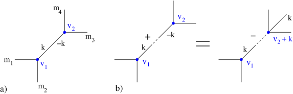
Figure 9: a) The (p,q) web for the conifold resolution corresponding to the first diagram in Figure 7. b) A pictorial description of equation (B.5).

To be concrete consider for instance the case of the conifold; let us write the character that counts integer points inside the dual fan, which is equivalent to counting holomorphic functions, or sections of the trivial bundle $\mathcal{O}$. The dual fan is generated by the four vectors:

$$m_{1}=(1,0,0)\quad m_{2}=(0,1,0)\quad m_{3}=(-1,0,1)\quad m_{4}=(0,-1,1)$$ (B.1)

all attached at the origin $n=(0,0,0)$. To compute the character we will use for instance the first resolution in Figure 7, whose corresponding (p,q) web is drawn in Figure 9 a). Let us define the vector $k=(-1,-1,1)$. We split the (p,q) web into two subwebs corresponding to region I and II respectively of the resolution in Figure 7:

$$\begin{array}[]{l@{\qquad}l@{\qquad\qquad}l}\textrm{Region I}&\{m_{1},m_{2},k\}&v_{1}=(0,0,0)\\ \textrm{Region II}&\{m_{3},m_{4},-k\}&v_{2}=(0,0,0)\end{array}$$ (B.2)

We denote with $v_{1}$ ($v_{2}$) the integer point to which the three vectors of region I (II) are attached. In this case $v_{1}=v_{2}=(0,0,0)$. Since we have completely resolved the conifold, according to [35], the character is:

$$Z_{\mathcal{O}}=\frac{1}{(1-q^{m_{1}})(1-q^{m_{2}})(1-q^{k})}+\frac{1}{(1-q^{m_{3}})(1-q^{m_{4}})(1-q^{-k})}$$ (B.3)

where as usual $q^{h}\equiv q_{1}^{h_{1}}q_{2}^{h_{2}}q_{3}^{h_{3}}$. It is simple to give an interpretation of this formula in terms of counting of integer points. Let us for instance expand the first term, associated with Region I, in equation (B.3). We get

$$\left(\sum_{i=0}^{\infty}q^{i\,m_{1}}\right)\left(\sum_{j=0}^{\infty}q^{j\,m_{2}}\right)\left(\sum_{h=0}^{\infty}q^{h\,k}\right)=\sum_{i,j,h\geq 0}q^{i\,m_{1}+j\,m_{2}+h\,k}$$ (B.4)

and this is just the partition function that counts integer points inside the cone generated by the vectors $\{m_{1},m_{2},k\}$ attached to the origin $v_{1}=(0,0,0)$. In fact each integer point inside this cone can be written in a unique way as a linear combination of $\{m_{1},m_{2},k\}$ with positive integers due to the fact that $\textrm{det}(m_{1},m_{2},k)=1$. This is equivalent to the statement that region I is a triangle with integer points with minimal area (=1/2).

Note that the cone generated by $\{m_{1},m_{2},k\}$ centered in $(0,0,0)$ strictly includes the cone generated by the four vectors $m_{i}$; this is dual to the statement that region I is included in the fan of the conifold. The second term in (B.3) exactly cancels the integer points that belong to $\{m_{1},m_{2},k\}$ but not to the cone generated by the $m_{i}$.

The important observation is that expansion (B.4) is valid in the region $\{q^{m_{1}}<1,q^{m_{2}}<1,q^{k}<1\}$. Since the second term in (B.3) contains the factor $q^{-k}$ before expanding it in the usual way we can rearrange the expression (B.3) for $Z_{\mathcal{O}}$ as

$$Z_{\mathcal{O}}=\frac{1}{(1-q^{m_{1}})(1-q^{m_{2}})(1-q^{k})}-\frac{q^{k}}{(1-q^{m_{3}})(1-q^{m_{4}})(1-q^{k})}$$ (B.5)

Now we can expand both these terms in the region: $q^{m_{i}}<1,\forall i=1,\ldots 4$ and $q^{k}<1$. The factor of $q^{k}$ in front of the second term simply translates the origin: we get the partition function that counts integer points inside the cone $\{m_{1},m_{2},k\}$ with origin $(0,0,0)$ minus the partition function that counts integer points inside the cone $\{m_{3},m_{4},k\}$ centered at the integer point $k$. Note that since $k$ is a primitive vector, along the line with direction $k$ and passing through $(0,0,0)$, the point $k$ is the first integer point after the origin $(0,0,0)$. We have thus canceled all the integer points we didn’t want to count and hence $Z_{\mathcal{O}}$ is the correct partition function. A pictorial description of equation (B.5) is given in Figure 9 b); we project the edges of the cones on the (p,q) web plane (first two coordinates). The reader should try to imagine the process in three dimensions.

Obviously one can repeat the same process exchanging $k\leftrightarrow-k$: we expand the second term of (B.3) for $\{q^{m_{3}}<1,q^{m_{4}}<1,q^{-k}<1\}$ and rearrange the first term of (B.3); we see that the same expansion for $Z_{\mathcal{O}}$ is valid in the region $q^{m_{i}}<1,\forall i=1,\ldots 4$ and $q^{-k}<1$. Combining with the previous result, we obtain that $Z_{\mathcal{O}}$ can be expanded in the region $q^{m_{i}}<1,\forall i=1,\ldots 4$, that is only the external vectors $m_{i}$ matter. Obviously taking the second resolution for the conifold of Figure 7 one arrives at the same function $Z_{\mathcal{O}}$.

It is easy to see now how to write the partition function that counts integer points inside a polytope obtained by moving the origins $v_{1}$ and $v_{2}$ of the two cones at arbitrary, non coincident, points. We obtain:

$$\frac{q^{v_{1}}}{(1-q^{m_{1}})(1-q^{m_{2}})(1-q^{k})}+\frac{q^{v_{2}}}{(1-q^{m_{3}})(1-q^{m_{4}})(1-q^{-k})}$$ (B.6)

since the factors $q^{v_{J}}$ are simply translating the origins. For instance in the case of $Z_{D_{1}}$ in Section 6.2.1 we had $v_{1}=(1,1,-1)$ and $v_{2}=(0,0,0)$, there called $m^{0}_{I}$ and $m^{0}_{II}$. This is another explanation of formula (6.8).

It is not difficult to generalize this example to all cases we are interested in. Suppose you have a rational convex polytope in $\mathbb{R}^{3}$ with integer vertices; call $m^{0}_{J}$ its vertices and $m_{J}^{\lambda}$ the edges attached to each vertex $m^{0}_{J}$. We normalize the $m_{J}^{\lambda}$ to primitive integer vectors (all exiting from the vertex $m^{0}_{J}$). At each vertex suppose that the infinite cone generated by the $m_{J}^{\lambda}$ is of Calabi-Yau type (meaning that the dual cone has generators lying on the plane $z=1$); as we will see later this is our case. Then one can easily compute the partition function $Z_{J}(q)$ that counts integer points inside the infinite cone with vertex in $(0,0,0)$ generated by the vectors $m_{J}^{\lambda}$, with fixed $J$, for instance by taking any resolution of the associated fan. Repeating the trick above, it is easy to see that the partition function that counts integer points inside the original polytope is given by the sum $\sum_{J}q^{m^{0}_{J}}Z_{J}(q)$ over all vertices $J$ of the polytope.

Now we go back to the original problem of Section 6.1. To fix the notation, let $c_{i}$ be the generic integer weights assigned to each vertex $n_{i}$ of a toric diagram that define the bundle: $\mathcal{O}(\sum_{i}c_{i}D_{i})$, $i\in\Sigma(1)$; where $\Sigma(1)$ is the set of vertices $n_{i}=(y_{i},z_{i},1)$ of the toric diagram. Let $P_{D}$ the polytope in $\mathbb{R}^{3}$ defined by the equations:

$$P_{D}=\{m\in\mathbb{R}^{3}|\langle m,n_{i}\rangle+c_{i}\geq 0,\,\forall i\in\Sigma(1)\}$$ (B.7)

One can compute the intersections of these planes and reconstruct the edges and the vertices of $P_{D}$. There is a plane for each vertex $V_{i}$. An example is reported in Figure 10 a): in this case the polytope has 7 planes and 4 vertices $v_{J}$. In general $P_{D}$ is convex and has rational edges, however its vertices are only rational and may not be integer. Therefore we define another convex polytope $\tilde{P}_{D}$ as the convex hull of all integer points inside $P_{D}$. Therefore $\tilde{P}_{D}\subseteq P_{D}$ and all integer points in $P_{D}$ belong also to $\tilde{P}_{D}$: the original problem is reduced to the problem of counting integer points inside $\tilde{P}_{D}$.

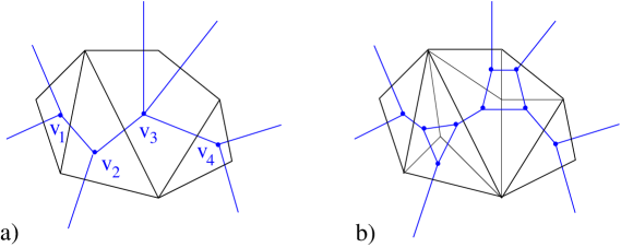
Figure 10: a) Edges of the polytope $P_{D}$ projected on the (p,q) web plane (in blue) and dual resolved toric diagram (in black). b) The same picture for $\tilde{P}_{D}$.

It is easy to see that $\tilde{P}_{D}$ can be alternatively described by adding equations to those defining $P_{D}$ (B.7), since the infinite edges of $P_{D}$, being described by rational equations, pass through integer points. An example is reported in Figure 10 b), where we draw projected on the (p,q) web plane the edges of $\tilde{P}_{D}$ corresponding to the polytope $P_{D}$ in Figure 10 a). Note that besides the 7 infinite pieces of planes delimiting $P_{D}$ we have added two finite pieces of planes; in the dual description this corresponds to refine the resolution of the toric diagram by adding two internal points $\tilde{n}_{i}$, the perpendiculars to the two planes.

An important fact is that the resolution we need to describe $\tilde{P}_{D}$ is again Calabi-Yau, meaning that the only planes we need to add to equations (B.7) are those with perpendiculars $\tilde{n}_{i}\in\tilde{\Sigma}(1)$ where $\tilde{\Sigma}(1)$ is the set of integer vectors $\tilde{n}_{i}$ lying on the plane of the toric diagram and inside the toric diagram. Consider for any integer vector $\tilde{n}_{i}\in\tilde{\Sigma}(1)$ the plane $\langle m,\tilde{n}_{i}\rangle+a=0$; by varying $a$ it is easy to see that for large positive $a$ the plane does not intersect $\tilde{P}_{D}$; hence there is a maximal value of $a$ for which the plane has a non empty intersection with the closed polytope $\tilde{P}_{D}$. Define $\tilde{c}_{i}$ such value for $a$. Obviously if $\tilde{n}_{i}=n_{i}$ coincides with an external vertex of the toric diagram we obtain for $\tilde{c}_{i}$ the original value $c_{i}$. Note that all $\tilde{c}_{i}$ are integers since $\tilde{P}_{D}$ has integer vertices. Now define the polytope $Q$:

$$Q=\{m\in\mathbb{R}^{3}|\langle m,\tilde{n}_{i}\rangle+\tilde{c}_{i}\geq 0,\,\forall i\in\tilde{\Sigma}(1)\}$$ (B.8)

with the $\tilde{c}_{i}$ defined as before. It is not difficult to prove that $Q=\tilde{P}_{D}$. In fact from the definitions we straightforwardly obtain that: $\tilde{P}_{D}\subseteq Q\subseteq P_{D}$. Now the convex polytope $Q$ can be seen as the convex hull of its vertices and of the integer points along its infinite external edges. If we prove that $Q$ has integer vertices then we would prove also $Q\subseteq\tilde{P}_{D}$ since $\tilde{P}_{D}$ is the convex hull of all integer points inside $P_{D}$; and hence $Q=\tilde{P}_{D}$.

By computing the intersections of the planes in the definition (B.8) we can obtain the corresponding resolution of the toric diagram and the vertices of the polytope $Q$. For example one could obtain the resolution in Figure 10 b), where the toric diagram has been divided into 9 regions $\rho_{J}$, $I=1\ldots 9$, each corresponding to a vertex $m^{0}_{J}$ of the convex polytope $Q$. The vertex $m^{0}_{J}$ is the intersection of the planes $\langle m,\tilde{n}_{i}\rangle+\tilde{c}_{i}=0$, for all the vertices $\tilde{n}_{i}$ of the region $\rho_{J}$. If the region $\rho_{J}$ we are considering has no internal integer point, then by the Pick’s theorem [44] it is a triangle with minimal area $1/2$; call its integer vertices $\tilde{n}_{1}$, $\tilde{n}_{2}$ and $\tilde{n}_{3}$. Since for this triangle $\det(\tilde{n}_{1},\tilde{n}_{2},\tilde{n}_{3})=1$, $m^{0}_{J}$ is an integer point. Instead if the region $\rho_{J}$ has integer points inside it is easy to see from the construction of $Q$ that all the planes $\langle m,\tilde{n}_{i}\rangle+\tilde{c}_{i}=0$, for any integer $\tilde{n}_{i}$ internal to $\rho_{J}$, pass through the vertex $m^{0}_{J}$. Hence we can take any complete resolution of the region $\rho_{J}$ into minimal triangles and compute $m^{0}_{J}$ as the intersection of the planes associated to its three vertices. Hence again $m^{0}_{J}$ is integer. All minimal triangles belonging to the region $\rho_{J}$ identify the same $m^{0}_{J}$.

We just proved that $Q$ has integer vertices and hence $Q=\tilde{P}_{D}$. Since $\tilde{P}_{D}$ is Calabi-Yau, to compute the partition function $Z_{D}$ that counts its integer points we can use the method derived above:

$$Z_{D}=\sum_{\rho_{J}}q^{m^{0}_{J}}Z_{J}(q)$$ (B.9)

where as before $Z_{J}$ is the partition function counting integer points inside the cone with apex in $(0,0,0)$ generated by the edges $m^{\lambda}_{J}$ attached to vertex $m^{0}_{J}$. Moreover the partition functions $Z_{J}$ can be computed using any complete resolution of the regions $\rho_{J}$; we obtain therefore a refined resolution of the toric diagram in minimal triangles $\sigma_{I}$. The resulting partition function is just formula (6.8).

Note that there is some ambiguity in choosing the complete resolution of the toric diagram into triangles $\sigma_{I}$; however this resolution must be compatible with the starting $\rho_{J}$ resolution. To summarize we have given an alternative proof of (6.8) and we have explicitly built the integers $\tilde{c}_{i}$ associated with the internal points $\tilde{n}_{i}\in\tilde{\Sigma}(1)$. Then the equations (B.8) define a resolution $\rho_{J}$ of the toric diagram that can be further refined. Note that the two conditions given in Section 6.1 are naturally satisfied with this geometrical choice of $\tilde{c}_{i}$; in particular convexity (6.7) follows from the fact that $m^{0}_{J}$ are the vertices of $\tilde{P}_{D}$.

References

- [1] J. M. Maldacena, “The large N limit of superconformal field theories and supergravity,” Adv. Theor. Math. Phys. 2 (1998) 231 [Int. J. Theor. Phys. 38 (1999) 1113] [arXiv:hep-th/9711200].
- [2] I. R. Klebanov and E. Witten, “Superconformal field theory on threebranes at a Calabi-Yau singularity,” Nucl. Phys. B 536, 199 (1998) [arXiv:hep-th/9807080].
- [3] B. S. Acharya, J. M. Figueroa-O’Farrill, C. M. Hull and B. Spence, “Branes at conical singularities and holography,” Adv. Theor. Math. Phys. 2, 1249 (1999) [arXiv:hep-th/9808014]; D. R. Morrison and M. R. Plesser, “Non-spherical horizons. I,” Adv. Theor. Math. Phys. 3, 1 (1999) [arXiv:hep-th/9810201].
- [4] S. S. Gubser and I. R. Klebanov, “Baryons and domain walls in an N = 1 superconformal gauge theory,” Phys. Rev. D 58 (1998) 125025 [arXiv:hep-th/9808075].
- [5] J. P. Gauntlett, D. Martelli, J. Sparks and D. Waldram, “Supersymmetric AdS(5) solutions of M-theory,” Class. Quant. Grav. 21, 4335 (2004) [arXiv:hep-th/0402153]; “Sasaki-Einstein metrics on S(2) x S(3),” Adv. Theor. Math. Phys. 8, 711 (2004) [arXiv:hep-th/0403002]; “A new infinite class of Sasaki-Einstein manifolds,” Adv. Theor. Math. Phys. 8, 987 (2006) [arXiv:hep-th/0403038].
- [6] M. Cvetic, H. Lu, D. N. Page and C. N. Pope, “New Einstein-Sasaki spaces in five and higher dimensions,” Phys. Rev. Lett. 95, 071101 (2005) [arXiv:hep-th/0504225]; “New Einstein-Sasaki and Einstein spaces from Kerr-de Sitter,” arXiv:hep-th/0505223.
- [7] D. Martelli and J. Sparks, “Toric Sasaki-Einstein metrics on S**2 x S**3,” Phys. Lett. B 621, 208 (2005) [arXiv:hep-th/0505027].
- [8] D. Martelli and J. Sparks, “Toric geometry, Sasaki-Einstein manifolds and a new infinite class of AdS/CFT duals,” Commun. Math. Phys. 262, 51 (2006) [arXiv:hep-th/0411238].
- [9] S. Benvenuti, S. Franco, A. Hanany, D. Martelli and J. Sparks, “An infinite family of superconformal quiver gauge theories with Sasaki-Einstein duals,” JHEP 0506, 064 (2005) [arXiv:hep-th/0411264].
- [10] S. Benvenuti and M. Kruczenski, “From Sasaki-Einstein spaces to quivers via BPS geodesics: Lpqr,” JHEP 0604, 033 (2006) [arXiv:hep-th/0505206].
- [11] A. Butti, D. Forcella and A. Zaffaroni, “The dual superconformal theory for L(p,q,r) manifolds,” JHEP 0509, 018 (2005) [arXiv:hep-th/0505220].
- [12] S. Franco, A. Hanany, D. Martelli, J. Sparks, D. Vegh and B. Wecht, “Gauge theories from toric geometry and brane tilings,” JHEP 0601, 128 (2006) [arXiv:hep-th/0505211].
- [13] A. Brini and D. Forcella, “Comments on the non-conformal gauge theories dual to Ypq manifolds,” JHEP 0606:050,2006 [arXiv:hep-th/0603245].
- [14] M. Bertolini, F. Bigazzi and A. L. Cotrone, “New checks and subtleties for AdS/CFT and a-maximization,” JHEP 0412, 024 (2004) [arXiv:hep-th/0411249].
- [15] A. Hanany, P. Kazakopoulos and B. Wecht, “A new infinite class of quiver gauge theories,” JHEP 0508, 054 (2005) [arXiv:hep-th/0503177].
- [16] A. Hanany and K. D. Kennaway, “Dimer models and toric diagrams,” arXiv:hep-th/0503149; S. Franco, A. Hanany, K. D. Kennaway, D. Vegh and B. Wecht, “Brane dimers and quiver gauge theories,” JHEP 0601, 096 (2006) [arXiv:hep-th/0504110].
- [17] D. Martelli, J. Sparks and S. T. Yau, “The Geometric Dual of a-maximization for Toric Sasaki-Einstein Manifolds,” Commun. Math. Phys. 268, 39 (2006) [arXiv:hep-th/0503183].
- [18] S. Benvenuti and M. Kruczenski, “Semiclassical strings in Sasaki-Einstein manifolds and long operators in N = 1 gauge theories,” JHEP 0610, 051 (2006) [arXiv:hep-th/0505046].
- [19] A. Butti and A. Zaffaroni, “R-charges from toric diagrams and the equivalence of a-maximization and Z-minimization,” JHEP 0511, 019 (2005) [arXiv:hep-th/0506232].
- [20] A. Butti and A. Zaffaroni, “From toric geometry to quiver gauge theory: The equivalence of a-maximization and Z-minimization,” Fortsch. Phys. 54, 309 (2006) [arXiv:hep-th/0512240].
- [21] A. Hanany and D. Vegh, “Quivers, tilings, branes and rhombi,” arXiv:hep-th/0511063.
- [22] B. Feng, Y. H. He, K. D. Kennaway and C. Vafa, “Dimer models from mirror symmetry and quivering amoebae,” arXiv:hep-th/0511287.
- [23] S. Gubser, N. Nekrasov and S. Shatashvili, “Generalized conifolds and four dimensional N = 1 superconformal JHEP 9905 (1999) 003 [arXiv:hep-th/9811230].
- [24] E. Lopez, “A family of N = 1 SU(N)**k theories from branes at singularities,” JHEP 9902 (1999) 019 [arXiv:hep-th/9812025].
- [25] A. Hanany and A. Iqbal, “Quiver theories from D6-branes via mirror symmetry,” JHEP 0204, 009 (2002) [arXiv:hep-th/0108137].
- [26] M. Wijnholt, “Large volume perspective on branes at singularities,” Adv. Theor. Math. Phys. 7 (2004) 1117 [arXiv:hep-th/0212021].
- [27] S. Franco, A. Hanany and P. Kazakopoulos, “Hidden exceptional global symmetries in 4d CFTs,” JHEP 0407, 060 (2004) [arXiv:hep-th/0404065].
- [28] A. Butti, D. Forcella and A. Zaffaroni, “Deformations of conformal theories and non-toric quiver gauge theories,” arXiv:hep-th/0607147.
- [29] C. Romelsberger, “An index to count chiral primaries in N = 1 d = 4 superconformal field theories,” arXiv:hep-th/0510060.
- [30] J. Kinney, J. M. Maldacena, S. Minwalla and S. Raju, “An index for 4 dimensional super conformal theories,” arXiv:hep-th/0510251.
- [31] G. Mandal and N. V. Suryanarayana, “Counting 1/8-BPS dual-giants,” arXiv:hep-th/0606088.
- [32] I. Biswas, D. Gaiotto, S. Lahiri and S. Minwalla, “Supersymmetric states of N = 4 Yang-Mills from giant gravitons,” arXiv:hep-th/0606087.
- [33] S. Benvenuti, B. Feng, A. Hanany and Y. H. He, “Counting BPS operators in gauge theories: Quivers, syzygies and plethystics,” arXiv:hep-th/0608050.
- [34] D. Martelli and J. Sparks, “Dual giant gravitons in Sasaki-Einstein backgrounds,” arXiv:hep-th/0608060.
- [35] D. Martelli, J. Sparks and S. T. Yau, “Sasaki-Einstein manifolds and volume minimisation,” arXiv:hep-th/0603021.
- [36] J. McGreevy, L. Susskind and N. Toumbas, ‘Invasion of the giant gravitons from anti-de Sitter space,” JHEP 0006 (2000) 008 [arXiv:hep-th/0003075].
- [37] S. S. Gubser, “Einstein manifolds and conformal field theories,” Phys. Rev. D 59 (1999) 025006 [arXiv:hep-th/9807164].
- [38] A. Mikhailov, “Giant gravitons from holomorphic surfaces,” JHEP 0011 (2000) 027 [arXiv:hep-th/0010206].
- [39] C. E. Beasley, “BPS branes from baryons,” JHEP 0211 (2002) 015 [arXiv:hep-th/0207125].
- [40] F. Canoura, J. D. Edelstein, L. A. P. Zayas, A. V. Ramallo and D. Vaman, “Supersymmetric branes on AdS(5) x Y**(p,q) and their field theory duals,” JHEP 0603 (2006) 101 [arXiv:hep-th/0512087].
- [41] F. Canoura, J. D. Edelstein and A. V. Ramallo, “D-brane probes on L(a,b,c) superconformal field theories,” JHEP 0609 (2006) 038 [arXiv:hep-th/0605260].
- [42] D. Forcella, A. Hanany and A. Zaffaroni, hep-th/0701236; A. Butti, D. Forcella, A. Hanany, D. Vegh and A. Zaffaroni, in preparation.
- [43] D. Cox, “What is a Toric Variety?,” Comtemporary Mathematics 14M25 (1991).
- [44] W. Fulton, “Introduction to Toric Varieties”, Princeton University Press, 1993.
- [45] D. A. Cox, “The Homogeneous Coordinate Ring of a Toric Variety, Revised Version,” arXiv:alg-geom/9210008.
- [46] D. Berenstein, C. P. Herzog and I. R. Klebanov, “Baryon spectra and AdS/CFT correspondence,” JHEP 0206 (2002) 047 [arXiv:hep-th/0202150].
- [47] N. M. J. Woodhouse, Geometric Quantization, Second Ed., (Clarendon Press, Oxford, 1992).
- [48] A. Butti, “Deformations of toric singularities and fractional branes,” JHEP 0610, 080 (2006) [arXiv:hep-th/0603253].
- [49] A. Hanany, C. P. Herzog and D. Vegh, “Brane tilings and exceptional collections,” JHEP 0607, 001 (2006) [arXiv:hep-th/0602041].
- [50] M. F. Atiyah, I. M. Singer, “The index of elliptic operators III,” Ann. Math. 87, 546-604 (1968).
- [51] K. Intriligator and B. Wecht, “The exact superconformal R-symmetry maximizes a,” Nucl. Phys. B 667, 183 (2003) [arXiv:hep-th/0304128].
- [52] A. Bergman and C. P. Herzog, “The volume of some non-spherical horizons and the AdS/CFT correspondence,” JHEP 0201 (2002) 030 [arXiv:hep-th/0108020].
- [53] C. P. Herzog and J. McKernan, “Dibaryon spectroscopy,” JHEP 0308, 054 (2003) [arXiv:hep-th/0305048].
- [54] T. Kawasaki, “The Riemann-Roch theorem for complex V-manifolds” Osaka J. math. 16, 151 (1979); M. Vergne, “The equivariant index formula on orbifolds”, Duke Math. J. 82, 637 (1996).