We apply to non-critical bosonic Liouville string models, characterized by a central-charge deficit $Q$, a new non-perturbative renormalization-group technique based on a functional method for controlling the quantum fluctuations. We demonstrate the existence of a renormalization-group fixed point of Liouville string theory as $Q\to 0$, in which limit the target space-time is Minkowski and the dynamics of the Liouville field is trivial, as it neither propagates nor interacts. This calculation supports in a non-trival manner the identification of the zero mode of the Liouville field with the target time variable, up to a crucial minus sign.

1 Introduction

In non-critical strings of the type discussed in [1], one has a conformal field theory formulated in general in a non-critical number of spatial dimensions with a central charge deficit $Q$. This might either assume discrete values, as in the minimal models discussed in [1], or possibly vary continuously, as in models motivated by brane world collisions [2]. In the latter case, the central charge of the corresponding world-sheet $\sigma$ model describing string excitations on the brane and in the bulk space is proportional to some power of the relative velocity of the moving models (assuming that the collisions are adiabatic, so that perturbative string theory applies).

In general, non-equilibrium situations in string cosmology, such as those that may well have characterized the early Universe, can be described [2] at large times long after the initial cosmic catastrophe that resulted in the departure from equilibrium, within the framework of Liouville strings [3]. The latter are strings described by world-sheet $\sigma$-models propagating in non-conformal backgrounds of, say, graviton and dilaton fields, that are dressed by an extra world-sheet field, the Liouville mode $\phi$, in such a way that conformal invariance is restored. This construction enables strings to propagate in a non-critical number of space-time dimensions.

It was argued in [2] that in some supercitical models, i.e., world-sheet $\sigma$models with a central charge surplus: $-Q^{2}\equiv(C-c^{*})/3>0$ where $c^{*}$ is the critical central charge of the conformal theory. the extra Liouville dimension, i.e., the zero mode of the world-sheetLiouville field $\phi$, can be identified with the target time. This identification follows from dynamical arguments on the minimization of the effective potential of the target-space-time effective field theory, and is exemplified by, e.g., black-hole configurations.

Generic analyses [4] of cosmological models within this general framework of Liouville cosmologies, which have been termed $Q$-cosmologies, reveals that the asymptotic theory at large times corresponds to the conformal model of [1], with a central charge given by the asymptotic constant value $Q_{0}$ of the central-charge deficit. It should be noted that, in general, the central charge of the Liouville cosmology is not a constant, but a time-dependent function, $Q(t)$, whose form is found by solving the appropriate generalized conformal-invariance conditions that describe the restoration of conformal invariance by the Liouville mode.

The cosmology of [1] corresponds in target space to a linearly-expanding Universe. However, the question arises how the geometry of the Universe evolves with time and, in particular, whether and how this Universe exits from this expanding phase and reaches an Minkowski space-time. The latter is the only realistic candidate for a equilibrium situation which may be reached asymptotically in target time.

It was attempted in [5] to visualize this evolving string Universe as a world-sheet quantum Hall system, with the cosmologies of [1], that correspond to various discrete values of the central-charge deficit $Q$, being the analogues of the conductivity plateaux of the Hall system. Transitions between them, from one value $Q_{1}$ to another value $Q_{2}$ in, say, the discrete series found in minimal models, would correspond to a non-conformal theory dressed by the world-sheet Liouville mode. According to [1] therefore, the Universe would undergo a series of phase transitions before reaching asymptotically the equilibrium Minkowski space-time that corresponds to the $Q=0$ critical theory. The question that then arises is how to describe such phase transitions non-perturbatively on the world-sheet.

In ordinary field theory, the approach to a phase transition is described by means of a renormalization-group flow. An alterative to the conventional Wilsonian flow method was presented in [6], in which a mass parameter is relaxed from some high value, where the quantum corrections are well controlled, down to small values. This procedure was applied initially to $\phi^{4}$ field theory and then to QED and some $2+1$-dimensional models. More recently, we applied this approach to string theory, imposing a fixed ultraviolet cutoff $\Lambda$ on the world sheet, and using the Regge slope $\alpha^{{}^{\prime}}$ as the control parameter [7]. In this way, we found a novel fixed point of the world-sheet $\sigma$-model describing the bosonic string in cosmological graviton and dilaton backgrounds, which is non-perturbative in $\alpha^{{}^{\prime}}$ and describes a novel time-dependent string cosmology. This novel fixed point is an infrared fixed point of the Wilsonian renormalization group, and a marginal configuration of the alternative flow. These theories remain conformal, and one of the non-trivial tasks in [7] was to argue that the new fixed point respects world-sheet conformal invariance.

In this paper we extend these results to Liouville theory, using as the control parameter of the novel renormalization flow the central-charge deficit $Q$. It is known from the original work on linearly-expanding cosmologies in [1] that the central charge induces mass shifts $\propto Q$ in the spectrum of target-space excitations: there are tachyonic mass shifts, $\Delta m^{2}=-|Q^{2}|<0$ for bosons when $-Q^{2}>0$ . In the case of initially massless states, this tachyonic shift would imply tachyonic excitations in the spectrum, and hence instabilities. On the other hand, its role in generating a mass gap makes $Q$ a suitable candidate for controlling the quantum corrections. By treating it as variable, we can discuss transitions among various linearly-expanding cosmologies, and eventually the transition to Minkowski space as a fixed point of the novel renormalization flow.

2 Non-Perturbative Flows with Respect to the Central-Charge Deficit

The bare action for the two-dimensional world-sheet $\sigma$ model for the bosonic string is

$$S=\int d^{2}\xi\left\{\frac{Q^{2}}{2}\partial_{a}\phi\partial^{a}\phi+\beta_{Q}R^{(2)}\phi+\mu^{2}P_{B}(\phi)e^{\phi}\right\},$$ (1)

where $\beta_{Q}$ is a function of $Q^{2}=\frac{c^{*}-C}{3}$, $c^{*}=25$, and $P_{B}(\phi)$ is a $Q^{2}$-independent bare polynomial in the Liouville field $\phi$. The effective action $\Gamma$, which is the generating functional for the proper graphs, is defined in the Appendix. It describes the corresponding quantum theory, and is labelled by the parameter $Q^{2}$.

The target-space Liouville field is space-like in when the corresponding conformal theory is subcritical, i.e., is characterised by a central charge deficit [3], i.e., $Q^{2}>0$. On the other hand, the target-space Liouville field is time-like in when the corresponding world-sheet theory is supercritical, i.e., there is a central-charge surplus [1]: $Q^{2}<0$. It is the latter case that has been employed previously [9, 4] to describe (non-equilibrium) string cosmologies, which relax to equilibrium (critical-string) configurations asymptotically in target time, the latter being identified with the zer mode of the time-like Liouville field. In these cosmologies the initial central charge surplus may be provided by some catastrophic cosmic event, e.g., the collision of brane worlds in the modern version of string theory [4].

From a world-sheet field-theory point of view, the subcritical string with central charge $C<1$ constitutes a well-behaved theory, where functional computations can be performed, and the critical (scaling) exponents of the theory are real [3]. For the range $1<C<25$ of central charges there are complex scaling exponents, and the Liouville theory is at strong coupling, which is not well understood at present. On the other hand, the supercritical Liouville theory $C>25$, is characterised by a ghost-like field $\phi$, since the kinetic term of the Liouville mode comes with the ‘wrong’ (negative in our conventions) sign (c.f. (1)). However, in ths theory the critical exponents are also real, and in fact this regime can be thought of as the analytical continuation of the region where $C<1$, with the replacement $Q\to iQ$, with the Liouville scaling exponents $\alpha$ also undergoing a similar Wick rotation: $\alpha\to i\alpha$.

In this paper we shall present a novel way of quantising the Liouville theory, adapting a method developed previously in [6] for ordinary field theories. There, one identifies a parameter (control parameter) in the theory, whose changes are governed by certain flow equations, which may be constructed by following standard (non-perturbative) functional methods. The resulting flow describes the quantum-corrected behaviour of the theory in a non-perturbative way.

The main idea of this paper is to use the central charge deficit $Q^{2}$ of the Liouville theory as an appropriate control parameter. We formulate the flow equations first in the subcritical case, which is well defined as a field theory, and then we continue analytically to the supercritical string case with $Q^{2}<0$.

We start our analysis at $Q^{2}>>1$, where the theory is classical, since the bare Lagrangian is dominated by the kinetic term and therefore describes a free theory. The decrease of $Q^{2}$ then induces the appearance of quantum fluctuations, leading to the dressed theory. It is shown in the Appendix that it is possible to derive an exact evolution equation for $\Gamma$ with $Q^{2}$, which is

$$\dot{\Gamma}=\int d^{2}\xi\left\{\frac{1}{2}\partial_{a}\phi\partial^{a}\phi+\dot{\beta}_{Q}R^{(2)}\phi\right\}+\frac{1}{2}\mbox{Tr}\left\{\frac{\partial}{\partial\xi_{a}}\frac{\partial}{\partial\zeta^{a}}\left(\frac{\delta^{2}\Gamma}{\delta\phi_{\xi}\delta\phi_{\zeta}}\right)^{-1}\right\},$$ (2)

where a dot denotes a derivative with respect to $Q^{2}$. In eq.(2), quantum fluctuations are contained in the trace on the right-hand side. This trace needs a regulator, for which we use a fixed world-sheet cutoff $\Lambda$.

Any similarity of our evolution equation (2) to the exact Wilsonian renormalization equation is only apparent, since here we consider a fixed cutoff, and look at the flows in $Q^{2}$. We emphasize that eq.(2) is exact and corresponds to the resummation of all loops, even though superficially it has the structure of a one-loop correction. The reason for this is the fact that the trace contains the dressed parameters, and not the bare ones: thus eq.(2) is a self-consistent partial differential equation for $\Gamma$, which describes the full quantum theory.

In order to obtain physical information from the evolution equation (2), one has to assume a functional dependence of the effective action $\Gamma$. Therefore, we consider the following Ansatz:

$$\Gamma=\int d^{2}\xi\left\{\frac{Z_{Q}}{2}\partial_{a}\phi\partial^{a}\phi+\beta_{Q}R^{(2)}\phi+\mu^{2}P_{Q}(\phi)e^{\phi}\right\},$$ (3)

where $Z$ is a $Q^{2}$-dependent wave-function renormalization, and $P_{Q}(\phi)$ is a $Q^{2}$-dependent function of $\phi$. The form (3) is dictated by conformal invariance. Note that we do not expect quantum corrections for $\beta_{Q}$, since no term linear in $\phi$ is generated by the trace in eq.(2). It is shown in the Appendix that the Ansatz (3), inserted into eq.(2), leads to the following evolution equations:

$$\dot{Z}_{Q} = 1$$ (4)

$$\dot{P}_{Q}(\phi) = -\frac{P_{Q}(\phi)+2P_{Q}^{{}^{\prime}}(\phi)+P_{Q}^{{}^{\prime\prime}}(\phi)}{8\pi Z_{Q}^{2}}\ln\left(1+\frac{Z_{Q}e^{-\phi}\Lambda^{2}/\mu^{2}}{P_{Q}(\phi)+2P_{Q}^{{}^{\prime}}(\phi)+P_{Q}^{{}^{\prime\prime}}(\phi)}\right),$$

where a prime denotes a derivative with respect to $\phi$.

We observe that $Z$ remains classical and does not receive any quantum corrections. Since the constant of integration in the evolution equation for $Z(Q)$ is absorbed into the critical value of the central charge, we find simply that $Z_{Q}=Q^{2}$ and the resulting evolution equation for $P$ is

$$\dot{P}_{Q}(\phi)=-\frac{P_{Q}(\phi)+2P_{Q}^{{}^{\prime}}(\phi)+P_{Q}^{{}^{\prime\prime}}(\phi)}{8\pi Q^{4}}\ln\left(1+\frac{Q^{2}e^{-\phi}\Lambda^{2}/\mu^{2}}{P_{Q}(\phi)+2P_{Q}^{{}^{\prime}}(\phi)+P_{Q}^{{}^{\prime\prime}}(\phi)}\right).$$ (5)

We observe that there is only one exactly-marginal configuration, namely one with $\dot{P}=0$, which must have $P+2P^{{}^{\prime}}+P^{{}^{\prime\prime}}=0$. The solution for $P$ is then

$$P(\phi)=(C_{1}+C_{2}\phi)e^{-\phi},$$ (6)

where $C_{1},C_{2}$ are $Q^{2}$-independent constants. This solution corresponds to a linear potential

$$\mu^{2}P(\phi)e^{\phi}=\mu^{2}(C_{1}+C_{2}\phi),$$ (7)

which could have been expected, since this form does not generate quantum fluctuations, and therefore should not depend on $Q^{2}$.

3 Solution in the Case $P_{B}(\phi)=1$

In the case where the bare potential term is $\mu^{2}e^{\phi}$, it is known that the effective potential is of the form $\mu^{2}_{R}\exp(g_{R}\phi)$, where $\mu^{2}_{R}$ and $g_{R}$ are renormalized parameters [8]. We indeed find a solution of (5) if we consider the following Ansatz for the effective Liouville-mode potential $V(\phi)$:

$$V(\phi)=\mu^{2}P_{Q}(\phi)e^{\phi},\qquad P_{Q}(\phi)=\eta_{Q}\exp(\varepsilon_{Q}\phi),$$ (8)

where $\eta_{Q}$ and $\varepsilon_{Q}$ are functions of $Q^{2}$. Since the limit $Q^{2}\to\infty$ corresponds to the classical theory, the corresponding limits for these functions are $\eta_{\infty}=1$ and $\varepsilon_{\infty}=0$, which we use as initial conditions when we integrate their evolution equations. In order to check that the Ansatz (8) is indeed correct, we consider separately the two cases of large $Q^{2}\gg 1$ and $Q^{2}\to 0$.

3.1 Large $Q^{2}$

If we insert the Ansatz (8) into eq.(5), we obtain

$$\dot{\eta}_{Q}+\eta_{Q}\dot{\varepsilon}_{Q}\phi=\frac{\eta_{Q}(1+\varepsilon_{Q})^{2}}{8\pi Q^{4}}\left\{-\ln\left(\frac{Q^{2}\Lambda^{2}}{\mu^{2}\eta_{Q}(1+\varepsilon_{Q})^{2}}\right)+(1+\varepsilon_{Q})\phi+{\cal O}\left(\frac{\mu^{2}}{Q^{2}\Lambda^{2}}\right)\right\},$$ (9)

where we need the condition $Q^{2}\Lambda^{2}>>\mu^{2}$ for the Ansatz (8) to be consistent. Indeed, after the expansion in $\mu^{2}/(Q^{2}\Lambda^{2})$, one is left with a constant and a term linear in $\phi$, which can then be identified with the left-hand side of eq.(9), leading to

$$\dot{\varepsilon}_{Q} = \frac{(1+\varepsilon_{Q})^{3}}{8\pi Q^{4}}$$

$$\dot{\eta}_{Q} = \frac{\eta_{Q}(1+\varepsilon_{Q})^{2}}{8\pi Q^{4}}\left\{-\ln\left(\frac{Q^{2}\Lambda^{2}}{\mu^{2}(1+\varepsilon_{Q})^{2}}\right)+\ln(\eta_{Q})\right\}.$$ (10)

The evolution equation for $\varepsilon_{Q}$ can easily be solved to yield

$$1+\varepsilon_{Q}=\sqrt{\frac{4\pi Q^{2}}{4\pi Q^{2}+1}},$$ (11)

and we stress again that this solution is not the result of a loop expansion, but is exact in the framework of the Ansatz (3).

The solution (11) leads to the following equation for $\eta_{Q}$:

$$\frac{\dot{\eta}_{Q}}{\eta_{Q}}=\frac{-1}{2Q^{2}(4\pi Q^{2}+1)}\left\{\ln\left(\frac{\Lambda^{2}}{\mu^{2}}\right)+\ln\left(Q^{2}+\frac{1}{4\pi}\right)-\ln(\eta_{Q})\right\},$$ (12)

for which one can find an approximate solution if $Q^{2}>>1$, where $\eta_{Q}\simeq 1$. We have then, for a fixed cutoff $\Lambda$, and keeping the dominant contributions,

$$\dot{\eta}_{Q}\simeq-\frac{\ln(Q^{2})}{8\pi Q^{4}},$$ (13)

which leads to the following dominant behaviour

$$\eta_{Q}\simeq 1+\frac{\ln(Q^{2})}{8\pi Q^{2}}.$$ (14)

In the limit where $Q^{2}>>1$ and from eq.(11), we also have $\varepsilon_{Q}\simeq-1/(8\pi Q^{2})$, so that the effective potential is finally

$$V(\phi)=\mu^{2}P_{Q}(\phi)e^{\phi}\simeq\mu^{2}\left(1+\frac{\ln(Q^{2})}{8\pi Q^{2}}\right)\exp\left\{\left(1-\frac{1}{8\pi Q^{2}}\right)\phi\right\}~{}.$$ (15)

3.2 Limit $Q^{2}\to 0$

In the limit where $Q^{2}\to 0$, the expansion (9) is not valid any more, and one has to start from the original equation (5). An expansion in $Q^{2}$ for a fixed cutoff $\Lambda$ then gives

$$\dot{\eta}_{Q}+\eta_{Q}\dot{\varepsilon}_{Q}\phi=-\frac{\Lambda^{2}/\mu^{2}}{8\pi Q^{2}}\exp\left\{-(1+\varepsilon_{Q})\phi\right\}+{\cal O}(1).$$ (16)

For the ansatz (8) to be consistent, we consider an expansion in $\phi$ of the previous equation, and identify the powers of $\phi$ to obtain

$$\dot{\varepsilon}_{Q} = \frac{\Lambda^{2}/\mu^{2}}{8\pi Q^{2}}\frac{1+\varepsilon_{Q}}{\eta_{Q}}$$

$$\dot{\eta}_{Q} = -\frac{\Lambda^{2}/\mu^{2}}{8\pi Q^{2}}.$$ (17)

These equations can easily be integrated to give

$$1+\varepsilon_{Q} \simeq \left|\ln(Q^{2})\right|^{-1}$$

$$\eta_{Q} \simeq \frac{\Lambda^{2}/\mu^{2}}{8\pi}\left|\ln(Q^{2})\right|,$$ (18)

where we have kept only the contributions that are dominant in $Q^{2}$. Note that $1+\varepsilon_{Q}\to 0$, which is consistent with the expansion of the exponential function appearing in eq.(16). Finally, the effective potential behaves as

$$V(\phi)=\mu^{2}P_{Q}(\phi)e^{\phi}\simeq\frac{\Lambda^{2}}{8\pi}\left|\ln(Q^{2})\right|\exp\left\{\frac{\phi}{\left|\ln(Q^{2})\right|}\right\}\simeq\frac{\Lambda^{2}}{8\pi}\left|\ln(Q^{2})\right|,$$ (19)

and therefore goes to a (divergent) constant when $Q^{2}\to 0$. As a result, this limit consists of a trivial theory, where the field $\phi$ neither propagates nor interacts. In this limit the quantum fluctuations, from which $\varepsilon_{Q}$ is generated, are strong enough to cancel the classical potential. This becomes visible in the present scheme because it is non-perturbative.

4 Conformal Invariance

One of the most important properties of the Liouville field $\phi$ is the restoration of the conformal invariance of world-sheet vertex operators after Liouville dressing [3], such that the Liouville-dressed world-sheet theory, incorporating the extra dynamics of the Liouville mode $\phi$, is conformally invariant.

Before commencing our discussion, we recall that it is customary [3] to renormalize the Liouville field so that it has a canonically-normalized kinetic term:

$$\phi\longrightarrow\hat{\phi}\equiv|Q|\phi.$$ (20)

For a world-sheet ($\Sigma$) vertex operator $V_{i}$ that deforms a fixed-point theory with action $S^{*}$:

$$S_{\rm deform}=S^{*}+g^{i}\int_{\Sigma}V_{i},$$ (21)

the Liouville-dressing procedure [3] is defined by coupling the Liouville mode $\phi$, with action $S\equiv S_{L}$ (1), to (21) as follows:

$$S_{\rm deform,Liouville}=S^{*}+S_{L}+g_{i}\int_{\Sigma}e^{\alpha_{i}\hat{\phi}}V_{i},$$ (22)

where we have used the canonically-normalized field $\hat{\phi}$ (20).

The Liouville anomalous dimension terms $\alpha_{i}$ are such that, if the deformed subcritical theory has central-charge deficit $Q^{2}>0$, then the dressed deformation in (22) $e^{\alpha_{i}\hat{\phi}}V_{i}$ is conformally invariant, provided that,

$$\alpha_{i}\left(\alpha_{i}+Q\right)=-(2-\Delta_{i})~{},\qquad Q^{2}>0~{}({\rm subcritical~{}strings}),$$ (23)

where $\Delta_{i}$ is the conformal (scaling) dimension of the operator $V_{i}$, and thus $\Delta_{i}-2$ is the scaling dimension. The relative signs are appropriate for the subcritical string case $Q^{2}>0$ of interest to us in this section, and are such that the Liouville dimension $\alpha_{i}$ and $Q$ are real. The presence of the $Q$ term arises because of the appearance of the central charge deficit $Q$ in the world-sheet curvature term of the perturbative Liouville action [3].

In the model at hand, the only deformation we considered explicitly was that implied by the identity operator on the world-sheet, namely the two-dimensional cosmological constant, which leads, in the quantum theory, to the effective Liouville potential term (8). This corresponds to the case with $\Delta_{i}=0$ in (23). Moreover, in our (non-perturbative) quantum theory, the rôle of the Liouville anomalous dimension is played by $(1+\varepsilon_{Q})/Q$, where the numerator is the exponent in (8), whilst the rôle of the central charge deficit $Q$ in (23), namely the coefficient of the world-sheet curvature term in the normalized Liouville mode case $\hat{\phi}$, is provided by the function $\beta_{Q}/Q$. Thus conformal invariance should be guaranteed provided that the following relation holds:

$$(1+\varepsilon_{Q})\left(1+\varepsilon_{Q}+\beta_{Q}\right)=-2Q^{2}\quad~{}\Longrightarrow~{}\quad\beta_{Q}=-1-\varepsilon_{Q}-\frac{2Q^{2}}{1+\varepsilon_{Q}}.$$ (24)

As discussed in the Appendix and in previous sections, our quantization procedure determines $\varepsilon_{Q}$ as a function of $Q$, so as to satisfy the appropriate flow equations (3.1) (and (3.2) for the $Q^{2}\to 0^{+}$ case), assuming a specific form of the function $Z=Q^{2}$, which receives no quantum corrections. Moreover, as we have seen, in our approach the function $\beta_{Q}$ (which is also not renormalized) is left undetermined. Following the above discussion (c.f. (24)), the requirement of conformal invariance provides an extra constraint that determines the function $\beta_{Q}$ in terms of $\varepsilon_{Q}$, with $Z=Q^{2}$.

It is worth checking the consistency of this approach in the conformal limit $Q^{2}\to 0^{+}$, where one expects the Liouville theory to decouple. Indeed, in such a limit, the expression for $1+\varepsilon_{Q}$ is provided by (3.2). From (24), then, we derive to leading order as $Q^{2}\to 0^{+}$:

$$\beta_{Q}\simeq-1-\varepsilon_{Q}\simeq-\frac{1}{|\ln(Q^{2})|}\to 0^{-}~{}.$$ (25)

which is consistent with the decoupling of the Liouville mode in this limit, since each of the three terms in the world-sheet action (1) either vanishes $(Z,\beta_{Q})$ or becomes an irrelevant (Liouville-independent) constant (as is the case with the two-dimensional cosmological constant term).

In a similar spirit, the limit $Q^{2}\gg 1$ can also be studied analytically. To this end, we first notice that the relation (24) is generic and applies to all ranges of $Q^{2}$. In the large-$Q^{2}$ case, $\varepsilon_{Q}\simeq-1/8\pi Q^{2}$, and

$$\beta_{Q}\simeq-2Q^{2}+{\cal O}(1)<0,\quad Q^{2}\to+\infty.$$ (26)

We now remark that the central-charge term is not supposed to change sign during its flow [1, 3], i.e., a sub(super)critical theory should remain sub(super)critical until its reaches an equilibrium point. From (25), (26) we observe that this expectation is compatible with the above analysis, as in both limits $\beta_{Q}<0$.

5 Case with $Q^{2}<0$: Intepretation of the Liouville Mode as Target Time

As mentioned above, the region of central charges for which $Q^{2}<0$ can be treated by analytic continuation of the $C<1$ case, where formally $Q\to iQ$ and the Liouville scaling dimensions $\alpha\to i\alpha$. In this case, the exponents of the Liouville effective potential terms (8), where - as we have discussed in the previous section- $1+\varepsilon_{Q}$ plays the rôle of a Liouville scaling dimension for the identity operator on the world-sheet, remain real.

From a target-space-time viewpoint, in this régime the Liouville-mode is time-like, and thus its world-sheet zero mode can be interpreted as the target time [9, 4]. In this case, the effective potential term in the Liouville action corresponds in general to a cosmological tachyonic-field instability. However, as we have seen in (19), in the limit $|Q^{2}|\to 0^{+}$ the effective potential term becomes a constant independent of the Liouville field, so the instability disappears and the target-space theory is stabilized. The remaining part of the Section addresses some subtleties in these arguments, that arise because the target time is actually identified [9] (up to a sign) with a renormalized Liouville mode $\equiv|Q|\phi$, and this renormalization is singular in the limit $|Q^{2}|\to 0^{+}$.

As already mentioned, it is customary [3] to renormalize the Liouville field so that it has a canonically normalized kinetic term. It is in the normalized form $\hat{\phi}$ (20) that the properties of the Liouville mode as a field restoring conformal symmetry in non-critical world-sheet $\sigma$-model theories are best studied [3, 1].

If we had used this normalization from the beginning, the only term in the two-dimensional effective action depending explicitly on the control parameter $Q$ would have been that coupled to the world-sheet curvature, which depends linearly on the normalized Liouville field, and thus does not generate any quantum corrections. However, having derived the effective potential (19) above, we can now insert the correctly normalized Liouville mode and then take the limit $|Q^{2}|\to 0^{+}$. In this case, the quantum-corrected potential, expressed in terms of the normalized field $\hat{\phi}$, becomes:

$$\mu^{2}P_{Q}(\hat{\phi})e^{\hat{\phi}}\simeq\frac{\Lambda^{2}}{8\pi}\left|\ln|Q^{2}|\right|\exp\left\{\frac{\hat{\phi}}{\left|Q\ln|Q^{2}|\right|}\right\}.$$ (27)

Notice first that, upon the above-mentioned complex continuations $Q\to iQ$ and $(1+\varepsilon_{Q})\to i(1+\varepsilon_{Q})$ in order to discuss formally the supercritical $Q^{2}<0$ case, the exponent of the effective potential remains real. We then see that the limit $|Q^{2}|\to 0^{+}$ leads to divergent terms in the branch $\hat{\phi}\in\left(0,~{}+\infty)\right)$, while such terms become zero in the branch $\hat{\phi}\in\left(-\infty,~{}0)\right)$.

As already mentioned, the quantity that is actually identified [9] as the target time $t$ in supercritical string theories with $Q^{2}<0$ is minus the world-sheet zero mode, $\hat{\phi}$, so that

$$\hat{\phi}=-t~{}.$$ (28)

This identification can be derived by using conformal field theory on the world sheet, as described briefly below .

This implies that, for the flow of cosmological time: $t\to+\infty$, only the branch $\hat{\phi}\in(-\infty,~{}0)$ is of physical relevance, which leads to a stable target-space-time theory in the limit $|Q^{2}|\to 0^{+}$ of the full quantum theory, for the reasons explained above. This target space stability, expressed via the disappearance of the tachyonic modes and the vanishing of the tachyonic mass shifts $\Delta m^{2}=-|Q^{2}|<0$ that characterize the bosonic string states in [1], constitutes a physical argument in favour of the rôle of the limit $|Q^{2}|\to 0^{+}$ as the final point of the flow with respect to the central charge in our approach.

For completeness, we review here briefly the derivation of the result (28) from a conformal-field-theory analysis. First of all, we note that even after quantum corrections, as our analysis in Section 3 has shown, the effective potential assumes the form (8). From a world-sheet field-theory point of view, this corresponds to a vertex operator of a Liouville-dressed cosmological constant term, $V(z)=e^{\alpha\hat{\phi}}$, where $z$ is a complex world-sheet coordinate and $\alpha(=\varepsilon_{Q})$ is a constant, depending on the central-charge deficit $Q$, which plays the rôle of the Liouville anomalous dimension [3]. More generally, one may consider Liouville-dressed vertex operators $V_{i}^{L}\sim e^{\alpha_{i}\hat{\phi}}V_{i}$, where $\alpha_{i}$ is the corresponding Liouville anomalous dimension. The N-point correlation functions of the world-sheet vertex operators $V_{i}$ can be evaluated by first performing the integration over the world-sheet Liouville zero mode. This leads to expressions of the form:

$$<V_{i_{1}}\dots V_{i_{N}}>_{\mu}=\Gamma(-s)\mu^{s}<(\int d^{2}z\sqrt{{\hat{\gamma}}}e^{\alpha\hat{\phi}})^{s}\tilde{V}_{i_{1}}\dots{\tilde{V}}_{i_{N}}>_{\mu=0},$$ (29)

where the ${\tilde{V}}_{i}$ have the Liouville zero mode removed, $\mu$ is a scale related to the world-sheet cosmological constant, and $s$ is the sum of the anomalous dimensions of the $V_{i}~{}:~{}s=-\sum_{i=1}^{N}\frac{\alpha_{i}}{\alpha}-Q/\alpha$. As it stands, the $\Gamma(-s)$ factor implies that (29) is ill-defined for $s=n^{+}\in Z^{+}$. Such cases include physically interesting Liouville models, such as those describing matter scattering off a two-dimensional ($s$-wave four-dimensional) string black hole [9], when it is excited to a ‘massive’ (topological) string state corresponding to a positive integer value for $s=n^{+}\in{Z}^{+}$. Similar divergent expressions are met in general Liouville theory when computing the correlation functions by analytic continuation of the central charge of the theory, so that the sums $s$ over Liouville anomalous dimensions acquire positive integer values [11]. This also leads to ill-defined $\Gamma(-s)$ factors in the appropriate analytically-continued correlators.

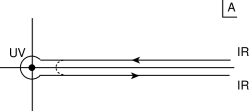
Figure 1: The solid line is the the Saalschutz contour in the complex area ($A$) plane, which is used to continue analytically the prefactor $\Gamma(-s)$ for $s\in Z^{+}$. It has been used in conventional quantum field theory to relate dimensional regularization to the Bogoliubov-Parasiuk-Hepp-Zimmermann renormalization method. The dashed line denotes the regularized contour, which avoids the ultraviolet fixed point $A\rightarrow 0$, which is used in the closed time-like path formalism.

Constraining the world-sheet area $A$ at a fixed value [3], one can use the following integral representation for $\Gamma(-s)$:

$$\Gamma(-s)=\int dAe^{-A}A^{-s-1},$$ (30)

where $A$ is the covariant area of the world-sheet. In the case $s=n^{+}\in{Z}^{+}$ one can then regularize by analytic continuation, replacing (30) by an integral along the Saalschutz contour shown in Fig. 1 [12, 9]. This is a well-known method of regularization in conventional field theory, where integrals of forms similar to (30) appear in terms of Feynman parameters.

A similar regularization was used to prove the equivalence of the Bogolubov-Parasiuk-Hepp-Zimmerman renormalization prescription with dimensional regularization in ordinary gauge field theories [13]. One result of such an analytic continuation is the appearance of imaginary parts in the respective correlation functions, which in our case are interpreted [12, 9] as renormalization-group instabilities of the system.

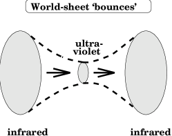
Figure 2: Schematic repesentation of the evolution of the world-sheet area as the renormalization-group scale moves along the contour of Fig. 1.

Interpreting the latter as an actual time flow, with the identification of the (world-sheet) zero mode with the target time [9], we then interpret the contour of Fig. 1 as implying evolution of the world-sheet area in both (negative and positive) directions of time as seen in Fig. 2, i.e., infrared fixed point $\to$ ultraviolet fixed point $\to$ infrared fixed point. In each half of the world-sheet diagram of fig. 2, the Zamolodchikov $C$ theorem [15] tells us that we have an irreversible Markov process.

This in turn implies a ‘bounce’ interpretation of the renormalization-group flow of Fig. 2, in which the infrared fixed point with large world-sheet area $A\to\infty$ is a ‘bounce’ point, similar to the corresponding picture in point-like field theory [14]. Therefore, the physical flow of time $t$ is taken to be opposite to the conventional renormalization-group flow, i.e., from the infrared to the ultraviolet ($A\to 0$) fixed point on the world sheet. In terms of the world-sheet zero mode of the Liouville field $\hat{\phi}_{0}$, we have $\hat{\phi}_{0}\sim{\rm ln}A\in\left(0,~{}-\infty\right)$. Our analysis in the previous Section shows that the effective potential term (27) vanishes in the limit $Q^{2}\to 0$, so this limit corresponds to a stable target-space theory. We stress once more that this is consistent with the disappearance (as $|Q^{2}|\to 0^{+}$) of tachyonic instabilities in the target-space theory, as manifested through tachyonic mass shifts $\Delta m^{2}=-|Q^{2}|<0$ of initially (i.e, before Liouville dressing) massless target-space excitations. Thus, the analysis of this paper reinforces the previous arguments that the (zero mode of the) world-sheet Liouville mode may be identified (up to a sign) with the target time.

6 Summary and Perspectives

We have demonstrated in this paper how a novel renormalization-group technique for controlling quantum effects by relaxing a mass parameter can be used to obtain non-perturbative results for non-critical string models. We have studied the behaviour of Liouville string theory as a function of the departure from criticality, as parametrized by the central-charge deficit $Q$. We have identified a renormalization-group fixed point in the limit $Q^{2}\to 0^{+}$, in which the dynamics of the Liouville field becomes trivial, as it neither propagates nor interacts, and the target space-time is of Minkowski type (in the supercritical string case). We have shown that the resulting theory is free of tachyonic instabilities in target space in the limit $|Q^{2}|\to 0^{+}$. This analysis supports the previous identification [9] of the (zero mode of the) Liouville mode with the target time.

This approach may in the future be used to discuss the transitions between linear-dilaton cosmological models with different values of $Q$, and ultimately the transition to an asymptotic state. It has been shown previously that $Q$ corresponds to the vacuum energy in conventional field-theoretical models of cosmological inflation [4, 9]. The transition from scalar field energy to relativistic particles has bee studied extensively within that framework, and our approach provides a framework for addressing such cosmological phase transitions in string theory.

Another area where this technique may be applied is the Quantum Hall effect (QHE). The different values of $Q$ correspond to different Hall conductivity plateaux, and our approach can be used to discuss transitions between these plateaux. The analogy between string cosmology and black-hole physics, on the one hand, and the QHE, on the other hand, has been advertised previously [5]. The novel renormalization-group described here provides a tool that can be used to quantify this relationship.

Appendix

We review here the construction of the effective action $\Gamma$ and derive the equation describing its evolution with $Q$. For reasons explained in the text, we restrict ourselves to the subcritical string case $Q^{2}\propto c^{*}-C>0$. The supercritical string case $Q^{2}<0$ is treated formally by means of analytic continuation. In terms of the microscopic field $\tilde{\phi}$, the bare action is

$$S=\int d^{2}\xi\left\{\frac{Q^{2}}{2}\partial_{a}\tilde{\phi}\partial^{a}\tilde{\phi}+\beta_{Q}R^{(2)}\tilde{\phi}+\mu^{2}P_{B}(\phi)e^{\tilde{\phi}}\right\},$$ (31)

The partition function, namely the functional of the source $j$, is defined as

$${\cal Z}[j]=\int{\cal D}[\tilde{\phi}]\exp\left(-S-\int d^{2}\xi~{}j\tilde{\phi}\right),$$ (32)

and is related to the functional $W$ that generates connected graphs by

$$W[j]=-\ln{\cal Z}[j].$$ (33)

The classical field $\phi$ is defined by differentiation of $W$ with respect to the source $j$, and we have

$$\frac{\delta W}{\delta j_{\xi}} = -\frac{1}{{\cal Z}}\frac{\partial{\cal Z}}{\partial j_{\xi}}=\frac{<\tilde{\phi}_{\xi}>}{{\cal Z}}=\phi_{\xi}$$

$$\frac{\delta^{2}W}{\delta j_{\xi}\delta j_{\zeta}} = \phi_{\xi}\phi_{\zeta}-\frac{<\tilde{\phi}_{\xi}\tilde{\phi}_{\zeta}>}{{\cal Z}},$$ (34)

where the quantum vacuum expectation value is

$$<\cdot\cdot\cdot>=\int{\cal D}[\tilde{\phi}](\cdot\cdot\cdot)\exp\left(-S-\int d^{2}\xi~{}j\tilde{\phi}\right).$$ (35)

The effective action $\Gamma$, a functional of the classical field $\phi$, is introduced as the Legendre transform of $W$:

$$\Gamma[\phi]=W[j]-\int j\phi,$$ (36)

where the source $j$ has to be seen as a functional of $\phi$. The functional derivatives of $\Gamma$ are then

$$\frac{\delta\Gamma}{\delta\phi_{\xi}} = -j_{\xi}$$

$$\frac{\delta^{2}\Gamma}{\delta\phi_{\xi}\delta\phi_{\zeta}} = -\left(\frac{\delta\phi_{\xi}}{\delta j_{\zeta}}\right)^{-1}=-\left(\frac{\delta^{2}W}{\delta j_{\xi}\delta j_{\zeta}}\right)^{-1}.$$ (37)

From eqs.(Appendix), the equation describing the evolution of $W$ with $Q^{2}$ is

$$\dot{W} = \frac{1}{{\cal Z}}\int d^{2}\xi\int d^{2}\zeta\left\{\frac{1}{2}\frac{\partial}{\partial\xi^{a}}\frac{\partial}{\partial\zeta_{a}}\left<\tilde{\phi}_{\xi}\tilde{\phi}_{\zeta}\right>+\dot{\beta}_{Q}R^{(2)}\left<\tilde{\phi}_{\xi}\right>\right\}\delta^{(2)}(\xi-\zeta)$$ (38)

$$= \int d^{2}\xi\left\{\frac{1}{2}\partial_{a}\phi\partial^{a}\phi+\dot{\beta}_{Q}R^{(2)}\phi\right\}-\frac{1}{2}\mbox{Tr}\left\{\frac{\partial}{\partial\xi_{a}}\frac{\partial}{\partial\zeta^{a}}\left(\frac{\delta^{2}W}{\delta j_{\xi}\delta j_{\zeta}}\right)\right\}.$$

In order to find the evolution equation for $\Gamma$, one should remember that its independent variables are $Q$ ad $\phi$, so that

$$\dot{\Gamma}=\dot{W}+\int d^{2}\xi~{}\frac{\delta W}{\delta j}\partial_{Q}j-\int d^{2}\xi~{}\partial_{Q}j\phi=\dot{W}.$$ (39)

Using the previous results, finally we have

$$\dot{\Gamma}=\int d^{2}\xi\left\{\frac{1}{2}\partial_{a}\phi\partial^{a}\phi+\dot{\beta}_{Q}R^{(2)}\phi\right\}+\frac{1}{2}\mbox{Tr}\left\{\frac{\partial}{\partial\xi_{a}}\frac{\partial}{\partial\zeta^{a}}\left(\frac{\delta^{2}\Gamma}{\delta\phi_{\xi}\delta\phi_{\zeta}}\right)^{-1}\right\}.$$ (40)

In order to extract physical quantities from the evolution equation (40), we assume the following functional dependence of the effective action:

$$\Gamma=\int d^{2}\xi\left\{\frac{Z_{Q}}{2}\partial_{a}\phi\partial^{a}\phi+\beta_{Q}R^{(2)}\phi+\mu^{2}P_{Q}(\phi)e^{\phi}\right\}.$$ (41)

We have then

$$\frac{\delta^{2}\Gamma}{\delta\phi_{\xi}\delta\phi_{\zeta}} = \left\{Z_{Q}\partial_{a}\partial^{a}+U^{{}^{\prime\prime}}_{Q}(\phi)\right\}\delta^{(2)}(\xi-\zeta),$$

$$\mbox{where}~{}~{}~{}U_{Q}(\phi)=\mu^{2}P_{Q}(\phi)e^{\phi},$$

and a prime denotes a derivative with respect to $\phi$. For the evolution of $P$ only, it would be enough to insert in the evolution equation (40) a constant field $\phi_{0}$. But in order to derive the evolution of $Z_{Q}$, one needs a varying field and we consider thus $\phi=\phi_{0}+2\rho\cos(k\xi)$, where $k$ is some fixed momentum. If ${\cal A}$ denotes the surface area of the world sheet, the effective action then reads

$$\Gamma={\cal A}\left(Z\rho^{2}k^{2}+\beta_{Q}R^{(2)}\phi_{0}+U_{Q}(\phi_{0})+\frac{1}{2}\rho^{2}U^{{}^{\prime\prime}}_{Q}(\phi_{0})+{\cal O}(\rho^{3})\right),$$ (43)

so that the evolution equation for $U$ is obtained by identifying the $k$-independent terms in eq.(40), and the evolution equation for $Z$ by identifying the terms proportional to $\rho^{2}k^{2}$.

The second derivative of the effective action reads for this configuration $\phi$, in Fourier components,

$$\frac{\delta^{2}\Gamma}{\delta\phi_{p}\delta\phi_{q}} = \left(Z_{Q}p^{2}+U_{Q}^{{}^{\prime\prime}}(\phi_{0})\right)(2\pi)^{2}\delta^{(2)}(p+q)$$

$$+\rho^{2}U^{{}^{\prime\prime\prime}}_{Q}(\phi_{0})(2\pi)^{2}\left[\delta^{(2)}(p+q+k)+\delta^{(2)}(p+q-k)\right]+{\cal O}(\rho^{3}).$$

The inverse of this matrix with components $p,q$ is computed using the following expansion

$$(A+B)^{-1}=A^{-1}-A^{-1}BA^{-1}+A^{-1}BA^{-1}BA^{-1}+\cdot\cdot\cdot,$$ (45)

where $A$ is a diagonal matrix with indices $p,q$, and $B$ is off-diagonal and proportional to $\rho^{2}$. In the previous expansion, the term linear in $A^{-1}$ is independent of $\rho,k$. It leads to the evolution of $U$, and makes the following contribution to the trace which appears in eq.(40):

$${\cal A}\int\frac{d^{2}p}{(2\pi)^{2}}\frac{p^{2}}{Z_{Q}p^{2}+U^{{}^{\prime\prime}}_{Q}(\phi_{0})}$$ (46)

$$= {\cal A}\frac{\Lambda^{2}}{4\pi Z_{Q}}-{\cal A}\frac{U^{{}^{\prime\prime}}_{Q}(\phi_{0})}{4\pi Z^{2}}\ln\left(1+\frac{Z_{Q}\Lambda^{2}}{U^{{}^{\prime\prime}}_{Q}(\phi_{0})}\right).$$

We note that the quadratic divergence is field-independent, and therefore is irrelevant. Also, the term linear in $B$, which appears in the expansion (45), has a vanishing trace since it is off-diagonal. The term quadratic in $B$ in the expansion (45) contains a contribution that is proportional to $\rho^{2}$ and independent of $k$, which does not bring any new information, since it corresponds to the evolution of $U^{{}^{\prime\prime}}$, as can be seen from eq.(43). It also contains a contribution proportional to $\rho^{2}k^{2}$, which leads to the evolution of $Z$. The corresponding trace is

$${\cal A}\rho^{2}\left[U^{{}^{\prime\prime\prime}}_{Q}(\phi_{0})\right]^{2}\int\frac{d^{2}p}{(2\pi)^{2}}\frac{4p^{2}}{\left(Z_{Q}p^{2}+U_{Q}^{{}^{\prime\prime}}(\phi_{0})\right)^{4}}\left(-Z_{Q}k^{2}+\frac{4Z_{Q}^{2}(kp)^{2}}{Z_{Q}p^{2}+U^{{}^{\prime\prime}}_{Q}(\phi_{0})}\right)+{\cal O}(k^{4})$$ (47)

$$= {\cal A}\frac{\rho^{2}k^{2}}{\pi Z_{Q}}\left[U^{{}^{\prime\prime\prime}}_{Q}(\phi_{0})\right]^{2}\int_{0}^{\infty}dx\left(\frac{-x}{\left(x+U_{Q}^{{}^{\prime\prime}}(\phi_{0})\right)^{4}}+\frac{2x^{2}}{\left(x+U_{Q}^{{}^{\prime\prime}}(\phi_{0})\right)^{5}}\right)+{\cal O}(k^{4})$$

$$= {\cal O}(k^{4}),$$

where we used the fact that, for any function $f(p^{2})$,

$$\int\frac{d^{2}p}{(2\pi)^{2}}(kp)^{2}f(p^{2})=\frac{k^{2}}{8\pi}\int d(p^{2})p^{2}f(p^{2}).$$ (48)

As a consequence, $Z$ does not receive quantum corrections. Finally, the evolution equation for $P$ is found from eqs.(40), (43) and (46) where we disregard the field-independent quadratic divergence, to be

$$\dot{P}_{Q}(\phi)=-\frac{P_{Q}(\phi)+2P_{Q}^{{}^{\prime}}(\phi)+P_{Q}^{{}^{\prime\prime}}(\phi)}{8\pi Z_{Q}^{2}}\ln\left(1+\frac{Z_{Q}e^{-\phi}\Lambda^{2}/\mu^{2}}{P_{Q}(\phi)+2P_{Q}^{{}^{\prime}}(\phi)+P_{Q}^{{}^{\prime\prime}}(\phi)}\right).$$ (49)

The reader can now see easily why the supercritical string case $Q^{2}<0$ presents certain problems that can be treated by analytic continuation.

Considering the case $Q^{2}<0$ and a Euclidean world sheet metric, we have

$$\frac{\delta^{2}S(\phi_{0})}{\delta\phi(p)\delta\phi(q)}=\left\{-|Q^{2}|(p_{1}^{2}+p_{2}^{2})+\mu^{2}e^{\phi_{0}}\right\}\delta^{(2)}(p+q).$$ (50)

The propagator is the inverse of this, and hence cannot be integrated because of the pole, whose presence is linked to the supercriticality of the string. This pole is not the usual one corresponding to a mass. Indeed, if one returns to a Minkowski world-sheet metric, one obtains:

$$\frac{\delta^{2}S(\phi_{0})}{\delta\phi(p)\delta\phi(q)}=\left\{|Q^{2}|(p_{0}^{2}-p_{1}^{2})+\mu^{2}e^{\phi_{0}}\right\}\delta^{(2)}(p+q),$$ (51)

where $p_{0}=ip_{2}$. One should perform another ‘Wick rotation’ on $p_{1}$ in order to treat the problem properly.

Formally, these issues are resolved simply by treating the $Q^{2}<0$ case in our method by the above-mentioned complex continuation of both $Q\to iQ$ and the Liouville scaling exponents: $\alpha=\frac{(1+\varepsilon_{Q})}{Q}\to i\alpha$.

References

- [1] I. Antoniadis, C. Bachas, J. R. Ellis and D. V. Nanopoulos, Phys. Lett. B 211, 393 (1988); Nucl. Phys. B 328, 117 (1989); Phys. Lett. B 257, 278 (1991).
- [2] J. R. Ellis, N. E. Mavromatos, D. V. Nanopoulos and A. Sakharov, New J. Phys. 6, 171 (2004) [arXiv:gr-qc/0407089]; J. R. Ellis, N. E. Mavromatos, D. V. Nanopoulos and M. Westmuckett, Int. J. Mod. Phys. A 21, 1379 (2006) [arXiv:gr-qc/0508105], and references therein.
- [3] F. David, Mod. Phys. Lett. A 3, 1651 (1988); J. Distler and H. Kawai, “Conformal Field Theory And 2-D Quantum Gravity Or Who’s Afraid Of Joseph Nucl. Phys. B 321, 509 (1989).
- [4] J. R. Ellis, N. E. Mavromatos and D. V. Nanopoulos, Mod. Phys. Lett. A 10, 1685 (1995) [arXiv:hep-th/9503162]; G. A. Diamandis, B. C. Georgalas, N. E. Mavromatos, E. Papantonopoulos and I. Pappa, Int. J. Mod. Phys. A 17, 2241 (2002) [arXiv:hep-th/0107124].
- [5] J. R. Ellis, N. E. Mavromatos and D. V. Nanopoulos, Phys. Lett. B 296, 40 (1992) [arXiv:hep-th/9209013].
- [6] J. Alexandre and J. Polonyi, Annals Phys. 288, 37 (2001) [arXiv:hep-th/0010128].
- [7] J. Alexandre, J. Ellis and N. E. Mavromatos, arXiv:hep-th/0610072.
- [8] E. D’Hoker and R. Jackiw, Phys. Rev. D 26, 3517 (1982).
- [9] J. R. Ellis, N. E. Mavromatos and D. V. Nanopoulos, arXiv:hep-th/9403133, Published in Erice Subnuclear Series, 1993: pp 1-66; arXiv:hep-th/9805120.
- [10] E. Gravanis and N. E. Mavromatos, Phys. Lett. B 547, 117 (2002) [arXiv:hep-th/0205298].
- [11] M. Goulian and M. Li, Phys. Rev. Lett. 66, 2051 (1991).
- [12] I. Kogan, Phys. Lett. B265, 269 (1991).
- [13] T. Roy and A. Roy Chowdhuri, Phys. Rev. D15 3768 (1977).
- [14] S. Coleman, Phys. Rev. D15 2929 (1977); 1248 (E) (1977). C. Callan and S. Coleman, Phys. Rev. D16, 1762 (1977).
- [15] A.B. Zamolodchikov, JETP Lett. 43, 730 (1986); Sov. J. Nucl. Phys. 46, 1090 (1987).