UMTG–251

Finite size effects in the spin-1 XXZ
and supersymmetric sine-Gordon models
with Dirichlet boundary conditions
Changrim Ahn ^,2, Rafael I. Nepomechie and Junji Suzuki

Starting from the Bethe Ansatz solution of the open integrable spin-1 XXZ quantum spin chain with diagonal boundary terms, we derive a set of nonlinear integral equations (NLIEs), which we propose to describe the boundary supersymmetric sine-Gordon model BSSG⁺ with Dirichlet boundary conditions on a finite interval. We compute the corresponding boundary $S$ matrix, and find that it coincides with the one proposed by Bajnok, Palla and Takács for the Dirichlet BSSG⁺ model. We derive a relation between the (UV) parameters in the boundary conditions and the (IR) parameters in the boundary $S$ matrix. By computing the boundary vacuum energy, we determine a previously unknown parameter in the scattering theory. We solve the NLIEs numerically for intermediate values of the interval length, and find agreement with our analytical result for the effective central charge in the UV limit and with boundary conformal perturbation theory.

1 Introduction

Much can be learned from studying quantum field theories in finite volume. This is particularly true for $1+1$-dimensional integrable QFTs, for which there are effective descriptions in both the infrared (infinite size) and ultraviolet (zero size) limits, namely, massive factorized scattering theory [1, 2, 3] and conformal field theory (CFT) [4, 5], respectively. Moreover, at least for some examples, there also exist effective descriptions in terms of certain nonlinear integral equations (NLIEs) for general system size.

A case in point is the sine-Gordon (SG) model on a circle (periodic boundary conditions) [6]-[8], and on an interval with either Dirichlet [9, 10] or general integrable [11] boundary conditions. NLIEs have been obtained in these papers from Bethe Ansatz solutions of corresponding critical spin-$\frac{1}{2}$ XXZ chains [12]-[15], with a mass scale introduced by means of an alternating inhomogeneity parameter ($\pm\Lambda$). Among the quantities that have been computed from these NLIEs are bulk and boundary $S$ matrices (IR limit), bulk and boundary energies, and central charge and conformal dimensions (UV limit). Moreover, Casimir energies in the near UV region obtained by numerically solving the NLIEs agree well with those obtained using the truncated conformal space approach (TCSA) [16, 17] and conformal perturbation theory.

In the NLIE approach one generally deals with three sets of parameters: the UV parameters appearing in the action, the IR parameters appearing in the $S$ matrices, and the lattice parameters in terms of which the NLIE is initially formulated. (See Figure 1.) In principle, by matching the UV and IR limits of the NLIE with corresponding known results, one can deduce the “lattice $\leftrightarrow$ UV” and “lattice $\leftrightarrow$ IR” relations, respectively. If the “UV $\leftrightarrow$ IR” relation is also known, then the consistency of these three sets of relations can be checked. For the sine-Gordon model, for which the “UV $\leftrightarrow$ IR” relation for the boundary parameters has been determined [18], this consistency has been established for both the bulk and boundary parameters.

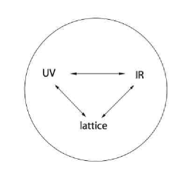
Figure 1: Three sets of parameters and their relations

Much less is known about the supersymmetric sine-Gordon (SSG) model [19]-[22],

$${\cal L}={1\over 2}\partial_{\mu}\varphi\,\partial^{\mu}\varphi+{1\over 2}i\bar{\Psi}\gamma^{\mu}\partial_{\mu}\Psi-{m_{0}\over 2}\cos(\beta\varphi)\bar{\Psi}\Psi+{m_{0}^{2}\over 2\beta^{2}}\cos^{2}(\beta\varphi)\,,$$ (1.1)

where $\varphi$ is a real scalar field, $\Psi$ is a Majorana Fermion field, $m_{0}$ is a mass parameter, and $\beta\in\left(0\,,4\pi\right)$ is a dimensionless coupling constant. Indeed, for the case of periodic boundary conditions, an NLIE was proposed only recently [23], and derived in [24, 25] from the Bethe Ansatz solution of the integrable spin-1 XXZ chain [26, 27]. While the ground state of the critical spin-$\frac{1}{2}$ chain is described by a sea of real Bethe roots, the ground state of the critical spin-1 chain is described by a sea of approximate “two-strings”, i.e., certain complex conjugate pairs of Bethe roots. As a result, the familiar method [7] of deriving the NLIE, based on the Bethe Ansatz equations and the corresponding counting function, does not seem to work for the spin-1 case. Nevertheless, an NLIE can be derived [24, 25] from the model’s $T-Q$ equations, in a manner similar to the original approach [6]. Very recently, the periodic spin-1 XXZ/SSG NLIE for excited states was shown [28] to have the correct UV and IR limits. In particular, the bulk soliton $S$ matrix [22] was obtained from the IR limit of the NLIE.

Our goal has been to find an NLIE for the boundary supersymmetric sine-Gordon model on an interval with general integrable boundary conditions [29]-[32]. This field theory is of interest as a toy model with boundary that is both integrable and supersymmetric; and it may also have applications to superstring theory [33]. Since a Bethe Ansatz solution of the corresponding open spin-1 XXZ chain with general integrable boundary terms [34] is still not known, we focus here on the special case of diagonal boundary terms, whose solution is already available [35]. The homogeneous chain has the local Hamiltonian

$$H=\sum_{n=1}^{N-1}H_{n,n+1}+\ b.t.\,,$$ (1.2)

where the bulk terms $H_{n,n+1}$ are those of the Fateev-Zamolodchikov [26] spin chain,

$$H_{n,n+1} = \sigma_{n}-(\sigma_{n})^{2}-2\sin^{2}\gamma\left[\sigma_{n}^{z}+(S^{z}_{n})^{2}+(S^{z}_{n+1})^{2}-(\sigma_{n}^{z})^{2}\right]$$ (1.3)

$$+ 4\sin^{2}(\frac{\gamma}{2})\left(\sigma_{n}^{\bot}\sigma_{n}^{z}+\sigma_{n}^{z}\sigma_{n}^{\bot}\right)\,,$$

where

$$\sigma_{n}=\vec{S}_{n}\cdot\vec{S}_{n+1}\,,\quad\sigma_{n}^{\bot}=S^{x}_{n}S^{x}_{n+1}+S^{y}_{n}S^{y}_{n+1}\,,\quad\sigma_{n}^{z}=S^{z}_{n}S^{z}_{n+1}\,,$$ (1.4)

and $\vec{S}_{n}$ are spin-1 generators of $SU(2)$; and the diagonal boundary terms are give by

$$b.t. = \frac{1}{2}\sin(2\gamma)\Big{\{}-\left[\cot\eta_{-}+\cot(\eta_{-}-\gamma)\right]S^{z}_{1}+\left[\cot\eta_{-}-\cot(\eta_{-}-\gamma)\right](S^{z}_{1})^{2}$$ (1.5)

$$- \left[\cot\eta_{+}+\cot(\eta_{+}-\gamma)\right]S^{z}_{N}+\left[\cot\eta_{+}-\cot(\eta_{+}-\gamma)\right](S^{z}_{N})^{2}\Big{\}}\,.$$

The bulk and boundary parameters are $\gamma$ and $\eta_{\pm}$, respectively.

We propose that, in analogy with the spin-$\frac{1}{2}$ XXZ/SG model, this open spin chain corresponds to the boundary SSG model on an interval $\left[x_{-}\,,x_{+}\right]$ with Dirichlet boundary conditions,

$$\varphi(x_{-},t)=\varphi_{-}\,,\quad\varphi(x_{+},t)=\varphi_{+}\,,\quad\psi(x_{-},t)-\bar{\psi}(x_{-},t)=0\,,\quad\psi(x_{+},t)-\bar{\psi}(x_{+},t)=0\,,$$ (1.6)

where $\psi$ and $\bar{\psi}$ are the spinor components of the Majorana field $\Psi$. These boundary conditions follow from the boundary action [30] in the limit that the boundary mass parameters tend to infinity. That the diagonal boundary terms (1.5) of the spin-1 XXZ chain correspond to the Dirichlet boundary conditions (1.6) of the SSG model is consistent with the fact that $S^{z}$ and topological charge are conserved in the two models, respectively, and also that both models are integrable.

There are actually two known sets of integrable supersymmetric boundary conditions for the boundary SSG model [30]. Following [32], we shall refer to the set (1.6) as Dirichlet BSSG⁺, and to the set with $\psi+\bar{\psi}=0$ at both ends as Dirichlet BSSG^-.

We derive an NLIE for the Dirichlet BSSG⁺ model, circumventing (as in [25]) the difficulties posed by the ground-state sea of two-strings by identifying suitable auxiliary functions from the model’s $T-Q$ equations [35], and exploiting their analytic properties. By analyzing the IR limit of this NLIE, we compute the soliton boundary $S$ matrix, which coincides with the one proposed for the Dirichlet BSSG⁺ model by Bajnok et al. [32]. We propose the “UV $\leftrightarrow$ IR” relation for the boundary parameters, for the special case of Dirichlet boundary conditions, on the basis of our NLIE and its UV and IR limits. By computing the boundary vacuum energy, we determine a previously unknown parameter in the scattering theory [32]. We solve the NLIEs numerically for intermediate values of the volume, and find agreement with our analytical result for the effective central charge in the UV limit and with boundary conformal perturbation theory, and confirm the UV-IR relation.

The outline of this paper is as follows. In Section 2 we rederive the NLIE for the spin-$\frac{1}{2}$ XXZ/sine-Gordon model with Dirichlet boundary conditions [9]. However, we use the method which we apply to the spin-1 case (which differs from the approach used in [9]), and therefore, this serves as a valuable warm-up exercise for the latter problem. In Section 3 we turn to our main interest, the spin-1 XXZ/supersymmetric sine-Gordon model with Dirichlet boundary conditions. We sketch the derivation of the NLIE, relegating some of the details to Appendix B. In particular, we determine the boundary terms $\mathsf{P}_{bdry}(\theta)$ and $\mathsf{P}_{y}(\theta)$ which encode boundary effects. Section 4 is devoted to an analysis of the IR limit of this NLIE. In the course of computing the corresponding boundary $S$ matrix, we determine the “lattice $\leftrightarrow$ IR” relation for the boundary parameters. In Section 5, we analyze the UV limit of our NLIE, and compare with the expected CFT result. In this way, we obtain a boundary “UV $\leftrightarrow$ lattice” relation, and therefore finally the “UV $\leftrightarrow$ IR” relation for the boundary parameters. In Section 6 we compute the effective central charge of the Dirichlet SSG model using first-order boundary conformal perturbation theory, and compare with numerical NLIE results. We conclude in Section 7 with a discussion of our results and with some comments on various open problems. Some important technical details are explained in the appendices.

2 Spin-$\frac{1}{2}$ XXZ/SG with Dirichlet boundary conditions

We rederive here the NLIE for the spin-$\frac{1}{2}$ XXZ/sine-Gordon model with Dirichlet boundary conditions [9]. However, in contrast to the familiar approach [7] used in [9], we do not introduce the counting function. Instead, we identify suitable auxiliary functions from the model’s $T-Q$ equation, and exploit their analyticity properties. We shall use the same method to treat the spin-1 XXZ/supersymmetric sine-Gordon model in Section 3.

2.1 $T-Q$ equation

The transfer-matrix eigenvalues $T(x)$ of the inhomogeneous open spin-$\frac{1}{2}$ XXZ chain with Dirichlet boundary conditions satisfy the $T-Q$ equation [14]

$$T(x)=T^{(+)}(x)+T^{(-)}(x)\,,\qquad T^{(\pm)}(x)\equiv\sinh(2x\pm i\gamma)\,B^{(\pm)}(x)\,\phi(x\pm\frac{i\gamma}{2})\frac{Q(x\mp i\gamma)}{Q(x)}\,,$$ (2.1)

where

$$\phi(x) = \sinh^{N}(x-\Lambda)\sinh^{N}(x+\Lambda)\,,$$

$$B^{(\pm)}(x) = \sinh(x\pm\frac{i\gamma H_{+}}{2})\sinh(x\pm\frac{i\gamma H_{-}}{2})\,,$$

$$Q(x) = \prod_{k=1}^{M}\sinh(x-v_{k})\sinh(x+v_{k})\,.$$ (2.2)

We denote the bulk parameter by $\gamma$ ($0<\gamma<\pi$), and the boundary parameters by $H_{\pm}$. Moreover, $\Lambda$ is the inhomogeneity parameter which provides a mass scale; $N$ is the number of spins; and the $M$ zeros $v_{k}$ of $Q(x)$ are the Bethe roots. Note that $T(-x)=-T(x)$.

For the homogeneous case $\Lambda=0$, a local Hamiltonian is obtained from the first derivative of the transfer matrix $T(x)$ [14]. However, for the inhomogeneous case $\Lambda\neq 0$ which we consider here, the definition of energy is less clear. We shall follow the prescription of Reshetikhin and Saleur [36], which implies

$$E=-\frac{g}{a}\left\{\frac{d}{dx}\ln T(x)\Bigg{|}_{x=\Lambda+\frac{i\gamma}{2}}-\frac{d}{dx}\ln T(x)\Bigg{|}_{x=\Lambda-\frac{i\gamma}{2}}\right\}\,,$$ (2.3)

where $a$ is the lattice spacing, and $g$ is given by

$$g=-\frac{i\gamma}{4\pi}\,.$$ (2.4)

One can verify that this definition has the correct $\Lambda\rightarrow 0$ limit.

2.2 Derivation of NLIE

We define the auxiliary functions $a(x)$ and $\bar{a}(x)$ by

$$a(x)={\sinh(2x+i\gamma)\,B^{(+)}(x)\,\phi(x+\frac{i\gamma}{2})\,Q(x-i\gamma)\over{\sinh(2x-i\gamma)\,B^{(-)}(x)\,\phi(x-\frac{i\gamma}{2})\,Q(x+i\gamma)}}\,,\qquad{\bar{a}}(x)=a(-x)={1\over a(x)}\,.$$ (2.5)

The transfer-matrix eigenvalues can then be written as

$$T(x) = \sinh(2x-i\gamma)\,B^{(-)}(x)\,\phi(x-\frac{i\gamma}{2}){Q(x+i\gamma)\over{Q(x)}}A(x)$$ (2.6)

$$= \sinh(2x+i\gamma)\,B^{(+)}(x)\,\phi(x+\frac{i\gamma}{2}){Q(x-i\gamma)\over{Q(x)}}{\bar{A}}(x)\,,$$

where

$$A(x)=1+a(x)\,,\quad{\bar{A}}(x)=1+{\bar{a}}(x)\,.$$ (2.7)

The Bethe Ansatz equations are given by

$$A(v_{k})=0\,,\qquad k=1\,,\ldots\,,M\,.$$ (2.8)

We consider the ground state. For simplicity, we restrict the boundary parameters $H_{\pm}$ to the interval

$$0<H_{\pm}<\frac{\pi}{\gamma}\,.$$ (2.9)

We argue in Appendix A.1 that the boundary parameters should be further restricted to the range

$$\frac{\pi}{\gamma}-2<H_{+}+H_{-}<\frac{3\pi}{\gamma}-2$$ (2.10)

in order for the ground state to have $M=N/2$ real Bethe roots $v_{k}$ and no holes, except for one hole at the origin. That is, $T(x)$ does not have zeros near the real axis except for a simple zero at the origin. To remove this root, we define

$$\check{T}(x)={T(x)\over\mu(x)}\,,$$ (2.11)

where $\mu(x)$ is any function whose only real root is a simple zero at the origin, in particular $\mu(0)=0\,,\ \mu^{\prime}(0)\neq 0$, so that $\check{T}(x)$ is analytic and nonzero (ANZ) when $x$ is near the real axis. (We use a prime $(\ ^{\prime}$) to denote differentiation with respect to $x$.) It is convenient to introduce the compact notation

$$\check{T}(x)=t_{-}(x)\,{Q(x+i\gamma)\over{Q(x)}}A(x)=t_{+}(x)\,{Q(x-i\gamma)\over{Q(x)}}\bar{A}(x)\,,$$ (2.12)

where

$$t_{\pm}(x)={\sinh(2x\pm i\gamma)\over\mu(x)}B^{(\pm)}(x)\,\phi(x\pm\frac{i\gamma}{2})\,.$$ (2.13)

Since $\ln\check{T}(x)$ is analytic near the real axis, Cauchy’s theorem gives

$$0=\oint_{C}dx\ [\ln\check{T}(x)]^{\prime\prime}e^{ikx}\,,$$ (2.14)

where we choose the contour $C$ as in Figure 2.

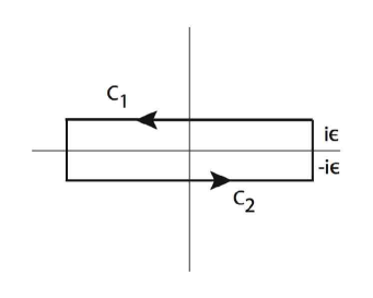
Figure 2: Integration contour

Dividing the contour $C=C_{1}+C_{2}$, where $C_{1}$ and $C_{2}$ have imaginary parts $\pm i\epsilon$ with $\epsilon$ small and positive respectively, this integral can be written as

$$0 = \int_{C_{1}}dx\ \left[\ln t_{+}(x)\right]^{\prime\prime}e^{ikx}+\int_{C_{1}}dx\ \left\{\ln\left[{Q(x-i\gamma)\over Q(x)}\right]\right\}^{\prime\prime}e^{ikx}+\int_{C_{1}}dx\ \left[\ln{\bar{A}}(x)\right]^{\prime\prime}e^{ikx}$$

$$+ \int_{C_{2}}dx\ \left[\ln t_{-}(x)\right]^{\prime\prime}e^{ikx}+\int_{C_{2}}dx\ \left\{\ln\left[{Q(x+i\gamma)\over Q(x)}\right]\right\}^{\prime\prime}e^{ikx}+\int_{C_{2}}dx\ \left[\ln A(x)\right]^{\prime\prime}e^{ikx}\,.$$

In terms of Fourier transforms defined along $C_{2}$ and $C_{1}$ by

$$\widehat{Lf^{\prime\prime}}(k)=\int_{C_{2}}dx\ [\ln f(x)]^{\prime\prime}e^{ikx}\,,\qquad\widehat{{\cal L}f^{\prime\prime}}(k)=\int_{C_{1}}dx\ [\ln f(x)]^{\prime\prime}e^{ikx}\,,$$ (2.15)

respectively, we can rewrite

$$\int_{C_{1}}dx\ \left\{\ln\left[{Q(x-i\gamma)\over Q(x)}\right]\right\}^{\prime\prime}e^{ikx} = -\widehat{LQ^{\prime\prime}}(k)\left(e^{-\gamma k}-e^{-\pi k}\right)\,,$$

$$\int_{C_{2}}dx\ \left\{\ln\left[{Q(x+i\gamma)\over Q(x)}\right]\right\}^{\prime\prime}e^{ikx} = \widehat{LQ^{\prime\prime}}(k)\left[e^{(\gamma-\pi)k}-1\right]\,,$$ (2.16)

where we have used the periodicity

$$Q(x)=Q(x-i\pi),\quad x\in C_{1},\qquad{\rm and}\qquad Q(x+i\gamma)=Q(x+i\gamma-i\pi),\quad x\in C_{2}\,.$$ (2.17)

Defining

$$C(k)\equiv\int_{C_{1}}dx\left[\ln t_{+}(x)\right]^{\prime\prime}e^{ikx}+\int_{C_{2}}dx\left[\ln t_{-}(x)\right]^{\prime\prime}e^{ikx}\,,$$ (2.18)

we obtain

$$\widehat{LQ^{\prime\prime}}(k)={e^{\frac{\pi k}{2}}\over 4\cosh(\frac{\gamma k}{2})\sinh\left((\pi-\gamma)\frac{k}{2}\right)}\left[\widehat{LA^{\prime\prime}}(k)+\widehat{{\cal L}{\bar{A}}^{\prime\prime}}(k)+C(k)\right]\,.$$ (2.19)

This is the main consequence of analyticity.

It follows from the definition of $a(x)$ (2.5) that

$$\widehat{La^{\prime\prime}}(k)=\int_{C_{2}}dx\ \left\{\ln\left[{Q(x-i\gamma)\over Q(x+i\gamma)}\right]\right\}^{\prime\prime}e^{ikx}+D(k)\,,$$ (2.20)

where $D(k)$ is defined by

$$D(k)=\int_{C_{2}}dx\ \left\{\ln\left[{\sinh(2x+i\gamma)\,B^{(+)}(x)\,\phi(x+\frac{i\gamma}{2})\over\sinh(2x-i\gamma)\,B^{(-)}(x)\,\phi(x-\frac{i\gamma}{2})}\right]\right\}^{\prime\prime}e^{ikx}\,.$$ (2.21)

Using again the periodicity of $Q(x)$, we obtain

$$\widehat{La^{\prime\prime}}(k)=\widehat{LQ^{\prime\prime}}(k)\left[e^{-\gamma k}-e^{(\gamma-\pi)k}\right]+D(k)\,.$$ (2.22)

Inserting (2.19) into (2.22) yields

$$\widehat{La^{\prime\prime}}(k)={\widehat{G}}(k)\left[\widehat{LA^{\prime\prime}}(k)+\widehat{{\cal L}{\bar{A}}^{\prime\prime}}(k)\right]+C_{T}(k)\,,$$ (2.23)

where

$${\widehat{G}}(k) = {\sinh\left((\pi-2\gamma)\frac{k}{2}\right)\over 2\cosh(\frac{\gamma k}{2})\sinh\left((\pi-\gamma)\frac{k}{2}\right)}\,,$$ (2.24)

$$C_{T}(k) = {\widehat{G}}(k)\,C(k)+D(k)\,.$$ (2.25)

The evaluation of $C_{T}(k)$ is tedious but straightforward. To this end, we make use of the identities

$$\int_{C_{2}}{dx\over 2\pi}\left[\ln\sinh(x-i\alpha)\right]^{\prime\prime}e^{ikx}=e^{-k(\alpha-n\pi)}\psi(k)\,,\qquad\psi(k)\equiv{k\over 1-e^{-\pi k}}\,,$$ (2.26)

where $n$ is an integer such that $0<\Re e(\alpha-n\pi)<\pi$, and

$$\int_{C_{2}}{dx\over 2\pi}\left[\ln\sinh(2x)\right]^{\prime\prime}e^{ikx}={k\over 1-e^{-\frac{\pi k}{2}}}\equiv\psi_{2}(k)\,.$$ (2.27)

The result is (B.6)

$$C_{T}(k) = -2\pi k\Bigg{\{}{N\cos(\Lambda k)\over\cosh({\gamma k\over 2})}+{\sinh\left((\gamma H_{+}-\pi)\frac{k}{2}\right)+\sinh\left((\gamma H_{-}-\pi)\frac{k}{2}\right)\over 2\cosh({\gamma k\over 2})\sinh\left((\gamma-\pi)\frac{k}{2}\right)}$$ (2.28)

$$+{\cosh({\gamma k\over 4})\sinh\left((2\gamma-\pi)\frac{k}{4}\right)\over\cosh({\gamma k\over 2})\sinh\left((\gamma-\pi)\frac{k}{4}\right)}\Bigg{\}}\,.$$

The result (2.23) is the NLIE for the lattice sine-Gordon model with Dirichlet boundary conditions in Fourier space. Passing to coordinate space, and integrating twice, we obtain

$$\ln a(x) = \int_{-\infty}^{\infty}dx^{\prime}\ G(x-x^{\prime}+i\epsilon)\ln A(x^{\prime}-i\epsilon)-\int_{-\infty}^{\infty}dx^{\prime}\ G(x-x^{\prime}-i\epsilon)\ln\bar{A}(x^{\prime}+i\epsilon)$$ (2.29)

$$- i2N\tan^{-1}\left({\sinh\frac{\pi x}{\gamma}\over\cosh\frac{\pi\Lambda}{\gamma}}\right)+i\,P_{bdry}(x)+i\pi\,,$$

where $G(x)$ is the Fourier transform of $\widehat{G}(k)$ (2.24)

$$G(x)={1\over 2\pi}\int_{-\infty}^{\infty}dk\ e^{-ikx}\ \widehat{G}(k)\,,$$ (2.30)

$P_{bdry}(x)$ is given by

$$P_{bdry}(x)=\int_{0}^{x}dx^{\prime}\,R(x^{\prime})=\frac{1}{2}\int_{-x}^{x}dx^{\prime}\,R(x^{\prime})\,,$$ (2.31)

and $R(x)$ is the Fourier transform of $\hat{R}(k)$,

$$\hat{R}(k) = -2\pi\Bigg{\{}{\sinh\left((\gamma H_{+}-\pi)\frac{k}{2}\right)+\sinh\left((\gamma H_{-}-\pi)\frac{k}{2}\right)\over 2\cosh({\gamma k\over 2})\sinh\left((\gamma-\pi)\frac{k}{2}\right)}$$ (2.32)

$$\quad+{\cosh({\gamma k\over 4})\sinh\left((2\gamma-\pi)\frac{k}{4}\right)\over\cosh({\gamma k\over 2})\sinh\left((\gamma-\pi)\frac{k}{4}\right)}\Bigg{\}}\,.$$

The integration constant is explained in Section C.1.

The continuum limit consists of taking $\Lambda\rightarrow\infty$ (leading to a simplification in the driving term, $-i2N\tan^{-1}\left({\sinh\frac{\pi x}{\gamma}\over\cosh\frac{\pi\Lambda}{\gamma}}\right)\sim-i4Ne^{-\frac{\pi\Lambda}{\gamma}}\sinh\frac{\pi x}{\gamma}$), together with $N\rightarrow\infty$ and lattice spacing $a\rightarrow 0$, such that the interval length $L\equiv x_{+}-x_{-}$ and the soliton mass $m$ are given by

$$L=Na\,,\qquad m={2\over a}e^{-\frac{\pi\Lambda}{\gamma}}\,.$$ (2.33)

The driving term therefore becomes $-i2mL\sinh\theta$, where the renormalized rapidity $\theta$ is defined as

$$\theta=\frac{\pi x}{\gamma}\,.$$ (2.34)

The resulting NLIE

$$\ln\mathsf{a}(\theta) = \int_{-\infty}^{\infty}d\theta^{\prime}\ \mathsf{G}(\theta-\theta^{\prime}+i\varepsilon)\ln\mathsf{A}(\theta^{\prime}-i\varepsilon)-\int_{-\infty}^{\infty}d\theta^{\prime}\ \mathsf{G}(\theta-\theta^{\prime}-i\varepsilon)\ln\bar{}\mathsf{A}(\theta^{\prime}+i\varepsilon)$$ (2.35)

$$- i2mL\sinh\theta+i\,\mathsf{P}_{bdry}(\theta)+i\pi\,,$$

where we have defined

$$\varepsilon=\frac{\pi\epsilon}{\gamma}\,,\quad\!\mathsf{a}(\theta)=a(\frac{\gamma\theta}{\pi})\,,\quad\!\mathsf{A}(\theta)=A(\frac{\gamma\theta}{\pi})\,,\quad\!\mathsf{P}_{bdry}(\theta)=P_{bdry}(\frac{\gamma\theta}{\pi})\,,\quad\!\mathsf{G}(\theta)=\frac{\gamma}{\pi}G(\frac{\gamma\theta}{\pi})\,,$$ (2.36)

agrees with [9].

2.3 Vacuum and Casimir energies

Since our approach avoids introducing the counting function and the density of Bethe roots, the energy computation also differs from that of the conventional approach [7]. The main idea is to express the energy in terms of $\widehat{LQ}(k)$, and then make use of the consequence (2.19) of analyticity.

The energy is given by (2.3). From the $T-Q$ equation (2.1) and the fact $\phi(\Lambda)=0$, we see that

$$\frac{d}{dx}\ln T(x)\Bigg{|}_{x=\Lambda\pm\frac{i\gamma}{2}}=\frac{d}{dx}\ln T^{(\pm)}(x)\Bigg{|}_{x=\Lambda\pm\frac{i\gamma}{2}}\,.$$ (2.37)

Hence, the energy (2.3) can be written as

$$E = -\frac{g}{a}\frac{d}{dx}\left\{\ln T^{(+)}(x+\frac{i\gamma}{2})-\ln T^{(-)}(x-\frac{i\gamma}{2})\right\}\bigg{|}_{x=\Lambda}$$ (2.38)

$$= -\frac{g}{a}\int\frac{dk}{2\pi}e^{-ik\Lambda}\left[e^{\frac{\gamma k}{2}}\widehat{LT^{(+)^{\prime}}}(k)-e^{-\frac{\gamma k}{2}}\widehat{LT^{(-)^{\prime}}}(k)\right]\,,$$

where we used the fact (see (2.15))

$$[\ln f(x)]^{\prime}=\int\frac{dk}{2\pi}\ \widehat{Lf^{\prime}}(k)\ e^{-ikx}\,,\qquad x\in C_{2}\,.$$ (2.39)

Since

$$T^{(\pm)}(x\pm\frac{i\gamma}{2})=\sinh(2x\pm 2i\gamma)\,B^{(\pm)}\left(x\pm\frac{i\gamma}{2}\right)\phi(x\pm i\gamma){Q\left(x\mp\frac{i\gamma}{2}\right)\over{Q\left(x\pm\frac{i\gamma}{2}\right)}},$$ (2.40)

we can compute the Fourier transforms $e^{\pm\frac{\gamma k}{2}}\widehat{LT^{(\pm)^{\prime}}}(k)$,

$$e^{-\frac{\gamma k}{2}}\widehat{LT^{(-)^{\prime}}}(k) = e^{-{\gamma k\over{2}}}\widehat{LB^{(-)^{\prime}}}(k)+e^{-\gamma k}\widehat{L\phi^{\prime}}(k)+e^{-\gamma k}\frac{2\pi\psi_{2}(k)}{(-ik)}$$

$$- 2e^{-\frac{\pi k}{2}}\sinh((\pi-\gamma)\frac{k}{2})\widehat{LQ^{\prime}}(k)\,,$$

$$e^{\frac{\gamma k}{2}}\widehat{LT^{(+)^{\prime}}}(k) = e^{{\gamma k\over{2}}}\widehat{LB^{(+)^{\prime}}}(k)+e^{(\gamma-\pi)k}\widehat{L\phi^{\prime}}(k)+e^{(\gamma-\frac{\pi}{2})k}\frac{2\pi\psi_{2}(k)}{(-ik)}$$ (2.41)

$$+ 2e^{-\frac{\pi k}{2}}\sinh((\pi-\gamma)\frac{k}{2})\widehat{LQ^{\prime}}(k)\,.$$

We can eliminate $\widehat{LQ^{\prime}}(k)$ using (2.19) and the fact $\widehat{Lf^{\prime}}(k)={1\over(-ik)}\widehat{Lf^{\prime\prime}}(k)$,

$$\widehat{LQ^{\prime}}(k) = {1\over(-ik)}{e^{\frac{\pi k}{2}}\over 4\cosh(\frac{\gamma k}{2})\sinh\left((\pi-\gamma)\frac{k}{2}\right)}\left[\widehat{LA^{\prime\prime}}(k)+\widehat{{\cal L}{\bar{A}}^{\prime\prime}}(k)+C(k)\right]$$ (2.42)

$$= {e^{\frac{\pi k}{2}}\over 4\cosh(\frac{\gamma k}{2})\sinh\left((\pi-\gamma)\frac{k}{2}\right)}\Big{\{}\widehat{LA^{\prime}}(k)+\widehat{{\cal L}{\bar{A}}^{\prime}}(k)+\widehat{LB^{(-)^{\prime}}}(k)-\widehat{LB^{(+)^{\prime}}}(k)$$

$$+ \left[e^{-{\gamma k\over{2}}}-e^{\left({\gamma\over{2}}-\pi\right)k}\right]\widehat{L\phi^{\prime}}(k)+\left[e^{-{\gamma k\over{2}}}-e^{\left({\gamma\over{2}}-\frac{\pi}{2}\right)k}\right]\frac{2\pi\psi_{2}(k)}{(-ik)}-2\pi i\Big{\}}\,,$$

where we have passed to the second line using (see (B.2), (2.21))

$$C(k) = \widehat{LB^{(-)^{\prime\prime}}}(k)-\widehat{LB^{(+)^{\prime\prime}}}(k)+\left[e^{-{\gamma k\over{2}}}-e^{\left({\gamma\over{2}}-\pi\right)k}\right]\widehat{L\phi^{\prime\prime}}(k)$$ (2.43)

$$+ \left[e^{-{\gamma k\over{2}}}-e^{\left({\gamma\over 2}-{\pi\over 2}\right)k}\right]2\pi\psi_{2}(k)-\delta(k)\,.$$

We obtain

$$e^{\frac{\gamma k}{2}}\widehat{LT^{(+)^{\prime}}}(k)-e^{-\frac{\gamma k}{2}}\widehat{LT^{(-)^{\prime}}}(k)=\frac{1}{\cosh{\gamma k\over{2}}}\left[\widehat{LA^{\prime}}(k)+\widehat{{\cal L}{\bar{A}}^{\prime}}(k)-2\pi i\right]$$ (2.44)

$$+\tanh({\gamma k\over{2}})\bigg{[}2e^{-{\pi k\over{2}}}\cosh((\gamma-{\pi\over{2}})k)\widehat{L\phi^{\prime}}(k)-{2\pi\cosh((\gamma-\frac{\pi}{4})k)\over i\sinh\frac{\pi k}{4}}$$

$$+e^{-{\gamma k\over{2}}}\widehat{LB^{(-)^{\prime}}}(k)+e^{{\gamma k\over{2}}}\widehat{LB^{(+)^{\prime}}}(k)\bigg{]}\,.$$

This is essentially the integrand in the expression (2.38) for the energy.

Let us consider this result term by term. The $\widehat{L\phi^{\prime}}(k)$ is obtained as before (B.5)

$$\widehat{L\phi^{\prime}}(k)=2\pi N(e^{i\Lambda k}+e^{-i\Lambda k})\frac{\psi(k)}{(-ik)}\,.$$

Inserting the corresponding order $N$ contribution from (2.44) into (2.38), we obtain the bulk energy

$$E_{B}=\frac{Ng}{ia}\int_{-\infty}^{\infty}dk\ (1+e^{-2i\Lambda k})\frac{\sinh{\gamma k\over{2}}\cosh\left((\gamma-{\pi\over{2}})k\right)}{\cosh{\gamma k\over{2}}\sinh{\pi k\over{2}}}\,.$$ (2.45)

This quantity is divergent in the continuum limit. We adopt the renormalization procedure [7] of discarding divergent terms and keeping only the (finite) terms that can be expressed in terms of the physical mass $m$ given in (2.33). To this end, we discard the $\Lambda$-independent term, and evaluate the remaining integral by closing the contour in the lower half plane and selecting only the contribution from the pole at $k=-\frac{i\pi}{\gamma}$. We arrive at the result [7, 37]

$$E_{B}=-\frac{4\pi g}{i\gamma}\frac{N}{a}e^{-{2\pi\Lambda\over{\gamma}}}\cot\frac{\pi^{2}}{2\gamma}=\frac{1}{4}Lm^{2}\cot\frac{\pi^{2}}{2\gamma}\,,$$ (2.46)

where we have used (2.4) and (2.33).

We now consider the boundary energy. From (B.5), we have

$$e^{-{\gamma k\over{2}}}\widehat{LB^{(-)^{\prime}}}(k)+e^{{\gamma k\over{2}}}\widehat{LB^{(+)^{\prime}}}(k) = \frac{2\pi}{(-ik)}\psi(k)\Big{[}e^{\left({\gamma(H_{+}+1)\over{2}}-\pi\right)k}+e^{\left({\gamma(H_{-}+1)\over{2}}-\pi\right)k}$$ (2.47)

$$+e^{-{\gamma(H_{+}+1)\over{2}}k}+e^{-{\gamma(H_{-}+1)\over{2}}k}\Big{]}\,.$$

Substituting this contribution from (2.44) into (2.38), we obtain the boundary energy

$$E_{b} = \frac{g}{ia}\int_{-\infty}^{\infty}dk\ e^{-i\Lambda k}\Bigg{\{}\frac{\sinh{\gamma k\over{2}}}{\cosh{\gamma k\over{2}}\sinh{\pi k\over 2}}\left[\cosh\left((\gamma(H_{+}+1)-\pi)\frac{k}{2}\right)+(H_{+}\to H_{-})\right]$$ (2.48)

$$+ \frac{\sinh{\gamma k\over 2}\cosh((\gamma-\frac{\pi}{4})k)}{\cosh{\gamma k\over 2}\sinh{\pi k\over 4}}-\frac{1}{\cosh{\gamma k\over 2}}\Bigg{\}}\,,$$

which can be evaluated using the same contour integral as before,

$$E_{b}={m\over 2}\left[1+\cot\frac{\pi^{2}}{4\gamma}+\frac{\sin\left(\frac{\pi}{2}(H_{+}-\frac{\pi}{\gamma})\right)}{\sin\frac{\pi^{2}}{2\gamma}}+\frac{\sin\left(\frac{\pi}{2}(H_{-}-\frac{\pi}{\gamma})\right)}{\sin\frac{\pi^{2}}{2\gamma}}\right]\,.$$ (2.49)

This matches with the result in [9].

The Casimir energy is given by (see (2.38), (2.44))

$$E_{C}=-\frac{g}{a}\int_{-\infty}^{\infty}\frac{dk}{2\pi}\ e^{-i\Lambda k}\frac{1}{\cosh{\gamma k\over{2}}}\left[\widehat{LA^{\prime}}(k)+\widehat{{\cal L}{\bar{A}}^{\prime}}(k)\right]\,.$$ (2.50)

Passing to coordinate space and taking the continuum limit, we obtain

$$E_{C} = \frac{2g}{a\gamma}\Im m\int_{-\infty}^{\infty}dx\left(\frac{1}{\cosh\frac{\pi}{\gamma}(\Lambda-x+i\epsilon)}\right)^{\prime}\ln A(x-i\epsilon)$$ (2.51)

$$= \frac{m}{2\gamma}\Im m\int_{-\infty}^{\infty}dx\,e^{\frac{\pi}{\gamma}(x-i\epsilon)}\ln A(x-i\epsilon)=\frac{m}{2\pi}\Im m\int_{-\infty}^{\infty}d\theta\,e^{\theta-i\varepsilon}\ln\mathsf{A}(\theta-i\varepsilon)\,,$$

where the renormalized rapidity $\theta$ is given by (2.34). Using ${\bar{}\mathsf{A}}(x)=\mathsf{A}(-x)$ and $\Im mz=-\Im m{\bar{z}}$, the last expression can be rewritten as

$$E_{C} = \frac{m}{4\pi}\Im m\int_{-\infty}^{\infty}d\theta\left[e^{\theta-i\varepsilon}\ln\mathsf{A}(\theta-i\varepsilon)-e^{-\theta+i\varepsilon}\ln{\bar{}\mathsf{A}}(-\theta+i\varepsilon)\right]$$ (2.52)

$$= \frac{m}{2\pi}\Im m\int_{-\infty}^{\infty}d\theta\ \sinh(\theta-i\varepsilon)\ln\mathsf{A}(\theta-i\varepsilon)\,.$$

3 Spin-1 XXZ/SSG with Dirichlet boundary conditions

We turn now to our main interest, the spin-1 XXZ/supersymmetric sine-Gordon model with Dirichlet boundary conditions.

3.1 $T-Q$ equations

For the spin-1 chain, there are two relevant commuting transfer matrices: $T_{1}(x)$ with a spin-$\frac{1}{2}$ (two-dimensional) auxiliary space, and $T_{2}(x)$ with a spin-1 (three-dimensional) auxiliary space. The corresponding eigenvalues (which we denote by the same notation) obey $T-Q$ equations found in [35]: $T_{1}(x)$ can be written as

$$T_{1}(x) = l_{1}(x)+l_{2}(x)\,,$$ (3.1)

$$l_{1}(x) = \sinh(2x+i\gamma)B^{(-)}(x)\phi(x+i\gamma){Q(x-i\gamma)\over Q(x)}\,,$$

$$l_{2}(x) = \sinh(2x-i\gamma)B^{(+)}(x)\phi(x-i\gamma){Q(x+i\gamma)\over Q(x)}\,,$$

and $T_{2}(x)$ can be written as

$$T_{2}(x) = \lambda_{1}(x)+\lambda_{2}(x)+\lambda_{3}(x)\,,$$ (3.2)

$$\lambda_{1}(x) = \sinh(2x-2i\gamma)B^{(+)}(x-{i\gamma\over{2}})B^{(+)}(x+{i\gamma\over{2}})\phi(x-{3i\gamma\over{2}})\phi(x-{i\gamma\over{2}}){Q(x+{3i\gamma\over{2}})\over{Q(x-{i\gamma\over{2}})}}\,,$$

$$\lambda_{2}(x) = \sinh(2x)B^{(-)}(x-{i\gamma\over{2}})B^{(+)}(x+{i\gamma\over{2}})\phi(x-{i\gamma\over{2}})\phi(x+{i\gamma\over{2}}){Q(x+{3i\gamma\over{2}})\over{Q(x-{i\gamma\over{2}})}}{Q(x-{3i\gamma\over{2}})\over{Q(x+{i\gamma\over{2}})}}\,,$$

$$\lambda_{3}(x) = \sinh(2x+2i\gamma)B^{(-)}(x-{i\gamma\over{2}})B^{(-)}(x+{i\gamma\over{2}})\phi(x+{3i\gamma\over{2}})\phi(x+{i\gamma\over{2}}){Q(x-{3i\gamma\over{2}})\over{Q(x+{i\gamma\over{2}})}}\,,$$

where

$$\phi(x) = \sinh^{N}(x-\Lambda)\sinh^{N}(x+\Lambda)\,,$$

$$B^{(\pm)}(x) = \sinh(x\pm i\eta_{+})\sinh(x\pm i\eta_{-})\,,$$ (3.3)

$$Q(x) = \prod_{k=1}^{M}\sinh(x-v_{k})\sinh(x+v_{k})\,.$$

We denote the bulk and boundary parameters by $\gamma$ and $\eta_{\pm}$, respectively; $\Lambda$ is the inhomogeneity parameter which provides a mass scale; $N$ is the number of spins; and the $M$ zeros $v_{k}$ of $Q(x)$ are the Bethe roots. As we shall see below (4.4), it suffices to restrict $\gamma$ to the domain $0<\gamma<\frac{\pi}{2}$. The domains $(0\,,\frac{\pi}{3})$ and $(\frac{\pi}{3}\,,\frac{\pi}{2})$ correspond to “repulsive” and “attractive” regimes of the SSG model, respectively. Note that $T_{2}(-x)=-T_{2}(x)$.

The fusion relation

$$T_{1}(x-{i\gamma\over{2}})\,T_{1}(x+{i\gamma\over{2}})=f(x)+T_{0}(x)\,T_{2}(x)\,,$$ (3.4)

where

$$T_{0}(x) = \sinh(2x)\,,$$

$$f(x) = l_{2}(x-{i\gamma\over{2}})\,l_{1}(x+{i\gamma\over{2}})$$

$$= \sinh(2x-2i\gamma)\sinh(2x+2i\gamma)B^{(+)}(x-{i\gamma\over{2}})B^{(-)}(x+{i\gamma\over{2}})\phi(x-{3i\gamma\over{2}})\phi(x+{3i\gamma\over{2}})\,,$$

can be readily verified using the identities

$$\lambda_{1}(x) = {1\over{T_{0}(x)}}l_{2}(x-{i\gamma\over{2}})\,l_{2}(x+{i\gamma\over{2}})\,,$$

$$\lambda_{2}(x) = {1\over{T_{0}(x)}}l_{1}(x-{i\gamma\over{2}})\,l_{2}(x+{i\gamma\over{2}})\,,$$ (3.6)

$$\lambda_{3}(x) = {1\over{T_{0}(x)}}l_{1}(x-{i\gamma\over{2}})\,l_{1}(x+{i\gamma\over{2}})\,.$$

For the homogeneous case $\Lambda=0$, the local Hamiltonian (1.2) is obtained from the first derivative of the transfer matrix $T_{2}(x)$ [35]. For the inhomogeneous case $\Lambda\neq 0$, as in the spin-1/2 case (2.3), we define the energy by

$$E=-\frac{g}{a}\left\{\frac{d}{dx}\ln T_{2}(x)\Bigg{|}_{x=\Lambda+\frac{i\gamma}{2}}-\frac{d}{dx}\ln T_{2}(x)\Bigg{|}_{x=\Lambda-\frac{i\gamma}{2}}\right\}\,,$$ (3.7)

where $a$ is the lattice spacing, and $g$ is given by (2.4).

We consider the ground state. For simplicity, we restrict the boundary parameters $\eta_{\pm}$ to the interval

$$\frac{\pi}{2}<\eta_{\pm}<\pi\,.$$ (3.8)

We argue in Appendix A.2 that the boundary parameters should be further restricted to the range

$$\frac{2\pi}{3}+\gamma<\eta_{+}+\eta_{-}<\frac{4\pi}{3}+\gamma\,,$$ (3.9)

in order for the ground state to have $M=N$ Bethe roots $v_{k}$ which form approximate two-strings; that is, pairs $x_{k}\pm iy_{k}$ with real centers $x_{k}$ and imaginary parts $y_{k}$ satisfying $0<y_{k}-\frac{\gamma}{2}\ll 1$, as shown on the left-hand side of Figure 3.

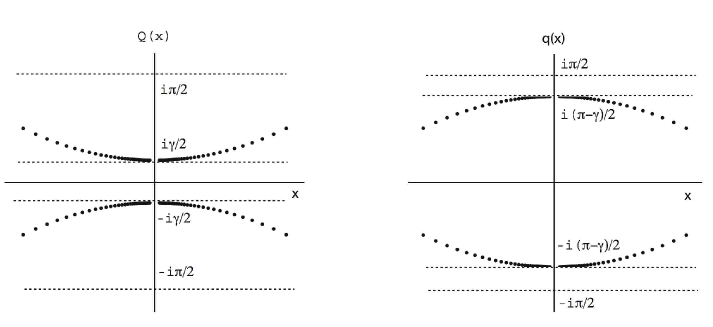
Figure 3: Schematic depiction of zeros of $Q(x)$ and $q(x)$, respectively

Since $Q(x)$ can have zeros near the real axis (namely, when $\gamma$ is close to zero), it is convenient to work instead with the shifted quantity $q(x)$ defined by

$$q(x)=Q\left(x+{i\pi\over{2}}\right)\,,$$ (3.10)

which is ANZ near the real axis. Also, one can check numerically that $T_{1}(x)$ and $T_{2}(x)$ do not have zeros near the real axis except for a simple zero at the origin. To remove this root, we define

$$\check{T}_{1}(x)={T_{1}(x)\over\mu(x)}\,,\qquad\check{T}_{2}(x)={T_{2}(x)\over\mu(x)}\,,$$ (3.11)

where again $\mu(x)$ is any function whose only real root is a simple zero at the origin, in particular $\mu(0)=0\,,\ \mu^{\prime}(0)\neq 0$, so that $\check{T}_{1}(x)$ and $\check{T}_{2}(x)$ are ANZ when $x$ is near the real axis.

3.2 Auxiliary functions

It is convenient to define the auxiliary functions [25]

$$b(x)={\lambda_{1}(x)+\lambda_{2}(x)\over{\lambda_{3}(x)}}\,,\qquad{\bar{b}}(x)={\lambda_{3}(x)+\lambda_{2}(x)\over{\lambda_{1}(x)}}=b(-x)\,.$$ (3.12)

Since $\bar{b}(x)$ is the complex conjugate of $b(x)$ for real $x$, we shall generally refrain from writing equations for $\bar{b}(x)$, as they can be readily obtained by conjugation of corresponding equations for $b(x)$. With the help of (3.6), we obtain

$$b(x) = {[l_{1}(x-{i\gamma\over{2}})+l_{2}(x-{i\gamma\over{2}})]l_{2}(x+{i\gamma\over{2}})\over{l_{1}(x-{i\gamma\over{2}})l_{1}(x+{i\gamma\over{2}})}}$$

$$= {T_{1}(x-{i\gamma\over{2}})\over{\sinh(2x+2i\gamma)}}{\phi(x-{i\gamma\over{2}})\over{\phi(x+{i\gamma\over{2}})\phi(x+{3i\gamma\over{2}})}}{B^{(+)}(x+{i\gamma\over{2}})\over{B^{(-)}(x-{i\gamma\over{2}})B^{(-)}(x+{i\gamma\over{2}})}}{Q(x+{3i\gamma\over{2}})\over{Q(x-{3i\gamma\over{2}})}}\,.$$

In terms of the quantities (3.10), (3.11), we rewrite this relation in the compact form

$$b(x)=C_{b}(x)\,\check{T}_{1}(x-{i\gamma\over{2}}){q(x+{3i\gamma\over{2}}-{i\pi\over 2})\over{q(x-{3i\gamma\over{2}}+{i\pi\over 2})}}\,,$$ (3.14)

with

$$C_{b}(x) = {\mu(x-{i\gamma\over{2}})\phi(x-{i\gamma\over{2}})\over{\sinh(2x+2i\gamma)\phi(x+{i\gamma\over{2}})\phi(x+{3i\gamma\over{2}})}}{B^{(+)}(x+{i\gamma\over{2}})\over{B^{(-)}(x-{i\gamma\over{2}})B^{(-)}(x+{i\gamma\over{2}})}}\,.$$ (3.15)

Defining

$$B(x)=1+b(x)\,,\qquad{\bar{B}}(x)=1+{\bar{b}}(x)=B(-x)\,,$$ (3.16)

we also obtain

$$T_{2}(x)=\lambda_{3}(x)\,B(x)=\lambda_{1}(x)\,{\bar{B}}(x)\,.$$ (3.17)

In terms of the quantities (3.10), (3.11), we can reexpress (3.17) as

$$\check{T}_{2}(x) = t_{-}(x)\,{q(x-{3i\gamma\over{2}}+{i\pi\over{2}})\over{q(x+{i\gamma\over{2}}-{i\pi\over{2}})}}B(x)\,,$$ (3.18)

$$= t_{+}(x)\,{q(x+{3i\gamma\over{2}}-{i\pi\over{2}})\over{q(x-{i\gamma\over{2}}+{i\pi\over{2}})}}{\bar{B}}(x)\,,$$ (3.19)

with

$$t_{\pm}(x)={\sinh(2x\mp 2i\gamma)\over\mu(x)}B^{(\pm)}(x-{i\gamma\over{2}})B^{(\pm)}(x+{i\gamma\over{2}})\phi(x\mp{3i\gamma\over{2}})\phi(x\mp{i\gamma\over{2}}).$$ (3.20)

We note that $B(x)$ has zeros just above the real axis, and $\bar{B}(x)$ has zeros just below the real axis. Indeed, due to the factor $Q(x+\frac{i\gamma}{2})$ in the definition of $\lambda_{3}(x)$ (3.2), and the fact that the imaginary parts of the Bethe roots have magnitude $>\frac{\gamma}{2}$, we see that $\lambda_{3}(x)$ has poles just above the real axis (and also just below the line $\Im m\,x=-\gamma$). It follows from (3.17) that $B(x)$ must have corresponding zeros to cancel these poles, since the product $\lambda_{3}(x)B(x)=T_{2}(x)$ is analytic. Similarly, since $\lambda_{1}(x)$ has poles just below the real axis (and also just above the line $\Im m\,x=\gamma$), $\bar{B}(x)$ has corresponding zeros to cancel these poles.

Finally, we define the auxiliary functions $y(x)$ and $Y(x)$,

$$y(x)={T_{0}(x)\,T_{2}(x)\over f(x)}\,,\qquad Y(x)=1+y(x)\,,$$ (3.21)

in terms of which the fusion relation (3.4) becomes

$$\check{T}_{1}(x-{i\gamma\over{2}})\,\check{T}_{1}(x+{i\gamma\over{2}})={f(x)\,Y(x)\over\mu(x-{i\gamma\over{2}})\,\mu(x+{i\gamma\over{2}})}\,.$$ (3.22)

3.3 Derivation of NLIE

Since $\ln\check{T}_{2}(x)$ is analytic near the real axis, Cauchy’s theorem gives

$$0=\oint_{C}dx\ [\ln\check{T}_{2}(x)]^{\prime\prime}e^{ikx}=\int_{C_{1}}[\ln\check{T}_{2}(x)]^{\prime\prime}e^{ikx}dx+\int_{C_{2}}[\ln\check{T}_{2}(x)]^{\prime\prime}e^{ikx}dx\,,$$ (3.23)

where we choose the contour $C$ as in Figure 2, with $\epsilon$ such that max $\{y_{k}\}-\frac{\gamma}{2}<\epsilon$. These integrals can be written using (3.18) and (3.19) as

$$\int_{C_{1}}[\ln\check{T}_{2}(x)]^{\prime\prime}e^{ikx}dx = \int_{C_{1}}dx\ \left\{\ln t_{-}(x)\right\}^{\prime\prime}e^{ikx}+\int_{C_{1}}dx\ \left\{\ln\left[{q(x-\frac{3i\gamma}{2}+\frac{i\pi}{2})\over q(x+\frac{i\gamma}{2}-\frac{i\pi}{2})}\right]\right\}^{\prime\prime}e^{ikx}$$ (3.24)

$$+ \int_{C_{1}}dx\ \left\{\ln B(x)\right\}^{\prime\prime}e^{ikx}\,,$$

$$\int_{C_{2}}[\ln\check{T}_{2}(x)]^{\prime\prime}e^{ikx}dx = \int_{C_{2}}dx\ \left\{\ln t_{+}(x)\right\}^{\prime\prime}e^{ikx}+\int_{C_{2}}dx\ \left\{\ln\left[{q(x+\frac{3i\gamma}{2}-\frac{i\pi}{2})\over q(x-\frac{i\gamma}{2}+\frac{i\pi}{2})}\right]\right\}^{\prime\prime}e^{ikx}$$ (3.25)

$$+ \int_{C_{2}}dx\ \left\{\ln\bar{B}(x)\right\}^{\prime\prime}e^{ikx}\,,$$

so that the quantities $q(x+\frac{i\gamma}{2}-\frac{i\pi}{2})$ and $q(x-\frac{i\gamma}{2}+\frac{i\pi}{2})$ are integrated along $C_{1}$ and $C_{2}$, respectively, and not the other way around.

In terms of Fourier transforms defined by (2.15), we can rewrite (3.24) and (3.25) as

$$\widehat{{\cal L}\check{T}^{\prime\prime}_{2}}(k) = \widehat{{\cal L}t^{\prime\prime}_{-}}(k)+\left[e^{\left({\gamma\over{2}}-{\pi\over{2}}\right)k}-e^{\left({\pi\over{2}}-{3\gamma\over{2}}\right)k}\right]\widehat{Lq^{\prime\prime}}(k)+\widehat{{\cal L}B^{\prime\prime}}(k)\,,$$ (3.26)

$$\widehat{L\check{T}^{\prime\prime}_{2}}(k) = \widehat{Lt^{\prime\prime}_{+}}(k)+\left[e^{\left({3\gamma\over{2}}-{\pi\over{2}}\right)k}-e^{\left({\pi\over{2}}-{\gamma\over{2}}\right)k}\right]\widehat{Lq^{\prime\prime}}(k)+\widehat{L{\bar{B}}^{\prime\prime}}(k)\,,$$ (3.27)

respectively. In obtaining these results, we use the periodicity of $q(x)$ as in (2.17) to make the imaginary part of the argument negative.

Adding (3.26) and (3.27), and remembering the fact (3.23)

$$\widehat{{\cal L}\check{T}^{\prime\prime}_{2}}(k)+\widehat{L\check{T}^{\prime\prime}_{2}}(k)=0\,,$$ (3.28)

we obtain an expression for $\widehat{Lq^{\prime\prime}}(k)$,

$$\left[e^{\left({\pi\over{2}}-{3\gamma\over{2}}\right)k}-e^{\left({\gamma\over{2}}-{\pi\over{2}}\right)k}-e^{\left({3\gamma\over{2}}-{\pi\over{2}}\right)k}+e^{\left({\pi\over{2}}-{\gamma\over{2}}\right)k}\right]\widehat{Lq^{\prime\prime}}(k)=\widehat{L{\bar{B}}^{\prime\prime}}(k)+\widehat{{\cal L}B^{\prime\prime}}(k)+D_{q}(k)\,,$$ (3.29)

where we define

$$D_{q}(k)=\widehat{Lt^{\prime\prime}_{+}}(k)+\widehat{{\cal L}t^{\prime\prime}_{-}}(k)\,.$$ (3.30)

From the expression (3.14) for $b(x)$ and the fact that $\check{T}_{1}(x)$ is ANZ near the real axis, we obtain

$$\widehat{Lb^{\prime\prime}}(k) = e^{-\frac{\gamma k}{2}}\widehat{L\check{T}^{\prime\prime}_{1}}(k)+\widehat{Lq^{\prime\prime}}(k)\left[e^{\left({3\gamma\over{2}}-{\pi\over{2}}\right)k}-e^{\left({\pi\over{2}}-{3\gamma\over{2}}\right)k}\right]+\widehat{LC^{\prime\prime}_{b}}(k)\,.$$ (3.31)

From the fusion relation (3.22), we obtain

$$\left(e^{{\gamma k\over{2}}}+e^{-{\gamma k\over{2}}}\right)\widehat{L\check{T}^{\prime\prime}_{1}}(k)=\widehat{LY^{\prime\prime}}(k)+\widehat{Lf^{\prime\prime}}(k)-\left(e^{\gamma k\over 2}+e^{-{\gamma k\over 2}}\right)\widehat{L\mu^{\prime\prime}}(k)+e^{\gamma k\over 2}\delta(k)\,,$$ (3.32)

where $\delta(k)$ is again given by (B.3). Substituting Eqs.(3.29) and (3.32) into Eq.(3.31), we obtain

$$\widehat{Lb^{\prime\prime}}(k) = {e^{\left({3\gamma\over{2}}-{\pi\over{2}}\right)k}-e^{\left({\pi\over{2}}-{3\gamma\over{2}}\right)k}\over{e^{\left({\pi\over{2}}-{3\gamma\over{2}}\right)k}-e^{\left({\gamma\over{2}}-{\pi\over{2}}\right)k}-e^{\left({3\gamma\over{2}}-{\pi\over{2}}\right)k}+e^{\left({\pi\over{2}}-{\gamma\over{2}}\right)k}}}\left[\widehat{L{\bar{B}}^{\prime\prime}}(k)+\widehat{{\cal L}B^{\prime\prime}}(k)+D_{q}(k)\right]$$ (3.33)

$$+ {e^{-{\gamma k\over{2}}}\over{e^{{\gamma k\over{2}}}+e^{-{\gamma k\over{2}}}}}\left[\widehat{LY^{\prime\prime}}(k)+\widehat{Lf^{\prime\prime}}(k)\right]+\widehat{LC^{\prime\prime}_{b}}(k)-e^{-{\gamma k\over 2}}\widehat{L\mu^{\prime\prime}}(k)+{\delta(k)\over e^{\gamma k\over 2}+e^{-{\gamma k\over 2}}}$$

$$= -\widehat{G}(k)\left[\widehat{L{\bar{B}}^{\prime\prime}}(k)+\widehat{{\cal L}B^{\prime\prime}}(k)\right]+\widehat{G}_{2}(k)\,\widehat{LY^{\prime\prime}}(k)+C(k)\,,$$

where

$$\widehat{G}(k) = {\sinh\left((\pi-3\gamma)\frac{k}{2}\right)\over 2\cosh{\gamma k\over{2}}\sinh\left((\pi-2\gamma)\frac{k}{2}\right)}\,,$$ (3.34)

$$\widehat{G}_{2}(k) = {e^{-{\gamma k\over{2}}}\over{e^{{\gamma k\over{2}}}+e^{-{\gamma k\over{2}}}}}\,,$$ (3.35)

$$C(k) = -\widehat{G}(k)\,D_{q}(k)+\widehat{G}_{2}(k)\,\widehat{Lf^{\prime\prime}}(k)+\widehat{LC^{\prime\prime}_{b}}(k)-e^{-{\gamma k\over 2}}\widehat{L\mu^{\prime\prime}}(k)+{\delta(k)\over e^{\gamma k\over 2}+e^{-{\gamma k\over 2}}}\,.$$ (3.36)

We find that $C(k)$ is given by (B.11)

$$C(k) = 2\pi k\Bigg{\{}N\left({e^{i\Lambda k}+e^{-i\Lambda k}\over{2\cosh{\gamma k\over{2}}}}\right)+{\left[\sinh\left((\eta_{+}-{\pi\over{2}})k\right)+\sinh\left((\eta_{-}-{\pi\over{2}})k\right)\right]\over{2\cosh{\gamma k\over{2}}\sinh\left(({\pi\over{2}}-\gamma)k\right)}}$$ (3.37)

$$+ {\cosh\frac{\gamma k}{4}\sinh\left((3\gamma-\pi)\frac{k}{4}\right)\over\cosh\frac{\gamma k}{2}\sinh\left((2\gamma-\pi)\frac{k}{4}\right)}\Bigg{\}}\,.$$

We now turn to the third and final NLIE equation. From the definitions of $y(x)$ (3.21) and $\check{T}_{2}(x)$ (3.11), we obtain

$$\widehat{Ly^{\prime\prime}}(k)=\widehat{L\check{T}^{\prime\prime}_{2}}(k)+\widehat{LT^{\prime\prime}_{0}}(k)+\widehat{L\mu^{\prime\prime}}(k)-\widehat{Lf^{\prime\prime}}(k)\,.$$ (3.38)

To evaluate $\widehat{L\check{T}^{\prime\prime}_{2}}(k)$, we combine Eqs. (3.26) and (3.27) to cancel $\widehat{Lq^{\prime\prime}}(k)$, namely,

$$-e^{{\gamma k\over{2}}}\widehat{{\cal L}\check{T}^{\prime\prime}_{2}}(k)+e^{-{\gamma k\over{2}}}\widehat{L\check{T}^{\prime\prime}_{2}}(k)\,,$$

which together with (3.28) gives

$$\left(e^{{\gamma k\over{2}}}+e^{-{\gamma k\over{2}}}\right)\widehat{L\check{T}^{\prime\prime}_{2}}(k)=e^{-{\gamma k\over{2}}}\widehat{L{\bar{B}}^{\prime\prime}}(k)-e^{{\gamma k\over{2}}}\widehat{{\cal L}B^{\prime\prime}}(k)+D_{T}(k)\,,$$ (3.39)

where we define

$$D_{T}(k)=e^{-{\gamma k\over{2}}}\widehat{Lt^{\prime\prime}_{+}}(k)-e^{{\gamma k\over{2}}}\widehat{{\cal L}t^{\prime\prime}_{-}}(k)\,.$$ (3.40)

Substituting the result (3.39) for $\widehat{L\check{T}^{\prime\prime}_{2}}(k)$ into (3.38), we obtain

$$\widehat{Ly^{\prime\prime}}(k)=-\widehat{G}_{2}(-k)\,\widehat{{\cal L}B^{\prime\prime}}(k)+\widehat{G}_{2}(k)\,\widehat{L{\bar{B}}^{\prime\prime}}(k)+C_{y}(k)\,,$$ (3.41)

where we define

$$C_{y}(k)={D_{T}(k)\over{e^{{\gamma k\over{2}}}+e^{-{\gamma k\over{2}}}}}+\widehat{LT^{\prime\prime}_{0}}(k)+\widehat{L\mu^{\prime\prime}}(k)-\widehat{Lf^{\prime\prime}}(k)\,.$$ (3.42)

We find (B.13)

$$C_{y}(k)=4\pi k\widehat{G}_{2}(-k)\,.$$ (3.43)

In summary, the NLIEs of the lattice SSG model with Dirichlet boundary conditions in Fourier space are

$$\widehat{Lb^{\prime\prime}}(k) = -\widehat{G}(k)\left[\widehat{L{\bar{B}}^{\prime\prime}}(k)+\widehat{{\cal L}B^{\prime\prime}}(k)\right]+\widehat{G}_{2}(k)\,\widehat{LY^{\prime\prime}}(k)+C(k)\,,$$ (3.44)

$$\widehat{Ly^{\prime\prime}}(k) = \widehat{G}_{2}(k)\,\widehat{L{\bar{B}}^{\prime\prime}}(k)-\widehat{G}_{2}(-k)\,\widehat{{\cal L}B^{\prime\prime}}(k)+C_{y}(k)\,,$$ (3.45)

where $C(k)$ and $C_{y}(k)$ are given by Eqs. (3.37) and (3.43), respectively. Passing to coordinate space, integrating twice, and taking the continuum limit, we obtain

$$\ln\mathsf{b}(\theta) = \int_{-\infty}^{\infty}d\theta^{\prime}\ \mathsf{G}(\theta-\theta^{\prime}-i\varepsilon)\ln\mathsf{B}(\theta^{\prime}+i\varepsilon)-\int_{-\infty}^{\infty}d\theta^{\prime}\ \mathsf{G}(\theta-\theta^{\prime}+i\varepsilon)\ln\bar{}\mathsf{B}(\theta^{\prime}-i\varepsilon)$$

$$+ \int_{-\infty}^{\infty}d\theta^{\prime}\ \mathsf{G}_{2}(\theta-\theta^{\prime}+i\varepsilon)\ln\mathsf{Y}(\theta^{\prime}-i\varepsilon)+i2mL\sinh\theta+i\,\mathsf{P}_{bdry}(\theta)-i\pi\,,$$

$$\ln\bar{}\mathsf{b}(\theta) = -\int_{-\infty}^{\infty}d\theta^{\prime}\ \mathsf{G}(\theta-\theta^{\prime}-i\varepsilon)\ln\mathsf{B}(\theta^{\prime}+i\varepsilon)+\int_{-\infty}^{\infty}d\theta^{\prime}\ \mathsf{G}(\theta-\theta^{\prime}+i\varepsilon)\ln\bar{}\mathsf{B}(\theta^{\prime}-i\varepsilon)$$

$$+ \int_{-\infty}^{\infty}d\theta^{\prime}\ \mathsf{G}_{2}(\theta^{\prime}-\theta+i\varepsilon)\ln\mathsf{Y}(\theta^{\prime}+i\varepsilon)-i2mL\sinh\theta-i\,\mathsf{P}_{bdry}(\theta)+i\pi\,,$$

$$\ln\mathsf{y}(\theta) = \int_{-\infty}^{\infty}d\theta^{\prime}\ \mathsf{G}_{2}(\theta-\theta^{\prime}+i\varepsilon)\ln\bar{}\mathsf{B}(\theta^{\prime}-i\varepsilon)+\int_{-\infty}^{\infty}d\theta^{\prime}\ \mathsf{G}_{2}(\theta^{\prime}-\theta+i\varepsilon)\ln\mathsf{B}(\theta^{\prime}+i\varepsilon)$$ (3.46)

$$+ i\,\mathsf{P}_{y}(\theta)\,.$$

As in the spin-1/2 case, the continuum limit consists of taking $\Lambda\rightarrow\infty$, $N\rightarrow\infty$ and lattice spacing $a\rightarrow 0$, such that the interval length $L\equiv x_{+}-x_{-}$ and the soliton mass $m$ are given by (2.33). The renormalized rapidity $\theta$ is again given by (2.34), and we have defined $\mathsf{b}(\theta)=b(\frac{\gamma\theta}{\pi})$, etc. as in (2.36). Hence, the kernel $\mathsf{G}(\theta)$ is given by

$$\mathsf{G}(\theta)={\gamma\over 2\pi^{2}}\int_{-\infty}^{\infty}dk\ e^{-ik\gamma\theta/\pi}\ \widehat{G}(k)\,,$$ (3.47)

where $\widehat{G}(k)$ is given by (3.34); and $\mathsf{G}_{2}(\theta)$ is defined similarly in terms of $\widehat{G}_{2}(k)$ (3.35),

$$\mathsf{G}_{2}(\theta)={\gamma\over 2\pi^{2}}\int_{-\infty}^{\infty}dk\ e^{-ik\gamma\theta/\pi}\ \widehat{G}_{2}(k)={i\over 2\pi\sinh\theta}\,,$$ (3.48)

where $\theta$ has a slightly positive imaginary part. Finally, $\mathsf{P}_{bdry}(\theta)$ is given by

$$\mathsf{P}_{bdry}(\theta)=\int_{0}^{\frac{\gamma\theta}{\pi}}dx^{\prime}\,R(x^{\prime})=\frac{1}{2}\int_{-\frac{\gamma\theta}{\pi}}^{\frac{\gamma\theta}{\pi}}dx^{\prime}\,R(x^{\prime})={\gamma\over 4\pi^{2}}\int_{-\theta}^{\theta}d\theta^{\prime}\int_{-\infty}^{\infty}dk\ e^{-ik\gamma\theta^{\prime}/\pi}\ \hat{R}(k)\,,$$ (3.49)

where $\hat{R}(k)$ is given by

$$\hat{R}(k)=2\pi\Bigg{\{}{\left[\sinh\left((\eta_{+}-{\pi\over{2}})k\right)+\sinh\left((\eta_{-}-{\pi\over{2}})k\right)\right]\over{2\cosh{\gamma k\over{2}}\sinh\left((\pi-2\gamma)\frac{k}{2}\right)}}+{\cosh\frac{\gamma k}{4}\sinh\left((3\gamma-\pi)\frac{k}{4}\right)\over\cosh\frac{\gamma k}{2}\sinh\left((2\gamma-\pi)\frac{k}{4}\right)}\Bigg{\}}\,;$$ (3.50)

and $\mathsf{P}_{y}(\theta)$ is given by

$$\mathsf{P}_{y}(\theta)=4\pi\int_{-\infty}^{\theta}d\theta^{\prime}\ \mathsf{G}_{2}(-\theta^{\prime})=-2i\ln\tanh\frac{\theta}{2}-2\pi\,,$$ (3.51)

where $\theta$ has a slightly negative imaginary part. The integration constants are explained in Section C.2.

These NLIE equations are similar to those for the periodic chain [23, 25, 28], with additional boundary terms involving $\mathsf{P}_{bdry}(\theta)$ or $\mathsf{P}_{y}(\theta)$. These terms constitute one of our main results. As we shall see, these boundary terms make essential contributions to the boundary $S$ matrix (IR limit) and to the effective central charge (UV limit).

3.4 Vacuum and Casimir energies

The energy computation is similar to the one for the spin-1/2 case in Section 2.3. We see from (3.21) that $T_{2}(x)$ can be expressed in terms of $y(x)$,

$$T_{2}(x)={f(x)\,y(x)\over T_{0}(x)}\,.$$ (3.52)

It follows from the energy definition (3.7) together with the fact (2.39) that

$$E=-\frac{g}{a}\int\frac{dk}{2\pi}\left[e^{-ik(\Lambda+\frac{i\gamma}{2})}-e^{-ik(\Lambda-\frac{i\gamma}{2})}\right]\left[\widehat{Lf^{\prime}}(k)+\widehat{Ly^{\prime}}(k)-\widehat{LT^{\prime}_{0}}(k)\right]\,.$$ (3.53)

Recalling the results for $\widehat{Lf^{\prime\prime}}(k)$ (B.9) and $\widehat{Ly^{\prime\prime}}(k)$ (3.45), we obtain

$$E = -\frac{g}{a}\int\frac{dk}{2\pi}e^{-ik\Lambda}\Bigg{\{}\widehat{L\phi^{\prime}}(k)(e^{\gamma k}-1)(e^{(\gamma-\pi)k}+e^{-2\gamma k})$$ (3.54)

$$+ 2\sinh\left({\gamma k\over{2}}\right)\Big{[}e^{-{\gamma k\over{2}}}\widehat{LB^{(+)^{\prime}}}(k)+e^{{\gamma k\over{2}}}\widehat{LB^{(-)^{\prime}}}(k)+4\pi i\widehat{G}_{2}(-k)$$

$$+ 2\pi\frac{\psi_{2}(k)}{(-ik)}\left(e^{-\gamma k}+e^{(\gamma-\frac{\pi}{2})k}-1\right)\Big{]}+\frac{1}{\cosh{\gamma k\over{2}}}\left[\widehat{L{\bar{B}}^{\prime}}(k)+\widehat{{\cal L}B^{\prime}}(k)\right]\Bigg{\}}\,.$$

The first term gives the bulk vacuum energy, which can be written explicitly as

$$E_{B}=\frac{2Ng}{ia}\int_{-\infty}^{\infty}dke^{-2i\Lambda k}{\sinh\frac{\gamma k}{2}\cosh\left((\frac{3\gamma}{2}-\frac{\pi}{2})k\right)\over\sinh\frac{\pi k}{2}}\,.$$ (3.55)

The second term gives (with the help of (B.10)) the boundary vacuum energy

$$E_{b} = \frac{2g}{ia}\int_{-\infty}^{\infty}dke^{-i\Lambda k}\sinh\left({\gamma k\over{2}}\right)\Bigg{\{}\frac{1}{\sinh{\pi k\over 2}}\left[\cosh\left((\eta_{+}-\frac{\gamma}{2}-\frac{\pi}{2})k\right)+(\eta_{+}\to\eta_{-})\right]$$ (3.56)

$$+ {e^{\frac{\gamma k}{2}}\over\cosh\frac{\gamma k}{2}}+\frac{e^{(\frac{\pi}{4}-\gamma)k}+e^{(\gamma-\frac{\pi}{4})k}-e^{\frac{\pi k}{4}}}{2\sinh{\pi k\over 4}}\Bigg{\}}\,,$$

and the third term gives the Casimir energy,

$$E_{C}=-\frac{g}{a}\int_{-\infty}^{\infty}\frac{dk}{2\pi}e^{-i\Lambda k}\frac{1}{\cosh{\gamma k\over{2}}}\left[\widehat{L{\bar{B}}^{\prime}}(k)+\widehat{{\cal L}B^{\prime}}(k)\right]\,.$$ (3.57)

In order to take the continuum limit, we adopt (as in the spin-1/2 case) the renormalization procedure of keeping only the (finite) terms that can be expressed in terms of the physical mass $m$ (2.33). We implement this procedure by closing the integral contours in the lower half plane, and selecting only the contribution from the residue at $k=-\frac{i\pi}{\gamma}$. Since the integrand in (3.55) is analytic at $k=-\frac{i\pi}{\gamma}$, the bulk energy vanishes,

$$E_{B}=0\,,$$ (3.58)

in agreement with known results (see, e.g., the second reference in [23]). We obtain from (3.56) that the boundary vacuum energy does not vanish, however, and is given by

$$E_{b}=m\,.$$ (3.59)

That is, each boundary contributes the vacuum energy $m/2$. Note that this result is independent of the boundary parameters. We shall present further support for this result in Section 6. Finally, we find that the Casimir energy (3.57) is given by

$$E_{C}=\frac{m}{2\pi}\Im m\int_{-\infty}^{\infty}d\theta\ \sinh(\theta-i\varepsilon)\ln\bar{}\mathsf{B}(\theta-i\varepsilon)\,.$$ (3.60)

4 Infrared limit

In this Section we analyze the IR limit $mL\rightarrow\infty$. In particular, we compute the SSG soliton boundary $S$ matrix (4.27), and show that it coincides with one proposed by Bajnok et al. [32]. In making this identification, we determine the “lattice $\leftrightarrow$ IR” relation for the boundary SSG parameters (4.25).

Before starting this computation, we note the relations among the three bulk SSG parameters (see Figure 1). Let $\lambda$ denote the IR bulk SSG parameter, and recall that $\beta$ and $\gamma$ are our UV and lattice bulk SSG parameters, respectively. (See Eqs. (1.1), (1.3).) The SSG soliton bulk $S$ matrix [22] has the product form $SG(\theta\,;\lambda)\otimes RSOS(\theta)$, where $SG(\theta\,;\lambda)$ is the SG soliton bulk $S$ matrix [1], and $RSOS(\theta)$ is the quantum-group restricted SG model bulk $S$ matrix [2]. The bulk “UV $\leftrightarrow$ IR” relation is given by [22],

$$\frac{2\pi}{\beta^{2}}-\frac{1}{2}=\lambda\,.$$ (4.1)

The bulk “lattice $\leftrightarrow$ IR” relation is given by

$$\frac{1}{\frac{\pi}{\gamma}-2}=\lambda\,.$$ (4.2)

This relation can be readily inferred from a comparison of the kernel $\widehat{G}(k)$ (3.34) with the integral representation of the SG soliton-soliton scattering amplitude $SG_{++}(\theta\,;\lambda)$,

$$\frac{1}{i}\frac{d}{d\theta}\ln SG_{++}(\theta\,;\lambda)=\int_{-\infty}^{\infty}dk\,e^{-ik\theta}\,{\sinh\left((\frac{1}{\lambda}-1)\frac{\pi k}{2}\right)\over 2\cosh\frac{\pi k}{2}\sinh\frac{\pi k}{2\lambda}}\,.$$ (4.3)

The relations (4.1), (4.2) imply the bulk “UV $\leftrightarrow$ lattice” relation

$$\beta^{2}=4\left(\pi-2\gamma\right)\,.$$ (4.4)

The condition $0<\beta^{2}<4\pi$ therefore implies $0<\gamma<\frac{\pi}{2}$. The free Fermion point $\lambda=1$ corresponds to $\gamma=\frac{\pi}{3}$. In the “repulsive” domain $\gamma\in(0\,,\frac{\pi}{3})$, the particle spectrum consists only of supersymmetric multiplets of solitons and antisolitons. In the “attractive” domain $\gamma\in(\frac{\pi}{3}\,,\frac{\pi}{2})$, the spectrum also includes bound states, namely, supersymmetric multiplets of breathers of mass [22]

$$m_{n}=2m\sin\left(\frac{n\pi}{2\lambda}\right)\,,\qquad n=1\,,2\,,\ldots\,,\lfloor\lambda\rfloor\,.$$ (4.5)

We turn now to the boundary theory. Let $\xi_{\pm}$ denote the IR boundary SSG parameters, and recall that $\varphi_{\pm}$ and $\eta_{\pm}$ are our UV and lattice boundary SSG parameters, respectively. (See Eqs. (1.6), (1.5).)

We define the boundary $S$ matrices (reflection factors) $R(\theta_{h}\,;\lambda\,,\xi_{\pm})$ for a soliton with mass $m$ and rapidity $\theta_{h}$ by the Yang equation for a single soliton on an interval of length $L\gg 1/m$,

$$e^{i2mL\sinh\theta_{h}}R(\theta_{h}\,;\lambda\,,\xi_{-})\,R(\theta_{h}\,;\lambda\,,\xi_{+})=1\,.$$ (4.6)

We shall compute these $S$ matrices by deriving a similar relation from the IR limit $mL\rightarrow\infty$ of the NLIE for a state of one hole with rapidity $\theta_{h}$,

$$\ln\mathsf{b}(\theta) = i2mL\sinh\theta+i\mathsf{P}_{bdry}(\theta)+i\chi(\theta-\theta_{h})+i\chi(\theta+\theta_{h})$$ (4.7)

$$+ \int_{-\infty}^{\infty}d\theta^{\prime}\ \mathsf{G}_{2}(\theta-\theta^{\prime}+i\varepsilon)\ln\mathsf{Y}(\theta^{\prime}-i\varepsilon)-i\pi\,,$$

$$\ln\mathsf{y}(\theta) = i\mathsf{P}_{y}(\theta)+ig_{y}(\theta-\theta_{h})+ig_{y}(\theta+\theta_{h})\,,$$ (4.8)

where $\chi(\theta)$ and $g_{y}(\theta)$ are the hole source terms [25, 28]

$$\chi(\theta)=2\pi\int_{0}^{\theta}d\theta^{\prime}\,\mathsf{G}(\theta^{\prime})\,,\qquad g_{y}(\theta)=-i\ln\tanh\frac{\theta}{2}+\frac{\pi}{2}\,,$$ (4.9)

and where, in the latter equation, $\theta$ has a slightly negative imaginary part. Indeed, since $\ln\mathsf{b}(\theta_{h})$ is $i\pi$ times an odd integer (see, e.g., [25, 28]), evaluating Eq. (4.7) at $\theta_{h}$ and exponentiating both sides gives

$$e^{i2mL\sinh\theta_{h}}\,e^{i\mathsf{P}_{bdry}(\theta_{h})+i\chi(2\theta_{h})+{\cal K}(\theta_{h})}=1\,,$$ (4.10)

where ${\cal K}(\theta)$ is the convolution term in (4.7),

$${\cal K}(\theta)\equiv\int_{-\infty}^{\infty}d\theta^{\prime}\ \mathsf{G}_{2}(\theta-\theta^{\prime}+i\varepsilon)\ln\mathsf{Y}(\theta^{\prime}-i\varepsilon)\,.$$ (4.11)

Comparing (4.10) with the Yang equation (4.6), we conclude that the product of boundary $S$ matrices is given by

$$R(\theta_{h}\,;\lambda\,,\xi_{-})\,R(\theta_{h}\,;\lambda\,,\xi_{+})=e^{i\mathsf{P}_{bdry}(\theta_{h})+i\chi(2\theta_{h})+{\cal K}(\theta_{h})}\,.$$ (4.12)

We evaluate first the factor $e^{{\cal K}(\theta_{h})}$ which, as we shall see, is the RSOS factor. To this end, we observe from (3.51), (4.8) and (4.9) that $\mathsf{y}(\theta)$ is given by

$$\mathsf{y}(\theta)=-\tanh^{2}\frac{\theta}{2}\tanh\frac{1}{2}(\theta-\theta_{h})\tanh\frac{1}{2}(\theta+\theta_{h})\,.$$ (4.13)

It follows that

$$\ln\mathsf{Y}(\theta)=\ln(1+\mathsf{y}(\theta))=\ln\left[{\cosh^{2}\frac{\theta_{h}}{2}\cosh\theta\over\cosh^{2}\frac{\theta}{2}\cosh\frac{1}{2}(\theta-\theta_{h})\cosh\frac{1}{2}(\theta+\theta_{h})}\right]\,.$$ (4.14)

The convolution term (4.11) is therefore given by

$${\cal K}(\theta)=\ln\cosh\frac{\theta_{h}}{2}+Q_{1}(\theta)-2Q_{2}(\theta)-Q_{2}(\theta-\theta_{h})-Q_{2}(\theta+\theta_{h})\,,$$ (4.15)

where [28]

$$Q_{1}(\theta) = \int_{-\infty}^{\infty}d\theta^{\prime}\ \mathsf{G}_{2}(\theta-\theta^{\prime}+i\varepsilon)\ln\cosh(\theta^{\prime}-i\varepsilon)=-\frac{i}{2}\tan^{-1}\sinh\theta+\frac{1}{2}\ln\cosh\theta\,,$$

$$Q_{2}(\theta) = \int_{-\infty}^{\infty}d\theta^{\prime}\ \mathsf{G}_{2}(\theta-\theta^{\prime}+i\varepsilon)\ln\cosh\frac{1}{2}(\theta^{\prime}-i\varepsilon)=-\frac{i}{2}\chi_{2}(\theta)+\frac{1}{2}\ln\cosh\frac{\theta}{2}\,,$$ (4.16)

with

$$\chi^{\prime}_{2}(\theta)=\int_{-\infty}^{\infty}dk\,e^{-ik\theta}{1\over 4\cosh^{2}\frac{\pi k}{2}}\,,\qquad\chi_{2}(0)=1\,.$$ (4.17)

It follows that

$${\cal K}(\theta_{h})=\frac{i}{2}\left[\chi_{2}(2\theta_{h})+2\chi_{2}(\theta_{h})-\tan^{-1}\sinh\theta_{h}\right]\,.$$ (4.18)

Differentiating with respect to $\theta_{h}$, and then making use of (4.17) and the Fourier transform result

$${1\over\cosh\theta}=\int_{-\infty}^{\infty}dk\,e^{-ik\theta}{1\over 2\cosh\frac{\pi k}{2}}\,,$$ (4.19)

we obtain

$${d\over d\theta_{h}}{\cal K}(\theta_{h})=\frac{i}{2}\left[2\chi^{\prime}_{2}(2\theta_{h})+2\chi^{\prime}_{2}(\theta_{h})-{1\over\cosh\theta_{h}}\right]=\frac{i}{4}\int_{-\infty}^{\infty}dk\,{e^{-2ik\theta_{h}}\over\cosh^{2}\frac{\pi k}{2}\cosh^{2}\pi k}\,.$$ (4.20)

Upon integrating, we conclude that

$$e^{{\cal K}(\theta_{h})}\sim P_{min}(\theta_{h})^{2}\,,$$ (4.21)

where $P_{min}(\theta)$ is a reflection factor of the boundary tricritical Ising model [31], whose integral representation is given by [39]

$$P_{min}(\theta)\sim\exp\left\{\frac{i}{8}\int_{0}^{\infty}{dt\over t}\,{\sin(2t\theta/\pi)\over\cosh^{2}\frac{t}{2}\cosh^{2}t}\right\}\,.$$ (4.22)

We stress that the boundary term $\mathsf{P}_{y}(\theta)$ in (4.8) is essential for obtaining this result. Since $\mathsf{P}_{y}(\theta)$ is independent of the boundary parameters, so is the result (4.21).

We turn now to the remaining factor $e^{i\mathsf{P}_{bdry}(\theta_{h})+i\chi(2\theta_{h})}$ in (4.12) which, as we shall see, is the sine-Gordon factor. Differentiating with respect to $\theta_{h}$, and recalling the Fourier transform results (3.34), (3.50), we obtain

$${d\over d\theta_{h}}\left[\mathsf{P}_{bdry}(\theta_{h})+\chi(2\theta_{h})\right]=\mathsf{P}^{\prime}_{bdry}(\theta_{h})+2\chi^{\prime}(2\theta_{h})$$ (4.23)

$$=\int_{-\infty}^{\infty}dk\,e^{-ik\theta_{h}}\Bigg{\{}{\left[\sinh\left((\eta_{+}-{\pi\over{2}})\frac{\pi k}{\gamma}\right)+\sinh\left((\eta_{-}-{\pi\over{2}})\frac{\pi k}{\gamma}\right)\right]\over{2\cosh{\pi k\over{2}}\sinh\left((\frac{\pi}{\gamma}-2)\frac{\pi k}{2}\right)}}$$

$$\qquad+2{\sinh\frac{3\pi k}{4}\sinh\left((\frac{\pi}{\gamma}-3)\frac{\pi k}{4})\right)\over\sinh\pi k\sinh\left((\frac{\pi}{\gamma}-2)\frac{\pi k}{4}\right)}\Bigg{\}}\,.$$

Let us compare this result with the soliton reflection amplitude $P_{+}(\theta\,,\xi)$ of the boundary SG model with Dirichlet boundary conditions [3], which has the integral representation [38]

$$\frac{1}{i}\frac{d}{d\theta}\ln P_{+}(\theta\,,\xi)=\int_{-\infty}^{\infty}dk\,e^{-ik\theta}\left[{\sinh\left((1+\frac{2\xi}{\pi\lambda})\frac{\pi k}{2}\right)\over 2\cosh\frac{\pi k}{2}\sinh\frac{\pi k}{2\lambda}}+{\sinh\frac{3\pi k}{4}\sinh\left((\frac{1}{\lambda}-1)\frac{\pi k}{4})\right)\over\sinh\pi k\sinh\frac{\pi k}{4\lambda}}\right]\,,$$ (4.24)

where $\lambda$ and $\xi$ are the bulk and boundary IR parameters, respectively. Recalling the bulk “lattice $\leftrightarrow$ IR” relation (4.2), and assuming the boundary “lattice $\leftrightarrow$ IR” relation

$$\eta_{\pm}=\frac{1}{2}(\pi+\gamma)+\left(1-\frac{2\gamma}{\pi}\right)\xi_{\pm}\,,$$ (4.25)

we conclude that

$$e^{i\mathsf{P}_{bdry}(\theta_{h})+i\chi(2\theta_{h})}=P_{+}(\theta_{h}\,,\xi_{-})\,P_{+}(\theta_{h}\,,\xi_{+})\,.$$ (4.26)

Combining the results (4.12), (4.21) and (4.26), we conclude that the NLIE generates the following SSG soliton boundary $S$ matrices

$$R(\theta_{h}\,;\lambda\,,\xi_{\pm})\sim P_{+}(\theta_{h}\,,\xi_{\pm})\,P_{min}(\theta_{h})\,.$$ (4.27)

This is the boundary $S$ matrix which was proposed by Bajnok et al. [32] for the the Dirichlet BSSG⁺ model. This is another of our main results. Similarly to the bulk case, the SSG boundary $S$ matrix is a product of SG and RSOS boundary $S$ matrices.

For general values of boundary parameters, the BSSG⁺ model with one boundary has the conserved supercharge [30, 31, 32]

$$\tilde{Q}_{+}=Q+\bar{Q}+\gamma^{\prime}\Gamma\,,$$ (4.28)

where $\Gamma=(-1)^{F}$ is the Fermionic parity operator, and $\gamma^{\prime}$ is an undetermined parameter. Bajnok et al. also propose the relation

$$\tilde{Q}_{+}^{2}=2\left(\tilde{H}+m\tilde{Z}\right)\,,$$ (4.29)

where $\tilde{H}$ is the Hamiltonian, and $\tilde{Z}$ is the topological charge. Since the ground state has $\tilde{Q}_{+}=\gamma^{\prime}$ and $\tilde{Z}=0$, it has energy $\tilde{H}=\gamma^{\prime 2}/2$. Our result (3.59) that each boundary contributes vacuum energy $m/2$ implies that

$$\gamma^{\prime}=\pm\sqrt{m}\,,$$ (4.30)

at least for the Dirichlet case. That is, we have succeeded to fix the undetermined parameter in the scattering theory proposed in [32].

5 Ultraviolet limit

In this Section we first analytically compute the Casimir energy $E_{C}(L)$ (3.60) in the UV limit $mL\rightarrow 0$. The result (5.26) is proportional to the effective central charge

$$E_{C}(0)=-\frac{\pi}{24L}c_{eff}(0)\,,$$ (5.1)

where $c_{eff}(0)=c-24\Delta_{0}$, $c$ is the central charge, and $\Delta_{0}$ is the $L_{0}$ eigenvalue of the ground state. We then compare this result for $c_{eff}(0)$ to the value for the conformal limit of the SSG model with Dirichlet boundary conditions. In this way, we obtain a boundary “UV $\leftrightarrow$ lattice” relation (5.31). When combined with the boundary “lattice $\leftrightarrow$ IR” relation from the previous section (4.25), we obtain the boundary “UV $\leftrightarrow$ IR” relation (5.32).

5.1 NLIE computation

We now proceed to analytically evaluate the Casimir energy in the UV limit $mL\rightarrow 0$. As is well known, only large values of $|\theta|$ contribute in this limit. Let us first consider $\theta\gg 1$, and define the finite rapidity $\hat{\theta}$ by

$$\theta=\hat{\theta}-\ln(mL)\,.$$ (5.2)

The corresponding contribution $E_{C}^{+}$ to the Casimir energy (3.60) is given by

$$L\,E_{C}^{+}=\frac{1}{16\pi}\int_{-\infty}^{\infty}d\hat{\theta}\,2ie^{\hat{\theta}}\left[\ln\mathsf{B}_{+}(\hat{\theta})-\ln\bar{}\mathsf{B}_{+}(\hat{\theta})\right]\,,$$ (5.3)

where the auxiliary functions $\mathsf{B}_{+}(\hat{\theta})\equiv\mathsf{B}(\hat{\theta}-\ln(mL))$, etc. satisfy the NLIE equations

$$\ln\mathsf{b}_{+}(\hat{\theta}) = \int_{-\infty}^{\infty}d\hat{\theta}^{\prime}\ \mathsf{G}(\hat{\theta}-\hat{\theta}^{\prime}-i\varepsilon)\ln\mathsf{B}_{+}(\hat{\theta}^{\prime}+i\varepsilon)-\int_{-\infty}^{\infty}d\hat{\theta}^{\prime}\ \mathsf{G}(\hat{\theta}-\hat{\theta}^{\prime}+i\varepsilon)\ln\bar{}\mathsf{B}_{+}(\hat{\theta}^{\prime}-i\varepsilon)$$

$$+ \int_{-\infty}^{\infty}d\hat{\theta}^{\prime}\ \mathsf{G}_{2}(\hat{\theta}-\hat{\theta}^{\prime}+i\varepsilon)\ln\mathsf{Y}_{+}(\hat{\theta}^{\prime}-i\varepsilon)+ie^{\hat{\theta}}+i\mathsf{P}_{bdry}(\infty)-i\pi\,,$$

$$\ln\bar{}\mathsf{b}_{+}(\hat{\theta}) = -\int_{-\infty}^{\infty}d\hat{\theta}^{\prime}\ \mathsf{G}(\hat{\theta}-\hat{\theta}^{\prime}-i\varepsilon)\ln\mathsf{B}_{+}(\hat{\theta}^{\prime}+i\varepsilon)+\int_{-\infty}^{\infty}d\hat{\theta}^{\prime}\ \mathsf{G}(\hat{\theta}-\hat{\theta}^{\prime}+i\varepsilon)\ln\bar{}\mathsf{B}_{+}(\hat{\theta}^{\prime}-i\varepsilon)$$ (5.4)

$$+ \int_{-\infty}^{\infty}d\hat{\theta}^{\prime}\ \mathsf{G}_{2}(\hat{\theta}^{\prime}-\hat{\theta}+i\varepsilon)\ln\mathsf{Y}_{+}(\hat{\theta}^{\prime}+i\varepsilon)-ie^{\hat{\theta}}-i\mathsf{P}_{bdry}(\infty)+i\pi\,,$$

$$\ln\mathsf{y}_{+}(\hat{\theta}) = \int_{-\infty}^{\infty}d\hat{\theta}^{\prime}\ \mathsf{G}_{2}(\hat{\theta}-\hat{\theta}^{\prime}+i\varepsilon)\ln\bar{}\mathsf{B}(\hat{\theta}^{\prime}-i\varepsilon)+\int_{-\infty}^{\infty}d\hat{\theta}^{\prime}\ \mathsf{G}_{2}(\hat{\theta}^{\prime}-\hat{\theta}+i\varepsilon)\ln\mathsf{B}(\hat{\theta}^{\prime}+i\varepsilon)\,,$$

which are independent of $mL$. The $\mathsf{P}_{y}$ term (3.51) does not appear in the third equation due to the fact $\mathsf{P}_{y}(\infty)=0\ \mbox{ mod }2\pi$. We note here for later reference that

$$\mathsf{P}_{bdry}(\infty)=\frac{1}{2}\hat{R}(0)=\frac{\pi}{\pi-2\gamma}\left(\eta_{+}+\eta_{-}-3\gamma\right)\,.$$ (5.5)

We use the so-called dilogarithm trick [6, 24]. We first rewrite the NLIE equations (5.4) in matrix form,

$$u=v+K*w\,,$$ (5.6)

where

$$u=\left(\begin{array}[]{c}\ln\mathsf{b}_{+}\\ \ln\bar{}\mathsf{b}_{+}\\ \ln\mathsf{y}_{+}\end{array}\right)\,,\quad v=\left(\begin{array}[]{c}ie^{\hat{\theta}}+i\mathsf{P}_{bdry}(\infty)-i\pi\\ -ie^{\hat{\theta}}-i\mathsf{P}_{bdry}(\infty)+i\pi\\ 0\end{array}\right)\,,\quad w=\left(\begin{array}[]{c}\ln\mathsf{B}_{+}\\ \ln\bar{}\mathsf{B}_{+}\\ \ln\mathsf{Y}_{+}\end{array}\right)\,,$$ (5.16)

the kernel $K$ is symmetric (i.e., $K_{ij}(\hat{\theta}\,,\hat{\theta}^{\prime})=K_{ji}(\hat{\theta}^{\prime}\,,\hat{\theta})$), and the star $*$ denotes convolution. We see from (5.6) that

$$\int_{-\infty}^{\infty}d\hat{\theta}\left(w^{T}u^{\prime}-w^{\prime T}u\right)=\int_{-\infty}^{\infty}d\hat{\theta}\left(w^{T}v^{\prime}-w^{\prime T}v\right)\,,$$ (5.17)

since the symmetry of the kernel implies that

$$\int_{-\infty}^{\infty}d\hat{\theta}\left(w^{T}K^{\prime}*w-w^{\prime T}K*w\right)=0\,.$$ (5.18)

It follows from (5.17) that

$$\int_{-\infty}^{\infty}d\hat{\theta}\,\Big{\{}(\ln\mathsf{b}_{+})^{\prime}\ln\mathsf{B}_{+}-\ln\mathsf{b}_{+}(\ln\mathsf{B}_{+})^{\prime}+(\ln\bar{}\mathsf{b}_{+})^{\prime}\ln\bar{}\mathsf{B}_{+}-\ln\bar{}\mathsf{b}_{+}(\ln\bar{}\mathsf{B}_{+})^{\prime}$$ (5.19)

$$+(\ln\mathsf{y}_{+})^{\prime}\ln\mathsf{Y}_{+}-\ln\mathsf{y}_{+}(\ln\mathsf{Y}_{+})^{\prime}\Big{\}}=\int_{-\infty}^{\infty}d\hat{\theta}\,2ie^{\hat{\theta}}\left(\ln\mathsf{B}_{+}-\ln\bar{}\mathsf{B}_{+}\right)$$

$$-i\left(e^{\hat{\theta}}+\mathsf{P}_{bdry}(\infty)-\pi\right)\left(\ln\mathsf{B}_{+}-\ln\bar{}\mathsf{B}_{+}\right)\Big{|}^{\hat{\theta}=\infty}_{\hat{\theta}=-\infty}\,.$$

Since $\mathsf{B}_{+}=1+\mathsf{b}_{+}$, etc., the LHS of (5.19) can be expressed in terms of the dilogarithm function $L_{+}(x)$, defined by

$$L_{+}(x)=\frac{1}{2}\int_{0}^{x}dy\left[\frac{1}{y}\ln(1+y)-\frac{1}{1+y}\ln y\right]\,.$$ (5.20)

The integral on the RHS of (5.19) is essentially the sought-after quantity $LE_{C}^{+}$ (5.3). We conclude that

$$L\,E_{C}^{+} = \frac{1}{8\pi}\Big{\{}L_{+}\left(\mathsf{b}_{+}(\infty)\right)-L_{+}\left(\mathsf{b}_{+}(-\infty)\right)+L_{+}\left(\bar{}\mathsf{b}_{+}(\infty)\right)-L_{+}\left(\bar{}\mathsf{b}_{+}(-\infty)\right)$$

$$+ L_{+}\left(\mathsf{y}_{+}(\infty)\right)-L_{+}\left(\mathsf{y}_{+}(-\infty)\right)+\frac{i}{2}\left(e^{\hat{\theta}}+\mathsf{P}_{bdry}(\infty)-\pi\right)\left(\ln\mathsf{B}_{+}-\ln\bar{}\mathsf{B}_{+}\right)\Big{|}^{\hat{\theta}=\infty}_{\hat{\theta}=-\infty}\Big{\}}\,.$$

The plateau values of the auxiliary functions can be obtained from the NLIE equations (5.4). For $\hat{\theta}\rightarrow\infty$, we readily obtain

$$\mathsf{b}_{+}(\infty)=\bar{}\mathsf{b}_{+}(\infty)=0\,,\qquad\mathsf{y}_{+}(\infty)=1\,.$$ (5.22)

To determine the plateau values for $\hat{\theta}\rightarrow-\infty$ is less trivial, as the corresponding plateau equations are nonlinear. We make the Ansatz

$$\mathsf{b}_{+}(-\infty)=e^{i\omega}\left(1+e^{i\omega}\right)\,,\quad\bar{}\mathsf{b}_{+}(-\infty)=e^{-i\omega}\left(1+e^{-i\omega}\right)\,,\quad\mathsf{y}_{+}(-\infty)=1+e^{i\omega}+e^{-i\omega}\,,$$ (5.23)

where $\omega$ is still to be determined. We indeed find a solution with

$$\omega=\frac{\mathsf{P}_{bdry}(\infty)-\pi}{2\left[\frac{3}{4}-\widehat{G}(0)\right]}=2\left(\eta_{+}+\eta_{-}-\gamma-\pi\right)\,,$$ (5.24)

where we have used the result (5.5). For the plateau values (5.23), the following sum rule holds [25]

$$L_{+}\left(\mathsf{b}_{+}(-\infty)\right)+L_{+}\left(\bar{}\mathsf{b}_{+}(-\infty)\right)+L_{+}\left(\mathsf{y}_{+}(-\infty)\right)-L_{+}(1)=\frac{\pi^{2}}{4}\,,\quad|\omega|<\frac{2\pi}{3}\,.$$ (5.25)

The above bound is satisfied when the boundary parameters are in the domain (3.9). Noting also that $L_{+}(0)=0$, we conclude that the Casimir energy is given by

$$L\,E_{C}(0)=2\,LE_{C}^{+}=-\frac{\pi}{24}\left[\frac{3}{2}-\frac{12}{\pi(\pi-2\gamma)}\left(\eta_{+}+\eta_{-}-\gamma-\pi\right)^{2}\right]\,.$$ (5.26)

In obtaining the first equality, we have used the fact that the contribution $E_{C}^{-}$ from $\theta\ll-1$ is the same as $E_{C}^{+}$, and that $E_{C}(0)=E_{C}^{+}+E_{C}^{-}$.

5.2 CFT analysis and UV-IR relation

Our result for the Casimir energy (5.26) together with the relation (5.1) evidently imply that the effective central charge has the value

$$c_{eff}(0)=c-24\Delta_{0}=\frac{3}{2}-\frac{12}{\pi(\pi-2\gamma)}\left(\eta_{+}+\eta_{-}-\gamma-\pi\right)^{2}\,.$$ (5.27)

We remark that for boundary parameter values $\eta_{+}=\eta_{-}=\frac{1}{2}(\pi+\gamma)$, the boundary terms in the Hamiltonian (1.5) which are proportional to $S^{z}$ vanish; and also $\Delta_{0}$ vanishes, so that $c_{eff}(0)=c=3/2$. A similar phenomenon was observed for the spin-1/2 case in [9].

In the UV limit, the boundary SSG model with Dirichlet boundary conditions (1.1), (1.6) evidently reduces to a system of one free Boson and one free Majorana Fermion, each with Dirichlet boundary conditions. For the former model, the central charge and lowest dimension are given by [40]

$$c_{B}=1\,,\qquad\Delta_{B}=\frac{1}{2\pi}\left(\varphi_{-}-\varphi_{+}\right)^{2}\,,$$ (5.28)

while for the latter model

$$c_{F}=\frac{1}{2}\,,\qquad\Delta_{F}=0\,.$$ (5.29)

It follows that the SSG model with Dirichlet boundary conditions should have

$$c=c_{B}+c_{F}=\frac{3}{2}\,,\qquad\Delta_{0}=\Delta_{B}+\Delta_{F}=\frac{1}{2\pi}\left(\varphi_{-}-\varphi_{+}\right)^{2}\,.$$ (5.30)

Comparing this CFT result with the NLIE result (5.27) and recalling the bulk “UV $\leftrightarrow$ lattice” relation (4.4), we obtain the boundary “UV $\leftrightarrow$ lattice” relation

$$\eta_{\pm}=\frac{1}{2}(\pi+\gamma)\pm\frac{\beta}{2}\varphi_{\pm}\,.$$ (5.31)

Combining this result with the boundary “lattice $\leftrightarrow$ IR” relation (4.25), we finally arrive at the SSG boundary “UV $\leftrightarrow$ IR” relation

$$\xi_{\pm}=\pm\frac{2\pi}{\beta}\varphi_{\pm}\,.$$ (5.32)

This is another of our main results.

The relation (5.32) is similar to the one found by Ghoshal and Zamolodchikov [3] for the SG model (namely, $\xi=\frac{4\pi}{\beta}\varphi_{0}$), and it can be understood in a similar way. Indeed, for the SSG model, it is also plausible to assume a linear relation between these parameters,

$$\xi_{\pm}=a+b\varphi_{\pm}\,.$$ (5.33)

When $\varphi_{\pm}=0$, the model has the symmetry $\varphi\mapsto-\varphi$; and, since the RSOS factor of the boundary $S$ matrix is proportional to the identity for BSSG⁺ [32], the soliton and antisoliton reflection amplitudes should be equal, which corresponds to $\xi_{\pm}=0$. Thus, $a=0$. Furthermore, as in the SG model, there are boundary bound states corresponding to poles of the boundary $S$ matrix at $\theta=i\nu_{n}$, where

$$\nu_{n}=\frac{\xi_{\pm}}{\lambda}-\frac{(2n+1)\pi}{2\lambda}\,,\quad n=0\,,1\,,\ldots.$$ (5.34)

Moreover, these states satisfy [32]

$$\tilde{Q}_{+}^{2}=2\left(\frac{\gamma^{\prime 2}}{2}+m\cos\nu_{n}+m\right)\,,$$ (5.35)

which is consistent with (4.29), since these states have $\tilde{Z}=1$. When $\varphi_{\pm}$ have the half-period values $\varphi_{\pm}=\pm\pi/\beta$ , the $n=0$ bound state should have the same $\tilde{Q}_{+}^{2}$ eigenvalue as the ground state. From (5.35), we see that this condition corresponds to $\nu_{0}=\pi$, which in turn implies $\xi_{\pm}=\pi(\lambda+\frac{1}{2})=2\pi^{2}/\beta^{2}$, as follows from (5.34) and the bulk UV-IR relation (4.1). It follows that $b=\pm 2\pi/\beta$, and so we recover the boundary UV-IR relation (5.32).

6 Intermediate volume and BCPT

For intermediate values of volume $l\equiv mL$, the Casimir energy cannot be computed analytically. Nevertheless, it is possible to solve the NLIEs (3.46) numerically by iteration, and evaluate the Casimir energy through (3.60). Two sample plots of $c_{eff}(l)\equiv-24LE_{C}(L)/\pi$ vs. $\ln l$ are shown in Figure 4. The numerical result for $c_{eff}(l)$ in the UV region $l\rightarrow 0$ coincides with the analytical result (5.27). Also, as expected, $c_{eff}(l)$ decreases monotonically to 0 as $l$ varies from the UV region to the IR region $l\rightarrow\infty$.

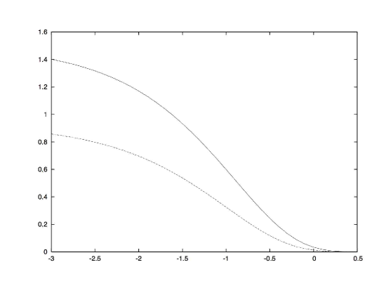
Figure 4: $c_{eff}$ vs. $\ln l$, for $\gamma=2\pi/7$, $\eta_{+}=\eta_{-}=(\pi+\gamma)/2$ (solid line) and $\eta_{+}=\eta_{-}=\pi/2+3\gamma/4$ (dotted line)

For small values of $l$, these numerical results can be compared with those from boundary conformal perturbation theory (BCPT). We shall follow closely the presentation in the Appendix of the second reference in [11]. We regard the SSG model (1.1) as a perturbed boundary CFT,

$$L=L_{BCFT}+L_{pertb}\,,\qquad L_{pertb}=-\frac{m_{0}}{2}\int_{0}^{L}dx\,\Phi(x,t)\,,$$ (6.1)

where $L_{BCFT}$ is the Lagrangian for a free scalar field $\varphi$ and a free Majorana Fermion field $\Psi$ obeying Dirichlet boundary conditions (1.6). We restrict our attention here to the particular case $\varphi_{-}=\varphi_{+}\equiv\varphi_{0}$, in order to avoid introducing boundary-changing operators. The bulk perturbing operator $\Phi(x,t)=\cos(\beta\varphi)\bar{\Psi}\Psi$ is a primary field with weights $(\Delta,\Delta)$, where

$$\Delta=\frac{1}{2}+\frac{\beta^{2}}{8\pi}\,,\qquad\frac{1}{2}<\Delta<1\,.$$ (6.2)

The corresponding Hamiltonian is

$$H(L)=H_{BCFT}+\frac{m_{0}}{2}\int_{0}^{L}dx\,\Phi(x,t)\,.$$ (6.3)

We map the infinitely long strip of width $L$ to the upper half plane by setting $z=e^{i\frac{\pi}{L}(x+t)}$, where $t=-iy$ is the Euclidean time. Taking the Hamiltonian at $t=0$ and changing the integration variable to $\theta=\frac{\pi}{L}x$, we have

$$H(L)=\frac{\pi}{L}\left(L_{0}-\frac{c}{24}\right)+\frac{m_{0}}{2}\left(\frac{\pi}{L}\right)^{2\Delta-1}\int_{0}^{\pi}d\theta\,\Phi(e^{i\theta},e^{-i\theta})\,,$$ (6.4)

with $c=3/2$. First-order perturbation theory implies that the ground-state energy is given by

$$E_{0}(L)=\frac{\pi}{L}\left(\Delta_{0}-\frac{c}{24}\right)+\frac{m_{0}}{2}\left(\frac{\pi}{L}\right)^{2\Delta-1}\int_{0}^{\pi}d\theta\,\langle 0|\Phi(e^{i\theta},e^{-i\theta})|0\rangle+O(m_{0}^{2})\,,$$ (6.5)

where $|0\rangle$ is the ground state of the unperturbed theory. Using the fact that the bulk one-point function has the form

$$\langle 0|\Phi(e^{i\theta},e^{-i\theta})|0\rangle=\frac{c_{bulk}}{(2\sin\theta)^{2\Delta}}\,,$$ (6.6)

and performing the $\theta$ integration, we obtain

$$E_{0}(L)=-\frac{\pi}{24L}c_{eff}(0)+\frac{m_{0}}{4}\left(\frac{\pi}{2L}\right)^{2\Delta-1}\frac{\Gamma(\frac{1}{2}-\Delta)\Gamma(\frac{1}{2})}{\Gamma(1-\Delta)}c_{bulk}+O(m_{0}^{2})\,,$$ (6.7)

where $c_{eff}(0)=c-24\Delta_{0}$, as before. The energy $E_{0}(L)$ is the sum of bulk, boundary and Casimir energies

$$E_{0}(L)=E_{B}L+E_{b}+E_{C}(L)\,,\qquad E_{C}(L)=-\frac{\pi}{24L}c_{eff}(l)\,.$$ (6.8)

Recalling the bulk and boundary energy results (3.58), (3.59), we obtain

$$c_{eff}(l)=c_{eff}(0)+\frac{24l}{\pi}-3m_{0}\left(\frac{\pi}{2L}\right)^{2\Delta-2}\frac{\Gamma(\frac{1}{2}-\Delta)\Gamma(\frac{1}{2})}{\Gamma(1-\Delta)}c_{bulk}+O(m_{0}^{2})\,.$$ (6.9)

Following Cardy and Lewellen [42], the coefficient of the bulk one-point function can be expressed as a ratio of scalar products,

$$c_{bulk}=\frac{\langle\!\langle\Phi|D\rangle}{\langle\!\langle 0|D\rangle}=\frac{\langle\!\langle\cos(\beta\varphi)|B_{D}(\varphi_{0})\rangle}{\langle 0,0|B_{D}(\varphi_{0})\rangle}\Big{|}_{c=1}\cdot\frac{\langle\!\langle\bar{\Psi}\Psi|\tilde{0}\rangle}{\langle\!\langle 0|\tilde{0}\rangle}\Big{|}_{\rm Ising}\,.$$ (6.10)

Here $|B_{D}(\varphi_{0})\rangle$ is the $c=1$ Dirichlet boundary state [40]

$$|B_{D}(\varphi_{0})\rangle={\cal N}_{D}\sum_{k=-\infty}^{\infty}e^{ik\beta\varphi_{0}}e^{-\sum_{n=1}^{\infty}\frac{1}{n}\alpha_{-n}\bar{\alpha}_{-n}}|0,k\rangle\,,$$ (6.11)

where $|0,k\rangle$ is annihilated by $\alpha_{n}$ and $\bar{\alpha}_{n}$ for $n>0$, and has weight $h_{0,k}=\frac{k^{2}\beta^{2}}{8\pi}$; and ${\cal N}_{D}$ is a normalization factor. Hence, $e^{\pm\beta\varphi}$ (which have weight $\frac{\beta^{2}}{8\pi}$) are identified with $|0,\pm 1\rangle$. Thus, $|\cos(\beta\varphi)\rangle\!\rangle=\frac{1}{2}\left(|0,1\rangle+|0,-1\rangle\right)$, and we conclude that

$$\frac{\langle\!\langle\cos(\beta\varphi)|B_{D}(\varphi_{0})\rangle}{\langle 0,0|B_{D}(\varphi_{0})\rangle}\Big{|}_{c=1}=\cos(\beta\varphi_{0})\,.$$ (6.12)

Moreover, $\bar{\Psi}\Psi=-\frac{1}{\pi}\varepsilon$, where $\varepsilon$ is the Ising energy density operator. Recalling the expressions [43] for the boundary states corresponding to fixed boundary conditions in terms of Ishibashi states

$$|\tilde{0}\rangle = \frac{1}{\sqrt{2}}|0\rangle\!\rangle+\frac{1}{\sqrt{2}}|\varepsilon\rangle\!\rangle+\frac{1}{\sqrt[4]{2}}|\sigma\rangle\!\rangle\,,$$

$$|\tilde{\frac{1}{2}}\rangle = \frac{1}{\sqrt{2}}|0\rangle\!\rangle+\frac{1}{\sqrt{2}}|\varepsilon\rangle\!\rangle-\frac{1}{\sqrt[4]{2}}|\sigma\rangle\!\rangle\,,$$ (6.13)

we obtain

$$\frac{\langle\!\langle\varepsilon|\tilde{0}\rangle}{\langle\!\langle 0|\tilde{0}\rangle}\Big{|}_{\rm Ising}=1\,.$$ (6.14)

We conclude from (6.10), (6.12) and (6.14) that the coefficient of the bulk one-point function is given by

$$c_{bulk}=-\frac{1}{\pi}\cos(\beta\varphi_{0})\,.$$ (6.15)

Moreover, the parameter $m_{0}$ is related to the SSG soliton mass $m$ by the so-called mass-gap formula [41]

$$m_{0}=\frac{8\Gamma(\Delta)}{\Gamma(1-\Delta)}\left[\frac{\pi m}{8}\left(\frac{2\Delta-1}{1-\Delta}\right)\right]^{2-2\Delta}\,.$$ (6.16)

This relation has the correct classical limit $\beta\rightarrow 0$, namely $m_{0}\rightarrow m_{1}$, where $m_{1}$ is the mass of the first breather (4.5).

Substituting (6.15) and (6.16) into (6.9), we obtain the result

$$c_{eff}(l)\approx c_{eff}(0)+\frac{24}{\pi}\left(l-\alpha_{1}\,l^{2-2\Delta}+\alpha_{2}\,l^{4-4\Delta}\right)\,,\qquad l\ll 1\,,$$ (6.17)

where

$$\alpha_{1}=-\left[\frac{2\Delta-1}{4(1-\Delta)}\right]^{2-2\Delta}\frac{\Gamma(\frac{1}{2}-\Delta)\Gamma(\frac{1}{2})\Gamma(\Delta)}{\Gamma(1-\Delta)^{2}}\cos(\beta\varphi_{0})\,.$$ (6.18)

We have not attempted to compute the second-order correction $\alpha_{2}$. In Table 1, we compare the analytical BCPT result for $\alpha_{1}$ (6.18) with results obtained by fitting numerical NLIE values for $c_{eff}(l)$ to the curve (6.17). The excellent agreement between the analytical and numerical values further supports the validity of our NLIE (3.46), as well as the boundary energy result (3.59) and the boundary “UV $\leftrightarrow$ lattice” relation (5.31).

	$\varphi_{0}=0$		$\varphi_{0}=0.1$		$\varphi_{0}=0.2$
$\pi/\gamma$	NLIE	BCPT	NLIE	BCPT	NLIE	BCPT
2.6	1.05337	1.05314	1.03813	1.0379	0.992871	0.992644
2.8	0.977854	0.977706	0.960355	0.960207	0.908481	0.908335
3	0.898947	0.898868	0.880187	0.880108	0.824691	0.82461
3.5	0.717426	0.717416	0.698197	0.698184	0.641543	0.641519
4	0.572666	0.572698	0.554784	0.5548	0.502248	0.502225
4.5	0.46177	0.461973	0.445794	0.445941	0.398955	0.398957
5	0.37713	0.377594	0.363094	0.363448	0.321985	0.322071

Table 1: Comparison of NLIE (numerical) and BCPT (analytical) results for $\alpha_{1}$, for various values of bulk and boundary parameters.

7 Discussion

We have proposed a set of nonlinear integral equations (3.46) to describe the boundary supersymmetric sine-Gordon model BSSG⁺ with Dirichlet boundary conditions on a finite interval (1.1), (1.6). In particular, we have found the boundary terms $\mathsf{P}_{bdry}(\theta)$ and $\mathsf{P}_{y}(\theta)$ which encode boundary effects. We have computed the corresponding boundary $S$ matrix (4.27), and found that it coincides with the one proposed by Bajnok et al. [32] for the Dirichlet BSSG⁺ model, with conserved supercharge (4.28) depending on a parameter $\gamma^{\prime}$. We have determined this parameter (4.30) by computing the boundary vacuum energy. We have also proposed a relation (5.32) between the (UV) parameters in the boundary conditions and the (IR) parameters in the boundary $S$ matrix. Moreover, we have demonstrated that the NLIEs can be solved numerically for intermediate values of $mL$, and we have found agreement with our analytical result (5.27) for the effective central charge in the UV limit and with boundary conformal perturbation theory (6.17), (6.18).

There are a number of related questions which remain to be addressed. While we have focused here primarily on the ground state, it should be interesting to study bulk (along the lines [28]) and also boundary excitations. It would also be interesting to formulate the TBA equations for this model, and compare the results with those from our NLIE.

Ultimately, we would like to extend this (Dirichlet) analysis of BSSG⁺ to the case of general integrable boundary conditions [30]. For this we would need the Bethe Ansatz solution of the open spin-1 XXZ quantum spin chain with general integrable boundary terms [34], which is currently under investigation.

It is not evident which integrable spin-1 model, if any, corresponds to the Dirichlet BSSG^- model. Indeed, the boundary terms (1.5) already correspond to the most general diagonal $c$-number solution of the boundary Yang-Baxter equation. Perhaps additional dynamical boundary degrees of freedom or impurities will be required. An interesting feature of BSSG^- is that, in contrast to BSSG⁺, the RSOS part of the boundary $S$ matrix [32] does depend on the boundary parameter. Therefore, the corresponding NLIE may have a $\mathsf{P}_{y}(\theta)$ term which also depends on the boundary parameters.

Another interesting problem is to identify the specific feature of the spin-1 models which leads, in the continuum limit, to supersymmetry. It may be possible to construct an integrable open spin-1 chain whose continuum limit is integrable but not supersymmetric, such as models considered in [29]. We hope to be able to address some of these questions in the future.

Appendix A Range of boundary parameters

We derive here the restrictions on the ranges of the boundary parameters given in the main text (2.10), (3.9).

A.1 Spin-$\frac{1}{2}$

Our argument depends on two assumptions. First, the imaginary part of $\ln\bar{a}(x)$ is monotonically increasing. Second, there should be no holes on the real axis (except for a single hole at the origin). The first assumption suffers from exceptions for some values of $\gamma$ if the system size is small. However, we regard this as a finite size effect and expect our assumption to be valid in the thermodynamic limit.

We consider first the repulsive regime $0<\gamma<\frac{\pi}{2}$. Let $0<a<\frac{\pi}{2}$. We then define two functions,

$$\vartheta_{-}(x,a)=\frac{1}{i}\ln(-\frac{\sinh(x-ia)}{\sinh(x+ia)})\,,\qquad\vartheta_{+}(x,a)=\frac{1}{i}\ln(\frac{\sinh(x-ia)}{\sinh(x+ia)})\,,$$

where we adopt the convention for the logarithm such that its imaginary part is restricted to $[-\pi\,,\pi)$. These functions are essentially the same but for the choice of phase (Figure 5).

Figure 5: The functions $\vartheta_{-}$ (left) and $\vartheta_{+}$ (right).

We choose the branch of $\vartheta_{-}(x,a)$ such that a branch cut line emerges from $ia$ and goes to positive infinity, and another line starts from $-ia$ and goes to negative infinity, as shown in Figure 6.

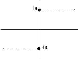
Figure 6: The branch cut lines for $\vartheta_{-}$.

In the rest of the range, $\frac{\pi}{2}<a<\pi$, we define

$$\vartheta_{-}(x,a)=-\vartheta_{-}(x,\pi-a)\,,\qquad\vartheta_{+}(x,a)=-\vartheta_{+}(x,\pi-a)\,.$$ (A.1)

Recalling (2.5), we consider

$$\frac{1}{i}{\rm Log}\,\bar{a}(x) =\sum_{\alpha=\pm}\vartheta_{-}(x,\frac{H_{\alpha}\gamma}{2})+\vartheta_{+}(2x,\gamma)+N\sum_{\alpha=\pm}\vartheta_{-}(x-\alpha\Lambda,\frac{\gamma}{2})$$

$$-\sum_{k=1}^{M}\left[\vartheta_{-}(x-v_{k},\gamma)+\vartheta_{-}(x+v_{k},\gamma)\right]\,,$$ (A.2)

where $M$ denotes the number of BAE roots. By Log, we mean the logarithm whose imaginary part is not restricted to $[-\pi,\pi)$. Strictly speaking, $\bar{a}$ is defined in the upper half-plane. We assume that it is also well-defined on the real axis. Note that $\frac{1}{i}{\rm Log}\,\bar{a}(0^{+})=\vartheta_{+}(0^{+},\gamma)=-\pi$ for $0<\gamma<\pi/2$.

With the help of the identities

$$\vartheta_{-}(\infty,a)=\pi-2a\,,\qquad\vartheta_{+}(\infty,a)=-2a\,,\qquad 0<a<\frac{\pi}{2}\,,$$

one easily derives the asymptotic value

$$\frac{1}{i\pi}{\rm Log}\,\bar{a}(\infty)=2(N-M+1)-\frac{\gamma}{\pi}(2N-4M+2+H_{+}+H_{-})$$ (A.3)

for $H_{\pm}$ in the in the interval (2.9). We denote the integer part of the above as $n$,

$$n=2(N-M+1)-\delta\,,$$

where

$$\delta=\lfloor\frac{\gamma}{\pi}(2N-4M+2+H_{+}+H_{-})\rfloor+1\,,$$

and $\lfloor x\rfloor$ specifies the integer part of $x$. When $x$ is a root or a hole, $\frac{1}{i\pi}{\rm Log}\,\bar{a}(x)$ is an odd integer. The range of $\frac{1}{i\pi}{\rm Log}\,\bar{a}$ is set so as to be able to accommodate $M$ roots. As already noted, there should be no holes (except for a single hole at the origin). Thanks to the assumption of monotonicity, these conditions determine the range of $n$ ,

$$2M-1\leq n<2M+1\,.$$ (A.4)

This is equivalent to having $\delta=2,3$. The ground state selects $M=N/2$, and this leads to the conclusion (2.10),

$$\frac{\pi}{\gamma}<H_{+}+H_{-}+2<\frac{3\pi}{\gamma}\,.$$

In the attractive regime $\pi/2<\gamma<\pi$, some functions in (A.2) must be rewritten in terms of $\tilde{\gamma}=\pi-\gamma$ which is now in the range $(0,\pi/2)$. Thanks to (A.1), this only results in an extra $2\pi$ on the RHS of (A.3). In this case, however, $\frac{1}{i}{\rm Log}\,\bar{a}(0^{+})=\pi$, which cancels this extra $2\pi$ in the argument for the possible values of $\delta$. We then reach the same conclusion on the range of $H_{\pm}$.

A.2 Spin-1

The spin-1 case suffers from an extra complication due to the absence of an auxiliary function which precisely encodes the “branch cut integers” such as $a$ and $\bar{a}$ in the spin-1/2 case. Previous studies [25, 28] nevertheless give this interpretation to $\ln b(x)$. It roughly encodes the information of the two-string center. We assume this here, and utilize $b$ in place of $\bar{a}$ in the above argument.

We consider first the repulsive regime, $0<\gamma<\frac{\pi}{3}$. The following representation is convenient for our purpose (recall Eqs. (3.1), (3.2)),

$$\Im m\,{\rm Log}\,b(x) =N\sum_{\alpha=\pm}\bigl{[}\vartheta_{-}(x-\alpha\Lambda,\frac{\gamma}{2})+\vartheta_{-}(x-\alpha\Lambda,\frac{3\gamma}{2})\bigr{]}$$

$$-\sum_{\alpha=\pm}\bigl{[}\vartheta_{-}(x,\eta_{\alpha}-\frac{\gamma}{2})+\vartheta_{-}(x,\eta_{\alpha}+\frac{\gamma}{2})\bigr{]}+\vartheta_{+}(2x,2\gamma)$$

$$-\sum_{k=1}^{M}\bigl{[}\vartheta_{-}(x-v_{k},\frac{\gamma}{2})+\vartheta_{-}(x+v_{k},\frac{\gamma}{2})+\vartheta_{-}(x-v_{k},\frac{3\gamma}{2})+\vartheta_{-}(x+v_{k},\frac{3\gamma}{2})\bigr{]}$$

$$+\Im m\,\ln(1+a_{1}(x-\frac{i\gamma}{2}))\,,$$ (A.5)

where we define $a_{1}(x)=l_{1}(x)/l_{2}(x)$. In the above, $\vartheta_{+}(2x,2\gamma)$ should be understood as $-\vartheta_{+}(2x,\pi-2\gamma)$ if $\pi/4<\gamma<\pi/3$. The above expression is valid for $\Im m\,x=+\epsilon$.

We assume that the ground state is given by a sea of 2-strings with slight deviations, $|{\Im}m\,v_{k}|=\gamma/2+\epsilon$, and $M=N$. Then a careful analysis concludes

$$\Im m\,\ln(1+a_{1}(x+i\epsilon-\frac{i\gamma}{2}))|_{x\rightarrow\infty}=\gamma-(\eta_{+}+\eta_{-})+\delta\pi\,,$$

where $\delta$ is an integer satisfying $|\gamma-(\eta_{+}+\eta_{-})+\delta\pi|<\pi$. This leads to the following expression of the asymptotic value,

$$\Im m\,{\rm Log}\,b(\infty)=3(\eta_{+}+\eta_{-}-\gamma)-4\pi+2\pi N+\delta\pi\,,$$

where, for simplicity, we have further restricted the boundary parameters to the interval $\pi/2<\eta_{\pm}<\pi-\gamma/2$.

For the spin-1 case, we must locate $N/2$ 2-string centers on the real positive $x$-axis. Then an argument similar to the one for the spin-1/2 case leads to

$$\pi<\eta_{+}+\eta_{-}-\gamma+\frac{\delta}{3}\pi<\frac{5\pi}{3}.$$

One can then easily draw a conclusion that $\delta=1$ is the only consistent choice, and that the constraint (3.9) must be imposed,

$$\frac{2\pi}{3}+\gamma<\eta_{+}+\eta_{-}<\frac{4\pi}{3}+\gamma\,.$$

A little modification leads to the same conclusion for the attractive regime $\pi/3<\gamma<\pi/2$.

Appendix B Boundary terms

We provide here details in the computation of various boundary terms appearing in the NLIEs.

B.1 Spin-$\frac{1}{2}$: $C_{T}(k)$

In the spin-$\frac{1}{2}$ calculation, the quantity $C_{T}(k)$ is defined by (2.25)

$$C_{T}(k)={\widehat{G}}(k)\,C(k)+D(k)\,.$$ (B.1)

Since $B^{(\pm)}(x)$ and $\phi(x\pm\frac{i\gamma}{2})$ are ANZ near the real axis, the contour integral on $C_{1}$ in (2.18) can be changed into $-C_{2}$, and $C(k)$ becomes

$$C(k) = -D(k)-\delta(k)\,,$$ (B.2)

$$\delta(k) = \oint_{C}\left[\ln\mu(x)\right]^{\prime\prime}e^{ikx}=-ik\oint_{C}\left[\ln\mu(x)\right]^{\prime}e^{ikx}=2\pi k\,.$$ (B.3)

It follows that

$$C_{T}(k)=D(k)\left[1-{\widehat{G}}(k)\right]-2\pi k{\widehat{G}}(k)\,.$$ (B.4)

We now evaluate $D(k)$, which is defined by (2.21), i.e.,

$$D(k) = \int_{C_{2}}dx\ \Bigg{\{}\ln\Bigg{[}{\sinh(x+{i\gamma H_{+}\over 2})\sinh(x+{i\gamma H_{-}\over 2})\sinh^{N}(x-\Lambda+{i\gamma\over 2})\sinh^{N}(x+\Lambda+{i\gamma\over 2})\over\sinh(x-{i\gamma H_{+}\over 2})\sinh(x-{i\gamma H_{-}\over 2})\sinh^{N}(x-\Lambda-{i\gamma\over 2})\sinh^{N}(x+\Lambda-{i\gamma\over 2})}$$

$$\qquad\times{\sinh(2x+i\gamma)\over\sinh(2x-i\gamma)}\Bigg{]}\Bigg{\}}^{\prime\prime}e^{ikx}\,.$$

Making use of the identities (2.26) and (2.27), we obtain

$$D(k) = 2\pi\psi(k)\Big{\{}e^{\left({\gamma H_{+}\over{2}}-\pi\right)k}+e^{\left({\gamma H_{-}\over{2}}-\pi\right)k}-e^{-{\gamma H_{+}\over{2}}k}-e^{-{\gamma H_{-}\over{2}}k}$$ (B.5)

$$+ N(e^{i\Lambda k}+e^{-i\Lambda k})\left[e^{\left({\gamma\over{2}}-\pi\right)k}-e^{-{\gamma\over{2}}k}\right]\Big{\}}+2\pi\psi_{2}(k)\left[e^{\left({\gamma\over{2}}-{\pi\over{2}}\right)k}-e^{-{\gamma\over{2}}k}\right]\,.$$

We have assumed here that the boundary parameters $H_{\pm}$ are in the domain (2.10).

Using these results we can simplify the first term in Eq. (B.4). From (2.24),

$$\psi(k)[1-{\widehat{G}}(k)]=-{ke^{\frac{\pi k}{2}}\over 4\cosh({\gamma k\over 2})\sinh\left((\gamma-\pi)\frac{k}{2}\right)}\,,\quad\psi_{2}(k)[1-{\widehat{G}}(k)]=-{ke^{\frac{\pi k}{4}}\cosh{\pi k\over 4}\over 2\cosh({\gamma k\over 2})\sinh\left((\gamma-\pi)\frac{k}{2}\right)}\,.$$

Combining these,

$${1\over{2\pi k}}D(k)[1-{\widehat{G}}(k)] = -{N\cos(\Lambda k)\over\cosh({\gamma k\over 2})}-{\cosh({\pi k\over 4})\sinh\left((\gamma-\frac{\pi}{2})\frac{k}{2}\right)\over\cosh({\gamma k\over 2})\sinh\left((\gamma-\pi)\frac{k}{2}\right)}$$

$$- {\sinh\left((\gamma H_{+}-\pi)\frac{k}{2}\right)+\sinh\left((\gamma H_{-}-\pi)\frac{k}{2}\right)\over 2\cosh({\gamma k\over 2})\sinh\left((\gamma-\pi)\frac{k}{2}\right)}\,.$$

Finally, taking into account also the second term in (B.4), we conclude that $C_{T}(k)$ is given by

$$C_{T}(k) = -2\pi k\Bigg{\{}{N\cos(\Lambda k)\over\cosh({\gamma k\over 2})}+{\sinh\left((\gamma H_{+}-\pi)\frac{k}{2}\right)+\sinh\left((\gamma H_{-}-\pi)\frac{k}{2}\right)\over 2\cosh({\gamma k\over 2})\sinh\left((\gamma-\pi)\frac{k}{2}\right)}$$ (B.6)

$$+{\cosh({\gamma k\over 4})\sinh\left((2\gamma-\pi)\frac{k}{4}\right)\over\cosh({\gamma k\over 2})\sinh\left((\gamma-\pi)\frac{k}{4}\right)}\Bigg{\}}\,.$$

B.2 Spin-1: $C(k)$

In the spin-1 calculation, the quantity $C(k)$ is defined by (3.36)

$$C(k)=-\widehat{G}(k)\,D_{q}(k)+\widehat{G}_{2}(k)\,\widehat{Lf^{\prime\prime}}(k)+\widehat{LC^{\prime\prime}_{b}}(k)-e^{-{\gamma k\over 2}}\widehat{L\mu^{\prime\prime}}(k)+{\delta(k)\over e^{\gamma k\over 2}+e^{-{\gamma k\over 2}}}\,.$$ (B.7)

The quantity $D_{q}(k)$ (3.30) can be evaluated as follows:

$$\widehat{Lt^{\prime\prime}_{+}}(k) = 2\pi\psi_{2}(k)e^{-\gamma k}+\left(e^{{\gamma k\over{2}}}+e^{-{\gamma k\over{2}}}\right)\widehat{LB^{(+)^{\prime\prime}}}(k)+\left(e^{-{3\gamma k\over{2}}}+e^{-{\gamma k\over{2}}}\right)\widehat{L\phi^{\prime\prime}}(k)-\widehat{L\mu^{\prime\prime}}(k)\,,$$ (B.8)

$$-\widehat{{\cal L}t^{\prime\prime}_{-}}(k) = 2\pi\psi_{2}(k)e^{(\gamma-{\pi\over{2}})k}+\left(e^{{\gamma k\over{2}}}+e^{-{\gamma k\over{2}}}\right)\widehat{LB^{(-)^{\prime\prime}}}(k)+\left[e^{\left({3\gamma\over{2}}-\pi\right)k}+e^{\left({\gamma\over{2}}-\pi\right)k}\right]\widehat{L\phi^{\prime\prime}}(k)+\widehat{{\cal L}\mu^{\prime\prime}}(k)\,,$$

which gives

$$D_{q}(k) = 2\pi\psi_{2}(k)[e^{-\gamma k}-e^{(\gamma-{\pi\over{2}})k}]+\left(e^{{\gamma k\over{2}}}+e^{-{\gamma k\over{2}}}\right)[\widehat{LB^{(+)^{\prime\prime}}}(k)-\widehat{LB^{(-)^{\prime\prime}}}(k)]$$

$$+ 2\pi\psi(k)N(e^{i\Lambda k}+e^{-i\Lambda k})\left[e^{-{3\gamma k\over{2}}}+e^{-{\gamma k\over{2}}}-e^{\left({3\gamma\over{2}}-\pi\right)k}-e^{\left({\gamma\over{2}}-\pi\right)k}\right]-\oint_{C}\left[\ln\mu(x)\right]^{\prime\prime}e^{ikx}\,.$$

From the definition of $f(x)$ (3.1), we can derive

$$\widehat{Lf^{\prime\prime}}(k) = \int_{C_{2}}dx\Bigg{\{}\ln\Bigg{[}\sinh(2x-2i\gamma)\sinh(2x+2i\gamma)B^{(+)}(x-{i\gamma\over{2}})B^{(-)}(x+{i\gamma\over{2}})$$

$$\times\phi(x-{3i\gamma\over{2}})\phi(x+{3i\gamma\over{2}})\Bigg{]}\Bigg{\}}^{\prime\prime}e^{ikx}\,.$$

It follows from the identities (2.26) and (2.27) that $\widehat{Lf^{\prime\prime}}(k)$ is given by

$$\widehat{Lf^{\prime\prime}}(k) = 2\pi\psi_{2}(k)[e^{-\gamma k}+e^{(\gamma-{\pi\over{2}})k}]+\left[e^{-{\gamma k\over{2}}}\widehat{LB^{(+)^{\prime\prime}}}(k)+e^{{\gamma k\over{2}}}\widehat{LB^{(-)^{\prime\prime}}}(k)\right]$$ (B.9)

$$+ 2\pi\psi(k)N(e^{i\Lambda k}+e^{-i\Lambda k})\left[e^{-{3\gamma k\over{2}}}+e^{\left({3\gamma\over{2}}-\pi\right)k}\right]\,.$$

Similarly, from the definition of $C_{b}(x)$ (3.15),

$$\widehat{LC^{\prime\prime}_{b}}(k) = -2\pi\psi_{2}(k)e^{(\gamma-{\pi\over{2}})k}+e^{{\gamma k\over{2}}}\widehat{LB^{(+)^{\prime\prime}}}(k)-\left(e^{{\gamma k\over{2}}}+e^{-{\gamma k\over{2}}}\right)\widehat{LB^{(-)^{\prime\prime}}}(k)$$

$$+ 2\pi\psi(k)N(e^{i\Lambda k}+e^{-i\Lambda k})\left[e^{-{\gamma k\over{2}}}-e^{\left({\gamma\over{2}}-\pi\right)k}-e^{\left({3\gamma\over{2}}-\pi\right)}\right]+e^{-{\gamma k\over 2}}\widehat{L\mu^{\prime\prime}}(k)\,.$$

Substituting these results into (B.7), we obtain

$$C(k) = {2\pi N\psi(k)(1-e^{-\pi k})\over{2\cosh{\gamma k\over{2}}}}\left(e^{i\Lambda k}+e^{-i\Lambda k}\right)+{\left[\widehat{LB^{(+)^{\prime\prime}}}(k)-\widehat{LB^{(-)^{\prime\prime}}}(k)\right]\left(e^{{\pi k\over{2}}}-e^{-{\pi k\over{2}}}\right)\over{\left[e^{\left({\pi\over{2}}-\gamma\right)k}-e^{\left(\gamma-{\pi\over{2}}\right)k}\right]\left(e^{{\gamma k\over{2}}}+e^{-{\gamma k\over{2}}}\right)}}$$

$$- {2\pi\psi_{2}(k)\left(1-e^{-{\pi k\over{2}}}\right)\left(e^{{\gamma k\over{2}}}-e^{-{\gamma k\over{2}}}\right)\over{\left(e^{{\gamma k\over{2}}}+e^{-{\gamma k\over{2}}}\right)\left[e^{\left({\pi\over{2}}-\gamma\right)k}-e^{\left(\gamma-{\pi\over{2}}\right)k}\right]}}+2\pi k\left(\widehat{G}(k)+{1\over e^{\gamma k\over 2}+e^{-{\gamma k\over 2}}}\right)\,,$$

where we have also used the result (B.3). From the definition of $B^{(\pm)}(x)$ (3.3),

$$\widehat{LB^{(+)^{\prime\prime}}}(k) = 2\pi\psi(k)\left[e^{(\eta_{+}-\pi)k}+e^{(\eta_{-}-\pi)k}\right]\,,$$

$$\widehat{LB^{(-)^{\prime\prime}}}(k) = 2\pi\psi(k)\left(e^{-\eta_{+}k}+e^{-\eta_{-}k}\right)\,.$$ (B.10)

We conclude that $C(k)$ is given by

$$C(k) = 2\pi k\Bigg{\{}N\left({e^{i\Lambda k}+e^{-i\Lambda k}\over{2\cosh{\gamma k\over{2}}}}\right)+{\left[\sinh\left((\eta_{+}-{\pi\over{2}})k\right)+\sinh\left((\eta_{-}-{\pi\over{2}})k\right)\right]\over{2\cosh{\gamma k\over{2}}\sinh\left(({\pi\over{2}}-\gamma)k\right)}}$$ (B.11)

$$+ {\cosh\frac{\gamma k}{4}\sinh\left((3\gamma-\pi)\frac{k}{4}\right)\over\cosh\frac{\gamma k}{2}\sinh\left((2\gamma-\pi)\frac{k}{4}\right)}\Bigg{\}}\,.$$

B.3 Spin-1: $C_{y}(k)$

The quantity $C_{y}(k)$ is defined by (3.42)

$$C_{y}(k)={D_{T}(k)\over{e^{{\gamma k\over{2}}}+e^{-{\gamma k\over{2}}}}}+\widehat{LT^{\prime\prime}_{0}}(k)+\widehat{L\mu^{\prime\prime}}(k)-\widehat{Lf^{\prime\prime}}(k)\,.$$ (B.12)

From the definition of $D_{T}(k)$ (3.40) and the results (B.8),

$$D_{T}(k) = e^{-{\gamma k\over{2}}}\widehat{Lt^{\prime\prime}_{+}}(k)-e^{{\gamma k\over{2}}}\widehat{{\cal L}t^{\prime\prime}_{-}}(k)$$

$$= 2\pi\psi_{2}(k)[e^{-{3\gamma k\over{2}}}+e^{({3\gamma\over{2}}-{\pi\over{2}})k}]+\left(1+e^{-\gamma k}\right)\widehat{LB^{(+)^{\prime\prime}}}(k)+\left(1+e^{\gamma k}\right)\widehat{LB^{(-)^{\prime\prime}}}(k)$$

$$+ 2\pi\psi(k)N(e^{i\Lambda k}+e^{-i\Lambda k})\left[e^{-\gamma k}+e^{(\gamma-\pi)k}+e^{-2\gamma k}+e^{(2\gamma-\pi)k}\right]$$

$$+ e^{{\gamma k\over{2}}}\widehat{{\cal L}\mu^{\prime\prime}}(k)-e^{-{\gamma k\over{2}}}\widehat{L\mu^{\prime\prime}}(k)\,.$$

It follows from (B.12) that $C_{y}(k)$ is given by

$$C_{y}(k) = 2\pi\psi_{2}(k)\left[{e^{-\frac{3\gamma k}{2}}+e^{(\frac{3\gamma}{2}-{\pi\over{2}})k}\over{e^{{\gamma k\over{2}}}+e^{-{\gamma k\over{2}}}}}\right]+e^{-{\gamma k\over{2}}}\widehat{LB^{(+)^{\prime\prime}}}(k)+e^{{\gamma k\over{2}}}\widehat{LB^{(-)^{\prime\prime}}}(k)$$ (B.13)

$$+ 2\pi\psi(k)N(e^{i\Lambda k}+e^{-i\Lambda k})\left[e^{({3\gamma\over{2}}-\pi)k}+e^{-{3\gamma k\over{2}}}\right]+{e^{{\gamma k\over{2}}}\widehat{\cal{L}\mu^{\prime\prime}}(k)-e^{-{\gamma k\over{2}}}\widehat{L\mu^{\prime\prime}}(k)\over{e^{{\gamma k\over{2}}}+e^{-{\gamma k\over{2}}}}}+\widehat{L\mu^{\prime\prime}}(k)$$

$$+ 2\pi\psi_{2}(k)-\widehat{Lf^{\prime\prime}}(k)$$

$$= 4\pi kG_{2}(-k)\,,$$

where, in passing to the last line, we have used the results (3.35), (B.3) and (B.9).

Appendix C Integration constants

We explain here how to determine the integration constants in the NLIEs.

C.1 Spin-$\frac{1}{2}$

The main idea is to carefully consider the limit $x\rightarrow\infty$. In this limit, the NLIE (2.29) becomes

$$\ln a(\infty)=G(\infty)\left[\ln A(\infty)-\ln\bar{A}(\infty)\right]+i\,P_{bdry}(\infty)+i\pi C\,,$$ (C.1)

where $C$ is the constant which is to be determined. The contribution from the driving term is a multiple of $2\pi i$ (since $N$ is even), and can therefore be dropped. From the definition of $a(x)$ (2.5) and the fact that $M=N/2$ for the ground state, we readily obtain

$$a(\infty)=e^{i\omega}\,,\qquad\omega\equiv\gamma\left(H_{+}+H_{-}+2\right)\,.$$ (C.2)

We define the branch of the logarithm such that $|\Im m\ \ln x|\leq\pi$. It follows that

$$\ln a(\infty)=i\left(\omega-2\pi m\right)\,,$$ (C.3)

where $m$ is an integer such that

$$-\pi<\omega-2\pi m<\pi\,.$$ (C.4)

Moreover,

$$A(\infty)=1+a(\infty)=1+e^{i\omega}=2e^{\frac{i\omega}{2}}\cos\frac{\omega}{2}=2e^{i(\frac{\omega}{2}+\pi\delta)}\big{|}\cos\frac{\omega}{2}\big{|}\,,$$ (C.5)

where $\delta$ is given by

$$\delta=\left\{\begin{array}[]{c@{\quad: \quad} l}0&\cos\frac{\omega}{2}>0\\ \pm 1&\cos\frac{\omega}{2}<0\end{array}\right.\,.$$ (C.8)

Hence,

$$\ln A(\infty)=\ln\left[2\big{|}\cos\frac{\omega}{2}\big{|}\right]+i\left(\frac{\omega}{2}+\pi\delta-2\pi n\right)\,,$$ (C.9)

and $\ln\bar{A}(\infty)$ is obtained by complex conjugation. Here $n$ is another integer such that

$$-\pi<\frac{\omega}{2}+\pi\delta-2\pi n<\pi\,.$$ (C.10)

We now substitute into (C.1) the expressions for $\ln a(\infty)$ (C.3) and $\ln A(\infty)$, $\ln\bar{A}(\infty)$ (C.9), as well as the results

$$G(\infty)={\pi-2\gamma\over 2(\pi-\gamma)}\,,\qquad P_{bdry}(\infty)={\pi\over 2(\pi-\gamma)}\left(\gamma H_{+}+\gamma H_{-}+4\gamma-4\pi\right)\,,$$ (C.11)

which follow from (2.30) and (2.31), respectively. Solving for $\omega$, we obtain

$$\omega=\gamma H_{+}+\gamma H_{-}+2\pi\left(C+\delta+2m-2n-2\right)+2\gamma\left(-C-2\delta-2m+4n+2\right)\,.$$ (C.12)

Comparing this result with the definition of $\omega$ in (C.2), and assuming that $C$ is independent of $\gamma$, we obtain a pair of equations,

$$C+\delta+2m-2n-2=0\,,\qquad-C-2\delta-2m+4n+2=1\,,$$ (C.13)

which imply

$$\delta=2n-1$$ (C.14)

and

$$C=3-2m\,.$$ (C.15)

The relations (C.14) and (C.10) imply that $0<\omega<4\pi$. In fact, since $\delta$ can be only $0$ or $\pm 1$, (C.14) implies $\delta=\pm 1$. It follows from (C.8) that $\omega$ is further restricted to the interval

$$\pi<\omega<3\pi\,.$$ (C.16)

Finally, (C.4) then implies $m=1$, which determines $C$ through (C.15),

$$C=1\,.$$ (C.17)

Note that the definition of $\omega$ (C.2) together with (C.16) imply the domain of boundary parameters quoted in the text (2.10).

C.2 Spin-1

In the limit $x\rightarrow\infty$, the spin-1 NLIE becomes

$$\ln b(\infty) = G(\infty)\left[\ln B(\infty)-\ln\bar{B}(\infty)\right]+\frac{1}{2}\ln Y(\infty)+i\,P_{bdry}(\infty)+i\pi C\,,$$ (C.18)

$$\ln y(\infty) = \frac{1}{2}\left[\ln B(\infty)+\ln\bar{B}(\infty)\right]+i\pi C_{y}\,,$$ (C.19)

where $C$ and $C_{y}$ are the constants which are to be determined. As in the spin-$\frac{1}{2}$ case, we assume that $N$ is even, and therefore drop the contribution from the driving term. From the definition of $b(x)$ (3.12) and $y(x)$ (3.21) and the fact that $M=N$ for the ground state, we obtain

$$b(\infty)=e^{2i\omega}+e^{4i\omega}\,,\qquad y(\infty)=1+e^{2i\omega}+e^{-2i\omega}\,,$$ (C.20)

where now $\omega$ is defined as

$$\omega\equiv\eta_{+}+\eta_{-}-\gamma\,.$$ (C.21)

We rewrite the expression for $b(\infty)$ as

$$b(\infty)=2e^{3i\omega}\cos\omega=2e^{3i(\omega+\pi\delta_{1})}\big{|}\cos\omega\big{|}\,,$$ (C.22)

where $\delta_{1}$ is given by

$$\delta_{1}=\left\{\begin{array}[]{c@{\quad: \quad} l}0&\cos\omega>0\\ \pm 1&\cos\omega<0\end{array}\right.\,.$$ (C.25)

It follows that

$$\ln b(\infty)=\ln\left[2\big{|}\cos\omega\big{|}\right]+i\left(3\omega+\pi\delta_{1}-2\pi m\right)\,,$$ (C.26)

where $m$ is an integer such that

$$-\pi<3\omega+\pi\delta_{1}-2\pi m<\pi\,.$$ (C.27)

Moreover,

$$B(\infty)=1+b(\infty)=1+e^{2i\omega}+e^{4i\omega}=e^{2i\omega}(1+2\cos 2\omega)=2e^{i(2\omega+\pi\delta_{2})}\big{|}1+2\cos 2\omega\big{|}\,,$$ (C.28)

where $\delta_{2}$ is given by

$$\delta_{2}=\left\{\begin{array}[]{c@{\quad: \quad} l}0&1+2\cos 2\omega>0\\ \pm 1&1+2\cos 2\omega<0\end{array}\right.\,.$$ (C.31)

Hence,

$$\ln B(\infty)=\ln\big{|}1+2\cos 2\omega\big{|}+i\left(2\omega+\pi\delta_{2}-2\pi n\right)\,,$$ (C.32)

and $\ln\bar{B}(\infty)$ is obtained by complex conjugation, where $n$ is an integer such that

$$-\pi<2\omega+\pi\delta_{2}-2\pi n<\pi\,.$$ (C.33)

From (C.20) we also see that

$$y(\infty)=1+2\cos 2\omega\,,$$ (C.34)

and therefore

$$Y(\infty)=1+y(\infty)=2+e^{2i\omega}+e^{-2i\omega}=(e^{i\omega}+e^{-i\omega})^{2}=\big{|}2\cos\omega\big{|}^{2}\,.$$ (C.35)

We now substitute into the first NLIE (C.18) the above expressions for $\ln b(\infty)$ (C.26) and $\ln B(\infty)$, $\ln\bar{B}(\infty)$ (C.32), as well as the result

$$G(\infty)={\pi-3\gamma\over 2(\pi-\gamma)}$$ (C.36)

which follows from (3.34), and the expression for $P_{bdry}(\infty)$ (5.5). Solving for $\omega$, we obtain

$$\omega=\eta_{+}+\eta_{-}+\pi\left(C-\delta_{1}+\delta_{2}+2m-2n\right)+\gamma\left(-2C+2\delta_{1}-3\delta_{2}-4m+6n-3\right)\,.$$ (C.37)

Comparing this result with the definition of $\omega$ in (C.21), and assuming that $C$ is independent of $\gamma$, we obtain a pair of equations,

$$C-\delta_{1}+\delta_{2}+2m-2n=0\,,\qquad-2C+2\delta_{1}-3\delta_{2}-4m+6n-3=-1\,.$$ (C.38)

These imply that $\delta_{2}=2n-2$, which is an even number. But since $\delta_{2}$ can be only $0$ or $\pm 1$, this implies

$$\delta_{2}=0\,,\qquad n=1\,.$$ (C.39)

It follows from (C.38) that

$$C=\delta_{1}-2m+2\,.$$ (C.40)

The relations (C.39) and (C.33) imply that $\frac{\pi}{2}<\omega<\frac{3\pi}{2}$. Hence,

$$\delta_{1}=\pm 1\,.$$ (C.41)

It follows from (C.31) and $\delta_{2}=0$ that $\omega$ is further restricted to the interval

$$\frac{2\pi}{3}<\omega<\frac{4\pi}{3}\,.$$ (C.42)

Finally, (C.27) then implies $\delta_{1}-2m=-3$, which determines $C$ through (C.40),

$$C=-1\,.$$ (C.43)

Similarly, substituting into the second NLIE (C.19) the results (C.32), (C.34), and remembering that $\delta_{2}=0$, we immediately see that

$$C_{y}=0\,.$$ (C.44)

Note that the definition of $\omega$ (C.21) together with (C.42) imply the domain of boundary parameters quoted in the text (3.9).

References

- [1] A.B. Zamolodchikov and Al.B. Zamolodchikov, “Factorized matrices in two-dimensions as the exact solutions of certain relativistic quantum field models,” Ann. Phys. 120, 253 (1979).
-
[2]
A.B. Zamolodchikov,
“Fractional-spin integrals of motion in perturbed
conformal field theory,”
in Fields, Strings and Quantum Gravity, eds. H. Guo,
Z. Qiu and H. Tye, (Gordon and Breach, 1989);
F.A. Smirnov, “The perturbated conformal field theories as reductions of sine-Gordon model,” Int. J. Mod. Phys. A4, 4213 (1989);
N. Reshetikhin and F. Smirnov, “Hidden quantum group symmetry and integrable perturbations of conformal field theories,” Commun. Math. Phys. 131, 157 (1990);
A. Leclair, “Restricted sine-Gordon theory and the minimal conformal series,” Phys. Lett. B230, 103 (1989);
D. Bernard and A. LeClair, “Residual quantum symmetries of the restricted sine-Gordon theories,” Nucl. Phys. B340, 721 (1990). - [3] S. Ghoshal and A.B. Zamolodchikov, “Boundary S-Matrix and Boundary State in Two-Dimensional Integrable Quantum Field Theory,” Int. J. Mod. Phys. A9, 3841 (1994) [hep-th/9306002].
- [4] A.A. Belavin, A.M. Polyakov and A.B. Zamolodchikov, “Infinite conformal symmetry in two-dimensional quantum field theory,” Nucl. Phys. B241, 333 (1984).
-
[5]
A.B. Zamolodchikov and Al.B. Zamolodchikov,
“Conformal field theory and 2-d critical phenomena,”
Sov. Sci. Rev. A10, 269 (1989);
P. Ginsparg, “Applied conformal field theory,” in Fields, Strings and Critical Phenomena (Elsevier Science Publishers B.V., 1989);
P. Di Francesco, P. Mathieu and D. Sénéchal, Conformal Field Theory (Springer, 1997). -
[6]
A. Klümper and M.T. Batchelor,
“An analytic treatment of finite-size corrections in the spin-1
antiferromagnetic XXZ chain,”
J. Phys. A23, L189 (1990);
A. Klümper and P.A. Pearce, “Analytic calculation of scaling dimensions: tricritical hard squares and critical hard hexagons,” J. Stat. Phys. 64, 13 (1991);
A. Klümper, M.T. Batchelor and P.A. Pearce, “Central charges of the 6- and 19-vertex models with twisted boundary conditions,” J. Phys. A24, 3111 (1991). -
[7]
C. Destri and H. de Vega,
“New thermodynamic Bethe Ansatz equations without strings,”
Phys. Rev. Lett. 69, 2313 (1992) [hep-th/9203064];
C. Destri and H. de Vega, “Unified approach to thermodynamic Bethe Ansatz and finite size corrections for lattice models and field theories,” Nucl. Phys. B438, 413 (1995) [hep-th/9407117];
C. Destri and H. de Vega, “Non-linear integral equation and excited-states scaling functions in the sine-Gordon model,” Nucl. Phys. B504, 621 (1997) [hep-th/9701107]. -
[8]
D. Fioravanti, A. Mariottini, E. Quattrini and F. Ravanini,
“Excited state Destri-De Vega equation for sine-Gordon and restricted
sine-Gordon models,”
Phys. Lett. B390, 243 (1997) [hep-th/9608091];
G. Feverati, F. Ravanini and G. Takács, “Truncated conformal space at c = 1, nonlinear integral equation and quantization rules for multi-soliton states,” Phys. Lett. B430, 264 (1998) [hep-th/9003104];
G. Feverati, F. Ravanini and G. Takács, “Nonlinear integral equation and finite volume spectrum of sine-Gordon theory,” Nucl. Phys. B540, 543 (1999) [hep-th/9805117];
G. Feverati, F. Ravanini and G. Takács, “Scaling functions in the odd charge sector of sine-Gordon/massive Thirring theory,” Phys. Lett.B444, 442 (1998) [hep-th/9807160]. - [9] A. LeClair, G. Mussardo, H. Saleur and S. Skorik, “Boundary energy and boundary states in integrable quantum field theories,” Nucl. Phys. B453, 581 (1995) [hep-th/9503227].
- [10] C. Ahn, M. Bellacosa and F. Ravanini, “Excited states NLIE for sine-Gordon model in a strip with Dirichlet boundary conditions,” Phys. Lett. B595, 537 (2004) [hep-th/0312176].
-
[11]
C. Ahn and R.I. Nepomechie,