hep-th/0611135

PUPT-2216

A Test of the AdS/CFT Correspondence
Using High-Spin Operators

M. K. Benna^a , S. Benvenuti^a , I. R. Klebanov^a,b , A. Scardicchio^a,b

^aJoseph Henry Laboratories, Princeton University, Princeton, NJ 08544

^bPrinceton Center for Theoretical Physics, Princeton University, Princeton, NJ 08544

Abstract

In two remarkable recent papers, hep-th/0610248 and hep-th/0610251, the complete planar perturbative expansion was proposed for the universal function of the coupling, $f(g)$, appearing in the dimensions of high-spin operators of the ${\cal N}=4$ SYM theory. We study numerically the integral equation derived in hep-th/0610251, which implements a resummation of the perturbative expansion, and find a smooth function that approaches the asymptotic form predicted by string theory. In fact, the two leading terms at strong coupling match with high accuracy the results obtained for the semiclassical folded string spinning in $AdS_{5}$. This constitutes a remarkable confirmation of the AdS/CFT correspondence for high-spin operators, and equivalently for the cusp anomaly of a Wilson loop. We also make a numerical prediction for the third term in the strong coupling series.

I.R. Klebanov dedicates this paper to the memory of his brother-in-law, Gordon E. Kato.

1 Introduction

The dimensions of high-spin operators are important observables in gauge theories. It is well-known that the anomalous dimension of a twist-2 operator grows logarithmically for large spin $S$,

$$\Delta-S=f(g)\ln S\ +O(S^{0}),\qquad g={\sqrt{g_{YM}^{2}N}\over 4\pi}\ .$$ (1)

This was demonstrated early on at 1-loop order [1] and at two loops [2] where a cancellation of $\ln^{3}S$ terms occurs. There are solid arguments that (1) holds to all orders in perturbation theory [3, 4], and that it also applies to high-spin operators of twist greater than two [5]. The function of coupling $f(g)$ also measures the anomalous dimension of a cusp in a light-like Wilson loop, and is of definite physical interest in QCD.

There has been significant interest in determining $f(g)$ in the ${\cal N}=4$ SYM theory. This is partly due to the fact that the AdS/CFT correspondence [6] relates the large $g$ behavior of $f$ to the energy of a folded string spinning around the center of a weakly curved $AdS_{5}$ space [7]. This gives the prediction that $f(g)\rightarrow 4g$ at strong coupling. The same result was obtained from studying the cusp anomaly using string theory methods [8]. Furthermore, the semi-classical expansion for the spinning string energy predicts the following correction [9]:

$$f(g)=4g-{3\ln 2\over\pi}+O(1/g).$$ (2)

It is of obvious interest to confirm these explicit predictions of string theory using extrapolation of the perturbative expansion for $f(g)$ provided by the gauge theory.

Explicit perturbative calculations are quite formidable, and until recently were available only up to 3-loop order [10, 11]:

$$f(g)=8g^{2}-{8\over 3}\pi^{2}g^{4}+{88\over 45}\pi^{4}g^{6}+O(g^{8}).$$ (3)

Kotikov, Lipatov, Onishchenko and Velizhanin [10] extracted the ${\cal N}=4$ answer from the QCD calculation of [12] using their proposed transcendentality principle stating that each expansion coefficient has terms of the same degree of transcendentality.

Recently, the methods of integrability in AdS/CFT [16, 17], prompted in part by [18, 7], have led to dramatic progress in studying the weak coupling expansion. In the beautiful paper by Beisert, Eden and Staudacher [19], which followed closely the important earlier work in [20, 21], an integral equation that determines $f(g)$ was proposed, yielding an expansion of $f(g)$ to an arbitrary desired order. The expansion coefficients obey the KLOV transcendentality principle. In an independent remarkable paper by Bern, Czakon, Dixon, Kosower and Smirnov [22], an explicit calculation led to a value of the 4-loop term,

$$-16\left({73\over 630}\pi^{6}+4\zeta(3)^{2}\right)g^{8}\ ,$$ (4)

which agrees with the idea advanced in [22, 19] that the exact expansion of $f(g)$ is related to that found in [20] simply by multiplying each $\zeta$-function of an odd argument by an $i$, $\zeta(2n+1)\rightarrow i\zeta(2n+1)$. The integral equation of [19] generates precisely this perturbative expansion for $f(g)$.

A crucial property of the integral equation proposed in [19] is that it is related through integrability to the “dressing phase” in the magnon S-matrix, whose general form was deduced in [23, 24]. In [19] a perturbative expansion of the phase was given, which starts at the 4-loop order, and at strong coupling coincides with the earlier results from string theory [23, 25, 26, 27, 21]. An important requirement of crossing symmetry [28] is satisfied by this phase, and it also satisfies the KLOV transcendentality priciple. Therefore, this phase is very likely to describe the exact magnon S-matrix at any coupling [19], which constitutes remarkable progress in the understanding of the ${\cal N}=4$ SYM theory, and of the AdS/CFT correspondence.

The papers [19, 22] thoroughly studied the perturbative expansion of $f(g)$ which follows from the integral equation. Although the expansion has a finite radius of convergence, as is customary in certain planar theories (see, for example, [29]), it is expected to determine the function completely. Solving the integral equation of [19] is an efficient tool for attacking this problem. In this paper we solve the integral equation numerically at intermediate coupling, and show that $f(g)$ is a smooth function that approaches the asymptotic form (2) predicted by string theory for $g>1$. The two leading strong coupling terms match those in (2) with high accuracy. This constitutes a remarkable confirmation of the AdS/CFT correspondence for this non-supersymmetric observable.

The structure of the paper is as follows. The integral equation of [19] is reviewed and solved numerically in section 2. An interpretation of these results and their implications for the AdS/CFT correspondence are given in section 3.

2 Numerical study of the integral equation

The cusp anomalous dimension $f(g)$ can be written as [20, 19, 30]

$$f(g)=16g^{2}\hat{\sigma}(0),$$ (5)

where $\hat{\sigma}(t)$ obeys the integral equation

$$\hat{\sigma}(t)=\frac{t}{e^{t}-1}\left(K(2gt,0)-4g^{2}\int_{0}^{\infty}dt^{\prime}K(2gt,2gt^{\prime})\hat{\sigma}(t^{\prime})\right),$$ (6)

with the kernel given by [19]

$$K(t,t^{\prime})=K^{(m)}(t,t^{\prime})+2K^{(c)}(t,t^{\prime}).$$ (7)

The main scattering kernel $K^{(m)}$ of [20] is

$$K^{(m)}(t,t^{\prime})=\frac{J_{1}(t)J_{0}(t^{\prime})-J_{0}(t)J_{1}(t^{\prime})}{t-t^{\prime}},$$ (8)

and the dressing kernel $K^{(c)}$ is defined as the convolution

$$K^{(c)}(t,t^{\prime})=4g^{2}\int_{0}^{\infty}dt^{\prime\prime}K_{1}(t,2gt^{\prime\prime})\frac{t^{\prime\prime}}{e^{t^{\prime\prime}}-1}K_{0}(2gt^{\prime\prime},t^{\prime}),$$ (9)

where $K_{0}$ and $K_{1}$ denote the parts of the kernel that are even and odd, respectively, under change of sign of $t$ and $t^{\prime}$:

$$K_{0}(t,t^{\prime}) = \frac{tJ_{1}(t)J_{0}(t^{\prime})-t^{\prime}J_{0}(t)J_{1}(t^{\prime})}{t^{2}-t^{\prime 2}}={2\over t\,t^{\prime}}\sum_{n=1}^{\infty}(2n-1)J_{2n-1}(t)J_{2n-1}(t^{\prime}),$$ (10)

$$K_{1}(t,t^{\prime}) = \frac{t^{\prime}J_{1}(t)J_{0}(t^{\prime})-tJ_{0}(t)J_{1}(t^{\prime})}{t^{2}-t^{\prime 2}}={2\over t\,t^{\prime}}\sum_{n=1}^{\infty}(2n)J_{2n}(t)J_{2n}(t^{\prime}).$$ (11)

We find it useful to introduce the function

$$s(t)={e^{t}-1\over t}\,\hat{\sigma}(t),$$ (12)

in terms of which the integral equation becomes

$$s(t)=K(2gt,0)-4g^{2}\int_{0}^{\infty}dt^{\prime}K(2gt,2gt^{\prime})\frac{t^{\prime}}{e^{t^{\prime}}-1}s(t^{\prime}).$$ (13)

Again, $f(g)=16g^{2}s(0)$.

Both $K^{(m)}$ and $K^{c)}$ can conveniently be expanded as sums of products of functions of $t$ and functions of $t^{\prime}$:

$$K^{(m)}(t,t^{\prime})=K_{0}(t,t^{\prime})+K_{1}(t,t^{\prime})={2\over t\,t^{\prime}}\sum_{n=1}^{\infty}nJ_{n}(t)J_{n}(t^{\prime}),$$ (14)

and

$$K^{(c)}(t,t^{\prime})=\sum_{n=1}^{\infty}\sum_{m=1}^{\infty}{8n(2m-1)\over t\,t^{\prime}}Z_{2n,2m-1}J_{2n}(t)J_{2m-1}(t^{\prime}).$$ (15)

This suggests writing the solution in terms of linearly independent functions as

$$s(t)=\sum_{n\geq 1}s_{n}\frac{J_{n}(2gt)}{2gt},$$ (16)

so that the integral equation becomes a matrix equation for the coefficients $s_{n}$. The desired function $f(g)$ is now

$$f(g)=8g^{2}s_{1}.$$ (17)

It is convenient to define the matrix $Z_{mn}$ as

$$Z_{mn}\equiv\int_{0}^{\infty}dt{J_{m}(2gt)J_{n}(2gt)\over t(e^{t}-1)}.$$ (18)

Using the representations (14) and (15) of the kernels and (16) for $s(t)$, the integral equation above is now of the schematic form

$$s_{n}=h_{n}-\sum_{m\geq 1}\left(K^{(m)}_{nm}+2K^{(c)}_{nm}\right)s_{m},$$ (19)

whose solution is

$$s=\frac{1}{1+K^{(m)}+2K^{(c)}}h.$$ (20)

The matrices are

$$K^{(m)}_{nm} = 2(NZ)_{nm},$$ (21)

$$K^{(c)}_{nm} = 2(CZ)_{nm},$$ (22)

$$C_{nm} = 2(PNZQN)_{nm},$$ (23)

where $Q={\rm diag}(1,0,1,0,...)$, $P={\rm diag}(0,1,0,1,...)$, $N={\rm diag}(1,2,3,...)$ and the vector $h$ can be written as $h=(1+2C)e^{\mathrm{T}}$, where $e=(1,0,0,...)$. The crucial point for the numerics to work is that the matrix elements of $Z$ decay sufficiently fast with increasing $m,n$ (they decay like $e^{-{\rm max}(m,n)/g}$). For intermediate $g$ (say $g<20$) we can work with moderate size $d$ by $d$ matrices, where $d$ does not have to be much larger than $g$. The integrals in $Z_{nm}$ can be obtained numerically without much effort and so we can solve for the $s_{n}$. We find that the results are stable with respect to increasing $d$.

Even though at strong coupling all elements of $Z_{nm}$ are of the same order in $1/g$, those far from the upper left corner are numerically small (the leading terms in $1/g$ are suppressed by a factor $[(m-n-1)(m-n+1)(m+n-1)(m+n+1)]^{-1}$ for $m\neq n\pm 1$). This last fact makes the numerics surprisingly convergent even at large $g$ and moreover gives some hope that the analytic form of the strong coupling expansion of $f(g)$ could be obtained from a perturbation theory for the matrix equation.

Therefore, when formulated in terms of the $Z_{mn}$, the problem becomes amenable to numerical study at all values of the coupling. We find that the numerical procedure converges rather rapidly, and truncate the series expansions of $s(t)$ and of the kernel after the first 30 orders of Bessel functions.

The function $f(g)$ is the lowest curve plotted in Figure 1. For comparison, we also plot $f_{m}(g)$ which solves the integral equation with kernel $K^{(m)}$ [20], and $f_{0}(g)$ which solves the integral equation with kernel $K^{(m)}+K^{(c)}$. Clearly, these functions differ at strong coupling. The function $f(g)$ is monotonic and reaches the asymptotic, linear form quite early, for $g\simeq 1$. We can then study the asymptotic, large $g$ form easily and compare it with the prediction from string theory. The best fit result (using the range $2<g<20$) is

$$f(g)=(4.000000\pm 0.000001)g-(0.661907\pm 0.000002)-\frac{0.0232\pm 0.0001}{g}+\ldots$$ (24)

The first two terms are in remarkable agreement with the string theory result (2), while the third term is a numerical prediction for the $1/g$ term in the strong coupling expansion, which may perhaps be checked one day against a two-loop string theory calculation.

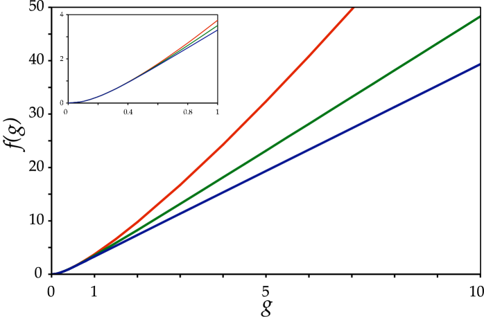
Figure 1: Plot of the solutions of the integral equations: $f_{m}(g)$ for the ES kernel $K^{(m)}$ (upper curve, red), $f_{0}(g)$ for the kernel $K^{(m)}+K^{(c)}$ (middle curve, green), and $f(g)$ for the BES kernel $K^{(m)}+2K^{(c)}$ (lower curve, blue). Notice the different asymptotic behaviors. The inset shows the three functions in the crossover region $0<g<1$.

We do not need to restrict the numerical analysis to real values of $g$; complex values of $g$ are of interest as well. In [19] it was argued that the dressing phase has singularities at $g\approx\pm in/4$, for $n=1,2,3,\ldots$. Also, their analysis of the small $g$ series shows that there are square root branch points in $f(g)$ at $g=\pm i/4$. Perhaps, this is related to the cuts in the giant-magnon dispersion relations [33, 34, 35, 36, 27], for momenta close to $\pi$. Our numerical results indeed indicate branch points at $g\approx\pm i/4,\pm i/2$ with exponent $1/2$. Beyond that we observe oscillations of both the real and imaginary parts of $f(g)$ for nearly imaginary $g$. Further work is needed to elucidate the analytical structure of $f(g)$.

3 Discussion

A very satisfying result of this paper is that the BES integral equation yields a smooth universal function $f(g)$ whose strong coupling expansion is in excellent numerical agreement with the spinning string predictions of [7, 9]. This provides a highly non-trivial confirmation of the AdS/CFT correspondence.

The agreement of this strong coupling expansion was anticipated in [19] based on a similar agreement of the dressing phase. However, some concerns about this argument were raised in [22] based on the slow convergence of the numerical extrapolations. Luckily, our numerical methods employed in solving the integral equation converge rapidly and produce a smooth function that approaches the asymptotics (2). The cross-over region of $f(g)$ where it changes from the perturbative to the linear behavior lies right around the radius of convergence, $g_{c}=1/4$, corresponding to $g_{YM}^{2}N=\pi^{2}$. For $N=3$, this would correspond to $\alpha_{s}\sim 0.25$.

The qualitative structure of the interpolating function $f(g)$ is quite similar to that involved in the circular Wilson loop, where the conjectured exact result [31, 32] is

$$\ln\left({I_{1}(4\pi g)\over 2\pi g}\right)\ .$$ (25)

The function (25) is analytic on the complex plane, with a series of branch cuts along the imaginary axis, and an essential singularity at infinity. The function $f(g)$ is also expected to have an infinite number of branch cuts along the imaginary axis, and an essential singularity at infinity [19].

Let us compare this with the exact anomalous dimension of a single giant magnon of momentum $p$ [33, 34, 35, 36, 27]:

$$-1+\sqrt{1+16g^{2}\sin^{2}\left(\frac{p}{2}\right)}\ .$$ (26)

This function has a single branch cut along the imaginary axis, going from $g=\frac{i}{4\sin\left(\frac{p}{2}\right)}$ to infinity, and no essential singularity at infinity. Observables of the gauge theory are composites of giant magnons with various momenta $p\in(0,2\pi)$. We thus expect the anomalous dimension of a generic unprotected operator to have a superposition of many cuts along the imaginary axis. This should endow a generic multi-magnon state with an analytic structure similar to that of $f(g)$.

We found numerically the presence, in $f(g)$, of the first two branch cuts on the imaginary axis, starting at $g=\pm\frac{ni}{4}$, $n=1,2$. The first of them, which also occurs for the giant magnon with maximal momentum $p=\pi$, agrees with the summation of the perturbative series [19]. The full structure of $f(g)$ is expected to contain an infinite number of branch cuts accumulating at infinity, where an essential singularity is present.

It is remarkable that the integral equation of [19] allows $f(g)$, which is not a BPS quantity, to be solved for. Hopefully, this paves the way to finding other observables as functions of the coupling in the planar ${\cal N}=4$ SYM theory.

References

- [1] D. J. Gross and F. Wilczek, “Asymptotically free gauge theories. 2,” Phys. Rev. D9 (1974) 980–993; H. Georgi and D. Politzer, “Electroproduction Scaling in an Asymptotically Free Theory of Strong Interactions,” Phys. Rev. D9 (1974) 416–420.
- [2] E.G. Floratos, D.A. Ross, Christopher T. Sachrajda, Nucl. Phys. B152 (1979) 493.
- [3] G. P. Korchemsky, “Asymptotics of the Altarelli-Parisi-Lipatov evolution kernels of parton distributions,” Mod. Phys. Lett. A 4, 1257 (1989). G. P. Korchemsky and G. Marchesini, “Structure function for large x and renormalization of Wilson loop,” Nucl. Phys. B 406, 225 (1993) [arXiv:hep-ph/9210281].
- [4] G. Sterman and M. E. Tejeda-Yeomans, “Multi-loop amplitudes and resummation,” Phys. Lett. B 552, 48 (2003) [arXiv:hep-ph/0210130].
- [5] A. V. Belitsky, A. S. Gorsky and G. P. Korchemsky, “Logarithmic scaling in gauge / string correspondence,” Nucl. Phys. B 748, 24 (2006) [arXiv:hep-th/0601112].
- [6] J. M. Maldacena, “The large limit of superconformal field theories and supergravity,” Adv. Theor. Math. Phys. 2, 231 (1998) [Int. J. Theor. Phys. 38, 1113 (1999)] [arXiv:hep-th/9711200]. S. S. Gubser, I. R. Klebanov and A. M. Polyakov, “Gauge theory correlators from non-critical string theory,” Phys. Lett. B 428, 105 (1998) [arXiv:hep-th/9802109]. E. Witten, “Anti-de Sitter space and holography,” Adv. Theor. Math. Phys. 2, 253 (1998) [arXiv:hep-th/9802150].
- [7] S. S. Gubser, I. R. Klebanov and A. M. Polyakov, “A semi-classical limit of the gauge/string correspondence,” Nucl. Phys. B 636, 99 (2002) [arXiv:hep-th/0204051].
- [8] M. Kruczenski, “A note on twist two operators in N = 4 SYM and Wilson loops in Minkowski signature,” JHEP 0212, 024 (2002) [arXiv:hep-th/0210115].
- [9] S. Frolov and A. A. Tseytlin, “Semiclassical quantization of rotating superstring in AdS(5) x S(5),” JHEP 0206, 007 (2002) [arXiv:hep-th/0204226].
- [10] A. V. Kotikov, L. N. Lipatov, A. I. Onishchenko and V. N. Velizhanin, “Three-loop universal anomalous dimension of the Wilson operators in N = 4 SUSY Yang-Mills model,” Phys. Lett. B 595, 521 (2004) [Erratum-ibid. B 632, 754 (2006)] [arXiv:hep-th/0404092].
- [11] Z. Bern, L. J. Dixon and V. A. Smirnov, “Iteration of planar amplitudes in maximally supersymmetric Yang-Mills theory at three loops and beyond,” Phys. Rev. D 72, 085001 (2005) [arXiv:hep-th/0505205].
- [12] S. Moch, J. A. M. Vermaseren and A. Vogt, “The three-loop splitting functions in QCD: The non-singlet case,” Nucl. Phys. B 688, 101 (2004) [arXiv:hep-ph/0403192].
- [13] L. N. Lipatov, “High-energy asymptotics of multicolor QCD and exactly solvable lattice models,” arXiv:hep-th/9311037.
- [14] L. D. Faddeev and G. P. Korchemsky, “High-energy QCD as a completely integrable model,” Phys. Lett. B 342, 311 (1995) [arXiv:hep-th/9404173].
- [15] V. M. Braun, S. E. Derkachov and A. N. Manashov, “Integrability of three-particle evolution equations in QCD,” Phys. Rev. Lett. 81, 2020 (1998) [arXiv:hep-ph/9805225].
- [16] J. A. Minahan and K. Zarembo, “The Bethe-ansatz for N = 4 super Yang-Mills,” JHEP 0303, 013 (2003) [arXiv:hep-th/0212208]. N. Beisert, C. Kristjansen and M. Staudacher, “The dilatation operator of N = 4 super Yang-Mills theory,” Nucl. Phys. B 664, 131 (2003) [arXiv:hep-th/0303060]. N. Beisert and M. Staudacher, “The N = 4 SYM integrable super spin chain,” Nucl. Phys. B 670, 439 (2003) [arXiv:hep-th/0307042].
- [17] For reviews, see N. Beisert, “The dilatation operator of N = 4 super Yang-Mills theory and integrability,” Phys. Rept. 405, 1 (2005) [arXiv:hep-th/0407277]; A. V. Belitsky, V. M. Braun, A. S. Gorsky and G. P. Korchemsky, “Integrability in QCD and beyond,” Int. J. Mod. Phys. A 19, 4715 (2004) [arXiv:hep-th/0407232].
- [18] D. Berenstein, J. M. Maldacena and H. Nastase, “Strings in flat space and pp waves from N = 4 super Yang Mills,” JHEP 0204, 013 (2002) [arXiv:hep-th/0202021].
- [19] N. Beisert, B. Eden and M. Staudacher, “Transcendentality and crossing,” arXiv:hep-th/0610251.
- [20] B. Eden and M. Staudacher, “Integrability and transcendentality,” arXiv:hep-th/0603157.
- [21] N. Beisert, R. Hernandez and E. Lopez, “A crossing-symmetric phase for AdS(5) x S**5 strings,” arXiv:hep-th/0609044.
- [22] Z. Bern, M. Czakon, L. J. Dixon, D. A. Kosower and V. A. Smirnov, “The four-loop planar amplitude and cusp anomalous dimension in maximally supersymmetric Yang-Mills theory,” arXiv:hep-th/0610248.
- [23] G. Arutyunov, S. Frolov and M. Staudacher, “Bethe ansatz for quantum strings,” JHEP 0410, 016 (2004) [arXiv:hep-th/0406256].
- [24] N. Beisert and T. Klose, “Long-range gl(n) integrable spin chains and plane-wave matrix theory,” J. Stat. Mech. 0607, P006 (2006) [arXiv:hep-th/0510124].
- [25] R. Hernandez and E. Lopez, “Quantum corrections to the string Bethe ansatz,” JHEP 0607, 004 (2006) [arXiv:hep-th/0603204].
- [26] L. Freyhult and C. Kristjansen, “A universality test of the quantum string Bethe ansatz,” Phys. Lett. B 638, 258 (2006) [arXiv:hep-th/0604069].
- [27] D. M. Hofman and J. M. Maldacena, “Giant magnons,” J. Phys. A 39, 13095 (2006) [arXiv:hep-th/0604135].
- [28] R. A. Janik, “The AdS(5) x S**5 superstring worldsheet S-matrix and crossing symmetry,” Phys. Rev. D 73, 086006 (2006) [arXiv:hep-th/0603038].
- [29] G. ’t Hooft, “Large N,” arXiv:hep-th/0204069.
- [30] A. V. Belitsky, “Long-range SL(2) Baxter equation in N = 4 super-Yang-Mills theory,” arXiv:hep-th/0609068.
- [31] J. K. Erickson, G. W. Semenoff, and K. Zarembo, “Wilson loops in N = 4 supersymmetric Yang-Mills theory,” Nucl. Phys. B582 (2000) 155–175, hep-th/0003055.
- [32] N. Drukker and D. J. Gross, “An exact prediction of N = 4 SUSYM theory for string theory,” J. Math. Phys. 42 (2001) 2896–2914, hep-th/0010274.
- [33] N. Beisert, “The su(22) dynamic S-matrix,” arXiv:hep-th/0511082.
- [34] N. Beisert, V. Dippel and M. Staudacher, “A novel long range spin chain and planar N = 4 super Yang-Mills,” JHEP 0407, 075 (2004) [arXiv:hep-th/0405001].
- [35] D. Berenstein, D. H. Correa and S. E. Vazquez, “All loop BMN state energies from matrices,” JHEP 0602, 048 (2006) [arXiv:hep-th/0509015].
- [36] A. Santambrogio and D. Zanon, “Exact anomalous dimensions of N = 4 Yang-Mills operators with large R charge,” Phys. Lett. B 545, 425 (2002) [arXiv:hep-th/0206079].