An Electroweak Oscillon

Abstract

A recent study demonstrated the existence of oscillons — extremely long-lived localized configurations that undergo regular oscillations in time — in spontaneously broken $SU(2)$ gauge theory with a fundamental Higgs particle whose mass is twice the mass of the gauge bosons. This analysis was carried out in a spherically symmetric ansatz invariant under combined spatial and isospin rotations. We extend this result by considering a numerical simulation of the the full bosonic sector of the $SU(2)\times U(1)$ electroweak Standard Model in $3+1$ dimensions, with no assumption of rotational symmetry, for a Higgs mass equal to twice the $W^{\pm}$ boson mass. Within the limits of this numerical simulation, we find that the oscillon solution from the pure $SU(2)$ theory is modified but remains stable in the full electroweak theory. The observed oscillon solution contains total energy approximately 30 TeV localized in a region of radius approximately 0.05 fm.

Introduction

In nonlinear field theories, static soliton solutions to the equations of motion have been well studied (see for example Coleman ; Rajaraman ). However, a much broader class of theories contain oscillon solutions, which are localized in space but oscillate in time. In some special cases, such as the sine-Gordon breather DHN and $Q$-ball ColemanQ , conserved charges guarantee the existence of exact, periodic solutions. Even in the absence of such guarantees, however, localized solutions have been found in many different theories that either live indefinitely or for extremely long times compared to the natural timescales of the system.

For scalar theories in one space dimension, oscillon solutions have been found to remain periodic to all orders in a perturbative expansion DHN and are never seen to decay in numerical simulations Campbell , but can decay after extremely long times via nonperturbative effects Kruskal or by coupling to an expanding background oscex . Both $\phi^{4}$ theory in two dimensions 2d1 ; 2d2 and the abelian Higgs model in one dimension abelianhiggs have also been shown to contain oscillon solutions that are not observed to decay. In $\phi^{4}$ theory in three dimensions Bogolyubsky ; Gleiser ; Honda ; iball ; Forgacs , however, there exist long-lived quasi-periodic solutions whose lifetime depends sensitively on the initial conditions. Similar behavior is present in other scalar theories in three dimensions Wojtek and in higher dimensions Gleiserd . Phenomenologically, small $Q$-balls were considered as dark matter candidates in smallq1 ; smallq2 ; Enqvist ; Kasuya , axion oscillons were considered in Kolb , and the possible role of oscillons in and after inflation was studied in McDonald ; Rajantie ; Gleiserinflat . Oscillon-like solutions have also been studied in connection with phase transitions Gleiserphase , monopole systems monopole , QCD Hsu , and gravitational systems Khlopov .

A recent paper oscillon demonstrated numerical evidence for an oscillon solution in spontaneously broken $SU(2)$ gauge theory with a fundamental Higgs whose mass is exactly twice that of the gauge bosons. Current work twofield is investigating an analytic explanation of this mass relationship using a small amplitude analysis DHN ; Hsu ; smallamp , in which the $2:1$ ratio arises as a resonance condition necessary for quadratic nonlinear terms to balance dispersive linear terms in the equations of motion. In this analysis, a field of mass $m$ oscillates with amplitude $\epsilon m$, frequency $m\sqrt{1-\epsilon^{2}}$, and length scale $1/(\epsilon m)$. A similar mass relation arises in the study of embedded defects Lepora . The field configurations in oscillon were restricted to the spherical ansatz spherical , meaning they were invariant under combined rotations in space and isospin. Here we extend this analysis to a fully three-dimensional spatial lattice, eliminating any symmetry assumptions. We include the $U(1)$ hypercharge field, so that we are simulating the full electroweak sector of the Standard Model without fermions. We use the same $SU(2)$ gauge coupling $g$ and Higgs self-coupling $\lambda$ as in the pure $SU(2)$ theory, meaning that the Higgs mass is twice the mass of the $W^{\pm}$ bosons, and set the $U(1)$ coupling $g^{\prime}$ so that the mass of the $Z^{0}$ boson matches its observed value.

While one might expect the oscillon to decay rapidly by emitting electromagnetic radiation, it does not. Instead, after initially shedding some energy into electromagnetic radiation, the system settles into a stable, localized oscillon solution that no longer radiates. Similar behavior was observed both when an additional massless scalar field was coupled to breathers in one-dimensional $\phi^{4}$ theory and when an additional spherically symmetric massless scalar field was coupled to oscillons in the spherical ansatz, results that provided motivation for this work.

Continuum Theory

We begin from $SU(2)\times U(1)$ electroweak theory in the continuum, ignoring fermions. We follow the standard classical treatment of spontaneously broken nonabelian field theory (see for example Huang ). The Lagrangian density is

$${\cal L}=(D_{\mu}\Phi)^{\dagger}D^{\mu}\Phi-\frac{1}{4}F_{\mu\nu}F^{\mu\nu}-\frac{1}{4}{\bm{F}}_{\mu\nu}\cdot{\bm{F}}^{\mu\nu}-\lambda(|\Phi|^{2}-v^{2})^{2}\,,$$ (1)

where the boldface vector notation refers to isovectors. Here $\Phi$ is the Higgs field, a Lorentz scalar carrying $U(1)$ hypercharge $1/2$ and transforming under the fundamental representation of $SU(2)$. The metric signature is $+---$. The $SU(2)$ and $U(1)$ field strengths are

$$\bm{F}_{\mu\nu} = \partial_{\mu}{\bm{W}}_{\nu}-\partial_{\nu}\bm{W}_{\mu}-g{\bm{W}}_{\mu}\times{\bm{W}}_{\nu}\,,$$ (2)

$$F_{\mu\nu} = \partial_{\mu}B_{\nu}-\partial_{\nu}B_{\mu}\,,$$ (3)

and the covariant derivatives are given by

$$D_{\mu}\Phi = \left(\partial_{\mu}+i\frac{g^{\prime}}{2}B_{\mu}+i\frac{g}{2}\bm{\tau}\cdot\bm{W}_{\mu}\right)\Phi\,,$$ (4)

$$D^{\mu}\bm{F}_{\mu\nu} = \partial^{\mu}\bm{F}_{\mu\nu}-g\bm{W}^{\mu}\times\bm{F}_{\mu\nu}\,,$$ (5)

where $\bm{\tau}$ represents the weak isospin Pauli matrices. We obtain the equations of motion

$$\partial_{\mu}F^{\mu\nu} = J^{\nu}\,,$$ (6)

$$D_{\mu}\bm{F}^{\mu\nu} = \bm{J}^{\nu}\,,$$ (7)

$$D^{\mu}D_{\mu}\Phi = 2\lambda(v^{2}-|\Phi|^{2})\Phi\,,$$ (8)

where the gauge currents are

$$J_{\nu} = g^{\prime}{\,\rm Im\,}(D_{\nu}\Phi)^{\dagger}\Phi\,,$$ (9)

$$\bm{J}_{\nu} = g{\,\rm Im\,}(D_{\nu}\Phi)^{\dagger}\bm{\tau}\Phi\,.$$ (10)

We work in the gauge $B_{0}=0$, $\bm{W}_{0}=\bm{0}$. With this choice, the covariant time derivatives become ordinary derivatives and we can apply a Hamiltonian formalism. The energy density is

$$u = \frac{1}{2}\sum_{j=x,y,z}\Bigg{[}\dot{B}_{j}^{2}+\bm{\dot{W}}_{j}\cdot\bm{\dot{W}}_{j}+\sum_{k>j}\left(F_{kj}^{2}+\bm{F}_{kj}\cdot\bm{F}_{kj}\right)\Bigg{]}$$ (11)

$$+ |\dot{\Phi}|^{2}+\sum_{j=x,y,z}(D_{j}\Phi)^{\dagger}(D_{j}\Phi)+\lambda\left(|\Phi|^{2}-v^{2}\right)^{2}\,,$$ (12)

whose integral over space is conserved. Here dot indicates time derivative. From the equations for $B_{0}$ and $\bm{W}_{0}$, we obtain the Gauss’s Law constraints,

$$\sum_{j=x,y,z}\partial_{j}\dot{B}_{j}-J_{0} =0\,,$$ (13)

$$\sum_{j=x,y,z}D_{j}\bm{\dot{W}}_{j}-\bm{J}_{0} = 0\,,$$ (14)

where the charge densities are

$$J_{0} = g^{\prime}{\,\rm Im\,}\dot{\Phi}^{\dagger}\Phi\,,$$ (15)

$$\bm{J}_{0} = g{\,\rm Im\,}\dot{\Phi}^{\dagger}\bm{\tau}\Phi\,.$$ (16)

These constraints remain true at all times, at all points in space, assuming they are obeyed by the initial value data.

Lattice Theory

We use the standard Wilsonian approach Wilson for implementing gauge fields on the lattice (for a review see SmitBook ), adapted to Minkowski space evolution as in Shaposhnikov ; SmitSim ; RajantieSim . (The details of the discretization have been modified slightly for the present application.) The $U(1)$ and $SU(2)$ gauge fields live on the links of the lattice and the fundamental Higgs field lives at the lattice sites. The lattice spacing is $\Delta x$, and we determine the values of the fields at time $t_{+}=t+\Delta t$ based on their values at times $t$ and $t_{-}=t-\Delta t$. We associate with the link emanating from lattice site $p$ in the positive $j^{\rm th}$ direction the Wilson line

$$U_{j}^{p}=e^{ig^{\prime}B_{j}^{p}\Delta x/2}e^{ig\bm{W}_{j}^{p}\cdot\bm{\tau}\Delta x/2}\,.$$ (17)

We define the Wilson line for the link emanating from lattice site $p$ in the negative $j^{\rm th}$ direction to be the adjoint of the corresponding Wilson line emanating in the positive direction from the neighboring site, $U_{-j}^{p}=(U_{j}^{p-j})^{\dagger}$, where the notation $p\pm j$ indicates the adjacent lattice site to $p$, displaced from $p$ in direction $\pm j$. At the edges of the lattice we use periodic boundary conditions. We define the logarithm of $2\times 2$ matrices of this form as

$$\ln U_{j}^{p}=\frac{i\Delta x}{2}(g^{\prime}B_{j}^{p}+g\bm{W}_{j}^{p}\cdot\bm{\tau})\,,$$ (18)

and note that $\ln AB\neq\ln A+\ln B$ when the matrices do not commute.

The equation of motion for the Higgs field at site $p$ is

$$\Phi^{p}(t_{+})=2\Phi^{p}-\Phi^{p}(t_{-})+\Delta t^{2}\ddot{\Phi}^{p}\,,$$ (19)

where

$$\ddot{\Phi}^{p}=\sum_{j=\pm x,\pm y,\pm z}\frac{U_{j}^{p}\Phi^{p+j}-\Phi^{p}}{\Delta x^{2}}+2\lambda\left(v^{2}-|\Phi^{p}|^{2}\right)\Phi^{p}\,,$$ (20)

and all fields are evaluated at time $t$ unless otherwise indicated. For the gauge fields, we have

$$U_{j}^{p}(t_{+})=\exp\Bigg{[}\ln U_{j}^{p}U_{j}^{p}(t_{-})^{\dagger}+\Bigg{(}\frac{\Delta x}{2i}(g^{\prime}J_{j}^{p}+g\bm{J}_{j}^{p}\cdot\bm{\tau})$$ (21)

$$-\sum_{j^{\prime}\neq j}\frac{\ln U^{p}_{\square(j,j^{\prime})}+\ln U^{p}_{\square(j,-j^{\prime})}}{\Delta x^{2}}\Bigg{)}\Delta t^{2}\Bigg{]}U_{j}^{p}\,,~{}~{}~{}$$ (22)

where $U^{p}_{\square(j,j^{\prime})}=U_{j}^{p}U_{j^{\prime}}^{p+j}U_{-j}^{p+j+j^{\prime}}U_{-j^{\prime}}^{p+j^{\prime}}$ and

$$J_{j}^{p} = g^{\prime}{\rm\,Im\,}\frac{(\Phi^{p})^{\dagger}U_{j}^{p}\Phi^{p+j}}{\Delta x}\,,$$ (23)

$$\bm{J}_{j}^{p} = g{\rm\,Im\,}\frac{(\Phi^{p})^{\dagger}\bm{\tau}U_{j}^{p}\Phi^{p+j}}{\Delta x}\,,$$ (24)

are the gauge currents. The energy density at $p$ is then

$$u^{p} = \sum_{j=x,y,z}\Bigg{[}\frac{1}{2}\frac{\left\|\exp\left(\ln U_{j}^{p}(t_{+})-\ln U_{j}^{p}(t_{-})\right)\right\|^{2}}{(2\Delta t)^{2}}$$ (25)

$$+ \frac{1}{2}\sum_{j^{\prime}>j}\frac{\left\|U^{p}_{\square(j,j^{\prime})}\right\|^{2}}{\Delta x^{2}}+\frac{\left|U_{j}^{p}\Phi^{p+j}-\Phi^{p}\right|^{2}}{\Delta x^{2}}\Bigg{]}$$ (26)

$$+ \frac{\left|\Phi^{p}(t_{+})-\Phi^{p}(t_{-})\right|^{2}}{4\Delta t^{2}}+\lambda\left(|\Phi^{p}|^{2}-v^{2}\right)^{2}\,,$$ (27)

whose integral over the whole lattice is conserved. Here we have defined

$$\left\|U_{j}^{p}\right\|^{2} = \frac{\left|{\rm Tr\,}\ln U_{j}^{p}\right|^{2}}{g^{\prime 2}\Delta x^{2}}+\frac{\left({\rm Tr\,}\bm{\tau}\ln U_{j}^{p}\right)^{\dagger}\cdot\left({\rm Tr\,}\bm{\tau}\ln U_{j}^{p}\right)}{g^{2}\Delta x^{2}}$$ (28)

$$= |B_{j}^{p}|^{2}+\bm{W}_{j}^{p}\cdot\bm{W}_{j}^{p}$$ (29)

for any $U(2)$ link matrix.

At every lattice point, Gauss’s Law,

$$\sum_{j=x,y,z}\frac{\ln U_{j}^{p}(t_{+})U_{j}^{p}(t_{-})^{\dagger}+\ln U_{-j}^{p}(t_{+})U_{-j}^{p}(t_{-})^{\dagger}}{i\Delta x^{2}\Delta t}$$ (30)

$$-\left(g^{\prime}J_{0}^{p}+g\bm{J}_{0}^{p}\cdot\bm{\tau}\right)=0\,,$$ (31)

is also maintained throughout the evolution, where the charge densities are given by

$$J_{0} = g^{\prime}{\rm\,Im\,}\left(\frac{\Phi^{p}(t_{+})-\Phi^{p}(t_{-})}{2\Delta t}\right)^{\dagger}\Phi^{p}\,,$$ (32)

$$\bm{J}_{0} = g{\rm\,Im\,}\left(\frac{\Phi^{p}(t_{+})-\Phi^{p}(t_{-})}{2\Delta t}\right)^{\dagger}\bm{\tau}\Phi^{p}\,.$$ (33)

Numerical Simulation

The initial conditions for the simulation are obtained starting from an approximate functional fit to the oscillon solutions found in numerical simulations of the $SU(2)$-Higgs theory in the spherical ansatz oscillon . This result provides the initial data for the $\bm{W}$ and $\Phi$ fields, and the initial $B$ field is chosen to vanish. In order to guarantee that the initial configuration continues to obey Gauss’s Law in the full $SU(2)\times U(1)$ theory, we generate the fit at a point in the cycle where the time derivatives are smallest, and impose the requirement that all time derivatives vanish for our initial data.

The initial conditions are of the spherical ansatz form

$$\bm{\tau}\cdot\bm{W}_{i} = \frac{1}{g}\left[a_{1}(r,t)\bm{\tau}\cdot\bm{\hat{x}}\hat{x}_{i}+\frac{\alpha(r,t)}{r}(\tau_{i}-{\bm{\tau}}\cdot\bm{\hat{x}}\hat{x}_{i})\right.$$ (37)

$$\left.-\frac{\gamma(r,t)}{r}(\bm{\hat{x}}\times\bm{\tau})_{i}\right],$$

$$\Phi = \frac{1}{g}\left[\mu(r,t)-i\nu(r,t)\,{\bm{\tau}}\cdot\bm{\hat{x}}\right]\pmatrix{0\cr 1}\,,$$ (38)

where $\bm{\hat{x}}=\bm{x}/r$ and $r$ is the distance from the origin. The field definitions have been chosen so that the reduced fields match those used in oscillon , even though the conventions for the three-dimensional theory used here are slightly different. We work in units where $v=1/\sqrt{2}$. Since we are dealing with classical dynamics, we can rescale the fields to fix the $SU(2)$ coupling constant at $g=\sqrt{2}$, so that the $W^{\pm}$ mass is then $m_{W}=gv/\sqrt{2}=1/\sqrt{2}$. With this rescaling, we must also introduce an overall factor of $g^{2}/g_{W}^{2}$ multiplying the total energy, where $g_{W}=0.634$ is the true weak coupling constant. We choose $\lambda=1$, so that the Higgs mass is twice the $W^{\pm}$ mass, $m_{H}=2v\sqrt{\lambda}=\sqrt{2}$. These choices of units and normalization agree with oscillon , except the quantity called $v$ here is smaller than $v$ in oscillon by a factor of $\sqrt{2}$. Finally, we fix $g^{\prime}=0.773$, so that the ratio $g^{\prime}/g$ matches the observed value and the $Z^{0}$ boson has the correct mass.

In these units, we consider initial configurations

$$a_{1}(r) = \epsilon(0.117\epsilon+0.016\epsilon r)\left({\,\rm sech\,}2\epsilon r\right)^{1/8}\,,$$ (39)

$$\mu(r) = 1-0.138\epsilon{\,\rm sech\,}\frac{\epsilon r}{6.75}\,,$$ (40)

$$\nu(r) = 0.017\epsilon r{\,\rm sech\,}\frac{\epsilon r}{5}\,,$$ (41)

$$\alpha(r) = 0.117\epsilon^{2}r{\,\rm sech\,}\frac{\epsilon r}{8}\,,$$ (42)

$$\gamma(r) = 0\,,$$ (43)

where the adjustable parameter $\epsilon$ allows us to include a combined rescaling of the fields’ amplitudes and $r$-dependence, as is commonly used in a small amplitude analysis DHN ; Hsu ; smallamp . While $\epsilon=1$ gives an approximation to the spherical ansatz solution of oscillon , a slightly larger value appears to be necessary for the configuration to settle into a stable solution in the full $SU(2)\times U(1)$ model. The first term in parentheses in the definition of $a_{1}(r)$ is scaled with an additional $\epsilon$ so that it matches the coefficient of $\alpha$, ensuring that $\alpha$, $a_{1}-\alpha/r$, $\gamma/r$, and $\nu$ all vanish as $r\to 0$, as required for regularity of the fields at the origin. Within the spherical ansatz simulation, these initial conditions settle into a long-lived oscillon in the pure $SU(2)$-Higgs theory, which we never see decay. The $U(1)$ interactions break the grand spin symmetry of the spherical ansatz, though the continuum theory still preserves invariance under combined space and isospin rotations around the $z$-axis. The Cartesian lattice provides a small breaking of all rotational symmetries. Thus configurations at later times are not constrained to lie within this reduced ansatz. (The full three-dimensional simulation does continue to agree with the spherical ansatz simulation for the case when the $U(1)$ interaction is turned off, another check of the numerical calculation.)

We start from these initial conditions and let the system evolve for as long as is practical numerically. One concern is that the outgoing radiation emitted as the configuration settles into the oscillon solution can wrap around the periodic boundary conditions, return to the region of the oscillon, and potentially destabilize it. However, as long as the region in which the oscillon is localized does not represent a significant fraction of the lattice volume, this radiation is sufficiently diffuse that it does not affect the oscillon. We use a lattice of size $L=144$ on a side in natural units, which is more than enough to satisfy this criterion. For $L\gtrsim 100$, changing the lattice size simply changes the pattern of noise caused by electromagnetic radiation superimposed on the oscillon region, but does not affect oscillon properties or stability. We can therefore be certain that there is no coherent structure to this unphysical radiation that could possibly be necessary for the oscillon’s stability; its only possible effect is to destabilize the oscillon, which only occurs if the radiation is artificially concentrated by a small lattice (e.g. of size $L<100$). In numerical experiments, these destabilization effects are actually much weaker in the electroweak model than in pure scalar or $SU(2)$ Higgs-gauge models, because in the electroweak model the radiated energy is almost entirely in the electromagnetic field, while the oscillon solution arranges itself to be electrically neutral. For this reason, it is not necessary to use absorptive techniques such as adiabatic damping 2d1 (which would have to be adapted to accommodate gauge invariance) or an expanding background oscex .

We use lattice spacing $\Delta x=0.75$, though $\Delta x=0.625$ and $\Delta x=0.25$ were verified to give completely equivalent results in smaller tests. The time step is $\Delta t=0.1$. Total energy is conserved to a few parts in $10^{3}$, which is appropriate since our algorithm is second-order accurate. To check Gauss’s Law, we square the left-hand side of Eq. (31), take the trace, and then take the square root of the result. The integral of this quantity over the lattice never exceeds $0.025$ and shows no upward trend over time, a highly nontrivial check on the numerical calculation. It is necessary, however, to use double precision to avoid very gradual degradation in this result. A run to time $10,000$ takes roughly $40$ hours using $24$ parallel processes, each running on a $2\ {\rm GHz}$ Opteron processor core.

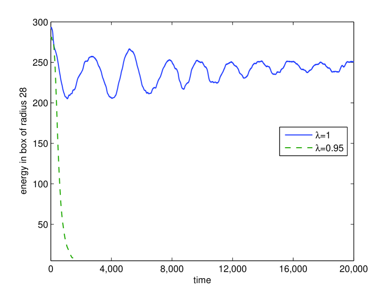
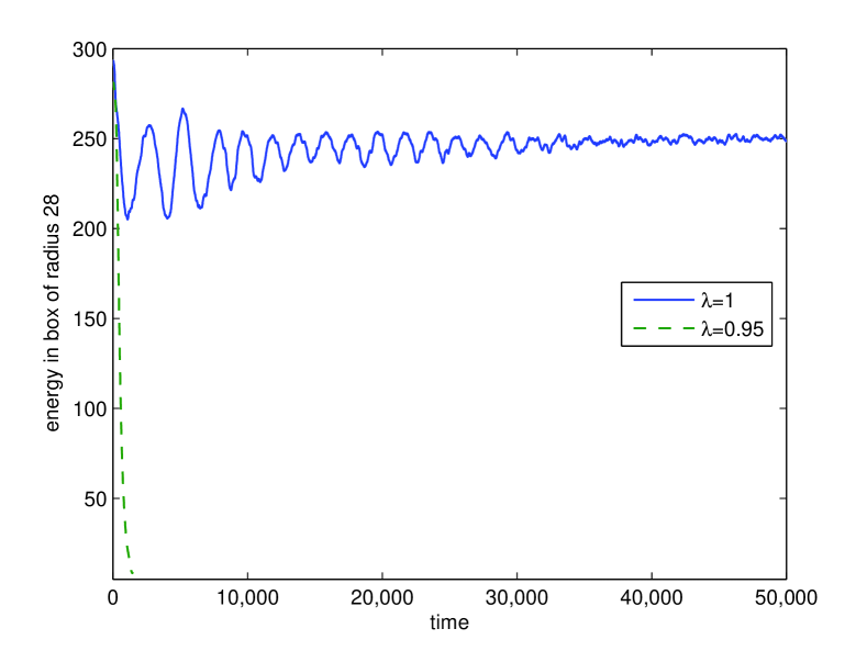
Figure 1: Energy in a box of radius 28 as a function of time in the natural units of oscillon . One unit of energy is $114\ {\rm GeV}$, one unit of time is $5.79\times 10^{-27}\ {\rm sec}$, and one unit of length is $1.74\times 10^{-18}\ {\rm m}$. In the top panel, the initial conditions are given by Eq. (43) with $\epsilon=1.15$. In the bottom panel, the initial conditions are the same except the $\tau_{z}$ component of $\bm{W}$ in Eq. (38) has been set to zero. Two values of the Higgs self-coupling $\lambda$ are shown. For $\lambda=1$, the masses of the Higgs and $W$ fields are in the $2:1$ ratio needed for oscillon formation and the solution remains localized throughout the simulation. A transient beat pattern is also visible. For $\lambda=0.95$, the mass ratio is $1.95:1$. In that case, there is no stable object and the solution quickly disperses.

Figure 1 shows the energy in a spherical box of radius $28$ as the fields are evolved from the initial conditions in Eq. (43). When the Higgs mass is twice the $W^{\pm}$ mass, only a small amount of energy is emitted from the central region, with the rest remaining localized for the length of the simulation in a stable oscillon solution. If the masses are not in this ratio, however, the initial configuration quickly disperses. The box radius has been chosen to be just large enough to enclose essentially all of energy density associated with the stable oscillon solution. As a result, as the initial conditions settle into the stable oscillon solution, we are also able to see a transient “beat” pattern: the field configurations gradually expand and contract slightly over many periods, causing a small amount of energy to move in and out of the box, accompanied by a corresponding modulation of the field amplitudes. (When a larger box size is used, the graph of the energy in the box flattens out.) Similar beats appear in the $SU(2)$ spherical ansatz oscillon oscillon , but in the electroweak oscillon their amplitude decays more rapidly. As in the spherical ansatz oscillon, in the electroweak oscillon each excited field oscillates at a frequency just below its mass, with amplitude of order $0.1$ and typical radius of order $10$ in our units. By comparing the total number of cycles to the total time, we find $\omega_{H}=1.404$ for the Higgs field components and $\omega_{W}=0.702$ for the gauge field components. The primary excitations are in the $W^{\pm}$ fields and the $\Phi$ field, with some energy radiated outward in the electromagnetic field in a dipole pattern and the $Z^{0}$ field largely absent. In contrast, in the spherical ansatz oscillon the $W^{\pm}$ and $Z^{0}$ fields must appear symmetrically. The electroweak oscillon does remain approximately axially symmetric under combined space and isospin rotations around the $z$-axis. These results suggest a simple modification of the initial configurations in which the $\tau_{z}$ component of $\bm{W}$ is set to zero in Eq. (38). This modification yields an equivalent final oscillon configuration, with the same field amplitudes, localized energy and field frequencies. However, less energy is shed initially, so there is less superimposed noise caused by radiation returning from the boundaries. As a result, the beat pattern is also more clearly visible. This case is also shown in Fig. 1.

Conclusions

We have seen strong evidence for the existence of a long-lived, localized, oscillatory solution to the field equations of the bosonic electroweak sector of the Standard Model in the case where the Higgs mass is twice the $W^{\pm}$ mass. Compared to the natural scales of the system, this solution has fairly small field amplitudes, but because of its large spatial extent it is very massive. Such large, coherent objects are well described by the classical analysis undertaken here. Quantization of the small oscillations around the oscillon solution would nonetheless be of interest, perhaps using methods similar to those applied to $Q$-ball oscillons in qqball .

Forming oscillons would likely require large energies available only in the early universe. In this context, it would be very desirable to incorporate fermion couplings, which have been ignored here. (Of course, lattice chiral fermions introduce significant, but not insurmountable, technical complications.) While one might expect the oscillon to be destabilized by decay to light fermions, in the case of the photon coupling we have seen that the analogous decay mechanism is highly suppressed. A slow fermion decay mode would be of particular interest in baryogenesis, since it would provide a mechanism for fermions to be produced out of equilibrium, as is necessary to avoid washout of particle/antiparticle asymmetry. Or, if the oscillon is extremely long-lived, it could provide a dark matter candidate. If such results proved compelling, this analysis would suggest a preferred value of the Higgs mass.

References

- (1) S. Coleman, Aspects of Symmetry (Cambridge University Press, 1985).
- (2) R. Rajaraman, Solitons and Instantons (North-Holland, 1982).
- (3) R. F. Dashen, B. Hasslacher and A. Neveu, Phys. Rev. D11 (1975) 3424.
- (4) S. Coleman, Nucl. Phys. B262 (1985) 263.
- (5) D. K. Campbell, J. F. Schonfeld and C. A. Wingate, Physica 9D (1983) 1.
- (6) H. Segur and M. D. Kruskal, Phys. Rev. Lett. 58 (1987) 747.
- (7) N. Graham and N. Stamatopoulos, hep-th/0604134, Phys. Lett. B639 (2006) 541.
- (8) M. Gleiser and A. Sornborger, patt-sol/9909002, Phys. Rev. E62 (2000) 1368.
- (9) M. Hindmarsh and P. Salmi, hep-th/0606016.
- (10) C. Rebbi and R. Singleton, Jr., hep-ph/9601260, Phys. Rev. D54 (1996) 1020; P. Arnold and L. McLerran, Phys. Rev. D37 (1988) 1020.
- (11) I. L. Bogolyubsky and V. G. Makhankov, JETP Lett. 24 (1976) 12.
- (12) M. Gleiser, hep-ph/9308279, Phys. Rev. D49 (1994) 2978; E. J. Copeland, M. Gleiser and H. R. Muller, hep-ph/9503217, Phys. Rev. D52 (1995) 1920; A. Adib, M. Gleiser and C. Almeida, hep-th/0203072, Phys. Rev. D66 (2002) 085011.
- (13) E. P. Honda and M. W. Choptuik, hep-ph/0110065, Phys. Rev. D65 (2002) 084037.
- (14) S. Kasuya, M. Kawasaki and F. Takahashi, hep-ph/ 0209358, Phys. Lett. B559 (2003) 99.
- (15) G. Fodor, P. Forgács, P. Grandclément and I. Rácz, hep-th/0609023.
- (16) B. Piette and W. J. Zakrzewski, Nonlin. 11 (1998) 1103.
- (17) M. Gleiser, hep-th/0408221, Phys. Lett. B600 (2004) 126; P. M. Saffin and A. Tranberg, hep-th/0610191.
- (18) A. Kusenko, hep-th/9704073, Phys. Lett. B404 (1997) 285.
- (19) A. Kusenko and M. E. Shaposhnikov, hep-ph/9709492, Phys. Lett. B418 (1998) 46.
- (20) K. Enqvist and J. McDonald, hep-ph/9711514, Phys. Lett. B425 (1998) 309.
- (21) S. Kasuya and M. Kawasaki, hep-ph/9909509, Phys. Rev. D61 (2000) 041301.
- (22) E. W. Kolb and I. Tkachev, astro-ph/9311037, Phys. Rev. D49 (1994) 5040.
- (23) M. Broadhead and J. McDonald, hep-ph/0503081, Phys. Rev. D72 (2005) 043519.
- (24) A. Rajantie and E. J. Copeland, hep-ph/0003025, Phys. Rev. Lett. 85 (2000) 916;
- (25) M. Gleiser, hep-th/0602187.
- (26) M. Gleiser and R. C. Howell, hep-ph/0209176, Phys. Rev. E68 (2003) 065203(R); hep-ph/0409179, Phys. Rev. Lett. 94 (2005) 151601.
- (27) G. Fodor and I. Rácz, hep-th/0311061, Phys. Rev. Lett. 92 (2004) 151801; P. Forgács and M. S. Volkov, hep-th/0311062, Phys. Rev. Lett. 92 (2004) 151802; G. Fodor and I. Rácz, hep-th/0609110.
- (28) J. N. Hormuzdiar and S. D. Hsu, hep-ph/9805382, Phys. Rev. C59 (1999) 889.
- (29) I. Dymnikova, M. Yu. Khlopov, L. Koziel and S. G. Rubin, hep-th/0010120, Grav. Cosm. 6 (2000) 311.
- (30) E. Farhi, N. Graham, V. Khemani, R. Markov and R. R. Rosales, hep-th/0505273, Phys. Rev. D72 (2005) 101701.
- (31) E. Farhi, N. Graham, A. Guth, R. R. Rosales and R. Stowell, in progress.
- (32) A. M. Kosevich and A. S. Kovalev, Zh. Eksp. Teor. Fiz. 67 (1975) 1793; R. R. Rosales, private communication.
- (33) N. F. Lepora, hep-th/0210018, Phys. Lett. B541 (2002) 362.
- (34) R. F. Dashen, B. Hasslacher and A. Neveu, Phys. Rev. D10 (1974) 4138; E. Witten, Phys. Rev. Lett. 38 (1977) 121; P. Forgács and N. S. Manton, Commun. Math. Phys. 72 (1980) 15; B. Ratra and L. G. Yaffe, Phys. Lett. B205 (1988) 57.
- (35) K. Huang, Quarks, Leptons and Gauge Fields (World Scientific, 1992).
- (36) K. Wilson, Phys. Rev. D10 (1974) 2445.
- (37) J. Smit, Introduction to Quantum Fields on a Lattice, (Cambridge University Press, 2001).
- (38) J. Ambjorn, T. Askgaard, H. Porter and M. E. Shaposhnikov, Nucl. Phys. B353 (1991) 346.
- (39) A. Tranberg and J. Smit, hep-ph/0310342, JHEP 0311 (2003) 016.
- (40) A. Rajantie, P. M. Saffin and E. J. Copeland, hep-ph/0012097, Phys. Rev. D 63 (2001) 123512.
- (41) N. Graham, hep-th/0105009, Phys. Lett. B513 (2001) 112.