Zonotopes and four-dimensional superconformal field theories

Abstract:

The $a$-maximization technique proposed by Intriligator and Wecht allows us to determine the exact $R$-charges and scaling dimensions of the chiral operators of four-dimensional superconformal field theories. The problem of existence and uniqueness of the solution, however, has not been addressed in general setting. In this paper, it is shown that the $a$-function always has a unique critical point which is also a global maximum for a large class of quiver gauge theories specified by toric diagrams. Our proof is based on the observation that the $a$-function is given by the volume of a three dimensional polytope called “zonotope”, and the uniqueness essentially follows from Brunn-Minkowski inequality for the volume of convex bodies. We also show a universal upper bound for the exact $R$-charges, and the monotonicity of $a$-function in the sense that $a$-function decreases whenever the toric diagram shrinks. The relationship between $a$-maximization and volume-minimization is also discussed.

1 Introduction

One of the most important problems in quantum field theories is to understand the renormalization group (RG) flows and the universality classes.

In two dimensions, we have a fairly satisfactory global picture of the moduli space $\mathcal{M}_{\mathrm{2dQFT}}$ of quantum field theories. Zamolodchikov [1] introduced a real valued function $c:\mathcal{M}_{\mathrm{2dQFT}}\to{\mathbb{R}}$ and showed that the RG flow is a gradient flow of $c$ with respect to the metric defined by two-point correlation functions. In particular, $c$ is monotonically decreasing along the RG flow. Each critical point of $c$ corresponds to a fixed point of the RG flow i.e. a conformal field theory, and the critical value is the central charge of the Virasoro algebra of the corresponding conformal field theory.

Considerable effort has been expended to generalize these ideas to to four dimensions. As the Zamolodchikov’s $c$-function is related the trace anomaly of the stress energy tensor, natural candidates for four dimensional theories are the coefficients $a$ and $c$ of trace anomaly [2]

$$g_{ij}\left\langle T^{ij}\right\rangle=-aE_{4}-cI_{4}$$

where

$$E_{4} = \frac{1}{16\pi^{2}}\bigl{(}R^{ijkl}R_{ijkl}-4R^{ij}R_{ij}+R^{2}\bigr{)},$$

$$I_{4} = -\frac{1}{16\pi^{2}}\bigl{(}R^{ijkl}R_{ijkl}-2R^{ij}R_{ij}+\frac{1}{3}R^{2}\bigr{)},$$

where $R_{ijkl}$ denotes the Riemann curvature of the background geometry. It is now believed [3] that $a$-function will play a similar role to Zamolodchikov’s $c$ function: $a$ decreases along any RG flow.

It is usually difficult to compute $a$-functions. The situation is much better if the field theories has supersymmetry. Any four dimensional superconformal fields theory (SCFT) has global symmetry supergroup $SU(2,2|1)$; $SO(4,2)\times U(1)_{R}$ is its bosonic subgroup. For the representation of the superconformal algebra on the chiral supermultiplet [4, 5], there is a simple relation between the $R$-charge and the conformal dimension $\Delta$ of a operator $\mathcal{O}$

$$\Delta(\mathcal{O})=\frac{3}{2}R(\mathcal{O}).$$

The scaling dimensions of chiral operators are protected from quantum corrections. Anselmi et al. [6, 7] have shown that the $U(1)_{R}$ ’t Hooft anomalies completely determine the $a$ and $c$ central charges of the superconformal field theory:

$$a=\frac{3}{32}\bigl{(}3\mathop{\rm tr}R^{3}-\mathop{\rm tr}R\bigr{)},\qquad c=\frac{1}{32}\bigl{(}9\mathop{\rm tr}R^{3}-5\mathop{\rm tr}R\bigr{)}.$$

Here $R$ denotes the generator of the $U(1)_{R}$ symmetry and the traces are taken over all the fields in the field theory. Thus $U(1)_{R}$ symmetry is extremely useful if correctly identified; it is in general, however, a nontrivial linear combination of all non-anomalous global $U(1)$ symmetries.

The crucial observation by Intriligator and Wecht [8] is that the correct combination should be free of Adler-Bell-Jackiw type anomalies i.e. the NSVZ exact beta functions [9] vanish for all gauge groups. Denoting by $F_{1},\dots,F_{n}$ the global charges of non-anomalous $U(1)$ symmetries, the conditions are

$$\left\{\begin{array}[]{ll}&9\mathop{\rm tr}R^{2}F_{i}=\mathop{\rm tr}F_{i}\qquad(i=1,\dots,n)\\ &(\mathop{\rm tr}RF_{j}F_{k})_{j,k=1}^{n}\;:\;\mbox{negative definite}\end{array}\right.$$ (1)

where the second line is required by the unitarity of the conformal field theory. These conditions are succinctly stated as “exact $U(1)_{R}$ charges maximize $a$”:

Theorem 1.1 ([8])

Among all possible combination of abelian currents

$$R_{\phi}=R_{0}+\sum_{i=1}^{n}\phi^{i}F_{i},$$

the correct $U(1)_{R}$ current is given by the $\phi$ which attains a local maximum of the “trial” $a$-function

$$a(\phi)=\frac{3}{32}\bigl{(}3\mathop{\rm tr}R_{\phi}^{3}-\mathop{\rm tr}R_{\phi}\bigr{)}.$$

It is thus quite natural and important to investigate the existence and uniqueness of the solution to the $a$-maximization. By continuity of the trial $a$-function, a maximizer always exists on every closed set. But this may not be a critical point; the anomaly-free condition (1) requires that the point should be critical. On the other hand, if there are several local maxima, which one gives the “correct” $R$-charges? If there is a critical point which is not local maximum i.e. saddle point, what happens? How does the change of toric diagrams influence the maxima of trial $a$-functions? To the best of the authors knowledge, however, no general answer to these questions is known.

The purpose of this paper is to answer these questions. We prove that the $a$-function has always a unique critical point which is also a global maximum for a large class of quiver gauge theories specified by toric diagrams, i.e. two dimensional convex polygons. The monotonicity of $a$-function is also established in the sense that $a$-function decreases whenever the toric diagram shrinks. We derive these results purely mathematically, although the setting of the problem is substantially based on the conjectural AdS/CFT correspondence or gauge/gravity duality. Hopefully, our result will be useful toward the proof of these conjectures.

The organization of the paper is as follows. In section 2, we briefly summarize the rule how a toric diagram determines the trial $a$-function of a quiver gauge theory. Section 3 is devoted to set up a mathematical framework of $a$-maximization and state our main theorems. In section 4, we observe that the $a$-function is given by the volume of a three dimensional polytope called “zonotope”; the uniqueness of the critical point then follows from Brunn-Minkowski inequality as we discuss in section 5. In Section 6 we show the existence of the critical point, i.e. the solution to the $a$-maximization. In Section 7, we derive a universal upper bound on $R$-charges using the interpretation as a volume. The monotonicity of $a$-function is established in Section 8. In section 9, the relationship between $a$-maximization and volume minimization proposed by Martelli, Sparks and Yau [10, 11] is discussed. In particular, the Reeb vector is shown to be pointing to the zonotope center and the results of Butti and Zaffaroni [12] is rederived. In the final section the results are summarized and a short outlook is given.

2 Toric diagrams and $a$-functions

There is a general formula for $a$-functions based only on toric diagrams, which we summarize below. For more details we refer the reader to [13, 14, 12, 15, 16] and references therein.

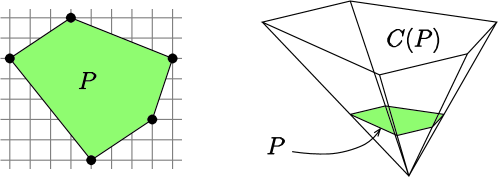
Figure 1: Toric diagram $P$ and the cone $C(P)$

A toric diagram $P\subset\mathbb{R}^{3}$ is a two dimensional convex integral polygon embedded into height one; the coordinates of each vertex is of the form $(*,*,1)\in\mathbb{Z}^{3}$ (Figure 1). Let ${\mathcal{T}}$ denote the set of toric diagrams. For an $n$-gon $P\in{\mathcal{T}}$, denote its vertices by $\bm{v}_{1},\bm{v}_{2},\dots,\bm{v}_{n}$ in counter-clockwise order, so that

$$\left\langle\bm{v}_{i},\bm{v}_{j},\bm{v}_{k}\right\rangle>0,\qquad(1\leq i<j<k\leq n).$$

Here and throughout this paper, $\left\langle\bm{u},\bm{v},\bm{w}\right\rangle$ denotes the determinant of the $3\times 3$ matrix whose columns are $\bm{u},\bm{v},\bm{w}\in{\mathbb{R}}^{3}$. We adopt the convention that the indices are defined modulo $n$, $\bm{v}_{i}=\bm{v}_{i+n}$; thus $\left\langle\bm{v}_{i-1},\bm{v}_{i},\bm{v}_{i+1}\right\rangle>0$ for all $i$. The cone $C(P)$ over the base $P$ defined by

$$C(P):={\mathbb{R}}_{\geq 0}\bm{v}_{1}+\dots+{\mathbb{R}}_{\geq 0}\bm{v}_{n}.$$

will be important for the relation with volume minimization (see Section 9).

With each toric diagram $P\in{\mathcal{T}}$ there is associated a quiver gauge theory. A quiver is a directed graph encoding a gauge theory which gives rise to a SCFT. For our purpose, however, a specific form of the quiver is not needed. Let $N_{\mathrm{gauge}}$ and $N_{\mathrm{matter}}$ denote the number of the vertices and the edges of the quiver, respectively. Each vertex is in one-to-one correspondence with a $U(N)$ factor of the total gauge group $U(N)^{N_{\mathrm{gauge}}}$; each edge represents a chiral bi-fundamental field. The numbers $N_{\mathrm{gauge}}$ and $N_{\mathrm{matter}}$ can be extracted directly from the toric diagram $P$:

$$N_{\mathrm{gauge}} = \sum_{1\leq i\leq n}\left\langle\bm{v}_{i},\bm{v}_{i+1},\bm{e}_{3}\right\rangle=2\mathrm{Area}(P),$$

$$N_{\mathrm{matter}} = \sum_{1\leq i<j\leq n}|\left\langle\bm{v}_{i}-\bm{v}_{i-1},\bm{v}_{j}-\bm{v}_{j-1},\bm{e}_{3}\right\rangle|.$$ (2)

Here $|~{}~{}|$ denotes the usual absolute value and $\bm{e}_{3}$ is the unit vector $(0,0,1)\in{\mathbb{Z}}^{3}$.

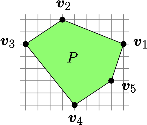
$$\begin{array}[]{|c|c|c|}\hline\cr(i,j)&\mbox{multiplicity}&\mbox{R-charge}\\ \hline\cr(1,2)&17&\phi^{1}\\ \hline\cr(1,3)&\phantom{0}7&\phi^{1}+\phi^{2}\\ \hline\cr(2,3)&16&\phi^{2}\\ \hline\cr(2,4)&17&\phi^{2}+\phi^{3}\\ \hline\cr(3,4)&23&\phi^{3}\\ \hline\cr(4,1)&17&\phi^{4}+\phi^{5}\\ \hline\cr(4,5)&23&\phi^{4}\\ \hline\cr(5,1)&\phantom{0}7&\phi^{5}\\ \hline\cr(5,2)&16&\phi^{5}+\phi^{1}\\ \hline\cr\end{array}$$

Figure 2: An example of toric diagram and the chiral fields of the associated quiver gauge theory

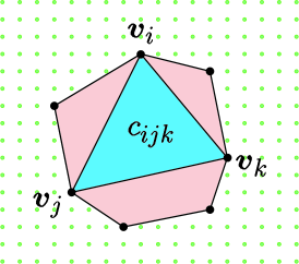
Figure 3: The coefficient $c_{ijk}$.

The $R$-charges of chiral bi-fundamental fields are given as follows. Let $\mathcal{B}$ be the set of all the unordered pairs of edges of $P$. An element $\{\{\bm{v}_{i-1},\bm{v}_{i}\},\{\bm{v}_{j-1},\bm{v}_{j}\}\}$ of $\mathcal{B}$ will be simply denoted by $(i,j)$, with the convention that the oriented edge $(\bm{v}_{i-1},\bm{v}_{i})$ can be rotated to $(\bm{v}_{j-1},\bm{v}_{j})$ in the counter-clockwise direction with an angle $\leq 180^{\circ}$. For each $(i,j)\in\mathcal{B}$, we introduce a chiral field $\Phi_{(i,j)}$ of $R$-charge

$$R(\Phi_{(i,j)}):=\phi^{i}+\phi^{i+1}+\dots+\phi^{j-1}$$

with the multiplicity

$$\mu_{(i,j)}:=\left\langle\bm{v}_{i}-\bm{v}_{i-1},\bm{v}_{j}-\bm{v}_{j-1},\bm{e}_{3}\right\rangle.$$

By our orientation convention, $\mu_{(i,j)}$ are non-negative. The $R$-charges $\phi^{i}$ are constrained as

$$\phi^{1}+\phi^{2}+\dots+\phi^{n}=2.$$ (3)

The $a$-function of the quiver gauge theory is then given by

$$a(\phi)=\frac{9N^{2}}{32}\biggl{[}N_{\mathrm{gauge}}+\sum_{(i,j)\in\mathcal{B}}\mu_{(i,j)}\bigl{(}R(\Phi_{(i,j)})-1\bigr{)}^{3}\biggr{]}.$$ (4)

Figure 2 is an example of a toric diagram and the chiral field content of the corresponding quiver gauge theory.

Benvenuti, Zayas, Tachikawa [17] and Lee, Rey [18] have shown that under the constraint (3), the $a$-function (4) can be neatly rewritten as

$$a(\phi)=\frac{9}{32}\frac{N^{2}}{2}\sum_{i,j,k=1}^{n}c_{ijk}\,\phi^{i}\phi^{j}\phi^{k}$$ (5)

where

$$c_{ijk}=|\det(\bm{v}_{i},\bm{v}_{j},\bm{v}_{k})|$$ (6)

is proportional to the area of the triangle with vertices $\bm{v}_{i},\bm{v}_{j},\bm{v}_{k}$ sitting inside $P$ (see Figure 3). The formulas (5) and (6) make the starting point our investigation.

3 Mathematical setup and main results

In this section, we discuss the mathematical formulation of $a$-maximization and state our main theorems.

Let $P\in{\mathcal{T}}$ be a toric diagram and $\bm{v}_{1},\bm{v}_{2},\dots,\bm{v}_{n}$ the vertices of $P$ in counter-clockwise order, as described in Section 2. Define a homogeneous cubic polynomial $\hat{F}_{P}$ in $\phi=(\phi^{1},\phi^{2},\dots,\phi^{n})$ by

$$\hat{F}_{P}(\phi)=\sum_{1\leq i<j<k\leq n}|\det(\bm{v}_{i},\bm{v}_{j},\bm{v}_{k})|\,\phi^{i}\phi^{j}\phi^{k}.$$ (7)

Choose a real constant $r>0$ and fix it. Let $\rho:{\mathbb{R}}_{\geq 0}^{n}\to{\mathbb{R}}$ denote the linear function

$$\rho(\phi):=\phi^{1}+\dots+\phi^{n}$$

and set

$$\Gamma_{n}:=\rho^{-1}(r)=\biggl{\{}\phi=(\phi^{1},\dots,\phi^{n})\in{\mathbb{R}}_{\geq 0}^{n}~{}:\;\sum_{i=1}^{n}\phi^{i}=r\biggr{\}},$$

which is an $n{-}1$ dimensional simplex. Its relative interior i.e. the interior as a topological subspace of its affine hull will be denoted by

$$\mathop{\rm relint}(\Gamma_{n})=\{\phi=(\phi^{1},\dots,\phi^{n})\in{\mathbb{R}}^{n}\,:\,\sum_{i=1}^{n}\phi^{i}=r,\;\phi^{i}>0\}.$$

The function $F_{P}$ is defined to be the restriction of $\hat{F}_{P}$ to $\Gamma_{n}$. Obviously, $F_{P}$ is a model for $a$-function (5), and $\Gamma_{n}$ (or $\mathop{\rm relint}(\Gamma_{n})$) represents a physically allowed region of $R$-charges. The choice of $r$ is not important for $a$-maximization; the homogeneity $\hat{F}_{P}(\lambda\phi)=\lambda^{3}\hat{F}_{P}(\phi)$ allows us to choose $r$ any positive real number. Usually we set $r=2$ to match the convention (3).

For each toric diagram $P\in{\mathcal{T}}$, define its modulus by

$$\mathfrak{M}(P):=\biggl{(}\frac{3}{r}\biggr{)}^{3}\max_{\phi\in\rho^{-1}(r)}\hat{F}_{P}(\phi).$$

The modulus $\mathfrak{M}(P)$ is independent of $r$ and is normalized so that the smallest toric diagram $P=\{\bm{v}_{1}=(0,0,1),\bm{v}_{2}=(1,0,1),\bm{v}_{3}=(0,1,1)\}$ has unit modulus. This $\mathfrak{M}$ is the quantity of our primary interest.

Let $G$ be the subgroup of $GL(3,{\mathbb{Z}})$ which leave invariant the set of lattice points on hyperplane $(*,*,1)$. $G$ induces integral affine transformations on this hyperplane: $G\simeq GL(2,{\mathbb{Z}})\ltimes{\mathbb{Z}}^{2}$. $G$ acts naturally on the set of toric diagrams ${\mathcal{T}}$: for $g\in G$ and a polygon $P$ with vertices $\bm{v}_{1},\cdots,\bm{v}_{n}$, $g(P)$ is the polygon with vertices $g(\bm{v}_{1}),\cdots,g(\bm{v}_{n})$. The $G$-action defines an equivalence relation $\simeq$ on ${\mathcal{T}}$:

$$P\simeq Q\quad\stackrel{{\scriptstyle\mathrm{def}}}{{\Longleftrightarrow}}\quad\exists\,g\in G\mbox{~{}such that~{}}g(P)=Q.$$

We denote by $[P]$ the equivalence class of $P$. The functions $\hat{F}_{P}$ are $G$-invariant, $F_{P}(\phi)$ $=F_{g(P)}(\phi)$, because $\hat{F}_{P}$ depends on $P$ only through the areas of triangles inscribed in $P$. The modulus $\mathfrak{M}$ is thus well-defined on ${\mathcal{T}}/\simeq$. In the physical context, two $G$-equivalent toric diagrams $P$ and $Q$ are associated with the identical quiver gauge theory and the same dual Sasaki-Einstein geometry, so there is no reason to distinguish the two.

In connection with RG flow, it is interesting to compare $\mathfrak{M}(P)$ and $\mathfrak{M}(P^{\prime})$ for toric diagrams $P$ and $P^{\prime}$ which are not necessarily $G$-equivalent. The inclusion relation $\subset$ on ${\mathcal{T}}$ naturally induces a partial order $\preceq$ on ${\mathcal{T}}/\simeq$, namely,

$$[P]\preceq[P^{\prime}]\;\stackrel{{\scriptstyle\mathrm{def}}}{{\Longleftrightarrow}}\;\exists\,Q,Q^{\prime}\in{\mathcal{T}}\mbox{~{}such that~{}}P\simeq Q,\;P^{\prime}\simeq Q^{\prime},\;Q\subset Q^{\prime}.$$ (8)

The basic question we shall be concerned with is the existence and uniqueness of the critical point of $F_{P}$; we want to establish this as a mathematical fact independent of duality conjectures. This problem is not so simple as it may appear at a first glance. For example, consider the function

$$\hat{F}_{P}(\phi)=2\phi^{1}\phi^{2}\phi^{3}+4\phi^{1}\phi^{2}\phi^{4}+3\phi^{1}\phi^{3}\phi^{4}+\phi^{2}\phi^{3}\phi^{4}$$

which corresponds to the toric diagram $P=\{(2,3,1),(0,1,1),(0,0,1),(1,0,1)\}$. This $\hat{F}_{P}$ has a unique critical point in $\mathop{\rm relint}(\Gamma_{4})$. However,

$$\hat{F}(\phi)=2\phi^{1}\phi^{2}\phi^{3}+8\phi^{1}\phi^{2}\phi^{4}+3\phi^{1}\phi^{3}\phi^{4}+\phi^{2}\phi^{3}\phi^{4}\qquad\qquad\quad~{}$$

has no critical points in $\mathop{\rm relint}(\Gamma_{4})$; it is maximized at $\phi=(\frac{r}{3},\frac{r}{3},0,\frac{r}{3})\in\partial\Gamma_{4}$ but this is not a critical point. On the other hand,

$$\hat{F}(\phi) = \,4\phi^{1}\phi^{2}\phi^{3}+2\phi^{1}\phi^{2}\phi^{4}+9\phi^{1}\phi^{3}\phi^{4}+7\phi^{2}\phi^{3}\phi^{4}$$

$$+4\phi^{1}\phi^{3}\phi^{5}+\phi^{2}\phi^{3}\phi^{5}+\phi^{1}\phi^{4}\phi^{5}+10\phi^{2}\phi^{4}\phi^{5}+4\phi^{3}\phi^{4}\phi^{5}$$

has two critical points in $\mathop{\rm relint}(\Gamma_{5})$; one is a local maximum and the other is a saddle point. Consequently the conditions such as

• $c_{ijk}$ are non-negative integers,

• $c_{ijk}$ is invariant under any permutation of indices $i,j,k$, and

• $c_{ijk}=0$ unless $i,j,k$ are distinct,

are not enough to guarantee the existence and uniqueness of the critical point in $\mathop{\rm relint}(\Gamma_{n})$. The fact that the coefficients $c_{ijk}$ are given by the areas of triangles will be heavily used in this paper.

Our main results are as follows:

Theorem 3.1 (Theorem 6.4)

The function $F_{P}:\Gamma_{n}\to{\mathbb{R}}$ has a unique critical point $\phi_{*}$ in $\mathop{\rm relint}(\Gamma_{n})$ and $\phi_{*}$ is also the unique global maximum of $F_{P}$.

Theorem 3.2 (Theorem 7.1)

The critical point $\phi_{*}$ satisfies the universal bound

$$0<\phi_{*}^{i}\leq\frac{r}{3}\qquad(i=1,\dots,n).$$

Here, the equality $\phi_{*}^{i}=\frac{r}{3}$ holds for some $i$ if and only if $n=3$.

Theorem 3.3 (Theorem 8.5)

The maximum value of $F_{P}$ is monotone in the following sense: Suppose $P$ and $P^{\prime}$ are toric diagrams satisfying $[P]\preceq[P^{\prime}]$. Then $\mathfrak{M}(P)\leq\mathfrak{M}(P^{\prime})$. The equality holds if and only if $P\simeq P^{\prime}$.

Some comments are in order here. The unitarity of the representation of superconformal algebra $SU(2,2|1)$ requires that all gauge invariant chiral operators must have $U(1)_{R}$ charge $R\geq\frac{2}{3}$ [4, 5]. Theorem 3.2, however, yields opposite inequalities $\phi^{i}_{*}\leq\frac{2}{3}$ in the conventional normalization $r=2$ (see (3)). This is not a contradiction because $\phi_{*}^{i}$ are $R$ charges of gauge non-invariant bi-fundamental fields.

Theorem 3.3 can be regarded as a combinatorial analogue of “$a$-theorem”: the $a$-function always decreases whenever the toric diagram shrinks.

There are two key ingredients in the proof of the main results. First, $a$-function is identified with the volume of a three dimensional polytope called “zonotope” (Proposition 4.2); Brunn-Minkowski inequality asserts that (cubic root of) volume function is a concave function on the space of polytopes. This concavity guarantees the uniqueness of the critical point (Proposition 5.5). Second key point is to show the monotonicity of modulus $\mathfrak{M}$ under simple change of the toric diagrams, e.g. deleting a vertex. This property is also used to prove the existence of the critical point.

Here is an application of our results. The uniqueness of the maximizer implies that there is no spontaneous symmetry break down in $a$-maximization:

Corollary 3.4

If a nontrivial element $g$ of $G$ fixes a toric diagram $P$, then the critical point $\phi_{*}$ of $F_{P}$ is also fixed by $g$.

4 Polytopes and Zonotopes

Let ${\mathbb{R}}^{d}$ denote a $d$-dimensional real vector space. A subset $C\subset{\mathbb{R}}^{d}$ is called convex if $(1-\lambda)\bm{x}+\lambda\bm{y}\in C$ whenever $\bm{x},\bm{y}\in C$ and $0\leq\lambda\leq 1$. For any set $S\subset{\mathbb{R}}^{d}$, its convex hull $\mathop{\rm conv}(S)$ is, by definition, the smallest convex set containing $S$:

$$\mathop{\rm conv}(S):=\{\lambda\bm{x}+(1-\lambda)\bm{y}\in{\mathbb{R}}^{d}~{}:~{}\bm{x},\bm{y}\in S,\;0\leq\lambda\leq 1\}.$$

A polytope is the convex hull $\mathop{\rm conv}(S)$ of a finite set $S$ in ${\mathbb{R}}^{d}$.

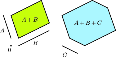
Figure 4: Minkowski sums

The Minkowski sum, or vector sum, of two subsets $A$ and $B$ in ${\mathbb{R}}^{d}$ is (see Figure 4)

$$A+B:=\{\bm{x}+\bm{y}~{}:~{}\bm{x}\in A,~{}\bm{y}\in B\},$$

whereas the dilatation by the factor $r\geq 0$ is

$$rA=\{r\bm{x}~{}:~{}\bm{x}\in A\}.$$

If $A$ and $B$ are polytopes, then $A+B$, $rA$ are also polytopes. Let $\mathcal{P}^{d}$ denote the family of all convex polytopes in ${\mathbb{R}}^{d}$. Two basic operations, Minkowski sum and dilatation, make the family $\mathcal{P}^{d}$ a convex set: for any $A,B\in\mathcal{P}^{d}$ and non-negative numbers $\alpha,\beta$ such that $\alpha+\beta=1$ one has $\alpha A+\beta B\in\mathcal{P}^{d}$.

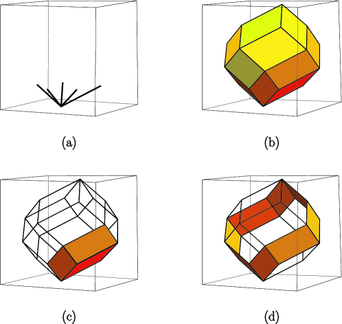
Figure 5: A zonotope ($d=3$, $n=5$) : generators (a), zonotope (b), cube (c) and zone (d).

Let $S_{1},\dots,S_{n}$ be $n$ line segments, each of non-zero length, in ${\mathbb{R}}^{d}$. The polytope ${\mathcal{Z}}$ defined as the Minkowski sum

$${\mathcal{Z}}=S_{1}+\dots+S_{n}$$

is called a zonotope and $S_{1},\dots,S_{n}$ are called its generators (Figure 5). For a finite collection of vectors $X=\{\bm{x}_{1},\dots,\bm{x}_{n}\}\subset{\mathbb{R}}^{d}$, we put $S_{i}=\mathop{\rm conv}(\bm{0},\bm{x}_{i})\;(i=1,\dots,n)$, and write ${\mathcal{Z}}[X]$ the corresponding zonotope. Equivalently,

$${\mathcal{Z}}[X]=\{\bm{x}\in{\mathbb{R}}^{d}~{}:~{}\bm{x}=\lambda_{1}\bm{x}_{1}+\dots+\lambda_{n}\bm{x}_{n},~{}0\leq\lambda_{i}\leq 1,~{}i=1,\dots,n\}.$$

The zonotope ${\mathcal{Z}}[X]$ is the image of an $n$-dimensional cube $[0,1]^{n}$ under a linear projection $\pi:{\mathbb{R}}^{n}\to{\mathbb{R}}^{d}$ defined by the $d\times n$ matrix $X$. ${\mathcal{Z}}[X]$ may also be defined as the convex hull of $2^{n}$ points

$$\{\bm{x}_{i_{1}}+\bm{x}_{i_{2}}+\dots+\bm{x}_{i_{k}}\in{\mathbb{R}}^{d}~{}:~{}1\leq i_{1}<i_{2}<\dots<i_{k}\leq n,~{}k=0,1,\dots,n\}.$$

${\mathcal{Z}}[X]$ is centrally symmetric, and its center is located at $\frac{1}{2}(\bm{x}_{1}+\dots+\bm{x}_{n})$.

The zonotope ${\mathcal{Z}}[X]$ can be decomposed into $\pmatrix{n\cr d}$ $d$-dimensional parallelepipeds called cubes, each of which is a translation of

$$Q_{i_{1},\dots,i_{d}}:=\mathop{\rm conv}(\bm{0},\bm{x}_{i_{1}})+\mathop{\rm conv}(\bm{0},\bm{x}_{i_{2}})+\dots+\mathop{\rm conv}(\bm{0},\bm{x}_{i_{d}}).$$

The crucial fact is that, although such decomposition is not unique, all $d$-tuples $\{\bm{x}_{i_{1}},$ $\dots,$ $\bm{x}_{i_{d}}\}$ $\subset X$ appear exactly once in any decomposition. Since the volume of each cube $Q_{i_{1},\dots,i_{d}}$ is simply given by $\mathop{\rm vol}(Q_{i_{1},\dots,i_{d}})=|\det(\bm{x}_{i_{1}},\dots,\bm{x}_{i_{d}})|$, this leads to the following volume formula for zonotopes, which will play a crucial role in this paper.

Theorem 4.1 (Shephard [19], attributed to McMullen)

$$\mathop{\rm vol}({\mathcal{Z}}[X])=\sum_{1\leq i_{1}<\dots<i_{d}\leq n}|\det(\bm{x}_{i_{1}},\dots,\bm{x}_{i_{d}})|.$$ (9)

In the rest of this paper, we will specialize to $d{=}3$ case, i.e. three dimensional zonotopes. If no three of the $n$ vectors $\bm{x}_{1},\dots,\bm{x}_{n}$ are coplanar, all the facets (i.e. two dimensional faces) of ${\mathcal{Z}}[X]$ are parallelograms. For a given generator $\bm{x}_{s}$, the faces which has a edge parallel to $\bm{x}_{s}$ form a zone going around a zonotope. Each zone consists of $n{-}1$ pairs of opposite faces, there are altogether $n(n{-}1)/2$ pairs of opposite faces, $n(n{-}1)$ pairs of opposite edges, and therefore $n(n{-}1)/2+1$ pairs of opposite vertices.

The next Proposition is our key observation, which immediately follows by comparing (7) and (9).

Proposition 4.2

Let $P\in{\mathcal{T}}$ be a toric diagram with vertices $\bm{v}_{1},\dots,\bm{v}_{n}$. The function $\hat{F}_{P}(\phi)$ defined in (7) is equal to the volume of the zonotope

$${\mathcal{Z}}_{P}(\phi):=\phi^{1}\mathop{\rm conv}(\bm{0},\bm{v}_{1})+\phi^{2}\mathop{\rm conv}(\bm{0},\bm{v}_{2})+\dots+\phi^{n}\mathop{\rm conv}(\bm{0},\bm{v}_{n}).$$ (10)

The trial $a$-function (5) is therefore given by

$$a(\phi)=\frac{27}{32}N^{2}\hat{F}_{P}(\phi)=\frac{27}{32}N^{2}\mathop{\rm vol}({\mathcal{Z}}_{P}(\phi)).$$

5 Uniqueness of the critical point

In this section, the uniqueness of the critical point of $\hat{F}_{P}$ is proved; the existence is shown in the next section.

A real-valued function $f$ on a convex set $C$ is concave if

$$f((1-\lambda)x+\lambda y)\geq(1-\lambda)f(x)+\lambda f(y)$$

for all $x,y\in C$ and $0<\lambda<1$. If the above inequality can be replaced by

$$f((1-\lambda)x+\lambda y)>(1-\lambda)f(x)+\lambda f(y),$$

then $f$ is strictly concave. We will use the following well known properties of concave functions:

Theorem 5.1

Any local maximizer of a concave function $f$ defined on a convex set $C$ of ${\mathbb{R}}^{n}$ is also a global maximizer of $f$. If in addition $f$ is differentiable, then any stationary point is a global maximizer of $f$. Any local maximizer of a strictly concave function $f$ defined on a convex set $C$ of ${\mathbb{R}}^{n}$ is the unique strict global maximizer of $f$ on $C$.

Recall that the family $\mathcal{P}^{d}$ of polytopes in ${\mathbb{R}}^{d}$ is a convex set under the operations Minkowski sum and dilatation. Thus it makes sense to talk about the concavity of a function defined on $\mathcal{P}^{d}$, such as volume function. The following is a fundamental result in the theory of convex bodies (for extensive survey, see [20, 21]).

Theorem 5.2 (Brunn-Minkowski inequality)

The $d$-th root of volume is a concave function on the family of convex bodies in ${\mathbb{R}}^{d}$. More precisely, for convex bodies $A,B\subset{\mathbb{R}}^{d}$ and for $0\leq\lambda\leq 1$,

$$\left(\mathop{\rm vol}((1-\lambda)A+\lambda B)\right)^{1/d}\geq(1-\lambda)\left(\mathop{\rm vol}(A)\right)^{1/d}+\lambda\left(\mathop{\rm vol}(B)\right)^{1/d}.$$

Equality for some $0<\lambda<1$ holds if and only if $A$ and $B$ either lie in parallel hyperplanes or are homothetic.

In Proposition 4.2, $F_{P}(\phi)$ is identified with the volume of a three dimensional zonotope. Actually, we are interested in the “family” of zonotopes ${\mathcal{Z}}_{P}(\phi)$ parametrized by $\phi=(\phi^{1},\dots,\phi^{n})\in\Gamma_{n}$. In order to apply Brunn-Minkowski inequality to this family, let us investigate under what conditions two zonotopes are homothetic to each other.

Lemma 5.3

For $\phi,\phi^{\prime}\in{\mathbb{R}}_{\geq 0}^{n}$, two zonotopes ${\mathcal{Z}}_{P}(\phi)$, ${\mathcal{Z}}_{P}(\phi^{\prime})$ of nonzero volume are homothetic if and only if $\phi=\kappa\phi^{\prime}$ for some $\kappa>0$. In particular, two zonotopes ${\mathcal{Z}}_{P}(\phi)$, ${\mathcal{Z}}_{P}(\phi^{\prime})$ with $\phi,\phi^{\prime}\in\Gamma_{n}$ are homothetic if and only if $\phi=\phi^{\prime}$.

Proof. Suppose ${\mathcal{Z}}_{P}(\phi)$ and ${\mathcal{Z}}_{P}(\phi^{\prime})$ are homothetic. By assumption, they have nonzero volume and cannot be in a hyperplane. Thus there exists $\kappa>0$ and $t\in{\mathbb{R}}^{3}$ such that ${\mathcal{Z}}_{P}(a)=\kappa{\mathcal{Z}}_{P}(b)+t$. In fact $t=0$ because both zonotopes have $O=(0,0,0)$ as the bottom vertex. Each of them have a unique edge starting from $O$ and parallel to $\bm{v}_{i}$ for all $i$. Homothethy implies $\phi^{i}\mathop{\rm conv}(\bm{0},\bm{v}_{i})=\kappa\phi^{\prime i}\mathop{\rm conv}(\bm{0},\bm{v}_{i})$, so $\phi^{i}=\kappa\phi^{\prime i}$ holds for all $i$. In particular, if $\phi,\phi^{\prime}\in\Gamma_{n}$, then $r=\rho(\phi)=\rho(\kappa\phi^{\prime})=\kappa\rho(\phi^{\prime})=\kappa r$, so $\kappa=1$. $\Box$

Here we come to the key point of our analysis.

Proposition 5.4

The function

$$\bigl{(}\hat{F}_{P}(\phi)\bigr{)}^{1/3}=\left(\mathop{\rm vol}{\mathcal{Z}}_{P}(\phi)\right)^{1/3}~{}:~{}{\mathbb{R}}_{\geq 0}^{n}\to{\mathbb{R}}$$ (11)

is concave. Moreover, its restriction, $(F_{P})^{1/3}:\Gamma_{n}\to{\mathbb{R}}$ is strictly concave.

Proof. Let us denote the function (11) by $f_{P}$. It suffices to show that for any $a=(a^{1},\dots,a^{n})$, $b=(b^{1},\dots,b^{n})$ $\in{\mathbb{R}}_{\geq 0}^{n}$,

$$f_{P}((1-\lambda)a+\lambda b)\geq(1-\lambda)f_{P}(a)+\lambda f_{P}(b)\qquad(0\leq\lambda\leq 1)$$

and the equality holds if and only if $a=\kappa\,b$ for some $\kappa>0$. One can easily check that

$$\sum_{i=1}^{n}((1-\lambda)a^{i}+\lambda b^{i})\mathop{\rm conv}(\bm{0},\bm{v}_{i})=(1-\lambda)\sum_{i=1}^{n}a^{i}\mathop{\rm conv}(\bm{0},\bm{v}_{i})+\lambda\sum_{i=1}^{n}b^{i}\mathop{\rm conv}(\bm{0},\bm{v}_{i})$$

holds as an equality in $\mathcal{P}^{d}$. Using the notation (10), this is written as

$${\mathcal{Z}}_{P}((1-\lambda)a+\lambda b)=(1-\lambda){\mathcal{Z}}_{P}(a)+\lambda{\mathcal{Z}}_{P}(b)$$

Then the claim immediately follows from Theorem 5.2 and Lemma 5.3. $\Box$

Since the function $x\mapsto x^{1/3}:{\mathbb{R}}_{\geq 0}\to{\mathbb{R}}_{\geq 0}$ is a strictly increasing function, $\hat{F}_{P}$ is maximal (resp. critical) at $\phi$ if and only if $(\hat{F}_{P})^{1/3}$ is maximal (resp. critical) at $\phi$. Combining Theorem 5.1 and Proposition 5.4, we have established the uniqueness of the solution to $a$-maximization:

Proposition 5.5

Suppose $\phi_{*}$ is a critical point or a local maximum of $F_{P}:\Gamma_{n}\to{\mathbb{R}}$. Then $\phi_{*}$ is the unique critical point and is also the global maximum over $\Gamma_{n}$.

A remark is in order here: $F_{P}$ is not necessarily concave although the cubic root $(F_{P})^{1/3}$ is. The conifold $\bm{v}_{1}=(1,1,1),\bm{v}_{2}=(1,0,1),\bm{v}_{3}=(1,0,0),\bm{v}_{4}=(1,1,0)$,

$$F_{P}(\phi)=\phi^{2}\phi^{3}\phi^{4}+\phi^{1}\phi^{3}\phi^{4}+\phi^{1}\phi^{2}\phi^{4}+\phi^{1}\phi^{2}\phi^{3},\qquad(\phi^{1}+\phi^{2}+\phi^{3}+\phi^{4}=2)$$

is already a counterexample; the Hessian of $F_{P}$ at $\phi=(\frac{1}{7},\frac{1}{7},\frac{3}{7},\frac{9}{7})$ is not negative definite.

6 Existence of the critical point

This section is devoted to the proof of Theorem 3.1 (Theorem 6.4). The key idea is as follows. The continuous function $F_{P}$ always has a global maximum on the closed set $\Gamma_{n}$. If the maximum point is in $\mathop{\rm relint}(\Gamma_{n})$, then from Proposition 5.5 it is also a critical point and there is no other local maxima. But if the maximum point is on the boundary $\partial\Gamma_{n}$, it is not necessarily a critical point — physical SCFT. Therefore to establish Theorem 3.1, it suffices to show that a point on the boundary $\partial\Gamma_{n}$ can never be a local maximum of $F_{P}$.

For this purpose, we investigate the behavior of the maximum values under the change of toric diagrams. More precisely we will prove the following

Proposition 6.1

Let $P$ be a toric diagram with vertices $\bm{v}_{1},\dots,\bm{v}_{n}$ in counterclockwise order. Let $Q$ be a toric diagram obtained by deleting $\bm{v}_{n}$ from $P$, i.e. the convex hull of $n{-}1$ vertices $\bm{v}_{1},\dots,\bm{v}_{n-1}$ as in Figure 6. Then, for any $\phi\in\mathop{\rm relint}(\Gamma_{n-1})$, there exits $\psi\in\mathop{\rm relint}(\Gamma_{n})$ such that $F_{Q}(\phi)<F_{P}(\psi)$.

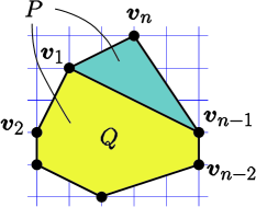
Figure 6: Deleting a vertex

Note that under the natural inclusion

$$\Gamma_{n-1}\subset\Gamma_{n},\qquad\phi=(\phi^{1},\dots,\phi^{n-1})\mapsto(\phi^{1},\dots,\phi^{n-1},0),$$

the point $\phi\in\mathop{\rm relint}(\Gamma_{n-1})$ corresponds to a point on the boundary facet $\{\phi^{n}=0\}$ of $\Gamma_{n}$, and $F_{Q}$ is none other than the restriction of $F_{P}$ to this facet. Clearly, any boundary point of $\Gamma_{n}$ is obtained in this manner. Thus Proposition 6.1 immediately implies

Corollary 6.2

No boundary point of $\Gamma_{n}$ can be a local maximum of $F_{P}:\Gamma_{n}\to{\mathbb{R}}$.

Corollary 6.3

Suppose a toric diagram $Q$ is obtained from another toric diagram $P$ by removing one vertex, then $\mathfrak{M}(Q)<\mathfrak{M}(P)$.

By the argument given in the first paragraph of this section, we deduce from Corollary 6.2 the following

Theorem 6.4

Suppose $P$ is a toric diagram with vertices $\bm{v}_{1},\dots,\bm{v}_{n}$. Then $F_{P}:\Gamma_{n}\to{\mathbb{R}}$ has a unique critical point $\phi_{*}$ in $\mathop{\rm relint}(\Gamma_{n})$ and $\phi_{*}$ is also the unique global maximum of $F_{P}$.

Let us turn to the proof of Proposition 6.1. Our strategy is to show that for any $\phi\in\mathop{\rm relint}(\Gamma_{n-1})\subset\partial\Gamma_{n}$ there is at least one “inward” direction in which $F_{P}$ is strictly increasing. Consider two straight paths $\psi_{I}(t),\psi_{II}(t)$ in $\Gamma_{n}$ emanating from the boundary point $\phi$, defined by

$$\psi_{I}^{i}(t)=\left\{\begin{array}[]{ll}\phi^{1}-t&\mbox{if $i=1$},\\ t&\mbox{if $i=n$},\\ \phi^{i}&\mbox{otherwise},\\ \end{array}\right.\qquad\mbox{and}\qquad\psi_{II}^{i}(t)=\left\{\begin{array}[]{ll}\phi^{n-1}-t&\mbox{if $i=n-1$},\\ t&\mbox{if $i=n$},\\ \phi^{i}&\mbox{otherwise},\end{array}\right.$$

for $0\leq t\leq\min(\phi^{1},\phi^{n-1})$. If either $\frac{d}{dt}\big{|}_{t=0}F_{P}(\psi_{I}(t))>0$ or $\frac{d}{dt}\big{|}_{t=0}F_{P}(\psi_{II}(t))>0$ is proved, then we are done.

Note that for three vectors $\bm{a},\bm{b},\bm{c}\in{\mathbb{R}}^{3}$, the relation $\left\langle\bm{a},\bm{b},\bm{c}\right\rangle=(\bm{a}\times\bm{b})\cdot\bm{c}$ holds, where $\bm{a}\times\bm{b}$ denotes the cross product and $\cdot$ is the standard inner product. Let $\bm{\xi}\in{\mathbb{R}}^{3}$ be a vector defined by

$$\bm{\xi}=\sum_{1\leq i<j\leq n-1}\phi^{i}\phi^{j}\bm{v}_{i}\times\bm{v}_{j}.$$

It is easy to see

$$\frac{d}{dt}\Big{|}_{t=0}F_{P}(\psi_{I}(t)) = \sum_{1\leq i<j\leq n-1}(c_{ij\,n}-c_{ij\,1})\phi^{i}\phi^{j}=\bm{\xi}\cdot(\bm{v}_{n}-\bm{v}_{1}),$$

$$\frac{d}{dt}\Big{|}_{t=0}F_{P}(\psi_{II}(t)) = \sum_{1\leq i<j\leq n-1}(c_{ij\,n}-c_{ij\,n{-}1})\phi^{i}\phi^{j}=\bm{\xi}\cdot(\bm{v}_{n}-\bm{v}_{n-1}).$$

Thus it suffices to show either $\bm{\xi}\cdot(\bm{v}_{n}-\bm{v}_{1})>0$ or $\bm{\xi}\cdot(\bm{v}_{n}-\bm{v}_{n-1})>0$ holds.

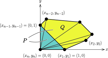
Figure 7: $(x,y)$-coordinates.

Let us choose three vectors $\bm{v}_{1},\bm{v}_{n-1},\bm{v}_{n}$ as a basis of ${\mathbb{R}}^{3}$ and express other $\bm{v}_{i}$’s as

$$\bm{v}_{i}=x_{i}\bm{v}_{1}+y_{i}\bm{v}_{n-1}+(1-x_{i}-y_{i})\bm{v}_{n}.$$

In the affine coordinates $(x_{i},y_{i})$, the toric diagram $P$ and $Q$ looks like polygons sitting in the first quadrant of ${\mathbb{R}}^{2}$, as depicted in Figure 7. Note that $x_{i}y_{j}>x_{j}y_{i}$ for all $1\leq i<j\leq n-1$.

A straightforward calculation shows

$$\bm{\xi}\cdot(\bm{v}_{n}-\bm{v}_{1}) = \det(\bm{v}_{1},\bm{v}_{n-1},\bm{v}_{n})\sum_{1\leq i<j\leq n-1}\phi^{i}\phi^{j}(y_{j}-y_{i}),$$

$$\bm{\xi}\cdot(\bm{v}_{n}-\bm{v}_{n-1}) = \det(\bm{v}_{1},\bm{v}_{n-1},\bm{v}_{n})\sum_{1\leq i<j\leq n-1}\phi^{i}\phi^{j}(x_{i}-x_{j}).$$

Since $\det(\bm{v}_{1},\bm{v}_{n-1},\bm{v}_{n})>0$, the claim follows from the next lemma.

Lemma 6.5

Let $\phi^{1},\phi^{2},\dots,\phi^{n-1}$ be positive numbers and

$$(x_{1},y_{1}),\;(x_{2},y_{2}),\;\dots\;,(x_{n-2},y_{n-2}),\;(x_{n-1},y_{n-1})$$

be $n-1$ points in ${\mathbb{R}}_{\geq 0}^{2}$ satisfying

$$x_{i}y_{j}-x_{j}y_{i}>0\qquad(1\leq i<j\leq n-1).$$ (12)

Then, at least one of the following inequalities holds:

$$\sum_{1\leq i<j\leq n-1}\phi^{i}\phi^{j}(x_{i}-x_{j})>0,\qquad\mbox{or}\quad\sum_{1\leq i<j\leq n-1}\phi^{i}\phi^{j}(y_{j}-y_{i})>0.$$ (13)

Proof. Define $c_{1},c_{2},\dots,c_{n-1}$ by

$$c_{i}=\phi^{i}\biggl{(}\sum_{1\leq j<i}\phi^{j}-\sum_{i<j\leq n-1}\phi^{j}\biggr{)}.$$

Clearly $c_{1}<0$ and $c_{n-1}>0$, and the sequence $\frac{c_{1}}{\phi^{1}},\frac{c_{2}}{\phi^{2}},\dots,\frac{c_{n-1}}{\phi^{n-1}}$ is strictly increasing since $\frac{c_{i+1}}{\phi^{i+1}}-\frac{c_{i}}{\phi^{i}}$ $=\phi^{i}+\phi^{i+1}>0$. Hence there exists $k$ ($2\leq k\leq n-1$) such that $c_{1},c_{2},\dots,c_{k-1}<0$ and $c_{k},c_{k+1},\dots,c_{n-1}\geq 0$. The expressions is (13) can be rewritten as

$$\sum_{1\leq i<j\leq n-1}\phi^{i}\phi^{j}(x_{i}-x_{j}) = -\sum_{i=1}^{n-1}c_{i}x_{i}=\sum_{i=1}^{k-1}|c_{i}|x_{i}-\sum_{i=k}^{n-1}|c_{i}|x_{i},$$ (14)

$$\sum_{1\leq i<j\leq n-1}\phi^{i}\phi^{j}(y_{j}-y_{i}) = \sum_{i=1}^{n-1}c_{i}y_{i}=-\sum_{i=1}^{k-1}|c_{i}|y_{i}+\sum_{i=k}^{n-1}|c_{i}|y_{i}.$$ (15)

Suppose that, contrary to our claim, neither of (13) is true. Then (14) and (15) are both non-positive, which means

$$0<\sum_{i=1}^{k-1}|c_{i}|x_{i}\leq\sum_{i=k}^{n-1}|c_{i}|x_{i}\qquad\mbox{and}\qquad 0<\sum_{i=k}^{n-1}|c_{i}|y_{i}\leq\sum_{i=1}^{k-1}|c_{i}|y_{i}.$$ (16)

On the other hand, from (12),

$$\sum_{i=1}^{k-1}|c_{i}|(x_{i}y_{k-1}-x_{k-1}y_{i})\geq 0,\qquad\mbox{and}\qquad\sum_{i=k}^{n-1}|c_{i}|(x_{i}y_{k}-x_{k}y_{i})\leq 0.$$ (17)

It follows from (16) and (17) that

$$\frac{y_{k}}{x_{k}}\leq\frac{\sum_{i=k}^{n-1}|c_{i}|y_{i}}{\sum_{i=k}^{n-1}|c_{i}|x_{i}}\leq\frac{\sum_{i=1}^{k-1}|c_{i}|y_{i}}{\sum_{i=1}^{k-1}|c_{i}|x_{i}}\leq\frac{y_{k-1}}{x_{k-1}},$$

therefore $x_{k-1}y_{k}-x_{k}y_{k-1}\leq 0$. This contradicts (12). $\Box$

7 Bounds on critical points

In this section, we establish Theorem 3.2 (Theorem 7.1). As we will see, an upper bound on the coordinates of the critical point is easily obtained using the interpretation as volumes.

Let $P$ be a toric diagram with vertices $\bm{v}_{1},\dots,\bm{v}_{n}$. As mentioned before, the zonotope ${\mathcal{Z}}_{P}(\phi)$ can be cut into the union of $\pmatrix{n\cr 3}$ cubes and $F_{P}(\phi)=\mathop{\rm vol}({\mathcal{Z}}_{P}(\phi))$ equals the sum of the volumes of all cubes. We arbitrarily fix such a decomposition. For any $s$ ($s=1,\dots,n$), let ${\mathcal{Z}}_{P}^{[s]}(\phi)$ denote the union of those cubes which has at least one face belonging to $s$-th zone. It is obvious that $\mathop{\rm vol}({\mathcal{Z}}_{P}^{[s]}(\phi))\leq\mathop{\rm vol}({\mathcal{Z}}_{P}(\phi))$ for all $s$. The main result of this section is the following

Theorem 7.1

If $\phi_{*}\in\Gamma_{n}=\rho^{-1}(r)$ is the critical point of $F_{P}$, then

$$\phi^{s}_{*}=\frac{r}{3}\cdot\frac{\mathop{\rm vol}({\mathcal{Z}}_{P}^{[s]}(\phi))}{\mathop{\rm vol}({\mathcal{Z}}_{P}(\phi))},\qquad(s=1,\dots,n).$$

In particular, the critical point satisfies the inequalities

$$0<\phi_{*}^{i}\leq\frac{r}{3},\quad(i=1,\dots,n).$$

where the equality $\phi_{*}^{i}=\frac{r}{3}$ holds for some $i$ if and only if $n=3$ i.e. when the toric diagram $P$ is a triangle.

Theorem 7.1 follows immediately from Lemmas 7.2 and 7.3 below.

Lemma 7.2

At the critical point $\phi_{*}$,

$$\frac{\partial\hat{F}_{P}}{\partial\phi^{s}}(\phi_{*})=\frac{3}{r}\hat{F}_{P}(\phi_{*})$$

for all $s=1,2,\dots,n$.

Proof. The critical point $\phi_{*}$ is characterized as an extremal point of the function

$$G(\phi)=\hat{F}_{P}(\phi)-\lambda\Bigl{(}\sum_{i=1}^{n}\phi^{i}-r\Bigr{)},$$

where $\lambda$ is a Lagrange multiplier to impose the constraint $\rho(\phi)=r$. The condition $dG=0$ leads to

$$\frac{\partial\hat{F}_{P}}{\partial\phi^{i}}(\phi_{*})=\lambda,\quad(i=1,\dots,n).$$ (18)

Since $\hat{F}_{P}$ is homogeneous of degree three, we have $\sum_{i}\phi^{i}\frac{\partial\hat{F}_{P}(\phi)}{\partial\phi^{i}}=3\hat{F}_{P}(\phi)$. Multiplying (18) by $\phi^{i}$ and summing over $i$, we have $\lambda=\frac{3}{r}\hat{F}_{P}(\phi_{*})$ which is the desired result. $\Box$

Lemma 7.3

$$\mathop{\rm vol}({\mathcal{Z}}_{P}^{[s]}(\phi))=\phi^{s}\frac{\partial\hat{F}_{P}(\phi)}{\partial\phi^{s}},\qquad(s=1,\dots,n).$$ (19)

Proof. Since every term in $\hat{F}_{P}$ defined by (7) is at most linear in the variable $\phi^{s}$,

$$\mathop{\rm vol}({\mathcal{Z}}_{P}^{[s]}(\phi))=\sum_{\mbox{\scriptsize$\matrix{1{\leq}i{<}j{<}k{\leq}n\cr s\in\{i,j,k\}}$}}c_{ijk}\phi^{i}\phi^{j}\phi^{k}=\phi^{s}\frac{\partial}{\partial\phi^{s}}\sum_{1\leq i<j<k\leq n}c_{ijk}\phi^{i}\phi^{j}\phi^{k}=\phi^{s}\frac{\partial\hat{F}_{P}(\phi)}{\partial\phi^{s}}.$$

$\Box$

It should be noted that summing (19) over $s=1,\dots,n$ and using the homogeneity of $\hat{F}_{P}(\phi)$, we have $\sum_{s=1}^{n}\mathop{\rm vol}({\mathcal{Z}}_{P}^{[s]}(\phi))=3\mathop{\rm vol}({\mathcal{Z}}_{P}(\phi))$. This corresponds to the fact that each cube belongs to three distinct zones.

8 Non-extremal points and monotonicity of the modulus $\mathfrak{M}$

This section is devoted to the proof of Theorem 3.3 (Theorem 8.5).

In the preceding sections, we have assumed that all the vectors $\bm{v}_{1},\bm{v}_{2},\dots,\bm{v}_{n}$ are extremal points of the toric diagram $P$. Under this hypothesis, it is shown in Theorem 6.4 that the critical point $\phi_{*}$ of $F_{P}$ is driven away from the boundary of $\Gamma_{n}$. Occasionally we want to relax this assumption to deal with the geometry such as a suspended pinch point shown in Figure 8.

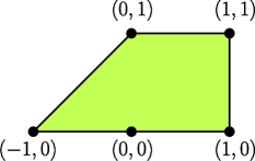
Figure 8: Suspended pinch point

In this section, we allow $P$ to be simply a set of integral vectors of a form $(*,*,1)$, not necessarily the vertices (extremal points) of a convex polygon. Such $P$ will be referred to as a generalized toric diagram; the set of generalized toric diagrams will be denoted by ${\mathcal{T}_{\mathrm{gen}}}$. The definitions of the zonotope $Z_{P}(\phi)$, the function $F_{P}=\mathop{\rm vol}({\mathcal{Z}}_{P}(\phi))$ and $\mathfrak{M}(P)$ goes through without any change for any $P\in{\mathcal{T}_{\mathrm{gen}}}$; we agree that the coefficient $c_{ijk}$ is always given by $|\det(\bm{v}_{i},\bm{v}_{j},\bm{v}_{k})|$ even if the triangle $\triangle(\bm{v}_{i},\bm{v}_{j},\bm{v}_{k})$ has negative orientation or contain other $\bm{v}_{l}$ inside.

The next Proposition shows that if a non-extremal point $\bm{v}_{p}$ exists, the maximization process drives us to the boundary $\phi^{p}=0$. Therefore, as far as the maximization of $F_{P}$ is concerned, the non-extremal points are safely ignored. In physical terms, the corresponding global symmetry “decouples” as a result of $a$-maximization.

Proposition 8.1

Let $P=\{\bm{v}_{1},\dots,\bm{v}_{n}\}\in{\mathcal{T}_{\mathrm{gen}}}$ be a generalized toric diagram. Suppose $\bm{v}_{p}$ is not an extremal point of the convex hull of $P$. Then the volume $F_{P}:\Gamma_{n}\to{\mathbb{R}}$ attains its maximum on the boundary $\partial\Gamma_{n}$ corresponding to the hyperplane $\phi^{p}=0$. In other words, if we put $P^{\prime}:=P\setminus\{\bm{v}_{p}\}=\{\bm{v}_{1},\dots,\bm{v}_{p-1},\bm{v}_{p+1},\dots,\bm{v}_{n}\}\in{\mathcal{T}_{\mathrm{gen}}}$, then

$$\max_{\phi\in\Gamma_{n}}F_{P}(\phi)=\max_{\phi^{\prime}\in\Gamma_{n-1}}F_{P^{\prime}}(\phi^{\prime}).$$

Corollary 8.2

For any $P\in{\mathcal{T}_{\mathrm{gen}}}$, the maximum values of $F_{P}$ is solely determined by the convex hull of $P$; if $P$ and $Q$ are two generalized toric diagrams such that $\mathop{\rm conv}(P)=\mathop{\rm conv}(Q)$, then $\mathfrak{M}(P)=\mathfrak{M}(Q)$.

Proof. (of Proposition 8.1)

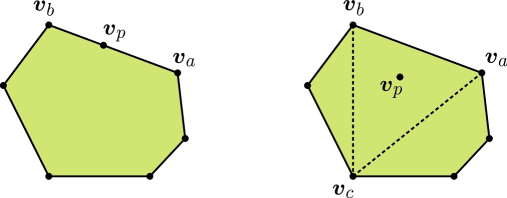
Figure 9: Left, case (i): $\bm{v}_{p}=\alpha\bm{v}_{a}+\beta\bm{v}_{b}$. Right, case (ii) : $\bm{v}_{p}=\alpha\bm{v}_{a}+\beta\bm{v}_{b}+\gamma\bm{v}_{c}$.

There are two cases to be handled: (i) $\bm{v}_{p}\in\partial P$ and (ii) $\bm{v}_{p}\in\mathop{\rm relint}(P)$ (Figure 9).

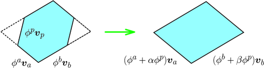
Figure 10: Elimination of the non-extremal vector $\bm{v}_{p}=\alpha\bm{v}_{a}+\beta\bm{v}_{b}$.

Consider the case (i) first. Let us assume $\bm{v}_{p}$ is on a edge $\mathop{\rm relint}(\mathop{\rm conv}(\bm{v}_{a},\bm{v}_{b}))$; put $\bm{v}_{p}=\alpha\bm{v}_{a}+\beta\bm{v}_{b}$ for some $\alpha,\beta>0$, $\alpha+\beta=1$. Suppose that, contrary to our claim, the maximum of $F_{P}$ is attained at $\phi=(\phi^{1},\dots,\phi^{p},\dots,\phi^{n})$ with $\phi^{p}>0$. Then we have a following proper inclusion (Figure 10):

$$\phi^{a}[\bm{0},\bm{v}_{a}]+\phi^{b}[\bm{0},\bm{v}_{b}]+\phi^{p}[\bm{0},\bm{v}_{p}]=\phi^{a}[\bm{0},\bm{v}_{a}]+\phi^{b}[\bm{0},\bm{v}_{b}]+\phi^{p}[\bm{0},\alpha\bm{v}_{a}+\beta\bm{v}_{b}]$$

$$\qquad\qquad\subsetneq(\phi^{a}+\alpha\phi^{p})[\bm{0},\bm{v}_{a}]+(\phi^{b}+\beta\phi^{p})[\bm{0},\bm{v}_{b}].$$ (20)

Adding $\sum_{i\neq a,b,p}\phi^{i}[\bm{0},\bm{v}_{i}]$ to both sides of (20), we have ${\mathcal{Z}}_{P}(\phi)\subsetneq{\mathcal{Z}}_{P}(\phi_{\bullet})$, where the point $\phi_{\bullet}\in\partial\Gamma_{n}$ is defined by

$$\phi_{\bullet}^{i}=\left\{\begin{array}[]{ll}\phi^{a}+\alpha\phi^{p},&\mbox{if $i=a$},\\ \phi^{b}+\beta\phi^{p},&\mbox{if $i=b$},\\ 0,&\mbox{if $i=p$},\\ \phi^{i},&\mbox{otherwise}.\end{array}\right.$$

Thus we have $F_{P}(\phi)=\mathop{\rm vol}({\mathcal{Z}}_{P}(\phi))<\mathop{\rm vol}({\mathcal{Z}}_{P}(\phi_{\bullet}))=F_{P}(\phi_{\bullet})$. More explicitly,

$$F_{P}(\phi_{\bullet})-F_{P}(\phi)=\alpha\beta\sum_{i\neq a,b,p}|\det(\bm{v}_{a},\bm{v}_{b},\bm{v}_{i})|\phi^{a}\phi^{b}\phi^{i}>0.$$

This contradicts the assumption that $\phi$ is a maximum point.

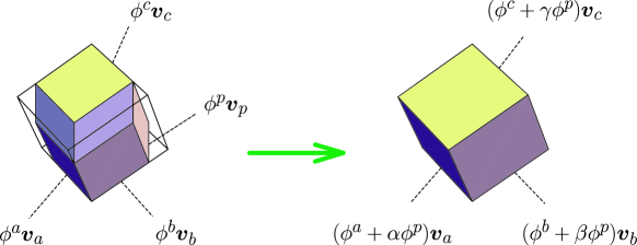
Figure 11: Elimination of the non-extremal vector $\bm{v}_{p}=\alpha\bm{v}_{a}+\beta\bm{v}_{b}+\gamma\bm{v}_{c}$

The case (ii) is similar. There exist three vertices $\bm{v}_{a},\bm{v}_{b},\bm{v}_{c}$ ($a,b,c\neq p$) such that $\bm{v}_{p}\in\mathop{\rm conv}(\bm{v}_{a},\bm{v}_{b},\bm{v}_{c})$. Let $\alpha,\beta,\gamma$ be three nonnegative numbers such that $\alpha+\beta+\gamma=1$ and $\bm{v}_{p}=\alpha\bm{v}_{a}+\beta\bm{v}_{b}+\gamma\bm{v}_{c}$. To obtain a contradiction, suppose that $F_{P}$ takes its maximum at $\phi=(\phi^{1},\dots,\phi^{p},\dots,\phi^{n})\in\Gamma_{n}$ with $\phi^{p}>0$. We have a following proper inclusion (Figure 11)

$$\phi^{a}[\bm{0},\bm{v}_{a}]+\phi^{b}[\bm{0},\bm{v}_{b}]+\phi^{c}[\bm{0},\bm{v}_{c}]+\phi^{p}[\bm{0},\bm{v}_{p}]$$

$$=\phi^{a}[\bm{0},\bm{v}_{a}]+\phi^{b}[\bm{0},\bm{v}_{b}]+\phi^{c}[\bm{0},\bm{v}_{c}]+\phi^{p}[\bm{0},\alpha\bm{v}_{a}+\beta\bm{v}_{b}+\phi^{c}\bm{v}_{c}]$$

$$\subsetneq(\phi^{a}+\alpha\phi^{p})[\bm{0},\bm{v}_{a}]+(\phi^{b}+\beta\phi^{p})[\bm{0},\bm{v}_{b}]+(\phi^{a}+\gamma\phi^{c})[\bm{0},\phi^{c}\bm{v}_{c}].$$ (21)

Adding $\sum_{i\neq a,b,c,p}\phi^{i}[\bm{0},\bm{v}_{i}]$ to both sides of (21), we have ${\mathcal{Z}}_{P}(\phi)\subsetneq{\mathcal{Z}}_{P}(\phi_{\bullet})$ where the point $\phi_{\bullet}\in\partial\Gamma_{n}$ is defined by

$$\phi_{\bullet}^{i}=\left\{\begin{array}[]{ll}\phi^{a}+\alpha\phi^{p},&\mbox{if $i=a$},\\ \phi^{b}+\beta\phi^{p},&\mbox{if $i=b$},\\ \phi^{c}+\gamma\phi^{p},&\mbox{if $i=c$},\\ 0,&\mbox{if $i=p$},\\ \phi^{i},&\mbox{otherwise}.\end{array}\right.$$

Thus we have $F_{P}(\phi)=\mathop{\rm vol}({\mathcal{Z}}_{P}(\phi))<\mathop{\rm vol}({\mathcal{Z}}_{P}(\phi_{\bullet}))=F_{P}(\phi_{\bullet})$. More explicitly, the volume increases by

$$F_{P}(\phi_{\bullet})-F_{P}(\phi) = \alpha\beta\gamma\;|\det(\bm{v}_{a},\bm{v}_{b},\bm{v}_{c})|\phi^{a}\phi^{b}\phi^{c}+\alpha\beta\sum_{i\neq a,b,p}|\det(\bm{v}_{a},\bm{v}_{b},\bm{v}_{i})|\phi^{a}\phi^{b}\phi^{i}$$

$$+\beta\gamma\sum_{i\neq b,c,p}|\det(\bm{v}_{b},\bm{v}_{c},\bm{v}_{i})|\phi^{b}\phi^{c}\phi^{i}+\gamma\alpha\sum_{i\neq c,a,p}|\det(\bm{v}_{c},\bm{v}_{a},\bm{v}_{i})|\phi^{c}\phi^{a}\phi^{i}>0.$$

This is a contradiction. $\Box$

We investigate a few more ways of changing toric diagrams.

Proposition 8.3

Suppose a toric diagram $P$ is obtained from a toric diagram $Q$ by elongating one or two edges of $Q$ as in Figure 12. Then, $\mathfrak{M}(Q)<\mathfrak{M}(P).$

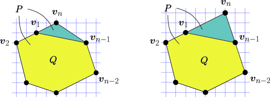
Figure 12: Elongating one or two edges of a toric diagram

Proof. Consider the toric diagram $P$ in Figure 12 on the left. $\bm{v}_{1}$ is non-extremal point of $P$, thus

$$\mathfrak{M}(P) = \mathfrak{M}(\{\bm{v}_{2},\dots,\bm{v}_{n-1},\bm{v}_{n}\})$$

$$= \mathfrak{M}(\{\bm{v}_{1},\bm{v}_{2},\dots,\bm{v}_{n-1},\bm{v}_{n}\})\qquad\mbox{by Corollary \ref{cor:OnlyVerticesMatter} }$$

$$> \mathfrak{M}(\{\bm{v}_{1},\bm{v}_{2},\dots,\bm{v}_{n-1}\})\qquad~{}~{}~{}~{}~{}\mbox{by Corollary \ref{cor:Monotonicity} }$$

$$= \mathfrak{M}(Q).$$

The toric diagrams on the right of Figure 12 can be handled in much the same way. $\Box$

Proposition 8.4

Suppose a toric diagram $P$ is obtained from a toric diagram $Q$ by pushing out one vertex of $Q$ as depicted in Figure 13 on the left. Then, $\mathfrak{M}(Q)<\mathfrak{M}(P)$.

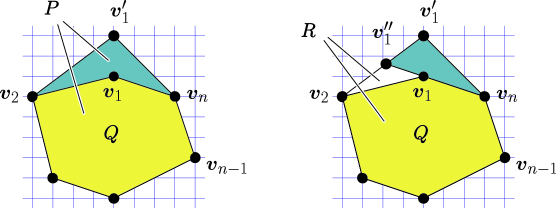
Figure 13: Pushing out a vertex of a toric diagram

Proof. Label the vertices of $P$ and $Q$ as in Figure 13. Construct another polygon $R=\{\bm{v}^{\prime\prime}_{1},\bm{v}_{2},\dots$ $,\bm{v}_{n-1},\bm{v}_{n}\}$ by extending the edge $(\bm{v}_{n},\bm{v}_{1})$ into the direction of $\bm{v}_{1}$ until it touches the edge $(\bm{v}^{\prime}_{1},\bm{v}_{2})$ at $\bm{v}^{\prime\prime}_{1}$ (Figure 13, right). Clearly $Q\subsetneq R\subsetneq P$. Applying Proposition 8.3 twice, we have $\mathfrak{M}(Q)<\mathfrak{M}(R)<\mathfrak{M}(P)$. $\Box$

Now suppose $P$ and $P^{\prime}$ are two toric diagrams satisfying $P\subset P^{\prime}$. It is clear that there is a sequence of toric diagrams (or rational polygons)

$$P=Q_{0}\subset Q_{1}\subset Q_{2}\subset\dots\subset Q_{k-1}\subset Q_{k}=P^{\prime}$$ (22)

such that $Q_{i}$ ($1\leq i\leq k$) is obtained from $Q_{i-1}$, either

• by adding an extra vertex to $Q_{i-1}$ (Proposition 6.1),

• by elongating one or two edges of $Q_{i-1}$ (Proposition 8.3), or

• by pushing out one vertex of $Q_{i-1}$ (Proposition 8.4).

In either case, we know that $\mathfrak{M}(Q_{i-1})<\mathfrak{M}(Q_{i})$. Consequently, we have demonstrated the following monotone property of the maximum value of $F_{P}$, or modulus $\mathfrak{M}(P)$, with respect to the change of the toric diagrams:

Theorem 8.5

Let $P$ and $P^{\prime}$ be two toric diagrams satisfying $[P]\preceq[P^{\prime}]$, where $\preceq$ is the partial order defined in (8). Then $\mathfrak{M}(P)\leq\mathfrak{M}(P^{\prime})$. The equality holds if and only if $P\simeq P^{\prime}$, i.e. equal up to integral affine transformations on ${\mathbb{Z}}^{2}$.

9 Relation to volume minimization

In the preceding sections we have concerned ourselves with the extremization of homogeneous polynomial $\hat{F}_{P}:{\mathbb{R}}_{\geq 0}^{n}\to{\mathbb{R}}$ under the constraint

$$\rho(\phi)=\phi^{1}+\dots+\phi^{n}=r.$$ (23)

Now consider a following variant of the extremization problem.

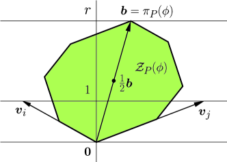
Figure 14: Zonotope and Reeb vector $\bm{b}$

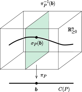
Figure 15: Fibration $\pi_{P}:{\mathbb{R}}_{\geq 0}^{n}\to C(P)$ and fiberwise critical point $\sigma_{P}(\bm{b})$.

As before, let $P\in{\mathcal{T}}$ be a toric diagram and $\bm{v}_{1},\dots,\bm{v}_{n}$ be its vertices in counterclockwise order. Define a map $\pi_{P}:{\mathbb{R}}_{\geq 0}^{n}\to{\mathbb{R}}^{3}$ by

$$\pi_{P}(\phi)=\sum_{i=1}^{n}\phi^{i}\bm{v}_{i}.$$

The image of $\pi_{P}$ is the cone $C(P)$ over the toric diagram $P$ (Figure 1). In terms of the zonotope ${\mathcal{Z}}_{P}(\phi)$, $\bm{b}=\pi_{P}(\phi)$ is the location of the vertex opposite to the origin $\bm{0}$, and $\frac{1}{2}\bm{b}$ is the center (Figure 15). As we will see, $\bm{b}\in C(P)$ can be identified with the Reeb vector of a Sasaki-Einstein manifold.

Due to the fact that each $\bm{v}_{i}$ is of the form $(*,*,1)$, the constraint (23) factors through the projection $\pi_{P}$:

$$\begin{array}[]{ccccccc}\rho&:&{\mathbb{R}}_{\geq 0}^{n}&\stackrel{{\scriptstyle\pi_{P}}}{{\longrightarrow}}&C(P)&\stackrel{{\scriptstyle h}}{{\longrightarrow}}&{\mathbb{R}}\\ &&\cup&&\cup&&\cup\\ &&\Gamma_{n}&\stackrel{{\scriptstyle\pi_{P}}}{{\longrightarrow}}&rP&\stackrel{{\scriptstyle h}}{{\longrightarrow}}&\{r\}\\ \end{array}$$

where $h(x,y,z)=z$. The image of $\Gamma_{n}$ under $\pi_{P}$ is $rP=h^{-1}(r)$, namely the horizontal slice of the cone $C(P)$ at height $r$.

For a generic $\bm{b}\in C(P)$, the fiber $\pi_{P}^{-1}(\bm{b})$ of the projection $\pi_{P}:{\mathbb{R}}_{\geq 0}^{n}\to C(P)$ is an $(n{-}3)$-dimensional convex polytope. This fibration structure allows us to extremize $F_{P}:\Gamma_{n}\to{\mathbb{R}}$ in two steps: first in the fiber direction, and then in the base direction (Figure 15):

$$\max_{\phi\in\Gamma_{n}}\hat{F}_{P}(\phi)=\max_{\bm{b}\in rP}\biggl{\{}\max_{\phi\in\pi_{P}^{-1}(\bm{b})}\hat{F}_{P}(\phi)\biggr{\}}.$$

The following theorem shows the maximization along the fiber direction is rather straightforward and admits an explicit solution.

Theorem 9.1

Let $r>0$ and $\bm{b}$ be a point in $rP\subset C(P)$.

• The restriction $\hat{F}_{P}|_{\pi_{P}^{-1}(\bm{b})}$ of $\hat{F}_{P}$ along the fiber $\pi_{P}^{-1}(\bm{b})$ is a quadratic polynomial.

• The quadratic polynomial $\hat{F}_{P}|_{\pi_{P}^{-1}(\bm{b})}$ has a unique critical point $\sigma_{P}(\bm{b})$ and it is also a maximum. The point $\sigma_{P}(\bm{b})$ is determined as follows: Let $\ell_{P}:{\mathbb{R}}^{3}\to{\mathbb{R}}^{n}$ be a vector-valued rational function defined by

  $$\ell_{P}^{i}(\bm{b}):=\frac{\left\langle\bm{v}_{i-1},\bm{v}_{i},\bm{v}_{i+1}\right\rangle}{\left\langle\bm{b},\bm{v}_{i-1},\bm{v}_{i}\right\rangle\left\langle\bm{b},\bm{v}_{i},\bm{v}_{i+1}\right\rangle},\qquad(\bm{b}\in{\mathbb{R}}^{3},~{}~{}i=1,\dots,n).$$

  Then

  $$\sigma_{P}^{i}(\bm{b})=\frac{r}{V_{P}(\bm{b})}\ell_{P}^{i}(\bm{b}),\qquad(i=1,\dots,n)$$ (24)

  where

  $$V_{P}(\bm{b}):=\sum_{i=1}^{n}\ell_{P}^{i}(\bm{b}).$$

  The critical value is given by

  $$\max_{\phi\in\pi_{P}^{-1}(\bm{b})}\hat{F}_{P}(\phi)=\hat{F}_{P}(\sigma_{P}(\bm{b}))=\frac{r}{V_{P}(\bm{b})}.$$

Before we turn to the proof of Theorem 9.1, it is useful to take a small detour into the AdS/CFT correspondence and the volume minimization.

The AdS/CFT-correspondence [22, 23, 24, 25] has brought a novel insight into the relation between $N{=}1$ SCFT and Sasaki-Einstein manifolds. The world-volume theory on the D3 branes living at conical Calabi-Yau singularities is dual to a type IIB background of the form $AdS_{5}\times Y$, where $Y$ is the five dimensional horizon manifold [26, 27, 28]. Supersymmetry requires that $Y$ is a Sasaki-Einstein manifold and the cone $X=C(Y)$ over the base $Y$ is a Calabi-Yau threefold with Gorenstein singularity.

If $Y$ is toric, i.e. its isometry group contains at least three torus, then $X$ is a toric Calabi-Yau singularity. It is known [29] that every toric Gorenstein Calabi-Yau singularity is obtained as a toric variety $X_{P}$ associated with a fan $C(P)$, the cone over a toric diagram $P$. The toric variety $X_{P}$ is equipped with a moment map $\mu:X_{P}\to{\mathbb{R}}^{3}$ associated with the $T^{3}\subset({\mathbb{C}}^{*})^{3}$ action. The image of $\mu$ is the dual cone $C(P)^{\vee}$, and the generic fiber of $\mu$ is $T^{3}$. The corresponding Sasaki-Einstein manifold $Y_{P}$ has a canonically defined constant norm Killing vector field, called Reeb vector field; it is identified with a vector $\bm{b}$ in $C(P)$ via moment map $\mu$. Each vertex $\bm{v}_{i}$ of $P$ determines a toric divisor $D_{i}$ in $X_{P}$, which is a cone over a certain calibrated three dimensional submanifold $\Sigma_{i}$ in $Y_{P}$.

The Calabi-Yau cone $X_{P}$ can be also constructed as a symplectic quotient [30, 31, 32] (up to some finite abelian group)

$$X_{P}\simeq{\mathbb{C}}^{n}//({\mathbb{C}}^{*})^{n-3}.$$ (25)

The standard $({\mathbb{C}}^{*})^{n}$ action on ${\mathbb{C}}^{n}$ can be decomposed into $({\mathbb{C}}^{*})^{n-3}$ and $({\mathbb{C}}^{*})^{3}$ corresponding to the exact sequence

$$0\longrightarrow{\mathbb{R}}^{n-3}\longrightarrow{\mathbb{R}}^{n}\stackrel{{\scriptstyle\pi_{P}}}{{\longrightarrow}}{\mathbb{R}}^{3}\longrightarrow 0.$$

The $({\mathbb{C}}^{*})^{n-3}$ action, defining the quotient action in (25), is called baryonic symmetries in physics literature; $({\mathbb{C}}^{*})^{3}$ acting nontrivially on $X_{P}$ is referred to as flavor symmetries. The flavor (resp. baryonic) symmetry corresponds to the base (resp. fiber) direction of the fibration $\pi_{P}:{\mathbb{R}}_{\geq 0}^{n}\to C(P)$.

According to the prediction of AdS/CFT correspondence, the central charge $a$ of the SCFT and the volume of the internal manifold are related as [33, 34]

$$a=\frac{N^{2}\pi^{3}}{4\mathop{\rm vol}(Y)},$$

while the exact $R$-charges of chiral fields are proportional to the volumes of three cycles $\Sigma_{i}\subset Y_{P}$ [35]

$$R_{i}=\frac{\pi}{3}\frac{\mathop{\rm vol}(\Sigma_{i})}{\mathop{\rm vol}(Y)}.$$

It is usually quite difficult to obtain Einstein metrics explicitly; it thus appears impossible to compute these volumes. Remarkably, Martelli, Sparks and Yau [10, 11] proved that the volumes of $Y_{P}$ and $\Sigma_{i}$’s can be computed without actually knowing the metric, provided the Reeb vector $\bm{b}\in 3P$ is known for the Calabi-Yau cone:

$$\mathop{\rm vol}(\Sigma_{i}) = {2\pi^{2}}\ell_{P}^{i}(\bm{b}),$$

$$\mathop{\rm vol}(Y_{P}) = \frac{\pi}{6}\sum_{i=1}^{n}\mathop{\rm vol}(\Sigma_{i})=\frac{\pi^{3}}{3}V_{P}(\bm{b}).$$

Here, the functions $\ell_{P}^{i}(\bm{b})$ and $V_{P}(\bm{b})$ of $\bm{b}$ are nothing but those defined in Theorem 9.1. Even more importantly, these authors showed that the correct Reeb vector is characterized as the vector $\bm{b}\in 3P$ which minimize the “trial volume function” $V_{P}(\bm{b})$. This is a beautiful geometrical counterpart of the $a$-maximization.

It should be clear now how the volume minimization and “$a$-maximization in two steps” are related. Theorem 9.1 can be summarized as the following

Theorem 9.2

(i) For $\bm{b}=(*,*,r)\in\mathop{\rm relint}(rP)$, the trial volume function $V_{P}(\bm{b})$ is inversely proportional to the maximum of the $a$-function in the fiber $\pi_{P}^{-1}(\bm{b})$:

$$\max_{\phi\in\pi_{P}^{-1}(\bm{b})}F_{P}(\phi)=\frac{r}{V_{P}(\bm{b})}.$$

(ii) The $a$-maximization and the volume minimization are equivalent in the sense that

$$\max_{\phi\in\rho^{-1}(r)}F_{P}(\phi)=\frac{r}{\displaystyle\min_{\bm{b}\in\mathop{\rm relint}(rP)}V_{P}(\bm{b})}.$$

Theorem 9.2 is essentially due to Butti-Zaffaroni [12]. Our approach has an advantage that the existence of the maximum in each fiber is almost immediate from the concavity.

Let us now turn to the proof of Theorem 9.1. We first prove the following

Lemma 9.3

$$\hat{F}_{P}(\phi)=\biggl{(}\sum_{i=1}^{n}\phi^{i}\bm{v}_{i}\biggr{)}\cdot\biggl{(}\sum_{1\leq j<k\leq n}^{n}\phi^{j}\phi^{k}\bm{v}_{j}\times\bm{v}_{k}\biggr{)}.$$

Proof. The right hand side can be rewritten as follows:

$$\sum_{i=1}^{n}\sum_{1\leq j<k\leq n}^{n}\phi^{i}\phi^{j}\phi^{k}\left\langle\bm{v}_{i},\bm{v}_{j},\bm{v}_{k}\right\rangle$$

$$= \biggl{(}\sum_{1\leq i<j<k\leq n}^{n}+\sum_{1\leq j<i<k\leq n}^{n}+\sum_{1\leq j<k<i\leq n}^{n}\biggr{)}\phi^{i}\phi^{j}\phi^{k}\left\langle\bm{v}_{i},\bm{v}_{j},\bm{v}_{k}\right\rangle$$

$$= \sum_{1\leq i<j<k\leq n}^{n}\phi^{i}\phi^{j}\phi^{k}\bigl{(}\left\langle\bm{v}_{i},\bm{v}_{j},\bm{v}_{k}\right\rangle+\left\langle\bm{v}_{j},\bm{v}_{i},\bm{v}_{k}\right\rangle+\left\langle\bm{v}_{k},\bm{v}_{i},\bm{v}_{j}\right\rangle\bigr{)}$$

$$= \sum_{1\leq i<j<k\leq n}^{n}\phi^{i}\phi^{j}\phi^{k}\bigl{(}\left\langle\bm{v}_{i},\bm{v}_{j},\bm{v}_{k}\right\rangle-\left\langle\bm{v}_{i},\bm{v}_{j},\bm{v}_{k}\right\rangle+\left\langle\bm{v}_{i},\bm{v}_{j},\bm{v}_{k}\right\rangle\bigr{)}$$

$$= \sum_{1\leq i<j<k\leq n}^{n}\phi^{i}\phi^{j}\phi^{k}\left\langle\bm{v}_{i},\bm{v}_{j},\bm{v}_{k}\right\rangle=\hat{F}_{P}(\phi).$$

$\Box$

The first claim of Theorem 9.1 follows immediately from Lemma 9.3; the restriction of $\hat{F}_{P}$ to the fiber $\pi_{P}^{-1}(\bm{b})$ equals a quadratic polynomial

$$Q(\phi):=\sum_{1\leq j<k\leq n}^{n}\left\langle\bm{b},\bm{v}_{j},\bm{v}_{k}\right\rangle\phi^{j}\phi^{k},\qquad(\phi\in\pi_{P}^{-1}(\bm{b})).$$

To compute the critical point of $Q$, introduce an $n\times n$ symmetric matrix $A=(A_{ij})$ defined by

$$A_{ij}=A_{ji}=\frac{1}{2}\left\langle\bm{b},\bm{v}_{i},\bm{v}_{j}\right\rangle,\qquad(1\leq i\leq j\leq n)$$

so that $Q(\phi)=\sum_{i,j=1}^{n}A_{ij}\phi^{i}\phi^{j}$.

The extremization of $Q:\pi_{P}^{-1}(\bm{b})\to{\mathbb{R}}$ is equivalent to that of a function $\tilde{Q}$ defined by

$$\tilde{Q}=\sum_{i,j=1}^{n}A_{ij}\phi^{i}\phi^{j}-\bm{\lambda}\cdot\bigl{(}\sum_{i=1}^{n}\phi^{i}\bm{v}_{i}-\bm{b}\bigr{)}$$

where $\bm{\lambda}\in{\mathbb{R}}^{3}$ is the Lagrange multiplier imposing the constraint $\pi_{P}(\phi)=\bm{b}$. The equation $d\tilde{Q}=0$ gives

$$2\sum_{j=1}^{n}A_{ij}\sigma_{P}(\bm{b})^{j}-\bm{\lambda}\cdot\bm{v}_{i}=0,\qquad(i=1,\dots,n)$$ (26)

or equivalently,

$$\sigma_{P}(\bm{b})^{i}=\frac{1}{2}\sum_{j=1}^{n}(A^{-1})^{ij}\bm{\lambda}\cdot\bm{v}_{j}.\qquad(i=1,\dots,n)$$ (27)

In Appendix, the inverse matrix $A^{-1}$, which exists if $\bm{b}\in\mathop{\rm relint}(C(P))$, is explicitly calculated. Applying Proposition A.1 (i) to (27), we have

$$\sigma_{P}(\bm{b})^{i} = \frac{1}{2}\biggl{[}(A^{-1})^{i\,i{-}1}\bm{\lambda}\cdot\bm{v}_{i-1}+(A^{-1})^{i\,i}\bm{\lambda}\cdot\bm{v}_{i}+(A^{-1})^{i\,i{+}1}\bm{\lambda}\cdot\bm{v}_{i+1}\biggr{]}$$ (28)

$$= \frac{1}{2}\frac{\left\langle\bm{v}_{i-1},\bm{v}_{i},\bm{v}_{i+1}\right\rangle}{\left\langle\bm{b},\bm{v}_{i-1},\bm{v}_{i}\right\rangle\left\langle\bm{b},\bm{v}_{i},\bm{v}_{i+1}\right\rangle}\bm{\lambda}\cdot\bm{b}$$

$$= \frac{1}{2}(\bm{\lambda}\cdot\bm{b})\;\ell_{P}^{i}(\bm{b}),\qquad(i=1,\dots,n).$$

Summing over $i$ and using the constraint $r=\sum_{i=1}^{n}\sigma_{P}(\bm{b})^{i}$, one has

$$\frac{1}{2}(\bm{\lambda}\cdot\bm{b})=\frac{r}{\sum_{i=1}^{n}\ell_{P}^{i}(\bm{b})}=\frac{r}{V_{P}(\bm{b})}.$$ (29)

The formula (24) follows from (28) and (29). The critical value is then given by, from (26) and (29),

$$Q(\sigma_{P}(\bm{b})) = \sum_{i,j=1}^{n}\sigma_{P}(\bm{b})^{i}(A_{ij}\sigma_{P}(\bm{b})^{j})=\frac{1}{2}\sum_{i=1}^{n}\sigma_{P}(\bm{b})^{i}(\bm{\lambda}\cdot\bm{v}_{i})$$

$$= \frac{1}{2}\bm{\lambda}\cdot\pi_{P}(\sigma_{P}(\bm{b}))=\frac{1}{2}\bm{\lambda}\cdot\bm{b}=\frac{r}{V_{P}(\bm{b})}.$$

The critical point $\sigma(\bm{b})$ of $Q$ is easily seen to be a maximum along the similar lines as the proof of Proposition 5.5. This completes the proof of Theorem 9.1.

10 Summary and outlook

In this paper, we proved that for any toric diagram $P$, the $a$-maximization always leads to the unique solution, which satisfies a universal upper bound. A combinatorial analogue of $a$-theorem is also established: the $a$-function always decreases when a toric diagram gets smaller. The relation between $a$-maximization and volume minimization is also discussed.

A tacit assumption in this paper is that a quiver gauge theory is uniquely determined by a toric diagram. The formulae (5) and (6) are associated with toric diagrams so naturally that there seems to be no other choice. However, the brane-tiling technique [36, 15] allows us to produce many examples of gauge theories whose matter content is different from what we studied in this paper; they are regarded as realizing different “phases” of the same SCFT. The gauge theory studied in this paper is called “minimal” in [12]; conjecturally the number of chiral fields given in (2) is smaller than that of any other possible phases. It is interesting to study $a$-maximization of those non-minimal phases and compare with the minimal ones.

Since the polynomial $F_{P}$ is defined over the integers, the maximum value of $F_{P}$ or $\mathfrak{M}(P)$ is always an algebraic number. Does this critical value characterize SCFT uniquely? In two dimensions, there are examples of non-isomorphic CFTs with equal Virasoro central charges. The situation is not clear for higher dimensions. As we have seen, the $a$-maximization defines a natural map

$$\mathfrak{M}\;:\;{\mathcal{T}}/\simeq\quad\longrightarrow\quad\overline{{\mathbb{Q}}}\cap{\mathbb{R}}_{\geq 0}.$$

Theorem 8.5 asserts that $\mathfrak{M}$ is strictly decreasing along any descending chain (totally ordered subset) of ${\mathcal{T}}/\simeq$. Although $\mathrm{Area}(P)$ shares this property, they just encode the number of gauge fields; there are many toric diagrams of the same area but different modulus. It seems that modulus $\mathfrak{M}$ is far more sensitive to the shape of toric diagrams than the area. We conjecture that the map $\mathfrak{M}$ is injective.

Probably the most important question is why zonotopes come into play in $a$-maximization. We believe that a deeper understanding of this will shed new light on the AdS/CFT correspondence.

Appendix A Appendix: A symmetric matrix and its inverse

Proposition A.1

Let $\bm{b},\bm{v}_{1},\dots,\bm{v}_{n}$ be vectors in ${\mathbb{R}}^{3}$ and $A=(A_{ij})$ be an $n\times n$ symmetric matrix given by

$$A_{ij}=A_{ji}=\frac{1}{2}\left\langle\bm{b},\bm{v}_{i},\bm{v}_{j}\right\rangle,\qquad(1\leq i\leq j\leq n).$$

Define an $n\times n$ symmetric ‘almost tridiagonal’ matrix $B=(B_{ij})$ by

$$B_{ij}=B_{ji}=\left\{\begin{array}[]{ll}\displaystyle-\frac{\left\langle\bm{b},\bm{v}_{i-1},\bm{v}_{i+1}\right\rangle}{\left\langle\bm{b},\bm{v}_{i-1},\bm{v}_{i}\right\rangle\left\langle\bm{b},\bm{v}_{i},\bm{v}_{i+1}\right\rangle},&\mbox{if $j=i$},\\[8.61108pt] \displaystyle\frac{1}{\left\langle\bm{b},\bm{v}_{i},\bm{v}_{i+1}\right\rangle},&\mbox{if $j=i+1$},\\[8.61108pt] \displaystyle\frac{1}{\left\langle\bm{b},\bm{v}_{1},\bm{v}_{n}\right\rangle},&\mbox{if $i=1$ and $j=n$},\\[8.61108pt] 0,&\mbox{otherwise},\end{array}\right.$$

for $1\leq i\leq j\leq n$. Here $\bm{v}_{0}:=\bm{v}_{n}$ and $\bm{v}_{n+1}:=\bm{v}_{1}$.

• For $1\leq i\leq n$,

  $$B_{i,i-1}\bm{v}_{i-1}+B_{i,i}\bm{v}_{i}+B_{i,i+1}\bm{v}_{i+1}=\frac{\left\langle\bm{v}_{i-1},\bm{v}_{i},\bm{v}_{i+1}\right\rangle}{\left\langle\bm{b},\bm{v}_{i-1},\bm{v}_{i}\right\rangle\left\langle\bm{b},\bm{v}_{i},\bm{v}_{i+1}\right\rangle}\bm{b}.$$ (30)

  Here we assume $B_{1,0}:=-B_{1,n}$ and $B_{n,n+1}:=-B_{n,1}$.

• The matrices $A$ and $B$ are inverse to each other.

Proof. (i)  Suppose for a moment that $\bm{v}_{i-1},\bm{v}_{i},\bm{v}_{i+1}$ are linearly independent. Expanding $\bm{b}$ as $\bm{b}=\alpha\bm{v}_{i-1}+\beta\bm{v}_{i}+\gamma\bm{v}_{i+1}$, it is easy to check that the both sides of (30) are equal to

$$\frac{1}{\alpha\gamma\left\langle\bm{v}_{i-1},\bm{v}_{i},\bm{v}_{i+1}\right\rangle}(\alpha\bm{v}_{i-1}+\beta\bm{v}_{i}+\gamma\bm{v}_{i+1}).$$

Since (30) is an equality of a rational functions of $\bm{v}_{i}$’s and $\bm{b}$, (30) is true in general by the continuity argument.

(ii)  It suffices to verify $BA=I$, entry by entry. For $1\leq i<j\leq n$,

$$(BA)_{i,j} = B_{i,i{-}1}A_{i{-}1,j}+B_{i,i}A_{i,j}+B_{i,i{+}1}A_{i{+}1,j}$$

$$= \frac{1}{2}B_{i,i{-}1}\left\langle\bm{b},\bm{v}_{i-1},\bm{v}_{j}\right\rangle+\frac{1}{2}B_{i,i}\left\langle\bm{b},\bm{v}_{i},\bm{v}_{j}\right\rangle+\frac{1}{2}B_{i,i{+}1}\left\langle\bm{b},\bm{v}_{i+1},\bm{v}_{j}\right\rangle$$

$$= \frac{1}{2}\left\langle\bm{b},(B_{i,i-1}\bm{v}_{i-1}+B_{i,i}\bm{v}_{i}+B_{i,i+1}\bm{v}_{i+1}),\bm{v}_{j}\right\rangle,$$

which vanishes by (30). Similarly $(BA)_{ij}=0$ for $1\leq j<i\leq n$. On the other hand, for $1<i<n$,

$$(BA)_{i,i} = B_{i,i{-}1}A_{i{-}1,i}+B_{i,i{+}1}A_{i{+}1,i}$$

$$= B_{i{-}1,i}A_{i{-}1,i}+B_{i,i{+}1}A_{i,i{+}1}$$

$$= \frac{1}{\left\langle\bm{b},\bm{v}_{i-1},\bm{v}_{i}\right\rangle}\cdot\frac{1}{2}\left\langle\bm{b},\bm{v}_{i-1},\bm{v}_{i}\right\rangle+\frac{1}{\left\langle\bm{b},\bm{v}_{i},\bm{v}_{i+1}\right\rangle}\cdot\frac{1}{2}\left\langle\bm{b},\bm{v}_{i+1},\bm{v}_{i}\right\rangle$$

$$= \frac{1}{2}+\frac{1}{2}=1.$$

With extra care for signs, the cases of $i=1,n$ are similarly verified. $\Box$

References

[1]
A. B. Zomolodchikov, “Irreversibility” of the flux of the
renormalization group in a D field theory, Pis′ma Zh.
Èksper. Teoret. Fiz.43 (1986), no. 12 565–567.
[2]
M. J. Duff, Twenty years of the Weyl anomaly, Class. Quant.
Grav.11 (1994) 1387–1404,
[hep-th/9308075].
[3]
J. L. Cardy, Is there a -theorem in four dimensions?, Phys.
Lett. B215 (1988), no. 4 749–752.
[4]
V. K. Dobrev and V. B. Petkova, All positive energy unitary irreducible
representations of extended conformal supersymmetry, Phys. Lett. B162 (1985), no. 1-3 127–132.
[5]
M. Flato and C. Fronsdal, Representations of conformal supersymmetry,
Lett. Math. Phys.8 (1984), no. 2 159–162.
[6]
D. Anselmi, J. Erlich, D. Z. Freedman, and A. A. Johansen, Positivity
constraints on anomalies in supersymmetric gauge theories, Phys. Rev.D57 (1998) 7570–7588,
[hep-th/9711035].
[7]
D. Anselmi, D. Z. Freedman, M. T. Grisaru, and A. A. Johansen, Nonperturbative formulas for central functions of supersymmetric gauge
theories, Nucl. Phys.B526 (1998) 543–571,
[hep-th/9708042].
[8]
K. Intriligator and B. Wecht, The exact superconformal -symmetry
maximizes , Nucl. Phys.B667 (2003) 183–200,
[hep-th/0304128].
[9]
V. A. Novikov, M. A. Shifman, A. I. Vainshtein, and V. I. Zakharov, Exact
Gell-Mann-Low function of supersymmetric Yang-Mills theories from
instanton calculus, Nucl. Phys.B229 (1983) 381.
[10]
D. Martelli, J. Sparks, and S.-T. Yau, The geometric dual of
-maximisation for toric Sasaki- Einstein manifolds, Commun.
Math. Phys.268 (2006) 39–65,
[hep-th/0503183].
[11]
D. Martelli, J. Sparks, and S.-T. Yau, Sasaki-Einstein manifolds and
volume minimisation, hep-th/0603021.
[12]
A. Butti and A. Zaffaroni, -charges from toric diagrams and the
equivalence of -maximization and -minimization, JHEP11 (2005) 019, [hep-th/0506232].
[13]
A. Hanany and A. Iqbal, Quiver theories from D6-branes via mirror
symmetry, JHEP04 (2002) 009,
[hep-th/0108137].
[14]
S. Benvenuti, S. Franco, A. Hanany, D. Martelli, and J. Sparks, An
infinite family of superconformal quiver gauge theories with
Sasaki-Einstein duals, JHEP06 (2005) 064,
[hep-th/0411264].
[15]
S. Franco, A. Hanany, K. D. Kennaway, D. Vegh, and B. Wecht, Brane dimers
and quiver gauge theories, JHEP01 (2006) 096,
[hep-th/0504110].
[16]
S. Benvenuti and M. Kruczenski, From Sasaki-Einstein spaces to quivers
via BPS geodesics: , JHEP04 (2006) 033,
[hep-th/0505206].
[17]
S. Benvenuti, L. A. Pando Zayas, and Y. Tachikawa, Triangle anomalies from
Einstein manifolds, hep-th/0601054.
[18]
S. Lee and S.-J. Rey, Comments on anomalies and charges of toric-quiver
duals, hep-th/0601223.
[19]
G. C. Shephard, Combinatorial properties of associated zonotopes, Canad. J. Math.26 (1974) 302–321.
[20]
R. Schneider, Convex bodies: the Brunn-Minkowski theory, vol. 44 of
Encyclopedia of Mathematics and its Applications.
Cambridge University Press, Cambridge, 1993.
[21]
R. J. Gardner, The Brunn-Minkowski inequality, Bull. Amer.
Math. Soc. (N.S.)39 (2002), no. 3 355–405 (electronic).
[22]
J. M. Maldacena, The large limit of superconformal field theories
and supergravity, Adv. Theor. Math. Phys.2 (1998) 231–252,
[hep-th/9711200].
[23]
S. S. Gubser, I. R. Klebanov, and A. M. Polyakov, Gauge theory correlators
from non-critical string theory, Phys. Lett.B428 (1998)
105–114, [hep-th/9802109].
[24]
E. Witten, Anti-de Sitter space and holography, Adv. Theor. Math.
Phys.2 (1998) 253–291,
[hep-th/9802150].
[25]
O. Aharony, S. S. Gubser, J. M. Maldacena, H. Ooguri, and Y. Oz, Large
field theories, string theory and gravity, Phys. Rept.323 (2000) 183–386, [hep-th/9905111].
[26]
I. R. Klebanov and E. Witten, Superconformal field theory on threebranes
at a Calabi-Yau singularity, Nucl. Phys.B536 (1998)
199–218, [hep-th/9807080].
[27]
B. S. Acharya, J. M. Figueroa-O’Farrill, C. M. Hull, and B. J. Spence, Branes at conical singularities and holography, Adv. Theor. Math.
Phys.2 (1999) 1249–1286,
[hep-th/9808014].
[28]
D. R. Morrison and M. R. Plesser, Non-spherical horizons. I, Adv.
Theor. Math. Phys.3 (1999) 1–81,
[hep-th/9810201].
[29]
M.-N. Ishida, Torus embeddings and dualizing complexes, Tôhoku
Math. J. (2)32 (1980), no. 1 111–146.
[30]
V. Guillemin, Kaehler structures on toric varieties, J.
Differential Geom.40 (1994), no. 2 285–309.
[31]
E. Lerman, Contact toric manifolds, J. Symplectic Geom.1
(2003), no. 4 785–828.
[32]
T. Delzant, Hamiltoniens périodiques et images convexes de l’application
moment, Bull. Soc. Math. France116 (1988), no. 3 315–339.
[33]
M. Henningson and K. Skenderis, The holographic Weyl anomaly, JHEP07 (1998) 023,
[hep-th/9806087].
[34]
S. S. Gubser, Einstein manifolds and conformal field theories, Phys. Rev.D59 (1999) 025006,
[hep-th/9807164].
[35]
S. S. Gubser and I. R. Klebanov, Baryons and domain walls in an
superconformal gauge theory, Phys. Rev.D58 (1998) 125025,
[hep-th/9808075].
[36]
A. Hanany and K. D. Kennaway, Dimer models and toric diagrams,
hep-th/0503149.