hep-th/0610251
AEI-2006-079
ITP-UU-06/44
SPIN-06/34

1 Introduction

Supersymmetric $\mathcal{N}=4$ gauge theory is a conformal quantum field theory in four dimensions. As such, standard lore says that it does not possess an S-matrix since there are no asymptotic particles. Luckily, this naive “no-go” theorem is wrong in two interesting ways.

Firstly, it turns out that an asymptotic “world-sheet” S-matrix of this theory may be defined, in the planar limit, in an internal space [1]. This is possible since planar local composite operators may be interpreted as a one-dimensional ring on which 8 elementary bosons and 8 elementary fermions propagate [2]. Furthermore, this S-matrix appears to be two-particle factorized, since the particle model is integrable, at one-loop and beyond [3, 4, 5]. This allows, under some assumptions, to largely construct the full S-matrix [6], up to an a priori unknown phase factor, and find the spectrum of the theory [7]. This phase factor is known to equal one up to three-loop order.

Secondly, it is very interesting to consider the set of all space-time on-shell $n$-gluon amplitudes of the $\mathcal{N}=4$ gauge theory. While these are clearly not scattering amplitudes of asymptotic particles, they contain much physical information, and we can simply declare them to serve as a surrogate “space-time” S-matrix. Fascinatingly, much evidence for an iterative “solvable” structure in these amplitudes was discovered recently [8, 9].

The factorized world-sheet S-matrix and the iterative space-time S-matrix approaches are not uncorrelated. The conjectured ansatz for the all-loop gluon amplitudes contains a to-be-determined function $f(g)$, where

$$g=\frac{\sqrt{\lambda}}{4\pi}\,$$ (1.1)

is the gauge coupling constant. However, this function $f(g)$ may be extracted from the logarithmically divergent anomalous dimension of leading-twist operators in the gauge theory [10]. As such, it may in principle be derived from the diagonalization of the world-sheet S-matrix. In this work we will call $f(g)$ the universal scaling function of $\mathcal{N}=4$ gauge theory; it is also known as the cusp or soft anomalous dimension.

In practice, the comparison has so far been done reliably to three-loop order only. The space-time based approach was completed in [9], and the world-sheet method was exploited in [1]. The results agreed. The latter method was also successfully checked against rigorously known anomalous dimensions of twist operators at two loops, and brilliantly conjectured ones at three loops [11]. The conjecture was based on an intriguing transcendentality principle, which allowed to extract the answer from a hard QCD computation [12].

Clearly, one would like to go to higher loops, and ideally compare the full universal scaling function. A four-loop computation by Bern, Czakon, Dixon, Kosower and Smirnov using the iterative gluon amplitude approach is under way [13, 14]. Furthermore, in [16] it was shown how to extract the universal scaling function from the Bethe equations which result from the diagonalized S-matrix. Assuming a trivial (i.e. equal to unity) phase factor, an all-loop equation determining the function was proposed. While the exact solution of the equation remains unknown, it allows to generate perturbative results to any desired order with ease. In addition, the solution preserves the Kotikov-Lipatov transcendentality principle [17] to arbitrary loop order.

However, one troubling issue is whether the phase factor is really unity to all orders in perturbation theory. This leads to various vexing discrepancies [18, 19] with string theory results in the context of the AdS/CFT correspondence [20, 21, 22]. In fact, the S-matrix [6, 23, 24] of string theory on $AdS_{5}\times S^{5}$ definitely requires a phase factor [25] as can be seen by comparison to an integral equation describing classical solutions [26]. Furthermore, it was argued that the S-matrix should possess a crossing symmetry [27], which then necessarily calls for such a phase. In [28] it was shown that the known classical and one-loop part of the phase factor on the string side satisfies crossing symmetry, and in [29] a crossing-invariant all-order string phase factor was proposed.

In the weakly coupled gauge theory, the dressing phase could appear, at the earliest, at four-loop order [30]. The leading (four-loop) effect on the scaling function was already investigated in [16]. Here we will extend this analysis to all-loop order, and investigate the effects of the dressing phase on the universal scaling function.

2 Integral Equations for the Scaling Function

Let us start in this section by considering the effect of the dressing phase on the universal scaling function. We first briefly recall the assumptions and main steps leading to an integral equation for the scaling function of leading twist operators of $\mathcal{N}=4$ gauge theory in the large spin limit $S\rightarrow\infty$. Up to three loops, it is based on the asymptotic Bethe ansatz

$$\left(\frac{x^{+}_{k}}{x^{-}_{k}}\right)^{L}=\prod_{\textstyle\genfrac{}{}{0.0pt}{}{j=1}{j\neq k}}^{S}\frac{x_{k}^{-}-x_{j}^{+}}{x_{k}^{+}-x_{j}^{-}}\,\frac{1-g^{2}/x_{k}^{+}x_{j}^{-}}{1-g^{2}/x_{k}^{-}x_{j}^{+}}\,.$$ (2.1)

This ansatz was shown to properly work in the $\mathfrak{sl}(2)$ sector relevant to twist operators up to three-loop order in [1], and further tests were performed in [31, 32]. It was constructed to possibly describe gauge theory at four loops and beyond in [7], in analogy with an earlier proposal for the $\mathfrak{su}(2)$ sector [33].

The large-spin computation is similar to a thermodynamic limit for a spin chain Bethe ansatz, as the number $S$ of Bethe roots gets very large, and their distribution may be described by a smooth density. Note, however, that the actual length $L$ of this spin chain should remain quite short. Ideally it should be $L=2$, but this is dangerous since the Bethe ansatz is a priori only asymptotic [19, 33, 1, 7]. A work-around was devised in [16], where it was argued that the scaling of the anomalous dimension of the lowest state of operators of finite twist-$L$ is a universal function of the coupling constant $g$. This suggests that it should coincide with the scaling function of twist-two operators. For a similar discussion, albeit at one loop, see [34].

Despite the similarity to a thermodynamic limit, the computation is quite subtle due to the singular distribution of the one-loop roots [35]. The problem was solved in [16] by splitting off the one-loop piece, and subsequently deriving an integral equations for the non-singular fluctuations around it. It was found that the density of fluctuations $\hat{\sigma}(t)$ is determined by the solution of a non-singular integral equation of the general form

$$\hat{\sigma}(t)\,=\,\frac{t}{e^{\,t}-1}\;\Bigl{[}\;\,\hat{K}(2\,g\,t,0)-4\,g^{2}\int_{0}^{\infty}dt^{\prime}\;\hat{K}(2\,g\,t,2\,g\,t^{\prime})\;\hat{\sigma}(t^{\prime})\,\Bigr{]}\,.$$ (2.2)

The universal scaling function $f(g)$ is then given by

$$f(g)\,=\,8\,g^{2}\,-\,64\,g^{4}\,\int_{0}^{\infty}\,dt\,\hat{\sigma}(t)\,\frac{\mathop{\smash{J_{1}}\vphantom{a_{1}}}\nolimits(2\,g\,t)}{2\,g\,t}\,.$$ (2.3)

Here and in the following $\mathop{\smash{J_{r}}\vphantom{a_{r}}}\nolimits(t)$ denotes a standard Bessel function. Note that this expression can be reduced provided that the kernel satisfies the property (it will always be true in this article)

$$\hat{K}(0,t)=\frac{\mathop{\smash{J_{1}}\vphantom{a_{1}}}\nolimits(t)}{t}\,.$$ (2.4)

The scaling function then simply takes the value of the fluctuation density at $t=0$ [36]

$$f(g)=16\,g^{2}\,\hat{\sigma}(0)\,.$$ (2.5)

For the above, particular Bethe ansatz (2.1) the kernel $\hat{K}(t,t^{\prime})=\hat{K}_{\mathrm{m}}(t,t^{\prime})$ is given by (m stands for main scattering)

$$\hat{K}_{\mathrm{m}}(t,t^{\prime})=\frac{\mathop{\smash{J_{1}}\vphantom{a_{1}}}\nolimits(t)\mathop{\smash{J_{0}}\vphantom{a_{0}}}\nolimits(t^{\prime})-\mathop{\smash{J_{0}}\vphantom{a_{0}}}\nolimits(t)\mathop{\smash{J_{1}}\vphantom{a_{1}}}\nolimits(t^{\prime})}{t-t^{\prime}}\,.$$ (2.6)

The inhomogeneous piece of the integral equation (2.2) with this kernel thus reads

$$\hat{K}_{\mathrm{m}}(t,0)=\frac{\mathop{\smash{J_{1}}\vphantom{a_{1}}}\nolimits(t)}{t}\,.$$ (2.7)

For this specific kernel (2.6) derived from (2.1) the weak-coupling expansion of the scaling function reads

$$f_{\mathrm{m}}(g)\mathrel{} = \mathrel{}8g^{2}-\frac{8}{3}\,\pi^{2}g^{4}+\frac{88}{45}\,\pi^{4}g^{6}-16\left(\frac{73}{630}\,\pi^{6}-4\,\zeta(3)^{2}\right)g^{8}$$ (2.8)

$$\mathord{}+32\left(\frac{887}{14175}\,\pi^{8}-\frac{4}{3}\,\pi^{2}\zeta(3)^{2}-40\,\zeta(3)\,\zeta(5)\right)g^{10}$$

$$\mathord{}-64\,\biggl{(}\frac{136883}{3742200}\,\pi^{10}-\frac{8}{15}\,\pi^{4}\zeta(3)^{2}-\frac{40}{3}\,\pi^{2}\zeta(3)\,\zeta(5)$$

$$\mathord{}\qquad\quad-210\,\zeta(3)\,\zeta(7)-102\,\zeta(5)^{2}\biggr{)}\,g^{12}$$

$$\mathord{}+128\,\biggl{(}\frac{7680089}{340540200}\,\pi^{12}-\frac{47}{189}\,\pi^{6}\zeta(3)^{2}-\frac{82}{15}\,\pi^{4}\zeta(3)\,\zeta(5)-70\pi^{2}\zeta(3)\,\zeta(7)$$

$$\mathord{}\qquad\qquad-34\pi^{2}\zeta(5)^{2}-1176\,\zeta(3)\,\zeta(9)-1092\,\zeta(5)\,\zeta(7)+4\,\zeta(3)^{4}\biggr{)}\,g^{14}$$

$$\mathord{}\mp\ldots\,.$$

Here we can observe the Kotikov-Lipatov transcendentality principle [17]: We attribute a degree of transcendentality $k$ to the constants $\pi^{k}$ as well as to $\zeta(k)$.

The $\ell$-loop contribution to the universal scaling function $f(g)$ for $\mathcal{N}=4$ gauge theory has a uniform degree of transcendentality $2\ell-2$.

The function $f_{\mathrm{m}}(g)$ derived from the integral equation (2.2) obeys this rule [16]. A rigorous proof to all orders in perturbation theory was given in [36].

Let us next generalize the universal scaling function to the case of an arbitrary weak-coupling dressing phase. The only restriction is that the phase should merely modify the gauge theory Bethe ansatz at four loops or beyond, as the Bethe ansatz (2.1) is firmly established up to three-loop order [37, 38, 30]. The corrections of the higher-loop Bethe equations which are consistent with current knowledge are

$$\left(\frac{x^{+}_{k}}{x^{-}_{k}}\right)^{L}=\prod_{\textstyle\genfrac{}{}{0.0pt}{}{j=1}{j\neq k}}^{S}\frac{x_{k}^{-}-x_{j}^{+}}{x_{k}^{+}-x_{j}^{-}}\,\frac{1-g^{2}/x_{k}^{+}x_{j}^{-}}{1-g^{2}/x_{k}^{-}x_{j}^{+}}\,\exp\bigl{(}2i\theta(u_{k},u_{j})\bigr{)},$$ (2.9)

where the dressing phase $\theta$ is conjectured to be of the general form [25, 39, 30]

$$\theta(u_{k},u_{j})=\sum_{r=2}^{\infty}\sum_{\nu=0}^{\infty}\beta_{r,r+1+2\nu}(g)\bigl{(}q_{r}(u_{k})\,q_{r+1+2\nu}(u_{j})-q_{r}(u_{j})\,q_{r+1+2\nu}(u_{k})\bigr{)}\,,$$ (2.10)

The $q_{r}(u)$ are the eigenvalues of the conserved magnon charges, see [33]. The coefficient functions $\beta_{r,s}(g)$ expand in powers of the coupling constant

$$\beta_{r,r+1+2\nu}(g)=\sum_{\mu=\nu}^{\infty}g^{2r+2\nu+2\mu}\beta_{r,r+1+2\nu}^{(r+\nu+\mu)}$$ (2.11)

with $\beta_{r,s}^{(\ell)}$ some numerical constants in the same notation as in [30]. We should eliminate from the start the only coefficient $\beta_{2,3}^{(2)}=0$ contributing at three loops. Note that in [16] only the leading four-loop correction

$$\exp\bigl{(}2i\theta(u_{k},u_{j})\bigr{)}=\exp\bigl{(}i\,8\beta\,g^{6}\left(q_{2}(u_{k})\,q_{3}(u_{j})-q_{3}(u_{k})\,q_{2}(u_{j})\right)+\ldots\bigr{)}$$ (2.12)

was treated. Thus the first constant in (2.10) is $\beta_{2,3}^{(3)}=4\beta$.

The modified Bethe ansatz (2.9) with (2.10) may be treated in much the same fashion as the simpler ansatz (2.1), see [16] for the details. In particular, the singular one-loop distribution may be split off in the same way. In fact, for an arbitrary dressing phase the general form (2.2) of the integral equation as well as the properties (2.5,2.4) remain valid. What changes is the kernel (2.6), which generalizes to

$$\hat{K}(t,t^{\prime})=\hat{K}_{\mathrm{m}}(t,t^{\prime})+\hat{K}_{\mathrm{d}}(t,t^{\prime})$$ (2.13)

with the dressing kernel

$$\hat{K}_{\mathrm{d}}(t,t^{\prime})\mathrel{} = \mathrel{}\frac{4}{t\,t^{\prime}}\sum_{\rho=1}^{\infty}\sum_{\nu=0}^{\infty}\sum_{\mu=\nu}^{\infty}g^{2\mu+1}(-1)^{\nu}\Big{(}\beta_{2\rho,2\rho+1+2\nu}^{(2\rho+\nu+\mu)}\mathop{\smash{J_{2\rho+2\nu}}\vphantom{a_{2\rho+2\nu}}}\nolimits(t)\mathop{\smash{J_{2\rho-1}}\vphantom{a_{2\rho-1}}}\nolimits(t^{\prime})$$

$$\mathord{}\qquad\qquad\qquad\qquad\qquad\qquad\qquad+\beta_{2\rho+1,2\rho+2\nu+2}^{(2\rho+1+\nu+\mu)}\mathop{\smash{J_{2\rho}}\vphantom{a_{2\rho}}}\nolimits(t)\mathop{\smash{J_{2\rho+1+2\nu}}\vphantom{a_{2\rho+1+2\nu}}}\nolimits(t^{\prime})\Big{)}\,,$$

and the inhomogeneous term of the integral equation (2.2) receives additional contributions

$$\hat{K}_{\mathrm{d}}(t,0)=\frac{\mathop{\smash{J_{1}}\vphantom{a_{1}}}\nolimits(t)}{t}+\frac{2}{t}\sum_{\nu=0}^{\infty}\sum_{\mu=\nu}^{\infty}g^{2\mu+1}(-1)^{\nu}\,\beta_{2,3+2\nu}^{(2+\nu+\mu)}\mathop{\smash{J_{2+2\nu}}\vphantom{a_{2+2\nu}}}\nolimits(t)\,.$$ (2.15)

Notice that as promised (2.4) still holds for (2.13,2) and arbitrary constants $\beta_{r,s}^{(\ell)}$, and that therefore also (2.5) remains valid.

Equation (2.2) is still just as suitable for a perturbative small-$g$ expansion if we use the modified kernel (2.13,2) instead of (2.6). It was already stated in [16] that a four-loop dressing phase (2.12) leads to the following $\mathcal{O}(g^{8})$ term in the scaling function $f(g)$:

$$f(g)=\ldots-16\left(\frac{73}{630}\,\pi^{6}-4\,\zeta(3)^{2}+8\,\beta\,\zeta(3)\right)g^{8}+\ldots\,.$$ (2.16)

This violates transcendentality for generic $\beta$. However, if $\beta$ is a rational number times $\zeta(3)$ (or $\pi^{3}$) transcendentality is preserved. It is straightforward to extend this analysis to even higher loop order:

Interestingly, a study of the effect of the constants $\beta_{r,s}^{(\ell)}$ in (2.10) reveals that for arbitrary loop order transcendentality is preserved if and only if the degree of transcendentality of $\beta_{r,r+1+2\nu}^{(r+\nu+\mu)}$ is $2\mu+1$, independently of $r$ and $\nu$. In other words

$$\beta_{r,s}^{(\ell)}\mbox{\emph{ should have degree of transcendentality }}2\ell+2-r-s.\vskip 6.0pt plus 2.0pt minus 2.0pt$$ (2.17)

A particularly curious case is $\beta=\frac{1}{2}\,\zeta(3)$, which cancels the term containing $\zeta(3)^{2}$, and thus leads to the much simpler four-loop answer $-\frac{73}{630}\,\pi^{6}\,16\,g^{8}$. Beyond four loops, one finds that one can always choose the $\beta_{r,s}^{(\ell)}$ in many different ways such that all terms containing zeta functions of odd argument are canceled from the expansion (2.8). What is truly remarkable, however, is that the constants $\beta_{r,s}^{(\ell)}$ are uniquely determined if we impose a further restriction on them conjectured to hold for arbitrary long-range spin chains compatible with gauge theory in [30], cf. eq. (4.2) in that paper,

$$\beta_{r,r+1+2\nu}^{(r+\nu+\mu)}=0\qquad\mbox{for}\qquad\mu<r+\nu-1\,,$$ (2.18)

or, in a different notation, $\beta_{r,s}^{(\ell)}=0$ for $\ell<r+s-2$. One finds to the first few orders

$$\begin{array}[b]{rclrclrcl}\beta_{2,3}^{(3)}\mathrel{}&\to&\mathrel{}+2\,\zeta(3),\\[3.0pt] \beta_{2,3}^{(4)}\mathrel{}&\to&\mathrel{}-20\,\zeta(5),\\[3.0pt] \beta_{2,3}^{(5)}\mathrel{}&\to&\mathrel{}+210\,\zeta(7),&\beta_{3,4}^{(5)}\mathrel{}&\to&\mathrel{}+12\,\zeta(5),&\beta_{2,5}^{(5)}\mathrel{}&\to&\mathrel{}-4\,\zeta(5),\\[3.0pt] \beta_{2,3}^{(6)}\mathrel{}&\to&\mathrel{}-2352\,\zeta(9),&\beta_{3,4}^{(6)}\mathrel{}&\to&\mathrel{}-210\,\zeta(7),&\beta_{2,5}^{(6)}\mathrel{}&\to&\mathrel{}+84\,\zeta(7).\end{array}$$ (2.19)

The expansion of the scaling function significantly simplifies as compared to (2.8):

$$f_{0}(g)\mathrel{} = \mathrel{}8\,g^{2}-\frac{8}{3}\,\pi^{2}\,g^{4}+\frac{88}{45}\,\pi^{4}\,g^{6}-16\,\frac{73}{630}\pi^{6}\,g^{8}+32\,\frac{887}{14175}\,\pi^{8}g^{10}$$ (2.20)

$$\mathord{}-64\,\frac{136883}{3742200}\,\pi^{10}g^{12}+128\,\frac{7680089}{340540200}\,\pi^{12}g^{14}\mp\,\ldots\,.$$

The even zeta terms, and thus the parts containing only even powers of $\pi$, are unaffected.

However, (2.19) is not the only curious choice for the constants $\beta_{r,s}^{(\ell)}$ in the dressing phase (2.10). Another striking choice corresponds to doubling the just discussed special constants, e.g. to the first few order (2.19) become:

$$\begin{array}[b]{rclrclrcl}\beta_{2,3}^{(3)}\mathrel{}&=&\mathrel{}+4\,\zeta(3),\\[3.0pt] \beta_{2,3}^{(4)}\mathrel{}&=&\mathrel{}-40\,\zeta(5),\\[3.0pt] \beta_{2,3}^{(5)}\mathrel{}&=&\mathrel{}+420\,\zeta(7),&\beta_{3,4}^{(5)}\mathrel{}&=&\mathrel{}+24\,\zeta(5),&\beta_{2,5}^{(5)}\mathrel{}&=&\mathrel{}-8\,\zeta(5),\\[3.0pt] \beta_{2,3}^{(6)}\mathrel{}&=&\mathrel{}-4704\,\zeta(9),&\beta_{3,4}^{(6)}\mathrel{}&=&\mathrel{}-420\,\zeta(7),&\beta_{2,5}^{(6)}\mathrel{}&=&\mathrel{}+168\,\zeta(7).\end{array}$$ (2.21)

Now the zeta functions of odd argument no longer cancel out. Instead, one finds to e.g. seven-loop order

$$f(g)\mathrel{} = \mathrel{}8g^{2}-\frac{8}{3}\,\pi^{2}g^{4}+\frac{88}{45}\,\pi^{4}g^{6}-16\left(\frac{73}{630}\,\pi^{6}+4\,\zeta(3)^{2}\right)g^{8}$$ (2.22)

$$\mathord{}+32\left(\frac{887}{14175}\,\pi^{8}+\frac{4}{3}\,\pi^{2}\zeta(3)^{2}+40\,\zeta(3)\,\zeta(5)\right)g^{10}$$

$$\mathord{}-64\,\biggl{(}\frac{136883}{3742200}\,\pi^{10}+\frac{8}{15}\,\pi^{4}\zeta(3)^{2}+\frac{40}{3}\,\pi^{2}\zeta(3)\,\zeta(5)$$

$$\mathord{}\qquad\quad+210\,\zeta(3)\,\zeta(7)+102\,\zeta(5)^{2}\biggr{)}\,g^{12}$$

$$\mathord{}+128\,\biggl{(}\frac{7680089}{340540200}\,\pi^{12}+\frac{47}{189}\,\pi^{6}\zeta(3)^{2}+\frac{82}{15}\,\pi^{4}\zeta(3)\,\zeta(5)+70\pi^{2}\zeta(3)\,\zeta(7)$$

$$\mathord{}\qquad\qquad+34\pi^{2}\zeta(5)^{2}+1176\,\zeta(3)\,\zeta(9)+1092\,\zeta(5)\,\zeta(7)+4\,\zeta(3)^{4}\biggr{)}\,g^{14}$$

$$\mathord{}\mp\ldots\,.$$

Remarkably, the alternating sum (2.22) is identical to (2.8) for the case of a trivial dressing phase by multiplying all zeta functions with odd arguments by the imaginary unit $i$, i.e. the replacement $\zeta(2n+1)\rightarrow i\,\zeta(2n+1)$. After this operation, and in contradistinction the the earlier case as discussed in [16], now all relative signs of the terms in (2.22) are identical, but the terms are otherwise unchanged! A proof of this transformation will be given in App. B.

To wrap up the above results, we would like to mention that the scaling functions $f_{\mathrm{m}}(g)$, $f_{0}(g)$ and $f(g)$ are part of a one-parameter family $f_{\kappa}(g)$ interpolating between these three choices. The general function is obtained by multiplying the constants in (2.19) by an overall factor of $(1+\kappa)$. The resulting universal scaling function $f_{\kappa}(g)$ is the same as the sign-synchronized scaling function $f(g)$ in (2.22), but with the replacement $\zeta(2n+1)\rightarrow\sqrt{\kappa}\,\zeta(2n+1)$.

We see that there are very interesting and seemingly natural ways to deform the scattering phase of [33, 7] while preserving Kotikov-Lipatov transcendentality. We will now argue in section 3 that the (conjectured) AdS/CFT correspondence, together with (conjectured) integrability and a (conjectured) crossing-symmetric strong-coupling phase factor indeed appears to single out one of the above choices. We will continue in Sec. 4 with the investigation of the kernels and scaling functions. There we will derive a closed form for the very same constants and a concise integral expression for the summed dressing kernel.

3 An Analytic Continuation of Sorts

In the following section, we shall investigate the constants $\beta^{(\ell)}_{r,s}$ starting from string theory. For perturbative string theory it is useful to write the dressing phase $\theta_{k,j}$ in (2.9,2.10) as

$$\theta(u_{k},u_{j})=\sum_{r=2}^{\infty}\sum_{s=r+1}^{\infty}c_{r,s}(g)\bigl{(}\tilde{q}_{r}(u_{k})\,\tilde{q}_{s}(u_{j})-\tilde{q}_{s}(u_{k})\,\tilde{q}_{r}(u_{j})\bigr{)}$$ (3.1)

Here the excitation charges $\tilde{q}_{r}(u)$ are normalized as $\tilde{q}_{r}(u)=g^{r-1}q_{r}(u)$ differently from (2.10). Consequently, the coefficient functions $c_{r,s}$ and $\beta_{r,s}$ are related by

$$c_{r,s}(g)=g^{2-r-s}\beta_{r,s}(g).$$ (3.2)

The strong-coupling expansion of $c_{r,s}$ within string theory is non-trivial [25, 40, 41, 42]

$$c_{r,s}(g)=\sum_{n=0}^{\infty}c_{r,s}^{(n)}g^{1-n}.$$ (3.3)

A proposal for the all-order strong-coupling expansion based on available data [25, 40, 41, 42] and crossing symmetry [27] was made in Sec. 5.2 of [29]

$$c^{(n)}_{r,s}=\frac{\bigl{(}1-(-1)^{r+s}\bigr{)}\zeta(n)}{2(-2\pi)^{n}\mathop{\smash{\Gamma}\vphantom{a}}\nolimits(n-1)}\,(r-1)(s-1)\,\frac{\mathop{\smash{\Gamma}\vphantom{a}}\nolimits[{\textstyle\frac{1}{2}}(s+r+n-3)]\mathop{\smash{\Gamma}\vphantom{a}}\nolimits[{\textstyle\frac{1}{2}}(s-r+n-1)]}{\mathop{\smash{\Gamma}\vphantom{a}}\nolimits[{\textstyle\frac{1}{2}}(s+r-n+1)]\mathop{\smash{\Gamma}\vphantom{a}}\nolimits[{\textstyle\frac{1}{2}}(s-r-n+3)]}\,.$$ (3.4)

This expression is formally $0/0$ when setting $n=0,1$ so we have to use a proper regularization [29]: In these cases the correct expression is known from comparison to classical and one-loop string theory data [25, 40, 41, 42]

$$c^{(0)}_{r,s}=\delta_{r+1,s}\,,\qquad c^{(1)}_{r,s}=-\frac{\bigl{(}1-(-1)^{r+s}\bigr{)}}{\pi}\,\frac{(r-1)(s-1)}{(s+r-2)(s-r)}\,.$$ (3.5)

The expression for $c^{(1)}_{r,s}$ is easily recovered from (3.4) through the limit $\zeta(n)/\mathop{\smash{\Gamma}\vphantom{a}}\nolimits(n-1)\to 1$ when $n\to 1$. For $n=0$ we first set $r,s$ to some integer values with $s>r$. If $s>r+1$ the only singular term is $1/\mathop{\smash{\Gamma}\vphantom{a}}\nolimits(n-1)$ which guarantees $c^{(0)}_{r,s}=0$. This explains the $\delta_{r+1,s}$ term in (3.5). For $s=r+1$, however, the term $\mathop{\smash{\Gamma}\vphantom{a}}\nolimits[{\textstyle\frac{1}{2}}(s-r+n-1)]$ diverges at $n=0$. In this case we can rewrite the expression with arbitrary $n$ as

$$c^{(n)}_{r,r+1}=\frac{2(n-1)\,\zeta(n)\,\mathop{\smash{\Gamma}\vphantom{a}}\nolimits(1+{\textstyle\frac{1}{2}}n)}{(-2\pi)^{n}\mathop{\smash{\Gamma}\vphantom{a}}\nolimits(n+1)\mathop{\smash{\Gamma}\vphantom{a}}\nolimits(2-{\textstyle\frac{1}{2}}n)}\,\frac{r(r-1)\mathop{\smash{\Gamma}\vphantom{a}}\nolimits(r-1+{\textstyle\frac{1}{2}}n)}{\mathop{\smash{\Gamma}\vphantom{a}}\nolimits(r+1-{\textstyle\frac{1}{2}}n)}\,.$$ (3.6)

Here we can easily set $n=0$ and obtain $c^{(0)}_{r,r+1}=1$ as required by (3.5).

In order to compare to gauge theory, we have to find an expansion of $c_{r,s}(g)$ at weak coupling according to (2.10). The main obstruction in the investigation of the function $c_{r,s}(g)$ is that the known expansion at strong coupling is merely asymptotic: For fixed $r,s$ and even $n$ the sequence of coefficients $c^{(n)}_{r,s}$ terminates at $n=s-r+1$ [29]. However, the odd-$n$ sequence does not terminate and grows factorially as

$$\frac{c^{(n+2)}_{r,s}}{c^{(n)}_{r,s}}=\frac{n^{2}}{64\pi^{2}}+\mathcal{O}(n).$$ (3.7)

Consequently, the series of $c^{(n)}_{r,s}$ is asymptotic and has zero radius of convergence around $g=\infty$. It is Borel summable, but the expression for the coefficients may be too complex to perform the sum in practice.

In order to extrapolate to weak coupling, let us consider a simple model function first. In [29] some similarities between the phase and the digamma function $\mathop{\smash{\Psi}\vphantom{a}}\nolimits(z)=\partial_{z}\log\mathop{\smash{\Gamma}\vphantom{a}}\nolimits(z)$ were observed. This function has the following asymptotic expansion for large and positive $z$

$$\mathop{\smash{\Psi}\vphantom{a}}\nolimits(1+z)=\log z+\sum_{n=1}^{\infty}\frac{c_{n}}{z^{n}}\,,\qquad c_{n}=-\frac{\mathrm{B}_{n}}{n}=(-1)^{n}\zeta(1-n)\,,$$ (3.8)

where $\mathrm{B}_{n}$ are the Bernoulli numbers which can also be expressed through the zeta function as $\mathrm{B}_{n}=(-1)^{n+1}n\zeta(1-n)$. Conversely, the expansion around $z=0$ reads

$$\mathop{\smash{\Psi}\vphantom{a}}\nolimits(1+z)=-\gamma_{\mathrm{E}}+\sum_{k=1}^{\infty}\tilde{c}_{k}\,z^{k},\qquad\tilde{c}_{k}=-(-1)^{k}\zeta(1+k)$$ (3.9)

with $\gamma_{\mathrm{E}}$ being Euler’s constant. The curious observation is that the expansion coefficients for large $z$ and for small $z$ are almost the same. They are related by

$$c_{n}=-\tilde{c}_{-n}.$$ (3.10)

In other words, we obtain the expansion coefficients by analytic continuation of the index parameter $n$ to negative values.

Could it be that a similar relation holds also for the expansion of the coefficients $c_{r,s}(g)$ at strong and weak coupling, respectively? Admittedly, this is a very wild guess, but it turns out to be literally true. The expansion of $c_{r,s}(g)$ at weak coupling reads

$$c_{r,s}(g)=-\sum_{n=1}^{\infty}c_{r,s}^{(-n)}g^{1+n}.$$ (3.11)

In the following we shall not only provide indications for the mathematical correctness of this statement, but also argue that it leads to a consistent physical picture.

As a first test, let us compute some $c_{r,s}^{(n)}$ with negative value of $n$. Straight evaluation turns out to yield $0/0$ in most cases and the expressions need to be regularized. We will therefore use the same procedure as in the cases $n=0,1$ and set $r,s$ to their expected values first. Afterwards we take the analytic continuation of $c_{r,s}^{(n)}$ for the expected value of $n$. In this way we obtain, e.g.

$$c_{2,3}^{(-1)}=0\,,\qquad c_{2,3}^{(-2)}=-4\,\zeta(3)\,.$$ (3.12)

The absence of a $n=-1$ contribution translates via $\ell=(r+s-n-1)/2$ to the absence of a $\ell=5/2$ contribution, where $\ell$ represents the number of loops in gauge theory. In general all contributions for odd negative $n$ should be zero to guarantee absence of contributions at fractional orders. In that case the expansion coefficients at weak coupling would read

$$\beta^{(\ell)}_{r,s}=-c_{r,s}^{(r+s-2\ell-1)}.$$ (3.13)

The first non-trivial contribution appears at

$$\beta_{2,3}^{(3)}=4\,\zeta(3).$$ (3.14)

This is encouraging for several reasons: Firstly, it influences anomalous dimensions starting from four loops. Currently, we know $\beta_{2,3}^{(\ell)}=0$ for $\ell=0,1,2$ only, so this is perfectly consistent with available data from gauge theory. Moreover, $\beta_{2,3}^{(3)}$ is the first allowed contribution according to (2.18). In addition, the value $4\zeta(3)$ has transcendentality $3$ in the counting scheme of [17]. This is precisely the right transcendentality required for a uniform transcendentality of the scaling function [16]. Finally, the value (3.14) agrees precisely with the first in the series of sign reversing constants (2.21)!

Let us now rewrite the coefficients in a form more convenient for negative $n$. We use the identities

$$\zeta(1-z)=2(2\pi)^{-z}\cos({\textstyle\frac{1}{2}}\pi z)\mathop{\smash{\Gamma}\vphantom{a}}\nolimits(z)\,\zeta(z)\quad\mbox{and}\quad\mathop{\smash{\Gamma}\vphantom{a}}\nolimits(1-z)=\frac{\pi}{\sin(\pi z)\mathop{\smash{\Gamma}\vphantom{a}}\nolimits(z)}$$ (3.15)

and obtain for integer $r,s$ a new form for the coefficients

$$c^{(n)}_{r,s}=\frac{\bigl{(}1-(-1)^{r+s}\bigr{)}\cos({\textstyle\frac{1}{2}}\pi n)\,(-1)^{s-1-n}\,\zeta(1-n)\,\mathop{\smash{\Gamma}\vphantom{a}}\nolimits(2-n)\mathop{\smash{\Gamma}\vphantom{a}}\nolimits(1-n)\,(r-1)(s-1)}{\mathop{\smash{\Gamma}\vphantom{a}}\nolimits[{\textstyle\frac{1}{2}}(5-n-r-s)]\mathop{\smash{\Gamma}\vphantom{a}}\nolimits[{\textstyle\frac{1}{2}}(3-n+r-s)]\mathop{\smash{\Gamma}\vphantom{a}}\nolimits[{\textstyle\frac{1}{2}}(3-n-r+s)]\mathop{\smash{\Gamma}\vphantom{a}}\nolimits[{\textstyle\frac{1}{2}}(1-n+r+s)]}\,.$$ (3.16)

The factor $\cos({\textstyle\frac{1}{2}}\pi n)$ makes it apparent that $n$ must be even and that there are no fractional-loop contributions. Furthermore the factor $1/\mathop{\smash{\Gamma}\vphantom{a}}\nolimits[{\textstyle\frac{1}{2}}(5-n-r-s)]$ imposes the lower bound $-n\geq r+s-3$ for the loop order $\ell=(r+s-n-1)/2\geq r+s-2$ consistent with (2.18). As we discussed already in the previous section 2,

$$\beta^{(\ell)}_{r,s}\sim\zeta(2+2\ell-r-s)$$ (3.17)

this is precisely what is required for a uniform transcendentality of the scaling function.

Being convinced of the physical plausibility of the proposal, we shall now investigate the equivalence of the weak and strong-coupling expansions for the choice $r=2,s=3$. The proposed weak-coupling expansion is

$$c_{2,3}(g)=-\sum_{n=1}^{\infty}c_{2,3}^{(-2n)}g^{1+2n}$$ (3.18)

with

$$c^{(-2n)}_{2,3}=\frac{4(-1)^{n}\,\zeta(2n+1)\,\mathop{\smash{\Gamma}\vphantom{a}}\nolimits(2n)\mathop{\smash{\Gamma}\vphantom{a}}\nolimits(2n-1)}{\mathop{\smash{\Gamma}\vphantom{a}}\nolimits(n)\mathop{\smash{\Gamma}\vphantom{a}}\nolimits(n+1)\mathop{\smash{\Gamma}\vphantom{a}}\nolimits(n+2)\mathop{\smash{\Gamma}\vphantom{a}}\nolimits(n+3)}\,.$$ (3.19)

We shall write $\zeta(1+2n)$ using its series representation

$$c_{2,3}(g)=\sum_{n=1}^{\infty}\sum_{k=1}^{\infty}\frac{4(-1)^{n+1}\,(2n-1)!\,(2n)!\,(g/k)^{1+2n}}{(n-1)!\,n!\,(n+1)!\,(n+2)!}\,.$$ (3.20)

The sum over $n$ can now be evaluated explicitly to

$$c_{2,3}(g)=\sum_{k=1}^{\infty}h_{2,3}(g/k)\,,\qquad h_{2,3}(z)=-\frac{1}{z}+\frac{1+16z^{2}}{6\pi z^{3}}\,\mathop{\smash{\operator@font K}\vphantom{a}}\nolimits(4iz)-\frac{1-4z^{2}}{6\pi z^{3}}\,\mathop{\smash{\operator@font E}\vphantom{a}}\nolimits(4iz),$$ (3.21)

where $\mathop{\smash{\operator@font K}\vphantom{a}}\nolimits$ and $\mathop{\smash{\operator@font E}\vphantom{a}}\nolimits$ are the elliptic integrals of the first and second kind, respectively. The function $h_{2,3}$, some partial sums as well as the series expansion of $c_{2,3}$ are displayed in Fig. 1.

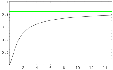
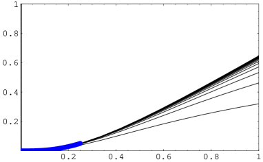
Figure 1: Left: Plot of $h_{23}(z)$ with asymptotic value $8/3\pi$. Right: Plot of the partial sums in $c_{23}(g)$ with weak coupling expansion up to radius of convergence $g={\textstyle\frac{1}{4}}$.

It is now possible to connect to strong coupling. The expansion of the function $h_{2,3}$ at large positive $z$ is

$$h_{2,3}(z)=\frac{8}{3\pi}-\frac{1}{z}+\frac{3\log(16z)}{4\pi z^{2}}-\frac{5}{8\pi z^{2}}+\frac{5\log(16z)}{512\pi z^{4}}+\frac{1}{2048\pi z^{4}}+\ldots\,.$$ (3.22)

Zeta function regularization of the sum yields

$$\sum_{k=1}^{\infty}h_{2,3}(g/k)\mathrel{} = \mathrel{}g\int_{0}^{\infty}h_{2,3}(1/z)\,dz+\frac{8\zeta(0)}{3\pi}-\frac{\zeta(-1)}{g}$$ (3.23)

$$\mathord{}+\frac{3}{4\pi}\,\frac{\zeta^{\prime}(-2)}{g^{2}}-\frac{5}{8\pi}\,\frac{\zeta(-2)}{g^{2}}+\frac{5}{512\pi}\,\frac{\zeta^{\prime}(-4)}{g^{4}}-\frac{1}{2048\pi}\,\frac{\zeta(-4)}{g^{4}}+\ldots$$

$$= \mathrel{}g-\frac{4}{3\pi}+\frac{1}{12g}-\frac{3\zeta(3)}{16\pi^{3}g^{2}}+\frac{15\zeta(5)}{2048\pi^{5}g^{4}}+\ldots$$

$$= \mathrel{}\sum^{\infty}_{n=0}c^{(n)}_{2,3}g^{1-n}.$$

Here the sum over $k^{n}$ is regularized to $\zeta(-n)$ while the sum over $k^{n}\log(k)$ yields $-\zeta^{\prime}(-n)$. We have verified the perfect agreement of the expansion with the strong-coupling coefficients $c^{(n)}_{2,3}$ to order $g^{-100}$ leaving little room for error. In App. C we present a proof of this statement to all orders. In the proof we observe some exponential corrections of the type $\mathcal{O}(e^{-g})$ to the series. These corrections are not unexpected because the series is asymptotic. A plot of the partial sums and asymptotic strong-coupling expansion of $c_{2,3}$ is given in Fig. 2.

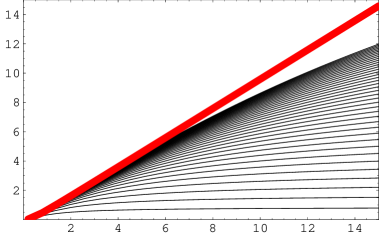
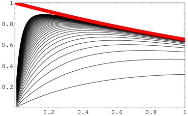
Figure 2: Left: Plot of partial sums in $c_{2,3}(g)$ with asymptotic strong coupling expansion. Right: We have plotted $xc_{2,3}(1/x)$ instead to improve the view of the strong-coupling behavior.

We have also confirmed the same agreement for other values of $(r,s)$: We can always replace the $\zeta(1+2n)$ in $c_{r,s}$ by a new sum and write $c_{r,s}$ in terms of a function $h_{r,s}(z)$ without odd-zeta terms

$$c_{r,s}(g)=\sum_{k=1}^{\infty}h_{r,s}(g/k).$$ (3.24)

The series in $g$ can now be written formally as the hypergeometric function

$$h_{r,s}(z)=\frac{2\cos[{\textstyle\frac{1}{2}}\pi(s-r-1)]\mathop{\smash{\Gamma}\vphantom{a}}\nolimits(r+s-2)}{\mathop{\smash{\Gamma}\vphantom{a}}\nolimits(r-1)\mathop{\smash{\Gamma}\vphantom{a}}\nolimits(s-1)}\,z^{r+s-2}\,\mathop{{}_{4}\smash{\operator@font F}_{3}\vphantom{a}}\nolimits(\vec{a};\vec{b};-16z^{2})$$ (3.25)

with arguments $\vec{a}=[{\textstyle\frac{1}{2}}(r+s-2),{\textstyle\frac{1}{2}}(r+s-1),{\textstyle\frac{1}{2}}(r+s-1),{\textstyle\frac{1}{2}}(r+s)]$ and $\vec{b}=[r,s,r+s-1]$. This hypergeometric function can be evaluated to the general form using elliptic integrals

$$h_{r,s}(z)=\frac{P_{r,s}(z^{2})}{z^{r+s-2}}+\frac{Q_{r,s}(z^{2})}{\pi z^{r+s-2}}\,\mathop{\smash{\operator@font K}\vphantom{a}}\nolimits(4iz)+\frac{R_{r,s}(z^{2})}{\pi z^{r+s-2}}\,\mathop{\smash{\operator@font E}\vphantom{a}}\nolimits(4iz).$$ (3.26)

Here $P,Q,R$ are some polynomials of degree $(r+s-3)/2$ with rational coefficients. The polynomials $P$ and $R$ have special factors for all value of $r,s$, namely $P(z^{2})\sim z^{2(r-2)}$ and $Q(z^{2})\sim(1+16z^{2})$. As in the above case of $(r,s)=(2,3)$, we use zeta function regularization to evaluate the sums (3.24) at strong coupling. We have further expanded some of the functions (3.25) at strong coupling and they fully agreed with the proposal in [29] upon zeta function regularization in all cases tested (all pairs of $r,s$ with $s\leq 10$ to 20 orders). In App. C we will finally show for general $(r,s)$ that $c_{r,s}(g)$ at large $g$ yields the first two orders $c^{(0)}_{r,s}$ and $c^{(1)}_{r,s}$ in (3.5) which are known from perturbative string theory [25, 41].

It is therefore fair to claim that the strong-coupling expansion (3.3) and the weak-coupling expansion (3.11) describe one and the same function $c_{r,s}(g)$ for all $(r,s)$. However, we should stress that the weak-coupling expansion is more versatile than the strong-coupling one: The functions $h_{r,s}$ have singularities at $g=\pm\frac{i}{4}$, and thus the coefficients $c_{r,s}(g)$ have singularities at $g=\pm\frac{i}{4}k$ for all positive integers $k$. Consequently, $c_{r,s}(g)$ has a finite radius of convergence around $g=0$, and the weak-coupling series defines the function unambiguously. In contradistinction the strong-coupling expansion is merely asymptotic and does not fully define the function.

4 Magic Kernels

Now we will return to our study of the integral equation for the fluctuation density in the presence of a perturbative dressing phase $\theta\neq 0$. As noted in section 2, there appears to exist a very special choice for the constants $\beta_{r,s}^{(\ell)}$ in (2.10) such that the odd-zeta contributions to the scaling function based on a trivial phase $\theta=0$ ($f_{\mathrm{m}}(g)$, see (2.8)) either cancel ($f_{0}(g)$, see (2.20)), or synchronize their relative sign w.r.t. the even-zeta contributions ($f(g)$, see (2.22)). The constants of the latter case appeared to differ from the ones of the former case by a factor of two. Let us now prove these statements, and derive the relevant set of constants $\beta_{r,s}^{(\ell)}$.

An observation of central importance for this section is that the simplified scaling function $f_{0}(g)$ may be obtained from an effective kernel much simpler than (2.13,2). One just needs to decompose the “main scattering” kernel (2.6) into two parts

$$\hat{K}_{\mathrm{m}}(t,t^{\prime})=\hat{K}_{0}(t,t^{\prime})+\hat{K}_{1}(t,t^{\prime}),$$ (4.1)

which are even and odd functions, respectively, under both $t\to-t$, $t^{\prime}\to-t^{\prime}$. Explicitly these functions read

$$\hat{K}_{0}(t,t^{\prime})\mathrel{} = \mathrel{}\frac{t\mathop{\smash{J_{1}}\vphantom{a_{1}}}\nolimits(t)\mathop{\smash{J_{0}}\vphantom{a_{0}}}\nolimits(t^{\prime})-t^{\prime}\mathop{\smash{J_{0}}\vphantom{a_{0}}}\nolimits(t)\mathop{\smash{J_{1}}\vphantom{a_{1}}}\nolimits(t^{\prime})}{t^{2}-t^{\prime 2}}\,,$$

$$\hat{K}_{1}(t,t^{\prime})\mathrel{} = \mathrel{}\frac{t^{\prime}\mathop{\smash{J_{1}}\vphantom{a_{1}}}\nolimits(t)\mathop{\smash{J_{0}}\vphantom{a_{0}}}\nolimits(t^{\prime})-t\mathop{\smash{J_{0}}\vphantom{a_{0}}}\nolimits(t)\mathop{\smash{J_{1}}\vphantom{a_{1}}}\nolimits(t^{\prime})}{t^{2}-t^{\prime 2}}\,.$$ (4.2)

It turns out that the component $\hat{K}_{1}$ is responsible for all odd-zeta contributions to $f_{\mathrm{m}}$. If we eliminate it and set $\hat{K}=\hat{K}_{0}$ in (2.2) we obtain just the same functions $\hat{\sigma}_{0}$ and $f_{0}(g)$, see (2.20). Note that again (2.4) remains true under this symmetrization, and (2.7) holds with $\hat{K}_{\mathrm{m}}\to\hat{K}_{0}$.

We can use this observation to obtain an almost closed expression for the dressing kernel. We start from the integral equation with a purely even kernel (4)

$$\hat{\sigma}_{0}(t)=\frac{t}{e^{t}-1}\Bigl{[}\hat{K}_{0}(2\,g\,t,0)-4\,g^{2}\int_{0}^{\infty}dt^{\prime}\;\hat{K}_{0}(2\,g\,t,2\,g\,t^{\prime})\,\hat{\sigma}_{0}(t^{\prime})\Bigr{]},$$ (4.3)

which leads to $f_{0}(g)$. Replacing $\hat{K}_{0}$ by $\hat{K}_{\mathrm{m}}-\hat{K}_{1}$, using $\hat{K}_{1}(t,0)=0$, and substituting $\hat{\sigma}_{0}$ once into the ensuing second convolution only, we derive the relation

$$\hat{\sigma}_{0}(t)\mathrel{} = \mathrel{}\frac{t}{e^{t}-1}\Bigl{[}\hat{K}_{\mathrm{m}}(2\,g\,t,0)+\hat{K}_{\mathrm{c}}(2\,g\,t,0)$$ (4.4)

$$\mathord{}\qquad\qquad-4\,g^{2}\int_{0}^{\infty}dt^{\prime}\;\left(\hat{K}_{\mathrm{m}}(2\,g\,t,2\,g\,t^{\prime})+\hat{K}_{\mathrm{c}}(2\,g\,t,2\,g\,t^{\prime})\right)\hat{\sigma}_{0}(t^{\prime})\Bigr{]}.$$

with the function $\hat{K}_{\mathrm{c}}$

$$\hat{K}_{\mathrm{c}}(t,t^{\prime})=4\,g^{2}\,\int_{0}^{\infty}dt^{\prime\prime}\,\hat{K}_{1}(t,2\,g\,t^{\prime\prime})\,\frac{t^{\prime\prime}}{e^{t^{\prime\prime}}-1}\,\hat{K}_{0}(2\,g\,t^{\prime\prime},t^{\prime}).$$ (4.5)

Now (4.4) is just the original integral equation (2.2), but with the kernel $\hat{K}=\hat{K}_{\mathrm{m}}+\hat{K}_{\mathrm{c}}$. Therefore we can interpret $\hat{K}_{\mathrm{c}}$ as a dressing kernel to generate the simplified dressing function $f_{0}(g)$. In fact, it agrees precisely with the expansion of the general dressing kernel (2.13,2) using the first few coefficients found in (2.19)! The expression for the dressing kernel $\hat{K}_{\mathrm{c}}$ allows us to derive a closed expression for the constants $\beta_{r,s}^{(\ell)}$ leading to cancellation of odd-zeta contributions. The details of this derivation are presented in App. A, the final result is

$$\beta_{r,r+1+2\nu}^{(r+\nu+\mu)}\to(-1)^{r+\mu+1}\,\frac{(r-1)(r+2\nu)}{2\mu+1}\,\left(\genfrac{}{}{0.0pt}{}{2\mu+1}{\mu-r-\nu+1}\right)\left(\genfrac{}{}{0.0pt}{}{2\mu+1}{\mu-\nu}\right)\zeta(2\mu+1)\,.$$ (4.6)

Surprisingly, these coefficients agree, up to a global factor of ${\textstyle\frac{1}{2}}$, with the “analytic continuation” of the conjectured strong-coupling dressing phase constants (3.13,3.16)! The results of the previous section then suggest that the correct crossing-invariant choice of constants is just twice (4.6). Of course, these constants agree with those in (2.21). The corresponding kernel for the integral equation (2.2) of the universal scaling function $f(g)$ is, cf. (2.6,4.5)

$$\hat{K}(t,t^{\prime})=\hat{K}_{\mathrm{m}}(t,t^{\prime})+2\,\hat{K}_{\mathrm{c}}(t,t^{\prime})\,.$$ (4.7)

What does this imply for the universal scaling function? We “experimentally” observed in section 2, to rather high order, that the doubled constants (4.8) lead to sign-reversals in those odd-zeta terms which do not have the same relative sign as the even-zeta terms in the original proposal (2.8). Up to this minor modification, the associated scaling function agrees with the one based on a trivial phase. We will present a proof of this statement in App. B.

It is interesting to investigate the analytic structure of the three candidate scaling functions. In each case one would like to find the locations of all singularities in the complex $g$-plane, and determine wether they correspond to poles, branch points, or are of essential type. The convergence properties of the weak coupling expansion series are, in particular, clearly related to the singularity with smallest $|g|$.

The integral form of the dressing kernel $K_{\mathrm{c}}$ allows to derive conveniently the first few orders in the expansion of the scaling function. The analytic expression is given (2.22). Beyond $20$ orders, however, the analytic calculation slowed down substantially due to an exploding number of partitions for the odd-zeta contributions. This complexity can be reduced by reverting to a numerical computation. We were able to produce all three scaling functions $f_{\mathrm{m}}(g)$, $f_{0}(g)$ and $f(g)$ up to $50$ loops, $\mathcal{O}(g^{100})$, at $1000$-digit accuracy (needed for intermediate steps). A plot of these three functions is shown in Fig. 3.

Figure 3: Top to bottom curve: Plot of the scaling functions $f_{\mathrm{m}}(g)$, $f_{0}(g)$ and $f(g)$ with $g={\textstyle\frac{1}{4}}\sqrt{x}$.

We have then used the quotient criterion to investigate the convergence properties of the series. Our results indicate that the radius of convergence in $g$ is ${\textstyle\frac{1}{4}}$ in all three cases. The related singularity is situated at $g=\pm\frac{i}{4}$ or, put differently, at $\lambda=-\pi^{2}$. The accuracy of this result was very high and the position matches with the singularity of the function in (3.21). The exponents of the singularity $f\simeq(\lambda+\pi^{2})^{\alpha}$ appear to be $\alpha=+1,+\frac{2}{3},+\frac{1}{2}$ for the three functions $f_{\mathrm{m}}(g)$, $f_{0}(g)$, $f(g)$, respectively. We were not able to produce a very accurate result in this case, we expect it to be accurate within a few percent.

In conclusion, the final proposal for the, hopefully correct, expansion coefficients of the dressing phase (2.10,2.11) reads

$$\beta_{r,r+1+2\nu}^{(r+\nu+\mu)}=2(-1)^{r+\mu+1}\,\frac{(r-1)(r+2\nu)}{2\mu+1}\,\left(\genfrac{}{}{0.0pt}{}{2\mu+1}{\mu-r-\nu+1}\right)\left(\genfrac{}{}{0.0pt}{}{2\mu+1}{\mu-\nu}\right)\zeta(2\mu+1)\,.$$ (4.8)

The resulting universal scaling function $f(g)$ in a weak-coupling expansion was presented in (2.22) to the first few orders. Its convergence properties seem to indicate a singularity at $\lambda=-\pi^{2}$ with exponent $+\frac{1}{2}$.

The strong-coupling expansion of the scaling function $f(g)$ remains to be evaluated within the Bethe ansatz framework. A comparison to available data [53, 54] from string theory would constitute an important test of our proposed dressing phase. The leading order at strong coupling based on the AFS phase [25] (which is consistent with our proposal) indeed agrees [55] with an explicit string theory calculation [53]. Conversely, in the case of the un-dressed function $f_{\mathrm{m}}(g)$, the integral equation is troublesome and leads to a fluctuating solution [36]. Hopefully the situation is improved by the correct dressing phase in order to find agreement with string theory.

5 Conclusions and Outlook

In this paper we have derived an expression (2.10,2.11,4.8) for the complete weak-coupling expansion of the dressing phase $\theta$ in the Bethe ansatz [7] of planar $\mathcal{N}=4$ gauge theory. It is based on a crossing-symmetric proposal in Sec. 5.2 of [29] for the strong-coupling expansion of the dressing phase in conjunction with some curious structures of cancellations and replacements when a dressing phase modifies the scaling function $f_{\mathrm{m}}(g)$ based on a trivial phase, as originally derived in [16]. Whether or not our proposal describes the AdS/CFT system accurately, we have shown that there exists a natural expression for the dressing phase which appears to interpolate between currently known spectral data at weak and strong coupling. We are hopeful, but have not shown, that any alteration of our proposal is likely to violate the transcendentality principle in gauge theory and/or crossing symmetry in string theory as well as leads to potential contradictions with the available data. In that sense our proposal lends support to an exact interpretation of the AdS/CFT correspondence [20, 21, 22], at least in the case of $\mathcal{N}=4$ gauge theory in the ’t Hooft limit and free IIB superstrings on $AdS_{5}\times S^{5}$.

The dressing phase $\theta$ is given as a multiple expansion in excitation charges and the coupling constant. The radius of convergence w.r.t. the ’t Hooft coupling $\lambda$ around $\lambda=0$ is $|\lambda|<\pi^{2}$. The singularities are situated at $\lambda=-n^{2}\pi^{2}$ for all non-zero integers $n$. Consequently, perturbative gauge theory appears to unambiguously define the phase and its analytic continuation. Note however that we have not succeeded in summing over the modes $r,s$ of $\beta_{r,s}(g)$ or even study the analytic structure of the phase $\theta$ in general. Conversely, the strong-coupling expansion of the phase can merely be asymptotic because $\lambda=\infty$ is an accumulation point of singularities. The asymptotic string expansion proposed in Sec. 5.2 of [29] seems to be in perfect agreement with our proposal, but it is not sufficient to uniquely define a complex function.

Two methods of testing our coefficients come to mind: The first is a direct computation of the scaling function $f(g)$ at four loops. Until recently, it was known up to three loops [8, 9], see also [11], but with methods based on the unitarity of scattering amplitudes it is within computational reach [13, 14, 15]. Our prediction $\beta^{(3)}_{2,3}=4\beta=4\zeta(3)$ leads to a four-loop contribution to the universal scaling function

$$f(g)\mathrel{} = \mathrel{}\ldots-16\,\left(\frac{73}{630}\,\pi^{6}+4\,\zeta(3)^{2}\right)\,g^{8}\,+\ldots$$ (5.1)

$$\approx \mathrel{}\ldots-3.01502\times 10^{-6}\lambda^{4}+\ldots\,.$$

The final outcome of the four-loop calculation by Bern, Czakon, Dixon, Kosower and Smirnov [15], which was performed in parallel and completely independently from our analysis, is

$$f(g)\mathrel{} = \mathrel{}\ldots-64\times\left(29.335\pm 0.052\right)\,g^{8}\,+\ldots$$ (5.2)

$$= \mathrel{}\ldots-\bigl{(}3.0192\pm 0.0054\bigr{)}\times 10^{-6}\lambda^{4}+\ldots\,.$$

The perfect agreement between the two numbers provides further confidence that our proposed dressing phase correctly describes the asymptotic spectrum of anomalous dimensions in planar $\mathcal{N}=4$ gauge theory. At the least it ascertains that the dressing phase is non-trivial starting from $\mathcal{O}(g^{6})$, and that the constant for the first correction in [16] takes the value $\beta={\textstyle\frac{1}{4}}\beta^{(3)}_{2,3}=\zeta(3)$. Note, however, that we have to assume the exact universality of the scaling function, i.e. that it is exactly the same for twist-two (as assumed in [15]) and for higher-twist (as required for the asymptotic Bethe ansatz).

A computation of the function $f(g)$ to even higher loop orders would provide more stringent tests of our proposal. Given the remarkable success of unitarity-based methods in [8, 9, 15] we do not dare calling this impracticable. However, some yet-to-be-discovered iterative structure is likely to exist if our comparably simple integral equation holds true. With many perturbative orders available an extrapolation to strong coupling may be attempted and compared to string theory results [53, 54] via the AdS/CFT correspondence. Such an analysis was indeed performed in [15] using the KLV [56] and Padé approximations. It is based on their independent guess of the function $f(g)$ in (2.22) and how to obtain it from the earlier proposal (2.8) by synchronizing all signs. Strangely, their approximations, based on using the first seven or eight terms for example, appear to indicate that (2.22) is about $5\%$ away from the expected strong-coupling value of [53]. Non-coincidence of the values would be rather puzzling with regard to the discussion at the end of Sec. 4 and Sec. 3. Would it imply that $f(g)$ at strong coupling does not describe the string states in [53, 54]? Are there some non-perturbative corrections? To that end, it would be worth investigating whether an adapted scheme which takes into account all singularities at $\lambda=-n^{2}\pi^{2}$ and their accumulation at $\lambda=\infty$ can produce an extrapolation of $f(g)$ closer to the expected string theory values [53, 54].

Another way of testing the proposal involves local operators of small classical dimension. A gauge Bethe ansatz modified by a dressing phase changes the anomalous dimensions $\mathnormal{\Delta}$ of all operators in all sectors. E.g. in the $\mathfrak{su}(2)$ sector we would find for the length $L=5$ operator $\mathop{\mathrm{Tr}}X^{2}\,Z^{3}+\ldots$ (this case is actually equivalent to the $\mathfrak{sl}(2)$ twist=length three operator $\mathop{\mathrm{Tr}}D^{2}\,Z^{3}+\ldots$) to four loops

$$\mathnormal{\Delta}=5+8\,g^{2}-24\,g^{4}+136\,g^{6}-16\,\bigl{(}{\textstyle\frac{115}{2}}+2\,\beta_{2,3}^{(3)}\bigr{)}\,g^{8}\,+\ldots\,.$$ (5.3)

For the specific case of constants (4.8) we then have

$$\mathnormal{\Delta}=5+8\,g^{2}-24\,g^{4}+136\,g^{6}-16\,\bigl{(}{\textstyle\frac{115}{2}}+8\,\zeta(3)\bigr{)}\,g^{8}\,+\ldots\,.$$ (5.4)

Intriguingly, this predicts the appearance of a non-rational term in the four-loop anomalous dimension of a finite length operator! Such contributions are impossible if the dressing phase is trivial, i.e. if $\theta=0$. They are certainly not excluded, and a priori even likely, from the point of view of perturbative field theory. This would then also rule out the all-loop “BDS” ansatz originally proposed in [33], and as a consequence also its finite-length description through the Lieb-Wu equations of the Hubbard model, cf. (68) in [57]. It also eliminates the Hubbard Hamiltonian as an exact candidate for the $\mathfrak{su}(2)$ dilatation operator [57]. However, a gauge theory dressing phase (2.10) whose constants preserve transcendentality for twist operators, such as in the specific suggestion (4.8), would have the following intriguing property affecting operators of finite length and spin: Up to (at least) wrapping order, the BDS ansatz would give the correct “rational part” of all anomalous dimension matrices, and the Hubbard Hamiltonian would emulate the “rational part” of the $\mathfrak{su}(2)$ dilatation operator to (at least) wrapping order.

An interesting question concerns the computation of anomalous dimensions beyond wrapping order. The simplest case is the four-loop anomalous dimension of the Konishi field, i.e. the $\mathfrak{su}(2)$ length $L=4$ operator $\mathop{\mathrm{Tr}}X^{2}\,Z^{2}+\ldots$, or, equivalently, in $\mathfrak{sl}(2)$ the lowest spin $S=2$, length $L=2$ operator $\mathop{\mathrm{Tr}}D^{2}\,Z^{2}+\ldots$. If we, a priori “illegally”, apply the asymptotic Bethe ansatz (2.9,2.10) we find the four-loop result

$$\mathnormal{\Delta}=4+12\,g^{2}-48\,g^{4}+336\,g^{6}-16\,\bigl{(}{\textstyle\frac{705}{4}}+{\textstyle\frac{9}{2}}\,\beta_{2,3}^{(3)}\bigr{)}\,g^{8}\,+\ldots\,.$$ (5.5)

Recall that $\beta_{2,3}^{(3)}=0$ is the “BDS” case with dressing phase $\theta=0$. With our conjecture (4.8) we then have instead

$$\mathnormal{\Delta}=4+12\,g^{2}-48\,g^{4}+336\,g^{6}-16\,\bigl{(}{\textstyle\frac{705}{4}}+18\,\zeta(3)\bigr{)}\,g^{8}\,+\ldots\,.$$ (5.6)

However, as opposed to (5.4), this result is much less certain. It would only be true if our asymptotic Bethe equations turn out to be exact. Conversely, recall that the Hubbard model [57] yields for this state

$$\mathnormal{\Delta}=4+12\,g^{2}-48\,g^{4}+336\,g^{6}-16\times 318\,g^{8}+\ldots\,.$$ (5.7)

Could it be that the Hubbard model still properly yields the “rational part” of fields even beyond wrapping order? This might then result in

$$\mathnormal{\Delta}=4+12\,g^{2}-48\,g^{4}+336\,g^{6}-16\,\bigl{(}318+18\,\zeta(3)\bigr{)}\,g^{8}\,+\ldots\,,$$ (5.8)

but, in the absence of a yet-to-be constructed rigorous Bethe ansatz for the finite system, this is of course a quite unfounded speculation.

Of course, there are more general questions: It would be very valuable to find a closed form for the proposed dressing phase $\theta$ and to prove its correctness. Likewise, the exact integrability of the planar AdS/CFT model still lacks a rigorous proof. Are the Bethe equations at finite coupling and finite length exact or is there a more fundamental description of the planar spectrum of which the Bethe equations are merely some limits? For instance, the exactness may be flawed by certain terms which are exponentially suppressed at long states [58, 59]. The “covariant” approaches started in [60, 57, 61, 62] may provide an answer to this question as well as recover the dressing phase from a more fundamental (and simpler) description. Other promising approaches are the thermodynamical Bethe ansatz (see [63]) and Baxter equations (see [64, 65]).

It is curious to see that in our proposal the deviations from a trivial phase start to contribute to anomalous dimensions at four loops, which is a rather high perturbative order. If true, this might indicate that intuition gained from some perturbative computations, even if they extend to two or three loops, may be deceiving. For instance, a non-zero value for $\beta^{(3)}_{2,3}=4\beta$ leads to a four-loop breakdown of weak-coupling BMN-scaling [2] in $\mathcal{N}=4$ gauge theory. This possibility was discussed by several authors in the past in order to reconcile discrepancies between gauge and string theory structures at, respectively weak and strong coupling. See in particular [66, 19, 33, 67, 40, 68, 69]. Our proposal suggests that this is indeed the case. The assumption of [2] that the BMN limit leads to a dilute gas with weakly interacting particles is not compatible with our phase. It should be noted that the perturbative dispersion relation obtained in [70, 71] is indeed compatible with our proposal. However, it cannot be translated directly into anomalous dimensions of local operators as suggested in [2, 70, 71].

The same applies for the spinning strings proposal [72]: The weak-coupling expansion in the effective coupling constant $\lambda^{\prime}\sim\lambda/J^{2}$ leads to terms of the type $(\lambda^{\prime})^{4}J^{2}$ which diverge in the limit of large spin $J$. The investigation of spinning string solutions from the gauge theory side started in [73] will therefore fatally break down at the four-loop level. Nevertheless, the proposals [2, 72] have been of tremendous importance to initiate the study of stringy and integrable structures in $\mathcal{N}=4$ gauge theory.

Finally, it is worth pointing out that $\beta_{2,3}(g)=\mathcal{O}(g^{6})$ is reminiscent of the findings [74] within the plane wave (BMN) matrix model [2]. Also there, a non-trivial dressing phase was observed starting at the same order. The main difference is that the coefficient $\beta_{2,3}^{(3)}$ for the BMN matrix model is rational while ours is a rational multiple of $\zeta(3)$. This may potentially be related to the fact that the matrix model has only finitely many degrees of freedom while $\mathcal{N}=4$ SYM is non-compact.

Acknowledgements

We are grateful to Z. Bern, M. Czakon, L. Dixon, D. Kosower and V. Smirnov for supplying us with a draft of their manuscript [15], and for discussions as well as comments on our draft. We would also like to sincerely thank them for undertaking such a tremendously important and impressive effort. We furthermore thank S. Frolov, E. López, J. Plefka and D. Serban for comments on the manuscript.

Appendix A Expansion of the Magic Kernel

In this appendix we present a weak-coupling expansion of the magic kernel $\hat{K}_{\mathrm{c}}$ in (4.5) leading to an expression for the coefficients $\beta^{(\ell)}_{r,s}$ of the dressing phase.

A useful integral representation for the even and odd parts was found in [16]:

$$\hat{K}_{0}(t,t^{\prime})\mathrel{} = \mathrel{}\int_{0}^{1}d\lambda\,\lambda\,\mathop{\smash{J_{0}}\vphantom{a_{0}}}\nolimits(\lambda\,t)\mathop{\smash{J_{0}}\vphantom{a_{0}}}\nolimits(\lambda\,t^{\prime})\,,$$

$$\hat{K}_{1}(t,t^{\prime})\mathrel{} = \mathrel{}\int_{0}^{1}d\lambda\,\lambda\,\mathop{\smash{J_{1}}\vphantom{a_{1}}}\nolimits(\lambda\,t)\mathop{\smash{J_{1}}\vphantom{a_{1}}}\nolimits(\lambda\,t^{\prime})\,.$$ (A.1)

With their help, we may calculate $\hat{K}_{\mathrm{c}}$ to be

$$\hat{K}_{\mathrm{c}}(t,t^{\prime})\mathrel{} = \mathrel{}4g^{2}\int_{0}^{\infty}dt^{\prime\prime}\;\int_{0}^{1}d\lambda_{1}\,\lambda_{1}\mathop{\smash{J_{1}}\vphantom{a_{1}}}\nolimits(\lambda_{1}\,t)\mathop{\smash{J_{1}}\vphantom{a_{1}}}\nolimits(\lambda_{1}\,2\,g\,t^{\prime\prime})\;\frac{t^{\prime\prime}}{e^{t^{\prime\prime}}\,-\,1}\,\times$$ (A.2)

$$\mathord{}\phantom{2g^{2}\int_{0}^{\infty}dt^{\prime\prime}\;}\int_{0}^{1}d\lambda_{2}\,\lambda_{2}\,\mathop{\smash{J_{0}}\vphantom{a_{0}}}\nolimits(\lambda_{2}\,2\,g\,t^{\prime\prime})\mathop{\smash{J_{0}}\vphantom{a_{0}}}\nolimits(\lambda_{2}\,t^{\prime})$$

$$= \mathrel{}-4\sum_{\mu=1}^{\infty}(-1)^{\mu}g^{2\mu+1}\zeta(2\mu+1)\;(2\mu)!\,\times$$

$$\mathord{}\qquad\sum_{n=0}^{\mu-1}\frac{1}{n!\,(n+1)!\,(\mu-1-n)!\,(\mu-1-n)!}\,\times$$

$$\mathord{}\qquad\int_{0}^{1}d\lambda_{1}\,\lambda_{1}^{2(n+1)}\mathop{\smash{J_{1}}\vphantom{a_{1}}}\nolimits(\lambda_{1}\,t)\,\int_{0}^{1}d\lambda_{2}\,\lambda_{2}^{2(\mu-n)-1}\mathop{\smash{J_{0}}\vphantom{a_{0}}}\nolimits(\lambda_{2}\,t^{\prime})$$

where we have first expanded the Bessel functions with argument $\lambda_{1,2}\,2\,g\,t^{\prime\prime}$ in $g$ and then executed the $t^{\prime\prime}$ integration. The two remaining parameter integrals in the last line may be found from a standard formula. In the first integral the power of $\lambda_{1}$ in front of $\mathop{\smash{J_{1}}\vphantom{a_{1}}}\nolimits(\lambda_{1}t)$ is always even, and in the second one the power of $\lambda_{2}$ in front of $\mathop{\smash{J_{0}}\vphantom{a_{0}}}\nolimits(\lambda_{2}t^{\prime})$ is always odd. Both integrals therefore yield finite sums of Bessel functions:

$$\mathrel{}\int_{0}^{1}d\lambda_{1}\,\lambda_{1}^{2m}\mathop{\smash{J_{1}}\vphantom{a_{1}}}\nolimits(\lambda_{1}\,t)$$ (A.3)

$$= \mathrel{}-\frac{(m-1)!\,m!}{(2m)!}\sum_{k=1}^{m}(-1)^{k}\begin{pmatrix}2m\\ m-k\end{pmatrix}\frac{2k}{t}\mathop{\smash{J_{2k}}\vphantom{a_{2k}}}\nolimits(t)$$

$$\mathrel{}\int_{0}^{1}d\lambda_{2}\,\lambda_{2}^{2m-1}\mathop{\smash{J_{0}}\vphantom{a_{0}}}\nolimits(\lambda_{2}\,t^{\prime})$$

$$= \mathrel{}-\frac{(m-1)!\,(m-1)!}{(2m-1)!}\sum_{l=1}^{m}(-1)^{l}\begin{pmatrix}2m-1\\ m-l\end{pmatrix}\frac{2l-1}{t^{\prime}}\,\mathop{\smash{J_{2l-1}}\vphantom{a_{2l-1}}}\nolimits(t^{\prime})\,.$$

On substituting these into (A.2) we can cancel the factors which depend on $n$ but not on $k,l$. We re-order the $n,k,l$ sums to find:

$$\hat{K}_{\mathrm{c}}(t,t^{\prime})\mathrel{} = \mathrel{}-\frac{4}{t\,t^{\prime}}\sum_{\mu=1}^{\infty}(-1)^{\mu}g^{2\mu+1}\zeta(2\mu+1)\;(2\mu)!\,\times$$ (A.4)

$$\mathord{}\qquad\sum_{k,l\geq 1}^{k+l\leq\mu+1}(-1)^{k+l}(2k)\mathop{\smash{J_{2k}}\vphantom{a_{2k}}}\nolimits(t)\;(2l-1)\mathop{\smash{J_{2l-1}}\vphantom{a_{2l-1}}}\nolimits(t^{\prime})\,\times$$

$$\mathord{}\qquad\sum_{n=k-1}^{\mu-l}\frac{1}{(n+1-k)!\,(n+1+k)!\,(\mu-l-n)!\,(\mu+l-1-n)!}\,.$$

The sum over $n$ can be done in closed form:

$$\mathrel{}\sum_{n=k-1}^{\mu-l}\frac{1}{(n+1-k)!\,(n+1+k)!\,(\mu-l-n)!\,(\mu+l-1-n)!}$$ (A.5)

$$= \mathrel{}\frac{1}{(2\mu+1)!}\begin{pmatrix}2\mu+1\\ \mu+1-k-l\end{pmatrix}\begin{pmatrix}2\mu+1\\ \mu+1+k-l\end{pmatrix}\,.$$

Collecting results, we get

$$\hat{K}_{\mathrm{c}}(t,t^{\prime})\mathrel{} = \mathrel{}-\frac{4}{t\,t^{\prime}}\sum_{\mu=1}^{\infty}g^{2\mu+1}\,\sum_{k,l\geq 1}^{k+l\leq\mu+1}\mathop{\smash{J_{2k}}\vphantom{a_{2k}}}\nolimits(t)\mathop{\smash{J_{2l-1}}\vphantom{a_{2l-1}}}\nolimits(t^{\prime})\,(-1)^{\mu+k+l}\,\times$$ (A.6)

$$\mathord{}\qquad\frac{(2k)\,(2l-1)}{2\mu+1}\begin{pmatrix}2\mu+1\\ \mu+1-k-l\end{pmatrix}\begin{pmatrix}2\mu+1\\ \mu+1+k-l\end{pmatrix}\zeta(2\mu+1)\,.$$

This is precisely of the form of a kernel stemming from a non-trivial dressing phase $\theta$, as we can see by comparing to (2)! We can even read off the constants $\beta_{r,s}^{(\ell)}$:

$$\beta_{r,r+1+2\nu}^{(r+\nu+\mu)}\to(-1)^{r+\mu+1}\,\frac{(r-1)(r+2\nu)}{2\mu+1}\,\left(\genfrac{}{}{0.0pt}{}{2\mu+1}{\mu-r-\nu+1}\right)\left(\genfrac{}{}{0.0pt}{}{2\mu+1}{\mu-\nu}\right)\zeta(2\mu+1)\,.$$ (A.7)

Finally, instead of using the integral representation (A), we may also cast the two kernels $\hat{K}_{0}$, $\hat{K}_{1}$ in the form of infinite sums:

$$\hat{K}_{0}(t,t^{\prime})\mathrel{} = \mathrel{}\frac{2}{t\,t^{\prime}}\sum_{n=0}^{\infty}(2n+1)\mathop{\smash{J_{2n+1}}\vphantom{a_{2n+1}}}\nolimits(t)\mathop{\smash{J_{2n+1}}\vphantom{a_{2n+1}}}\nolimits(t^{\prime})\,,$$

$$\hat{K}_{1}(t,t^{\prime})\mathrel{} = \mathrel{}\frac{2}{t\,t^{\prime}}\sum_{n=1}^{\infty}(2n)\mathop{\smash{J_{2n}}\vphantom{a_{2n}}}\nolimits(t)\mathop{\smash{J_{2n}}\vphantom{a_{2n}}}\nolimits(t^{\prime})\,.$$

It follows that

$$\hat{K}_{\mathrm{c}}(t,t^{\prime})=\frac{2}{t\,t^{\prime}}\sum_{k=1}^{\infty}\sum_{l=0}^{\infty}(-1)^{k+l}c_{2k+1,2l+2}(g)\mathop{\smash{J_{2k}}\vphantom{a_{2k}}}\nolimits(t)\mathop{\smash{J_{2l+1}}\vphantom{a_{2l+1}}}\nolimits(t^{\prime})$$ (A.8)

with the coefficient functions

$$c_{r,s}(g)=2\cos[{\textstyle\frac{1}{2}}\pi(s-r-1)]\,(r-1)(s-1)\int_{0}^{\infty}dt\,\frac{\mathop{\smash{J_{r-1}}\vphantom{a_{r-1}}}\nolimits(2\,g\,t)\mathop{\smash{J_{s-1}}\vphantom{a_{s-1}}}\nolimits(2\,g\,t)}{t(e^{t}-1)}\,.$$ (A.9)

We can use this form to present an alternative proof. We firstly expand $1/(e^{t}-1)$ into a geometric series and secondly rescale the integration variable $t$ by $g$ such that the integral will manifestly depend on the ratio $g/n$ only

$$c_{r,s}(g)\mathrel{} = \mathrel{}\sum_{n=1}^{\infty}h_{r,s}(g/n),$$ (A.10)

$$h_{r,s}(g/n)\mathrel{} = \mathrel{}2\cos[{\textstyle\frac{1}{2}}\pi(s-r-1)]\,(r-1)(s-1)\int_{0}^{\infty}\frac{dt}{t}\,\exp(-tn/g)\mathop{\smash{J_{r-1}}\vphantom{a_{r-1}}}\nolimits(2\,t)\mathop{\smash{J_{s-1}}\vphantom{a_{s-1}}}\nolimits(2\,t)\,.$$

The integral can now be performed and yields precisely the hypergeometric function derived earlier in (3.25).

The discussion of the strong-coupling behavior of the dressing phase is tantamount to an analysis of the strong-coupling limit of the integrals $c_{r,s}(g)$. In App. C we present, by way of example, the full expansion in the case $(r,s)=(2,3)$. We also show that (A.10) reproduces the AFS phase [25] as well as the Hernández-López correction [41].

Appendix B Flipping Odd-Zetas Contributions

Here we show that the replacement of the kernel $\hat{K}_{\mathrm{m}}\to\hat{K}_{\mathrm{m}}+2\hat{K}_{\mathrm{c}}$ leads to the simple replacement $\zeta(2n+1)\to i\zeta(2n+1)$ in the scaling function $f_{\mathrm{m}}(g)\to f(g)$.

Let

$$z(t)=\frac{t}{e^{t}-1}\,.$$ (B.1)

For any kernel $\hat{K}(2gt,2gt^{\prime})$ and any function $f(t)$ we define the product

$$(\hat{K}\mathop{\ast}f)(t)=\int_{0}^{\infty}dt^{\prime}\,\hat{K}(2\,g\,t,2\,g\,t^{\prime})\,z(t^{\prime})\,f(t^{\prime})\,.$$ (B.2)

The integral equation may be written as

$$\hat{\sigma}(t)=z(t)\left((\hat{K}_{0}+\hat{K}_{\mathrm{c}})(2\,g\,t,0)-4g^{2}\,\left((\hat{K}_{0}+\hat{K}_{1}+\hat{K}_{\mathrm{c}})\mathop{\ast}\frac{\hat{\sigma}}{z}\right)(t)\right)\,.$$ (B.3)

In the following we need not consider the internal $g$-dependence of the kernels. Within the radius of convergence of the iteration the solution of any Fredholm equation of the second type is the resolvent

$$\hat{\sigma}(t)=z(t)\sum_{n=0}^{\infty}\,(-4g^{2})^{n}\,\biggl{(}[(\hat{K}_{0}+\hat{K}_{1}+\hat{K}_{\mathrm{c}})\mathop{\ast}]^{n}\,P\biggr{)}(t)\,.$$ (B.4)

Here $P(t)=(\hat{K}_{0}+\hat{K}_{\mathrm{c}})(2gt,0)$ and $\hat{K}_{\mathrm{c}}(2gt,2gt^{\prime})=8g^{2}(\hat{K}_{1}\mathop{\ast}\hat{K}_{0})(2gt,\,2gt^{\prime})$. The Fredholm resolvent must have the form

$$\hat{\sigma}(t)=z(t)\sum_{\underline{n}}\,(-4g^{2})^{n}\,\eta_{\underline{n}}\,(W_{\underline{n}}\,\hat{K}_{0})(t)$$ (B.5)

because the dressing kernel $\hat{K}_{\mathrm{c}}$ consists itself of $\hat{K}_{0},\hat{K}_{1}$ which are convoluted by the star operation (and it also carries the appropriate extra power of the coupling constant). By $\underline{n}$ we denote a string built of $0,1$ with total length $n$, and $W_{\underline{n}}$ is the corresponding string of $\hat{K}_{0},\hat{K}_{1}$ acting on the potential $\hat{K}_{0}$ by the $\ast$ product defined above in (B.2). The $\eta_{\underline{n}}$ are numerical coefficients. The integral equation (B.3) determines these numbers uniquely: We substitute (B.5) into the equation and pick the $\mathcal{O}(g^{2(n+2)})$ terms. All words are assumed independent; in particular the four double iterations of an arbitrary word $W_{\underline{n}}$:

$$W_{0,0,\underline{n}}\,,\qquad W_{0,1,\underline{n}}\,,\qquad W_{1,0,\underline{n}}\,,\qquad W_{1,1,\underline{n}}\,.$$ (B.6)

This yields the four equations

$$\eta_{0,0,\underline{n}}\mathrel{} = \mathrel{}-\,\eta_{0,\underline{n}}\,,$$

$$\eta_{0,1,\underline{n}}\mathrel{} = \mathrel{}-\eta_{1,\underline{n}}\,,$$

$$\eta_{1,0,\underline{n}}\mathrel{} = \mathrel{}-\eta_{0,\underline{n}}-2\eta_{\underline{n}}\,,$$

$$\eta_{1,1,\underline{n}}\mathrel{} = \mathrel{}-\eta_{1,\underline{n}}\,.$$

The first two equations may be summarized as

$$\eta_{0,\underline{m}}=-\eta_{\underline{m}}$$ (B.7)

from which it follows that the third equation is:

$$\eta_{1,0,\underline{n}}=+\eta_{0,\underline{n}}.$$ (B.8)

Recursively, these equations imply that all the $\eta$ coefficients are merely signs. Second, (B.8) implies that the operation of appending $\hat{K}_{1}$ after $\hat{K}_{0}$ is the only one that induces a sign flip as opposed to the iteration of the main scattering kernel $\hat{K}_{\mathrm{m}}=\hat{K}_{0}+\hat{K}_{1}$ alone (in that case the second term in the r.h.s. of (B) would be absent so that $\eta_{1,\underline{m}}=-\eta_{\underline{m}}$, too).

Next, let

$$\mathcal{E}=\{t^{2l}\,:\;l\in\mathbb{N}_{0}\},\qquad\mathcal{O}=\{t^{2l+1}\,:\;l\in\mathbb{N}_{0}\},$$ (B.9)

denote the even and odd powers of $t$, respectively. In order to obtain the scaling functions at weak coupling we will eventually expand the kernels $\hat{K}_{0,1}(2gt,2gt^{\prime})$ in the coupling constant; $\hat{K}_{0}$ ($\hat{K}_{1}$) is even (odd) in both arguments, respectively. Let us consider any one term in the expansion of a kernel convoluted on a power of $t$ by the star product. We observe the graded structure

$$\begin{array}[]{lllllll}\hat{K}_{0}\,:&\mathcal{E}\mathrel{}&\rightarrow&\mathrel{}\mathcal{E}&:\qquad t^{2l}\mathrel{}&\mapsto&\mathrel{}\zeta(2m)\,t^{2l^{\prime}},\\ &\mathcal{O}\mathrel{}&\rightarrow&\mathrel{}\mathcal{E}&:\qquad t^{2l+1}\mathrel{}&\mapsto&\mathrel{}\zeta(2m+1)\,t^{2l^{\prime}},\\ \hat{K}_{1}\,:&\mathcal{E}\mathrel{}&\rightarrow&\mathrel{}\mathcal{O}&:\qquad t^{2l}\mathrel{}&\mapsto&\mathrel{}\zeta(2m+1)\,t^{2l^{\prime}+1},\\ &\mathcal{O}\mathrel{}&\rightarrow&\mathrel{}\mathcal{O}&:\qquad t^{2l+1}\mathrel{}&\mapsto&\mathrel{}\zeta(2m)\,t^{2l^{\prime}+1}.\end{array}$$ (B.10)

The first integral in a chain of convolutions always acts on an element of ${\cal E}$ because the potential is even. Likewise, the energy integral adds a final convolution on the even kernel $\hat{K}_{0}(0,2gt)$. The contribution of a word $W_{\underline{n}}$ to the scaling function thus contains one odd zeta function for each beginning and each end of a $\hat{K}_{1}$ string in $\hat{K}_{0}\mathop{\ast}W_{\underline{n}}\mathop{\ast}\hat{K}_{0}$. In particular, if there are $m$ such strings, the word gives a contribution with $2m$ odd zeta functions.

Finally, the equations (B,B.8) say that each creation of a $\hat{K}_{1}$ string induces a sign change as opposed to the iteration of the main scattering kernel on its own. Our result is: The scaling functions for both cases contain terms with $2m$ odd zeta functions. The relative sign of such terms is $(-1)^{m}$.

Note that the absolute sign of the terms with odd zeta functions cannot easily be fixed without explicit computation. Words with $n$ insertions of $\hat{K}_{1}$ pick up a factor $(-1)^{n}$ from the $g^{2}$ expansion relative to those with $\hat{K}_{0}$ alone. Presumably, words with the minimal number of $\hat{K}_{1}$ kernels give the dominating contribution: $\hat{K}_{1}$ starts at $\mathcal{O}(g^{2})$ thereby restricting the number of ways one may choose the powers in the various kernels in a chain, that is reducing the number of similar terms. If this is so, the iteration of the main scattering kernel should indeed produce a factor of $(-1)^{m}$ for a term with $2m$ odd zeta functions relative to the leading purely even part. Consequently, the dressing kernel ought to align all signs.

Appendix C Strong-Coupling Expansion

In this appendix we give an exact derivation of the strong coupling expansion of $c_{2,3}(g)$. We modify a technique developed in [76] for the discussion of the ground state energy of the half-filled Hubbard model.

According to equation (A.10),

$$c_{2,3}(g)\mathrel{} = \mathrel{}4\sum_{n=1}^{\infty}\int_{0}^{\infty}dy\,\frac{\mathop{\smash{J_{1}}\vphantom{a_{1}}}\nolimits(2\,g\,y)\mathop{\smash{J_{2}}\vphantom{a_{2}}}\nolimits(2\,g\,y)}{y}\,e^{-ny}=\sum_{n=1}^{\infty}if^{\prime}\left(\frac{in}{4g}\right)$$ (C.1)

with

$$f^{\prime}(z)\mathrel{} = \mathrel{}4z-4z\,\mathop{{}_{2}\smash{\operator@font F}_{1}\vphantom{a}}\nolimits(-{\textstyle\frac{1}{2}},{\textstyle\frac{1}{2}};2;z^{-2})-\frac{1}{2z}\,\mathop{{}_{2}\smash{\operator@font F}_{1}\vphantom{a}}\nolimits({\textstyle\frac{1}{2}},{\textstyle\frac{3}{2}};3;z^{-2}),$$

$$f(z)\mathrel{} = \mathrel{}2z^{2}\left(1-\mathop{{}_{2}\smash{\operator@font F}_{1}\vphantom{a}}\nolimits(-{\textstyle\frac{1}{2}},{\textstyle\frac{1}{2}};2;z_{n}^{-2})\right).$$ (C.2)

We want to use the residue theorem to express the sum as a contour integral. For any holomorphic function $f(z)$

$$\text{res}_{in/4g}\,\frac{f(z)}{\sinh^{2}(4\pi gz)}=\frac{1}{(4\pi g)^{2}}\,f^{\prime}\left(\frac{in}{4g}\right)$$ (C.3)

because the terms in which the derivative does not fall on $f(z)$ cancel out. The integral is thus written as

$$c_{2,3}(g)=\frac{(4\pi g)^{2}}{2\pi}\int_{C}\frac{dz\,f(z)}{\sinh^{2}(4\pi gz)}=\int_{C}\frac{16\pi g^{2}\,dz\,z^{2}}{\sinh^{2}(4\pi gz)}\,\left(1-\mathop{{}_{2}\smash{\operator@font F}_{1}\vphantom{a}}\nolimits(-{\textstyle\frac{1}{2}},{\textstyle\frac{1}{2}};2;z^{-2})\right).$$ (C.4)

The region encircled by the contour $C$ contains all the points $in/4g$ up to $n<4g/\epsilon$ and $f(z)$ must be holomorphic on it. Let $\epsilon>0$ infinitesimal. We shall consider integration over the closed contour, see Fig. 4

$$C\mathrel{} = \mathrel{}C_{1}\cup C_{2}\cup C_{3}\cup C_{4}\cup C_{5}\,,$$

$$C_{1}\mathrel{} = \mathrel{}(1/\epsilon)e^{i[0,\pi]}\,,$$

$$C_{2}\mathrel{} = \mathrel{}[-1/\epsilon,-1-\epsilon]\cup[+1+\epsilon,+1/\epsilon]\,,$$

$$C_{3}\mathrel{} = \mathrel{}(-1+\epsilon e^{i[0,\pi]})\cup(+1+\epsilon e^{i[0,\pi]})\,,$$

$$C_{4}\mathrel{} = \mathrel{}[-1+\epsilon,-\epsilon]\cup[+\epsilon,+1-\epsilon]\,,$$

$$C_{5}\mathrel{} = \mathrel{}\epsilon e^{i[0,\pi]}\,,$$ (C.5)

Note that the hypergeometric function in $f(z)$ has singularities at $z=\pm 1$ and we shall deform the standard cut on the interval $[-1,1]$ such that it lies below the contour $C_{4}$.

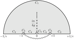
Figure 4: Contour $C$ and its decomposition (C).

Let us first consider the integral over the large semicircle $C_{1}$. Here we have

$$f(z)=\frac{1}{4}+\mathcal{O}(1/z)$$ (C.6)

and for large enough $1/\epsilon$ we find (neglecting corrections in $\epsilon$)

$$8\pi g^{2}\int_{C_{1}}\frac{dz\,f(z)}{\sinh^{2}(4\pi gz)}=2\pi g^{2}\int_{C_{1}}\frac{dz}{\sinh^{2}(4\pi gz)}=g\coth(4\pi g/\epsilon)=g=c^{(0)}_{2,3}\,g.$$ (C.7)

The first term in $f(z)$ leads to no singularity on the real axis and can be integrated straightforwardly over the remaining contours

$$\lim_{m\to\infty}\int_{C_{2}\cup C_{3}\cup C_{4}\cup C_{5}}\frac{16\pi g^{2}\,dz\,z^{2}}{\sinh^{2}(4\pi gz)}=\int_{-\infty}^{\infty}\frac{16\pi g^{2}\,dz\,z^{2}}{\sinh^{2}(4\pi gz)}=\frac{1}{12g}=\frac{c^{(2)}_{2,3}}{g}\,.$$ (C.8)

For very small $z$ the remaining hypergeometric function goes as

$$\mathop{{}_{2}\smash{\operator@font F}_{1}\vphantom{a}}\nolimits(-{\textstyle\frac{1}{2}},{\textstyle\frac{1}{2}};2;z^{-2})\sim\frac{4i}{3\pi z}$$ (C.9)

so that the semi-circle $C_{5}$ at the origin contributes

$$-\int_{C_{5}}\frac{16\pi g^{2}\,dz\,z^{2}}{\sinh^{2}(4\pi gz)}\mathop{{}_{2}\smash{\operator@font F}_{1}\vphantom{a}}\nolimits(-{\textstyle\frac{1}{2}},{\textstyle\frac{1}{2}};2;z^{-2})=-\frac{4}{3\pi}=c_{2,3}^{(1)}\,.$$ (C.10)

Since the integrand is an even function of $z$, the other three pieces add up to the real part of an integral along the positive semi-axis only:

$$H(g)\mathrel{} = \mathrel{}-16\pi g^{2}\int_{C_{2}\cup C_{3}\cup C_{4}}\frac{dz\,z^{2}}{\sinh^{2}(4\pi gz)}\,\mathop{{}_{2}\smash{\operator@font F}_{1}\vphantom{a}}\nolimits(-{\textstyle\frac{1}{2}},{\textstyle\frac{1}{2}};2;z^{-2})$$ (C.11)

$$= \mathrel{}-32\pi g^{2}\,\mathop{\operator@font Re}\nolimits\int_{0}^{\infty}\frac{dz\,z^{2}}{\sinh^{2}(4\pi gz)}\,\mathop{{}_{2}\smash{\operator@font F}_{1}\vphantom{a}}\nolimits(-{\textstyle\frac{1}{2}},{\textstyle\frac{1}{2}};2;z^{-2})$$

The real part of the hypergeometric function is easily read off from its one-parameter representation

$$\mathop{\operator@font Re}\nolimits\mathop{{}_{2}\smash{\operator@font F}_{1}\vphantom{a}}\nolimits(-{\textstyle\frac{1}{2}},{\textstyle\frac{1}{2}};2;z^{-2})=\frac{4}{\pi}\int_{0}^{\min(z,1)}dt\,\sqrt{1-t^{2}}\sqrt{1-t^{2}z^{-2}}\,.$$ (C.12)

In $H(g)$ we readily estimate the contribution from $z>1$ to be of order $\mathcal{O}(e^{-g})$ due to the suppression by $1/\sinh(4\pi gz)^{2}$. The remainder is

$$H(g)=-128g^{2}\int_{0}^{1}\frac{dz\,z^{2}}{\sinh^{2}(4\pi gz)}\int_{0}^{z}dt\,\sqrt{1-t^{2}}\sqrt{1-t^{2}z^{-2}}+\mathcal{O}(e^{-g})\,.$$ (C.13)

To deal with these integrals we successively

• expand $\sqrt{1-t^{2}}$ into a series in $t$

  $$\sqrt{1-t^{2}}=-\frac{1}{2\sqrt{\pi}}\sum_{m=0}^{\infty}\frac{\mathop{\smash{\Gamma}\vphantom{a}}\nolimits(m-\frac{1}{2})}{\mathop{\smash{\Gamma}\vphantom{a}}\nolimits(m+1)}\,t^{2n},$$ (C.14)

• calculate the $t$ integral in each term

  $$\int_{0}^{z}dt\,t^{2m}\sqrt{1-t^{2}z^{-2}}=\frac{\sqrt{\pi}}{4}\,\frac{\mathop{\smash{\Gamma}\vphantom{a}}\nolimits(m+{\textstyle\frac{1}{2}})}{\mathop{\smash{\Gamma}\vphantom{a}}\nolimits(m+2)}\,z^{1+2m},$$ (C.15)

• evaluate the $z$ integral. Here we may extend the range to the whole positive semi-axis since the error is again seen to be $\mathcal{O}(e^{-g})$

  $$\int_{0}^{1}\frac{dz\,z^{2m+3}}{\sinh^{2}(4\pi gz)}=\int_{0}^{\infty}\frac{dz\,z^{2m+3}}{\sinh^{2}(4\pi gz)}+\mathcal{O}(e^{-g})=\frac{4\mathop{\smash{\Gamma}\vphantom{a}}\nolimits(2m+4)\,\zeta(2m+3)}{(8\pi g)^{2m+4}}+\mathcal{O}(e^{-g}).$$ (C.16)

On collecting terms:

$$H(g)\mathrel{} = \mathrel{}\sum_{m=0}^{\infty}\frac{\mathop{\smash{\Gamma}\vphantom{a}}\nolimits(m-\frac{1}{2})\mathop{\smash{\Gamma}\vphantom{a}}\nolimits(m+\frac{1}{2})\mathop{\smash{\Gamma}\vphantom{a}}\nolimits(2m+4)}{\mathop{\smash{\Gamma}\vphantom{a}}\nolimits(m+1)\mathop{\smash{\Gamma}\vphantom{a}}\nolimits(m+2)}\,\frac{\zeta(2m+3)}{\pi^{2}(8\pi g)^{2m+2}}+\mathcal{O}(e^{-g})$$ (C.17)

$$= \mathrel{}\sum_{n=3}^{\infty}\frac{2\,\zeta(n)}{(-2\pi)^{n}\mathop{\smash{\Gamma}\vphantom{a}}\nolimits(n-1)}\,\frac{\mathop{\smash{\Gamma}\vphantom{a}}\nolimits[\frac{1}{2}(n+2)]\mathop{\smash{\Gamma}\vphantom{a}}\nolimits[\frac{1}{2}n]}{\mathop{\smash{\Gamma}\vphantom{a}}\nolimits[\frac{1}{2}(6-n)]\mathop{\smash{\Gamma}\vphantom{a}}\nolimits[\frac{1}{2}(4-n)]}\,g^{1-n}+\mathcal{O}(e^{-g})$$

$$= \mathrel{}\sum_{n=3}^{\infty}c_{2,3}^{(n)}\,g^{1-n}+\mathcal{O}(e^{-g})\,.$$

The second line is obtained by using some identities of gamma functions and setting $n=2m+3$. In conclusion:

$$c_{2,3}(g)=c_{2,3}^{(0)}\,g+c_{2,3}^{(1)}+\frac{c^{(2)}_{2,3}}{g}+H(g)=\sum_{m=0}^{\infty}c_{2,3}^{(m)}g^{1-m}+\mathcal{O}(e^{-g}).$$ (C.18)

We proved the correctness of the strong-coupling expansion coefficients $c_{r,s}^{(m)}$ from equation (3.4) (see also (3.23)) for the case $(r,s)=(2,3)$. The role of the zeta function regularisation used in the main text is simply to dispose of the terms of order $\mathcal{O}(e^{-g})$ that become visible in this proof.

The argument presented in this appendix should remain applicable for generic values of $(r,s)$. We hope to return to this general case in future work. We can however perform the analysis for the first two orders. By Euler-MacLaurin summation (or zeta function regularization), the leading two orders of $c_{r,s}(g)$ takes the form

$$c^{(0)}_{r,s}=\int_{0}^{\infty}h_{r,s}(1/z)\,dz,\qquad c^{(1)}_{r,s}=\zeta(0)h_{r,s}(\infty).$$ (C.19)

In fact, one can show that the above argument yields the same answers. The integral of $h_{r,s}$ in the form (3.25) can be performed in closed form for all $(r,s)$

$$c^{(0)}_{r,s}=\frac{8(r-1)(s-1)\sin[\pi(r-s)]}{\pi(s-r-1)(s-r+1)(s+r-3)(s+r-1)}=\delta_{r+1,s}$$ (C.20)

and one obtains full agreement with the AFS phase (3.5) [25] using that $r,s$ are integers with $r\geq s+1$. For the next order one can use the representation (A.10) of $h_{r,s}(z)$ at $z=\infty$

$$c^{(1)}_{r,s}\mathrel{} = \mathrel{}\zeta(0)2\cos[{\textstyle\frac{1}{2}}\pi(s-r-1)]\,(r-1)(s-1)\int_{0}^{\infty}\frac{dt}{t}\,\mathop{\smash{J_{r-1}}\vphantom{a_{r-1}}}\nolimits(2\,t)\mathop{\smash{J_{s-1}}\vphantom{a_{s-1}}}\nolimits(2\,t)$$ (C.21)

$$= \mathrel{}-\cos[{\textstyle\frac{1}{2}}\pi(s-r-1)](r-1)(s-1)\frac{2\cos[{\textstyle\frac{1}{2}}\pi(s-r-1)]}{\pi(s-r)(s+r-2)}$$

$$= \mathrel{}-\frac{1-(-1)^{r+s}}{\pi}\,\frac{(r-1)(s-1)}{(s-r)(s+r-2)}\,.$$

This is again in full agreement with the HL phase (3.5) [41].

References

- [1] M. Staudacher, “The factorized S-matrix of CFT/AdS”, JHEP 0505, 054 (2005), hep-th/0412188.
- [2] D. Berenstein, J. M. Maldacena and H. Nastase, “Strings in flat space and pp waves from 4 Super Yang Mills”, JHEP 0204, 013 (2002), hep-th/0202021.
- [3] J. A. Minahan and K. Zarembo, “The Bethe-ansatz for 4 super Yang-Mills”, JHEP 0303, 013 (2003), hep-th/0212208.
- [4] N. Beisert and M. Staudacher, “The 4 SYM Integrable Super Spin Chain”, Nucl. Phys. B670, 439 (2003), hep-th/0307042.
- [5] N. Beisert, C. Kristjansen and M. Staudacher, “The Dilatation Operator of 4 Conformal Super Yang-Mills Theory”, Nucl. Phys. B664, 131 (2003), hep-th/0303060.
- [6] N. Beisert, “The SU(22) Dynamic S-Matrix”, hep-th/0511082.
- [7] N. Beisert and M. Staudacher, “Long-Range PSU(2,24) Bethe Ansaetze for Gauge Theory and Strings”, Nucl. Phys. B727, 1 (2005), hep-th/0504190.
- [8] C. Anastasiou, Z. Bern, L. J. Dixon and D. A. Kosower, “Planar amplitudes in maximally supersymmetric Yang-Mills theory”, Phys. Rev. Lett. 91, 251602 (2003), hep-th/0309040.
- [9] Z. Bern, L. J. Dixon and V. A. Smirnov, “Iteration of planar amplitudes in maximally supersymmetric Yang-Mills theory at three loops and beyond”, Phys. Rev. D72, 085001 (2005), hep-th/0505205.
- [10] G. Sterman and M. E. Tejeda-Yeomans, “Multi-loop amplitudes and resummation”, Phys. Lett. B552, 48 (2003), hep-ph/0210130.
- [11] A. V. Kotikov, L. N. Lipatov, A. I. Onishchenko and V. N. Velizhanin, “Three-loop universal anomalous dimension of the Wilson operators in 4 SUSY Yang-Mills model”, Phys. Lett. B595, 521 (2004), hep-th/0404092.
- [12] S. Moch, J. A. M. Vermaseren and A. Vogt, “The three-loop splitting functions in QCD: The non-singlet case”, Nucl. Phys. B688, 101 (2004), hep-ph/0403192.
- [13] Z. Bern, “The S-Matrix Reloaded: Twistors, Unitarity, Gauge Theories and Gravity”, Talk at Workshop on Integrability in Gauge and String Theory, AEI, Potsdam, Germany, July 24-28, 2006, http://int06.aei.mpg.de/presentations/bern.pdf.
- [14] D. A. Kosower, “On-Shell Methods in Field Theory”, Talk at Workshop on Integrability in Gauge and String Theory, AEI, Potsdam, Germany, July 24-28, 2006, http://int06.aei.mpg.de/presentations/kosower.pdf.
- [15] Z. Bern, M. Czakon, L. J. Dixon, D. A. Kosower and V. A. Smirnov, “The Four-Loop Planar Amplitude and Cusp Anomalous Dimension in Maximally Supersymmetric Yang-Mills Theory”, hep-th/0610248.
- [16] B. Eden and M. Staudacher, “Integrability and transcendentality”, hep-th/0603157.
- [17] A. V. Kotikov and L. N. Lipatov, “DGLAP and BFKL equations in the 4 supersymmetric gauge theory”, Nucl. Phys. B661, 19 (2003), hep-ph/0208220.
- [18] C. G. Callan, Jr., H. K. Lee, T. McLoughlin, J. H. Schwarz, I. Swanson and X. Wu, “Quantizing string theory in : Beyond the pp-wave”, Nucl. Phys. B673, 3 (2003), hep-th/0307032.
- [19] D. Serban and M. Staudacher, “Planar 4 gauge theory and the Inozemtsev long range spin chain”, JHEP 0406, 001 (2004), hep-th/0401057.
- [20] J. M. Maldacena, “The large N limit of superconformal field theories and supergravity”, Adv. Theor. Math. Phys. 2, 231 (1998), hep-th/9711200.
- [21] S. S. Gubser, I. R. Klebanov and A. M. Polyakov, “Gauge theory correlators from non-critical string theory”, Phys. Lett. B428, 105 (1998), hep-th/9802109.
- [22] E. Witten, “Anti-de Sitter space and holography”, Adv. Theor. Math. Phys. 2, 253 (1998), hep-th/9802150.
- [23] D. M. Hofman and J. M. Maldacena, “Giant magnons”, J. Phys. A39, 13095 (2006), hep-th/0604135.
- [24] G. Arutyunov, S. Frolov, J. Plefka and M. Zamaklar, “The Off-shell Symmetry Algebra of the Light-cone Superstring”, hep-th/0609157.
- [25] G. Arutyunov, S. Frolov and M. Staudacher, “Bethe ansatz for quantum strings”, JHEP 0410, 016 (2004), hep-th/0406256.
- [26] V. A. Kazakov, A. Marshakov, J. A. Minahan and K. Zarembo, “Classical/quantum integrability in AdS/CFT”, JHEP 0405, 024 (2004), hep-th/0402207.
- [27] R. A. Janik, “The superstring worldsheet S-matrix and crossing symmetry”, Phys. Rev. D73, 086006 (2006), hep-th/0603038.
- [28] G. Arutyunov and S. Frolov, “On string S-matrix”, Phys. Lett. B639, 378 (2006), hep-th/0604043.
- [29] N. Beisert, R. Hernández and E. López, “A Crossing-Symmetric Phase for Strings”, hep-th/0609044.
- [30] N. Beisert and T. Klose, “Long-Range Integrable Spin Chains and Plane-Wave Matrix Theory”, J. Stat. Mech. 06, P07006 (2006), hep-th/0510124.
- [31] B. Eden, “A two-loop test for the factorised S-matrix of planar 4”, Nucl. Phys. B738, 409 (2006), hep-th/0501234.
- [32] B. I. Zwiebel, “4 SYM to two loops: Compact expressions for the non-compact symmetry algebra of the su(1,12) sector”, JHEP 0602, 055 (2006), hep-th/0511109.
- [33] N. Beisert, V. Dippel and M. Staudacher, “A Novel Long Range Spin Chain and Planar 4 Super Yang-Mills”, JHEP 0407, 075 (2004), hep-th/0405001.
- [34] A. V. Belitsky, A. S. Gorsky and G. P. Korchemsky, “Logarithmic scaling in gauge / string correspondence”, Nucl. Phys. B748, 24 (2006), hep-th/0601112.
- [35] G. P. Korchemsky, “Quasiclassical QCD pomeron”, Nucl. Phys. B462, 333 (1996), hep-th/9508025.
- [36] L. N. Lipatov, “Transcendentality and Eden-Staudacher equation”, Talk at Workshop on Integrability in Gauge and String Theory, AEI, Potsdam, Germany, July 24-28, 2006, http://int06.aei.mpg.de/presentations/lipatov.pdf.
- [37] N. Beisert, “The SU(23) Dynamic Spin Chain”, Nucl. Phys. B682, 487 (2004), hep-th/0310252.
- [38] B. Eden, C. Jarczak and E. Sokatchev, “A three-loop test of the dilatation operator in 4 SYM”, Nucl. Phys. B712, 157 (2005), hep-th/0409009.
- [39] M. Staudacher, unpublished.
- [40] N. Beisert and A. A. Tseytlin, “On Quantum Corrections to Spinning Strings and Bethe Equations”, Phys. Lett. B629, 102 (2005), hep-th/0509084.
- [41] R. Hernández and E. López, “Quantum corrections to the string Bethe ansatz”, JHEP 0607, 004 (2006), hep-th/0603204.
- [42] L. Freyhult and C. Kristjansen, “A universality test of the quantum string Bethe ansatz”, Phys. Lett. B638, 258 (2006), hep-th/0604069.
- [43] N. Beisert, unpublished.
- [44] G. Arutyunov, J. Plefka and M. Staudacher, “Limiting geometries of two circular Maldacena-Wilson loop operators”, JHEP 0112, 014 (2001), hep-th/0111290.
- [45] J. Maldacena, “Wilson loops in large N field theories”, Phys. Rev. Lett. 80, 4859 (1998), hep-th/9803002.
- [46] J. K. Erickson, G. W. Semenoff and K. Zarembo, “Wilson loops in 4 supersymmetric Yang-Mills theory”, Nucl. Phys. B582, 155 (2000), hep-th/0003055.
- [47] N. Drukker and D. J. Gross, “An exact prediction of 4 SUSYM theory for string theory”, J. Math. Phys. 42, 2896 (2001), hep-th/0010274.
- [48] R. Celorrio and F.-J. Sayas, “The Euler-MacLaurin formula in presence of a logarithmic singularity”, BIT 39, 780 (1998).
- [49] N. Dorey, “Magnon bound states and the AdS/CFT correspondence”, J. Phys. A39, 13119 (2006), hep-th/0604175.
- [50] H.-Y. Chen, N. Dorey and K. Okamura, “On the scattering of magnon boundstates”, hep-th/0608047.
- [51] R. Roiban, “Magnon bound-state scattering in gauge and string theory”, hep-th/0608049.
- [52] N. Beisert, “The Analytic Bethe Ansatz for a Chain with Centrally Extended su(22) Symmetry”, nlin.SI/0610017.
- [53] S. S. Gubser, I. R. Klebanov and A. M. Polyakov, “A semi-classical limit of the gauge/string correspondence”, Nucl. Phys. B636, 99 (2002), hep-th/0204051.
- [54] S. Frolov and A. A. Tseytlin, “Semiclassical quantization of rotating superstring in ”, JHEP 0206, 007 (2002), hep-th/0204226.
- [55] S. Frolov and M. Staudacher, work in progress.
- [56] A. V. Kotikov, L. N. Lipatov and V. N. Velizhanin, “Anomalous dimensions of Wilson operators in 4 SYM theory”, Phys. Lett. B557, 114 (2003), hep-ph/0301021.
- [57] A. Rej, D. Serban and M. Staudacher, “Planar 4 Gauge Theory and the Hubbard Model”, JHEP 0603, 018 (2006), hep-th/0512077.
- [58] S. Schäfer-Nameki, M. Zamaklar and K. Zarembo, “Quantum corrections to spinning strings in and Bethe ansatz: A comparative study”, JHEP 0509, 051 (2005), hep-th/0507189.
- [59] S. Schäfer-Nameki, M. Zamaklar and K. Zarembo, “How Accurate is the Quantum String Bethe Ansatz?”, hep-th/0610250.
- [60] N. Mann and J. Polchinski, “Bethe ansatz for a quantum supercoset sigma model”, Phys. Rev. D72, 086002 (2005), hep-th/0508232.
- [61] N. Gromov, V. Kazakov, K. Sakai and P. Vieira, “Strings as multi-particle states of quantum sigma-models”, hep-th/0603043.
- [62] N. Gromov and V. Kazakov, “Asymptotic Bethe ansatz from string sigma model on ”, hep-th/0605026.
- [63] J. Ambjørn, R. A. Janik and C. Kristjansen, “Wrapping interactions and a new source of corrections to the spin-chain / string duality”, Nucl. Phys. B736, 288 (2006), hep-th/0510171.
- [64] J. Teschner, “The Sinh-Gordon Model — A Warm-Up for Noncompact Nonlinear Sigma Models?”, Talk at Workshop on Integrability in Gauge and String Theory, AEI, Potsdam, Germany, July 24-28, 2006, http://int06.aei.mpg.de/presentations/teschner.pdf.
- [65] A. G. Bytsko and J. Teschner, “Quantization of models with non-compact quantum group symmetry: Modular XXZ magnet and lattice sinh-Gordon model”, J. Phys. A39, 12927 (2006), hep-th/0602093.
- [66] I. R. Klebanov, M. Spradlin and A. Volovich, “New effects in gauge theory from pp-wave superstrings”, Phys. Lett. B548, 111 (2002), hep-th/0206221.
- [67] N. Beisert, “Higher-Loop Integrability in 4 Gauge Theory”, Comptes Rendus Physique 5, 1039 (2004), hep-th/0409147.
- [68] I. Klebanov, “Strings, D-Branes and Gauge Theories”, Talk at Workshop on Integrability in Gauge and String Theory, AEI, Potsdam, Germany, July 24-28, 2006, http://int06.aei.mpg.de/presentations/klebanov.pdf.
- [69] M. Staudacher, “Integrability, Transcendentality, and the AdS/CFT Correspondence”, Talk at Workshop on Integrability in Gauge and String Theory, AEI, Potsdam, Germany, July 24-28, 2006, http://int06.aei.mpg.de/presentations/staudacher.pdf.
- [70] D. J. Gross, A. Mikhailov and R. Roiban, “Operators with large R charge in 4 Yang-Mills theory”, Annals Phys. 301, 31 (2002), hep-th/0205066.
- [71] A. Santambrogio and D. Zanon, “Exact anomalous dimensions of 4 Yang-Mills operators with large R charge”, Phys. Lett. B545, 425 (2002), hep-th/0206079.
- [72] S. Frolov and A. A. Tseytlin, “Multi-spin string solutions in ”, Nucl. Phys. B668, 77 (2003), hep-th/0304255.
- [73] N. Beisert, J. A. Minahan, M. Staudacher and K. Zarembo, “Stringing Spins and Spinning Strings”, JHEP 0309, 010 (2003), hep-th/0306139.
- [74] T. Fischbacher, T. Klose and J. Plefka, “Planar plane-wave matrix theory at the four loop order: Integrability without BMN scaling”, JHEP 0502, 039 (2005), hep-th/0412331.
- [75] D. Serban, unpublished.
- [76] E. N. Economou and P. N. Poulopoulos, “Ground-state energy of the half-filled one-dimensional Hubbard model”, Phys. Rev. B20, 4756 (1979).