hep-th/0610250
AEI-2006-081
CALT-68-2613
ITEP-TH-52/06
UUITP-14/06

We compare solutions of the quantum string Bethe equations with explicit one-loop calculations in the sigma-model on $AdS_{5}\times S^{5}$. The Bethe ansatz exactly reproduces the spectrum of infinitely long strings. When the length is finite, we find that deviations from the exact answer arise which are exponentially small in the string length.

1 Introduction

The string sigma-model in $AdS_{5}\times S^{5}$ [1] is integrable [2] and is presumably solvable by means of a Bethe ansatz [3, 4, 5, 6]. Ultimately we want to understand closed strings with periodic boundary conditions over a finite range of the world-sheet coordinate. This is not an easy task from the Bethe ansatz perspective. It is usually simpler to solve the theory on an infinite line, when one can define asymptotic states and use bootstrap to find the scattering matrix [7]. The diagonalization of the S-matrix then determines the spectrum via the asymptotic Bethe equations. Such Bethe equations are approximate for a system of finite size. They do not capture effects of vacuum polarization by particles that travel around the circle [8]. Circumventing this problem is in principle possible, but requires the use of more complicated algebraic techniques [9].

The currently known Bethe equations for quantum strings in $AdS_{5}\times S^{5}$ [4, 6] are of this asymptotic type. They are determined by the S-matrix [10] and would have a chance to be exact only if interactions on the world-sheet were ultra local, which is not the case: the scattering states are arguably solitons of finite size (giant magnons) [11] and we also expect that bare point-like interactions are smeared over a finite range by vacuum polarization. This Casimir-type effect is expected to produce exponential corrections to the energy levels in the large-volume limit [8]. Exponential terms were indeed seen in the one-loop energy shifts for macroscopic spinning strings [12, 13] and in the dispersion relation of a single giant magnon [14].

Our goal is to understand how good an approximation the asymptotic Bethe ansatz for strings of finite length is. To do that we shall study quantum corrections to a specific class of spinning string solutions described in appendix A. One-loop corrections to these solution are known [15] and were compared to the predictions of the Bethe ansatz in our previous paper [16]. The discrepancies found there were finite rather than exponential. It was later realized that the Bethe equations themselves are modified by quantum effects [17]. The one-loop correction factor was found in [18] and we will update our calculation to take this factor into account.

In string theory, the range of the world-sheet coordinate is a gauge-dependent quantity. It should not be confused with the proper size of the string in the target space, which can be very small even for strings with infinite world-volume. However, in any physical gauge (light-cone, temporal, or the like) the internal length of the string is naturally identified with the target-space momentum measured in the units of $\alpha^{\prime}$ [19]: The string grows in size when the momentum becomes large [20]. For the states that we shall consider the length is $2\pi\mathcal{J}=2\pi J/\sqrt{\lambda}$, where $J$ is the angular momentum on $S^{5}$ (dual to the R-charge in $\mathcal{N}=4$ super-Yang-Mills theory) and $\lambda=g_{\rm YM}^{2}N$ is the SYM ’t Hooft coupling. In the decompactification limit $\mathcal{J}\rightarrow\infty$, one is left with the sigma model on a line with the coupling constant $2\pi/\sqrt{\lambda}$. $1/\sqrt{\lambda}$ plays the role of the loop counting parameter in the sigma-model. The usual perturbation theory then yields a power series in $1/\sqrt{\lambda}$ for the energy spectrum: $E=\sqrt{\lambda}\,\mathcal{E}+\delta E+\ldots$.

2 Finite-size corrections

The energy, as a function of the string length, can be expanded at $\mathcal{J}\gg 1$ as [17, 12, 8, 13]

$$\delta E=\sum_{l=2}^{\infty}\frac{f_{l}}{\mathcal{J}^{l}}+\sum_{s=0}^{\infty}a_{s}\,{\rm e}\,^{-2\pi s\mathcal{J}}\,.$$ (2.1)

It is known that the string Bethe ansatz reproduces all orders in $1/\mathcal{J}$ (all $f_{l}$’s) exactly [16, 17]. For the reasons explained in the introduction we expect exponential corrections to also arise.

To see how that happens, let us begin with a simple example: the zero-point energy of $N$ massive bosons and fermions in two dimensions with twisted boundary conditions

$$\mathcal{F}\left(\mu_{i}\right)=\frac{1}{2}\sum_{n=-\infty}^{+\infty}\sum_{i=1}^{N}\left(-1\right)^{F_{i}}\sqrt{\left(n+\gamma_{i}\right)^{2}+\mu_{i}^{2}}-\frac{1}{2}\sum_{i=1}^{N}\left(-1\right)^{F_{i}}\gamma_{i}^{2}.$$ (2.2)

The sum converges if

$$\sum_{i}\left(-1\right)^{F_{i}}=0,\qquad\sum_{i}\left(-1\right)^{F_{i}}\mu_{i}^{2}=0.$$ (2.3)

In addition, the summation should be performed symmetrically in $n\rightarrow-n$ if any of the $\gamma_{i}$’s is non-zero. In what follows we will only encounter the periodic boundary conditions, which correspond to all $\gamma_{i}=0$, in which case we denote the zero-point energy by $\mathcal{F}_{p}$. But it is instructive to consider a more general twisted sum (2.2).

The parameters $\mu_{i}$ in (2.2) are masses measured in the units of length: $\mu_{i}=m_{i}L/2\pi$. Hence the large-volume limit is $\mu_{i}\rightarrow\infty$. The summation over mode numbers can then be replaced by momentum integration to a first approximation:

$$\mathcal{F}\approx\frac{1}{2}\int_{-\infty}^{+\infty}dp\,\sum_{i}\left(-1\right)^{F_{i}}\sqrt{\left(p+\gamma_{i}\right)^{2}+\mu_{i}^{2}}-\frac{1}{2}\sum_{i}\left(-1\right)^{F_{i}}\gamma_{i}^{2}=-\frac{1}{2}\sum_{i}\left(-1\right)^{F_{i}}\mu_{i}^{2}\ln\mu_{i}.$$ (2.4)

As expected, the macroscopic part of the zero-point energy does not depend on the boundary conditions.

The approximate expression (2.4) is obviously exact only in the infinite-volume limit. The finite-size corrections can be taken into account by Poisson resummation

$$\mathcal{F}=\frac{1}{2}\sum_{s=-\infty}^{+\infty}\int_{-\infty}^{+\infty}dp\,\,{\rm e}\,^{2\pi ips}\sum_{i}\left(-1\right)^{F_{i}}\sqrt{\left(p+\gamma_{i}\right)^{2}+\mu_{i}^{2}}-\frac{1}{2}\sum_{i}\left(-1\right)^{F_{i}}\gamma_{i}^{2},$$ (2.5)

which yields

$$\mathcal{F}=-\frac{1}{2}\sum_{i}\left(-1\right)^{F_{i}}\mu_{i}^{2}\ln\mu_{i}-\sum_{s=1}^{\infty}\frac{1}{\pi s}\sum_{i}\left(-1\right)^{F_{i}}\cos(2\pi s\gamma_{i})\mu_{i}K_{1}(2\pi s\mu_{i}).$$ (2.6)

In the case of periodic boundary conditions this becomes

$$\mathcal{F}_{p}=-\frac{1}{2}\sum_{i}\left(-1\right)^{F_{i}}\mu_{i}^{2}\ln\mu_{i}-\sum_{s=1}^{\infty}\frac{1}{\pi s}\sum_{i}\left(-1\right)^{F_{i}}\mu_{i}K_{1}(2\pi s\mu_{i}).$$ (2.7)

Since the modified Bessel function behaves at large values of the argument as

$$K_{1}(x)\approx\sqrt{\frac{\pi}{2x}}\,\,{\rm e}\,^{-x},$$ (2.8)

the finite-volume corrections are exponential as long as all modes are massive.

3 Semi-classical strings

The one-loop energy shift for any rigid-string solution is given by the sum over frequencies of fluctuation modes

$$\delta E=\frac{1}{2}\sum_{n}\left(-1\right)^{F_{n}}\omega_{n}.$$ (3.1)

We consider a specific class of solutions which are characterized by angular momentum $J$ and winding number $m$ on $S^{5}$ and by spin $S$ and winding number $k$ in $AdS_{5}$. The parameters of the solution are related by

$$kS+mJ=0.$$ (3.2)

One of the winding numbers must be negative, and for definiteness we choose $m>0$ and $k<0$. The explicit form of the solution is described in Appendix A.

The frequencies of normal modes for this solution were computed in [15] and are rather complicated functions of $\mathcal{J}=J/\sqrt{\lambda}$ and $\mathcal{S}=S/\sqrt{\lambda}$. Half of the bosonic frequencies is known only implicitly as the roots of a particular fourth-order polynomial. In order to proceed we make a further simplifying assumption. Namely, we consider the limit

$$k\rightarrow\infty\,,\qquad\quad\mathcal{S}\rightarrow 0\,,\qquad\quad\mathcal{J},\,m{~{}-~{}\rm finite}\,$$ (3.3)

and systematically drop $O(1/k)$ corrections. The solution considerably simplifies in this limit. The sum over frequencies reduces to the free-field expression considered in the previous section

$$E = J+\sqrt{\lambda}\,m+\frac{4\mathcal{F}_{p}\left(\sqrt{\mathcal{J}^{2}-m^{2}},\mathcal{J}+m;\sqrt{\mathcal{J}(\mathcal{J}+m)},\sqrt{\mathcal{J}(\mathcal{J}+m)}\right)}{\mathcal{J}+m}$$ (3.4)

$$+\sqrt{\mathcal{J}m}-m+\left(\mathcal{J}+m\right)\ln\frac{\sqrt{\mathcal{J}+m}}{\sqrt{\mathcal{J}}+\sqrt{m}}\,.$$

The first two terms represent the classical, $O(\sqrt{\lambda})$ energy of the spinning string. The rest is the $O(1)$ one-loop quantum correction $\delta E$. The spectrum consists of eight degenerate fermions with mass $\sqrt{\mathcal{J}(\mathcal{J}+m)}$, four bosons with mass $\sqrt{\mathcal{J}^{2}-m^{2}}$, and four bosons with mass $\mathcal{J}+m$, and satisfies the convergence conditions (2.3).

Using (2.7) and (2.8) we find that at large $\mathcal{J}$ the one-loop correction to the energy indeed has the form (2.1):

$$\delta E^{\rm string} = \sqrt{\mathcal{J}m}-m+\mathcal{J}\ln\frac{\mathcal{J}^{2}}{\sqrt{\mathcal{J}+m}\left(\sqrt{\mathcal{J}}+\sqrt{m}\right)\left(\mathcal{J}-m\right)}+m\ln\frac{\sqrt{\mathcal{J}}-\sqrt{m}}{\sqrt{\mathcal{J}+m}}$$ (3.5)

$$-\frac{2\left(1-\,{\rm e}\,^{-\pi m}\right)^{2}}{\pi\sqrt{\mathcal{J}}}\,\,{\rm e}\,^{-2\pi\mathcal{J}}+\ldots.$$

The first line is the infinite-length limit of the string quantum correction. It is obtained by replacing the sum over the string modes by the momentum integral. The exponential term can be extracted from the first Bessel function in (2.7).

4 Quantum string Bethe ansatz

The solution we consider belongs to the $sl(2)$ sector, Bethe equations for which read [5, 6]

$$\left(\frac{x_{k}^{+}}{x_{k}^{-}}\right)^{J}=\prod_{j\neq k}\frac{x_{k}^{-}-x_{j}^{+}}{x_{k}^{+}-x_{j}^{-}}\,\,\frac{1-\frac{1}{x_{k}^{+}x_{j}^{-}}}{1-\frac{1}{x_{k}^{-}x_{j}^{+}}}\,\,{\rm e}\,^{i\theta(x_{k},x_{j})}.$$ (4.1)

The state with spin $S$ is characterized by $S$ Bethe roots $x_{k}$. All Bethe roots are real. $x_{k}^{\pm}$ are defined by

$$x^{\pm}+\frac{1}{x^{\pm}}=x+\frac{1}{x}\pm\frac{2\pi i}{\sqrt{\lambda}}\,.$$ (4.2)

The Bethe equations contain a dressing phase of the following general form [4]

$$\theta(x_{k},x_{j})=\frac{1}{\pi}\sum_{r,s=\pm}rs\left(\chi(x^{r}_{k},x^{s}_{j})-\chi(x^{r}_{j},x^{s}_{k})\right),$$ (4.3)

where the function $\chi(x,y)$ is defined as power series

$$\chi(x,y)=-\frac{\sqrt{\lambda}}{2}\sum_{r=2}^{\infty}\sum_{n=0}^{\infty}\frac{c_{r,n}}{\left(r-1\right)\left(r+2n\right)}\,\,\frac{1}{x^{r-1}y^{r+2n}}$$ (4.4)

The coefficients $c_{r,n}$ are known to the first two orders in $1/\sqrt{\lambda}$ [4, 18, 23]

$$c_{r,n}=\delta_{n\,0}-\frac{8}{\sqrt{\lambda}}\,\,\frac{\left(r-1\right)\left(r+2n\right)}{\left(2r+2n-1\right)\left(2n+1\right)}\,.$$ (4.5)

The one-loop term was proposed in [18] and passes a number of consistency tests: it is universal for all sectors [24], and it satisfies [25] the crossing-symmetry relation [26].

In the scaling limit of large $J$, $S$, and $\lambda$, the number of Bethe roots goes to infinity, but each $x_{k}$ remains finite. The distance between $x_{k}$ and $x_{k+1}$, however, goes to zero as $1/\sqrt{\lambda}$, so that the Bethe roots form a continuous distribution, which can be characterized by the density

$$\rho(x)=\frac{4\pi}{\sqrt{\lambda}}\sum_{k=1}^{S}\frac{x_{k}^{2}}{x_{k}^{2}-1}\,\delta(x-x_{k}),$$ (4.6)

or by the resolvent

$$G(z)=\frac{4\pi}{\sqrt{\lambda}}\sum_{k=1}^{S}\frac{x_{k}^{2}}{x_{k}^{2}-1}\,\,\frac{1}{z-x_{k}}=\int dx\,\,\frac{\rho(x)}{z-x}\,.$$ (4.7)

In the scaling limit, the Bethe equations reduce to an integral equation for the density or, for the simplest class of solutions that we consider here, to an algebraic equation for the resolvent. These classical Bethe equations can be derived from the equations of motion of the string, and encode all information about periodic solutions of the sigma-model [3]. The discreteness of the quantum Bethe equations leads to an anomalous order $1/\sqrt{\lambda}$ correction to the classical equations [27]. The anomaly contribution was computed in our previous work [16]. Another source of $1/\sqrt{\lambda}$ corrections is the $O(1)$ term in the dressing phase (4.5). Taking both corrections into account we obtain

$$G^{2}(z)-2\pi\left(k-2\,\frac{\mathcal{J}z+m}{z^{2}-1}\right)G(z)++\frac{4\pi^{2}}{z^{2}-1}\left[k(\mathcal{E}+\mathcal{S}-\mathcal{J})z-m(k+m)\right]=\frac{1}{\sqrt{\lambda}}\,\,\frac{z^{2}}{z^{2}-1}V(z).$$ (4.8)

The “external potential” $V(z)$ is calculated in appendix B (eq. (Appendix B Semiclassical Bethe equations )).

Neglecting the right hand side of (4.8) we get the classical solution

$$G_{0}(z)=\pi\left(k-2{\mathcal{J}z+m\over z^{2}-1}\right)+{\pi\sqrt{P(z)}\over z^{2}-1}\,,$$ (4.9)

where

$$P(z)=k^{2}z^{4}-4k(\mathcal{E}+\mathcal{S})z^{3}+2(2\mathcal{J}^{2}+2m^{2}-k^{2})z^{2}+4k(\mathcal{E}-\mathcal{S})z+k^{2}\,.$$ (4.10)

Consistency requires that the polynomial $P(z)$ has a double root

$$P(c)=0,\qquad P^{\prime}(c)=0.$$ (4.11)

The resolvent then is an analytic function on the complex plane with a single cut between two other roots of $P(z)$. The density is defined on this cut and has a typical square-root form: $\rho(x)\sim\sqrt{(b-x)(x-a)}$. The equations (4.11) determine the energy as a function of charges: $\mathcal{E}=\mathcal{E}(\mathcal{J},\mathcal{S})$ in a parametric form. It can be shown that (4.11) are equivalent to (Appendix A The spinning string solution ) [16].

The correction term in (4.8) shifts the energy by $O(\lambda^{0})$. The shift can be calculated from the one-cut consistency condition on the resolvent. The details of the calculation can be found in [16]. Here we just give the result, valid for any external potential $V(z)$:

$$\delta E^{\rm Bethe}=\frac{cV(c)}{4\pi^{2}k}\,.$$ (4.12)

With the explicit form of the potential from (Appendix B Semiclassical Bethe equations ), we get

$$\delta E^{{\rm Bethe}} = \frac{c}{2\pi^{2}k}\int dx\,\,\frac{\rho(x)}{c-x}\,\int dy\,\,\frac{\rho(y)}{c-y}\,\left\{\frac{2}{xy-1}+\left[\frac{x-y}{\left(xy-1\right)^{2}}+\frac{1}{x-y}\right]\ln\frac{\left(x+1\right)\left(y-1\right)}{\left(x-1\right)\left(y+1\right)}\right\}$$ (4.13)

$$-\frac{c}{k}\int dx\,\,\frac{\rho^{\prime}(x)\rho(x)\coth\pi\rho(x)}{c-x}\,.$$

This expression is valid even at finite $k$, but is difficult to handle. Let us now take the large winding limit.

At large $k$ the density is highly peaked at $x\approx-1$, and it is necessary to introduce the rescaled variable $v$:

$$x=-1-\frac{v}{|k|}\,.$$ (4.14)

The parameter $c$ behaves as

$$c=1+O\left(\frac{1}{k}\right)$$ (4.15)

and the density becomes [16]

$$\rho(v)=\frac{|k|}{v}\,\sqrt{2\left(\mathcal{J}+m\right)v-v^{2}-\left(\mathcal{J}-m\right)^{2}}\,.$$ (4.16)

The single integral in (4.13) (the second line) can be done [16]:

$$\delta E^{{\rm Bethe}} = \sqrt{m\mathcal{J}}-\frac{\mathcal{J}+m}{2}\,\ln\frac{\sqrt{\mathcal{J}}+\sqrt{m}}{\sqrt{\mathcal{J}}-\sqrt{m}}+\frac{1}{4\pi^{2}}\int\frac{dv}{v}\,\sqrt{2\left(\mathcal{J}+m\right)v-v^{2}-\left(\mathcal{J}-m\right)^{2}}$$

$$\times\int\frac{dw}{w}\,\sqrt{2\left(\mathcal{J}+m\right)w-w^{2}-\left(\mathcal{J}-m\right)^{2}}\left[\frac{v^{2}+w^{2}}{\left(v+w\right)^{2}\left(v-w\right)}\,\ln\frac{v}{w}-\frac{1}{v+w}\right]\,.$$

The double integral can be also calculated analytically, leading to

$$\delta E^{\rm Bethe}=\sqrt{\mathcal{J}m}-m+\mathcal{J}\ln\frac{\mathcal{J}^{2}}{\sqrt{\mathcal{J}+m}\left(\sqrt{\mathcal{J}}+\sqrt{m}\right)\left(\mathcal{J}-m\right)}+m\ln\frac{\sqrt{\mathcal{J}}-\sqrt{m}}{\sqrt{\mathcal{J}+m}}\,,$$ (4.18)

in which we can recognize the non-exponential part of the exact answer (3.5).

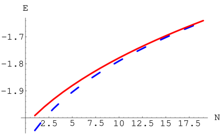
Figure 1: The one-loop correction to the energy as a function of $\mathcal{J}$ for $m=1$ and ${\mathcal{J}}=1+0.1N$. The blue dashed line is the exact string energy (3.4), the red solid line is the Bethe-ansatz result (4.18).

Let us compare (4.18) with the exact energy shift (3.4) numerically. Since the difference is only exponential, it should be numerically small even for $\mathcal{J}\sim 1$. But in our case $\mathcal{J}$ cannot be smaller that $m$. In fact, one of the bosonic modes becomes massless at $\mathcal{J}=m$ , which means that the correction terms in (2.6) cease to be exponentially suppressed. To our surprise, we found that the difference between (4.18) and (3.4) never gets larger that $10\%$ (fig. 1), even very close to the massless limit.

5 Conclusions

We conclude that the Bethe equations (4.1) are asymptotic and describe the string spectrum with an exponential accuracy as long as the string length is sufficiently large. The corrections to the asymptotic energy levels are of order $\exp(-2\pi J/\sqrt{\lambda})$. Similar correction arise at weak coupling due to the wrapping interactions in the SYM [28], which start to affect the energies (anomalous dimensions) at order $\lambda^{J}=\exp(-\ln(1/\lambda)J)$. It would be interesting to understand how the exponent in the finite-size corrections interpolates between $\ln(1/\lambda)$ at $\lambda\rightarrow 0$ and $2\pi/\sqrt{\lambda}$ at $\lambda\rightarrow\infty$.

Can more sophisticated Bethe equations reproduce the exact spectrum of the closed string with periodic boundary conditions? Literature on integrable field theories in finite volume is vast: [29, 9] contains a necessarily incomplete selection of references. Perhaps extra, ”particle” degrees of freedom, such as those in [30, 31], are necessary to correctly account for the finite-size effects. Or maybe one should start from a pseudo-vacuum with all anti-particle levels empty and then carefully fill the Fermi sea in the finite volume [32]. It is not clear to us what could play the role of the Bethe particles on the world-sheet, or how to define the pseudo-vacuum in the AdS string theory, but it would be definitely interesting to repeat the semiclassical calculations of this paper in the context of the truncated models [30, 32] for which these questions have been answered.

Acknowledgements

We would like to thank R. Roiban, J. Teschner and A. Tseytlin for interesting discussions, and to N. Gromov and P. Vieira for pointing out subtleties in boundary conditions for fermionic string modes. The work of K.Z. was supported in part by the Swedish Research Council under contracts 621-2004-3178 and 621-2003-2742, by the Göran Gustafsson Foundation, and by RFBR grant NSh-1999.2003.2 for the support of scientific schools. S.S.N. is supported by a Caltech John A. McCohn Postdoctoral Fellowship in Theoretical Physics.

Appendix A The spinning string solution

Here we briefly review the string configuration we consider. The relevant part of the $AdS_{5}\times S^{5}$ metric in global coordinates is

$$ds^{2}=-\cosh^{2}\rho\,dt^{2}+d\rho^{2}+\sinh^{2}\rho\,d\theta^{2}+d\phi^{2},$$ (A.1)

where the first three terms are the metric of $AdS_{3}$ and $\phi$ is the angle of a big circle in $S^{5}$. The circular string solution [33] has the following form

$$\rho =\,{\rm const}\,, t =\kappa\tau,$$ (A.2)

$$\theta =\sqrt{\kappa^{2}+k^{2}}\,\tau+k\sigma, \phi =\sqrt{\kappa^{2}+m^{2}}\,\tau+m\sigma$$

where

$$r_{1}^{2}\equiv\sinh^{2}\rho = \frac{\mathcal{S}}{\sqrt{\kappa^{2}+k^{2}}}\,,$$

$$\mathcal{E} = \frac{\kappa\mathcal{S}}{\sqrt{\kappa^{2}+k^{2}}}+\kappa\,,$$ (A.3)

and

$$2\kappa\mathcal{E}-\kappa^{2} = 2\sqrt{\kappa^{2}+k^{2}}\,\mathcal{S}+\mathcal{J}^{2}+m^{2}\,,$$

$$k\mathcal{S}+m\mathcal{J} = 0.$$ (A.4)

The global charges of the string (the energy $E$, the spin $S$, and the angular momentum $J$) combine with the string tension into the following dimensionless ratios, which stay finite in the classical ($\lambda\rightarrow\infty$, $J\rightarrow\infty$, $S\rightarrow\infty$) limit $\mathcal{E}=\frac{E}{\sqrt{\lambda}}$, $\mathcal{S}=\frac{S}{\sqrt{\lambda}}$ and $\mathcal{J}=\frac{J}{\sqrt{\lambda}}$.

Appendix B Semiclassical Bethe equations

In deriving the classical limit of the Bethe equations, the following integral representation of the dressing phase turns out to be useful:

$$\theta(x_{k},x_{j})=\frac{1}{\pi}\int_{-\frac{2\pi}{\sqrt{\lambda}}}^{\frac{2\pi}{\sqrt{\lambda}}}d\varepsilon d\varepsilon^{\prime}\,\,\frac{x_{k}^{\varepsilon\,2}x_{j}^{\varepsilon^{\prime}\,2}f(x_{k}^{\varepsilon},x_{j}^{\varepsilon^{\prime}})}{\left(x_{k}^{\varepsilon\,2}-1\right)\left(x_{j}^{\varepsilon^{\prime}\,2}-1\right)}\,,$$ (B.1)

where $x_{k}^{\varepsilon}$ is defined by a generalization of (4.2):

$$x_{k}^{\varepsilon}+\frac{1}{x_{k}^{\varepsilon}}=x+\frac{1}{x}+i\varepsilon.$$ (B.2)

The function $f(x,y)$ is an anti-symmetrized second derivative of $\chi(x,y)$ from (4.4):

$$f(x,y)=\frac{\partial^{2}\chi(y,x)}{\partial y\,\partial x}-\frac{\partial^{2}\chi(x,y)}{\partial x\,\partial y}\,.$$ (B.3)

Using (4.5) we get for it

$$f(x,y)=\frac{\sqrt{\lambda}}{2}\,\,\frac{x-y}{x^{2}y^{2}\left(xy-1\right)}+\frac{2}{\left(xy-1\right)\left(x-y\right)}+\left[\frac{1}{\left(xy-1\right)^{2}}+\frac{1}{\left(x-y\right)^{2}}\right]\ln\frac{\left(x+1\right)\left(y-1\right)}{\left(x-1\right)\left(y+1\right)}\,.$$ (B.4)

Taking the logarithm of the Bethe equations (4.1), using (B.1) for the dressing phase and similar integral representations for other terms, we get

$$\int_{-\frac{2\pi}{\sqrt{\lambda}}}^{\frac{2\pi}{\sqrt{\lambda}}}d\varepsilon\,\left\{\frac{Jx_{k}^{\varepsilon}}{x_{k}^{\varepsilon\,2}-1}+\sum_{j\neq k}\left[\left(\frac{x_{k}^{\varepsilon\,2}}{x_{k}^{\varepsilon\,2}-1}+\frac{x_{j}^{-\varepsilon\,2}}{x_{j}^{-\varepsilon\,2}-1}\right)\frac{1}{x_{k}^{\varepsilon}-x_{j}^{-\varepsilon}}\right.\right.$$

$$\left.\left.-\left(\frac{x_{k}^{\varepsilon}}{x_{k}^{\varepsilon\,2}-1}-\frac{x_{j}^{-\varepsilon}}{x_{j}^{-\varepsilon\,2}-1}\right)\frac{1}{x_{k}^{\varepsilon}x_{j}^{-\varepsilon}-1}\right]\right\}$$

$$-\frac{1}{\pi}\sum_{j\neq k}\int_{-\frac{2\pi}{\sqrt{\lambda}}}^{\frac{2\pi}{\sqrt{\lambda}}}d\varepsilon d\varepsilon^{\prime}\,\,\frac{x_{k}^{\varepsilon\,2}x_{j}^{\varepsilon^{\prime}\,2}}{\left(x_{k}^{\varepsilon\,2}-1\right)\left(x_{j}^{\varepsilon^{\prime}\,2}-1\right)}\left\{\frac{\sqrt{\lambda}}{2}\,\,\frac{x_{k}^{\varepsilon}-x_{j}^{\varepsilon^{\prime}}}{x_{k}^{\varepsilon\,2}x_{j}^{\varepsilon^{\prime}\,2}\left(x_{k}^{\varepsilon}x_{j}^{\varepsilon^{\prime}}-1\right)}\right.$$

$$\left.+\frac{2}{\left(x_{k}^{\varepsilon}x_{j}^{\varepsilon^{\prime}}-1\right)\left(x_{k}^{\varepsilon}-x_{j}^{\varepsilon^{\prime}}\right)}+\left[\frac{1}{\left(x_{k}^{\varepsilon}x_{j}^{\varepsilon^{\prime}}-1\right)^{2}}+\frac{1}{\left(x_{k}^{\varepsilon}-x_{j}^{\varepsilon^{\prime}}\right)^{2}}\right]\ln\frac{\left(x_{k}^{\varepsilon}+1\right)\left(x_{j}^{\varepsilon^{\prime}}-1\right)}{\left(x_{k}^{\varepsilon}-1\right)\left(x_{j}^{\varepsilon^{\prime}}+1\right)}\right\}=2\pi k.$$

Taking the large-$\lambda$ of this equation is not a trivial exercise because of the anomaly that arises in the summation over $j\approx k$. We will not repeat all the steps here. They can be found in [16]. The only new ingredient compared to [16] is the one-loop correction to the dressing phase, the $O(1)$ terms in the double integral. But since this term is non-singular at $x_{k}^{\varepsilon}\rightarrow x_{j}^{\varepsilon^{\prime}}$, taking its strong-coupling limit amounts in just dropping the dependence of the integrand on $\varepsilon$ and $\varepsilon^{\prime}$.

Multiplying (Appendix B Semiclassical Bethe equations ) by $1/(z-x_{k})$, summing over $k$ and basically repeating the calculation in [16], we get

$$G^{2}(z)-2\pi\left(k-2\,\frac{\mathcal{J}z+m}{z^{2}-1}\right)G(z)+\frac{4\pi^{2}}{z^{2}-1}\left[kz\left(\mathcal{E}+\mathcal{S}-\mathcal{J}\right)-m(k+m)\right]$$

$$=\frac{2}{\sqrt{\lambda}}\,\,\frac{z^{2}}{z^{2}-1}\int dx\,\,\frac{\rho(x)}{z-x}\int dy\,\,\frac{\rho(y)}{z-y}\left\{\frac{2}{xy-1}+\left[\frac{x-y}{\left(xy-1\right)^{2}}+\frac{1}{x-y}\right]\ln\frac{\left(x+1\right)\left(y-1\right)}{\left(x-1\right)\left(y+1\right)}\right\}$$

$$-\frac{4\pi^{2}}{\sqrt{\lambda}}\,\,\frac{z^{2}}{z^{2}-1}\int dx\,\,\frac{\rho^{\prime}(x)\rho(x)\coth\pi\rho(x)}{z-x}\,.$$ (B.5)

Bibliography

- [1] R. R. Metsaev and A. A. Tseytlin, Type IIB superstring action in AdS(5) x S(5) background, Nucl. Phys. B533 (1998) 109–126, [hep-th/9805028].
- [2] I. Bena, J. Polchinski, and R. Roiban, Hidden symmetries of the AdS(5) x S(5) superstring, Phys. Rev. D69 (2004) 046002, [hep-th/0305116].
- [3] V. A. Kazakov, A. Marshakov, J. A. Minahan, and K. Zarembo, Classical / quantum integrability in AdS/CFT, JHEP 05 (2004) 024, [hep-th/0402207] V. A. Kazakov and K. Zarembo, Classical / quantum integrability in non-compact sector of AdS/CFT, JHEP 10 (2004) 060, [hep-th/0410105] N. Beisert, V. A. Kazakov, and K. Sakai, Algebraic curve for the SO(6) sector of AdS/CFT, Commun. Math. Phys. 263 (2006) 611–657, [hep-th/0410253] S. Schafer-Nameki, The algebraic curve of 1-loop planar N = 4 SYM, Nucl. Phys. B714 (2005) 3–29, [hep-th/0412254] N. Beisert, V. A. Kazakov, K. Sakai, and K. Zarembo, The algebraic curve of classical superstrings on AdS(5) x S(5), Commun. Math. Phys. 263 (2006) 659–710, [hep-th/0502226].
- [4] G. Arutyunov, S. Frolov, and M. Staudacher, Bethe ansatz for quantum strings, JHEP 10 (2004) 016, [hep-th/0406256].
- [5] M. Staudacher, The factorized S-matrix of CFT/AdS, JHEP 05 (2005) 054, [hep-th/0412188].
- [6] N. Beisert and M. Staudacher, Long-range PSU(2,24) Bethe ansätze for gauge theory and strings, hep-th/0504190.
- [7] A. B. Zamolodchikov and A. B. Zamolodchikov, Factorized S-matrices in two dimensions as the exact solutions of certain relativistic quantum field models, Annals Phys. 120 (1979) 253–291.
- [8] J. Ambjorn, R. A. Janik, and C. Kristjansen, Wrapping interactions and a new source of corrections to the spin-chain / string duality, Nucl. Phys. B736 (2006) 288–301, [hep-th/0510171].
- [9] V. V. Bazhanov, S. L. Lukyanov, and A. B. Zamolodchikov, Quantum field theories in finite volume: Excited state energies, Nucl. Phys. B489 (1997) 487–531, [hep-th/9607099] A. G. Bytsko and J. Teschner, Quantization of models with non-compact quantum group symmetry: Modular XXZ magnet and lattice sinh-Gordon model, J. Phys. A39 (2006) 12927–12981, [hep-th/0602093].
- [10] N. Beisert, The su(22) dynamic S-matrix, hep-th/0511082. N. Beisert, The analytic Bethe ansatz for a chain with centrally extended su(22) symmetry, nlin.si/0610017.
- [11] D. M. Hofman and J. M. Maldacena, Giant magnons, J. Phys. A39 (2006) 13095–13118, [hep-th/0604135].
- [12] S. Schafer-Nameki and M. Zamaklar, Stringy sums and corrections to the quantum string Bethe ansatz, JHEP 10 (2005) 044, [hep-th/0509096].
- [13] S. Schafer-Nameki, Exact expressions for quantum corrections to spinning strings, Phys. Lett. B639 (2006) 571–578, [hep-th/0602214].
- [14] G. Arutyunov, S. Frolov, and M. Zamaklar, Finite-size effects from giant magnons, hep-th/0606126.
- [15] I. Y. Park, A. Tirziu, and A. A. Tseytlin, Spinning strings in AdS(5) x S(5): One-loop correction to energy in SL(2) sector, JHEP 03 (2005) 013, [hep-th/0501203].
- [16] S. Schafer-Nameki, M. Zamaklar, and K. Zarembo, Quantum corrections to spinning strings in AdS(5) x S(5) and Bethe ansatz: A comparative study, JHEP 09 (2005) 051, [hep-th/0507189].
- [17] N. Beisert and A. A. Tseytlin, On quantum corrections to spinning strings and Bethe equations, Phys. Lett. B629 (2005) 102–110, [hep-th/0509084].
- [18] R. Hernandez and E. Lopez, Quantum corrections to the string Bethe ansatz, JHEP 07 (2006) 004, [hep-th/0603204].
- [19] P. Goddard, J. Goldstone, C. Rebbi, and C. B. Thorn, Quantum dynamics of a massless relativistic string, Nucl. Phys. B56 (1973) 109–135.
- [20] J. Polchinski and L. Susskind, String theory and the size of hadrons, hep-th/0112204.
- [21] J. A. Minahan, A. Tirziu, and A. A. Tseytlin, Infinite spin limit of semiclassical string states, JHEP 08 (2006) 049, [hep-th/0606145].
- [22] N. Gromov and P. Vieira, “The superstring quantum spectrum from the algebraic curve,” hep-th/0703191; “Constructing the AdS/CFT dressing factor,” hep-th/0703266.
- [23] N. Beisert, R. Hernandez, and E. Lopez, A crossing-symmetric phase for AdS(5) x S(5) strings, hep-th/0609044.
- [24] L. Freyhult and C. Kristjansen, A universality test of the quantum string Bethe ansatz, Phys. Lett. B638 (2006) 258–264, [hep-th/0604069].
- [25] G. Arutyunov and S. Frolov, On AdS(5) x S(5) string s-matrix, Phys. Lett. B639 (2006) 378–382, [hep-th/0604043].
- [26] R. A. Janik, The AdS(5) x S(5) superstring worldsheet S-matrix and crossing symmetry, Phys. Rev. D73 (2006) 086006, [hep-th/0603038].
- [27] N. Beisert, A. A. Tseytlin, and K. Zarembo, Matching quantum strings to quantum spins: One-loop vs. finite-size corrections, Nucl. Phys. B715 (2005) 190–210, [hep-th/0502173] R. Hernandez, E. Lopez, A. Perianez, and G. Sierra, Finite size effects in ferromagnetic spin chains and quantum corrections to classical strings, JHEP 06 (2005) 011, [hep-th/0502188] N. Beisert and L. Freyhult, Fluctuations and energy shifts in the Bethe ansatz, Phys. Lett. B622 (2005) 343–348, [hep-th/0506243] N. Gromov and V. Kazakov, Double scaling and finite size corrections in sl(2) spin chain, Nucl. Phys. B736 (2006) 199–224, [hep-th/0510194].
- [28] N. Beisert, Higher-loop integrability in N = 4 gauge theory, Comptes Rendus Physique 5 (2004) 1039–1048, [hep-th/0409147].
- [29] A. B. Zamolodchikov, Thermodynamic bethe ansatz in relativistic models. scaling three state Potts and Lee-Yang models, Nucl. Phys. B342 (1990) 695–720 C. Destri and H. J. De Vega, Unified approach to thermodynamic bethe ansatz and finite size corrections for lattice models and field theories, Nucl. Phys. B438 (1995) 413–454, [hep-th/9407117] P. Dorey and R. Tateo, Excited states by analytic continuation of TBA equations, Nucl. Phys. B482 (1996) 639–659, [hep-th/9607167] P. Dorey and R. Tateo, Excited states in some simple perturbed conformal field theories, Nucl. Phys. B515 (1998) 575–623, [hep-th/9706140] D. Fioravanti, A. Mariottini, E. Quattrini and F. Ravanini, Excited state Destri-De Vega equation for sine-Gordon and restricted sine-Gordon models, Phys. Lett. B 390, 243 (1997) [hep-th/9608091].
- [30] N. Mann and J. Polchinski, Bethe ansatz for a quantum supercoset sigma model, Phys. Rev. D72 (2005) 086002, [hep-th/0508232] N. Gromov, V. Kazakov, K. Sakai, and P. Vieira, Strings as multi-particle states of quantum sigma-models, hep-th/0603043 N. Gromov and V. Kazakov, Asymptotic bethe ansatz from string sigma model on S(3) x R, hep-th/0605026.
- [31] A. Rej, D. Serban, and M. Staudacher, Planar N = 4 gauge theory and the Hubbard model, JHEP 03 (2006) 018, [hep-th/0512077].
- [32] T. Klose and K. Zarembo, Bethe ansatz in stringy sigma models, J. Stat. Mech. 0605 (2006) P006, [hep-th/0603039].
- [33] G. Arutyunov, J. Russo, and A. A. Tseytlin, Spinning strings in AdS(5) x S(5): New integrable system relations, Phys. Rev. D69 (2004) 086009, [hep-th/0311004].