Two and Three Loops Beta Function
of Non Commutative $\Phi^{4}_{4}$ Theory

Abstract

The simplest non commutative renormalizable field theory, the $\phi_{4}^{4}$ model on four dimensional Moyal space with harmonic potential is asymptotically safe at one loop, as shown by H. Grosse and R. Wulkenhaar. We extend this result up to three loops. If this remains true at any loop, it should allow a full non perturbative construction of this model.

I Introduction

Non commutative (NC) quantum field theory (QFT) may be important for physics beyond the standard model and for understanding the quantum Hall effect [2]. It also occurs naturally as an effective regime of string theory [3] [4].

The simplest NC field theory is the $\phi_{4}^{4}$ model on the Moyal space. Its perturbative renormalizability at all orders has been proved by Grosse, Wulkenhaar and followers [5][6][7][8]. Grosse and Wulkenhaar solved the difficult problem of ultraviolet/infrared mixing by introducing a new harmonic potential term inspired by the Langmann-Szabo duality [9] between positions and momenta.

Other renormalizable models of the same kind, including the orientable Fermionic Gross-Neveu model have been recently also shown renormalizable at all orders [10], and techniques such as the parametric representation have been extended to NCQFT [11]. In view of these progresses it is tempting to conjecture that commutative renormalizable theories in general have NC renormalizable extensions to Moyal spaces which imply new parameters. However the most interesting case, namely the one of gauge theories, still remains elusive in this respect.

Returning to the NC $\phi_{4}^{4}$ theory, the next obvious step is the computation of the renormalization group (RG) flow. It is well known that the ordinary stable commutative $\phi_{4}^{4}$ model is not asymptotically free in the ultraviolet regime. The coupling is screened at lower momentum scales, or conversely the bare coupling corresponding to a fixed (small) renormalized coupling seems to explode as the cutoff is removed. This phenomenon is called the Landau ghost and should not be underestimated: it almost killed quantum field theory in the 60’s! Field theory was resurrected by the discovery of ultraviolet asymptotic freedom in non-Abelian gauge theory in the early 70’s, but the crisis left unexpected byproducts. The main one is certainly the accidental discovery of string theory itself, which evolved out of the Veneziano formula as an attempt to bypass field theory in dual models.

An amazing discovery was made in [1]: the non commutative $\phi_{4}^{4}$ model does not exhibit any Landau ghost at one loop. It is not asymptotically free either: the RG flow is simply bounded. The flow of the coupling goes from a small renormalized value to a larger but finite bare one. The difference increases when the Grosse-Wulkenhaar harmonic potential parameter $\Omega$ goes to 0.

Which gun killed the Landau ghost? NC $\phi_{4}^{4}$ has the same positivity and stability as the commutative version, so the “bubble graph” must have the standard sign. It cannot vanish. The “smoking gun” is the wave function renormalization. We know that to measure the physical coupling requires the correct normalization of the four external fields, which in turn depends of the wave function renormalization. At one loop and in commutative $\phi_{4}^{4}$ field theory this wave function renormalization vanishes because the “tadpole” graph is local. But it is no longer local in the NC $\phi_{4}^{4}$ model! In general when the Grosse-Wulkenhaar parameter $\Omega$, which lies in $]0,1]$ is strictly smaller than 1, the beta function remains of the ordinary sign. But at the special LS dual point $\Omega=1$ it vanishes. With hindsight we may have predicted this phenomenon because at $\Omega=1$ positions and momenta become indistinguishable. Hence the flow should no longer distinguish where is the ultraviolet and infrared directions, so that the coupling which no longer knows whether to grow or shrink, should remain constant… Now the true marvel is that the flow of $\Omega$ itself always goes very fast to $\Omega=1$ in the ultraviolet. Therefore it blocks the growth of the bare coupling and kills the Landau ghost!

This beautiful scenario is established in [1] only at one loop. In this paper we accomplish a new step to confirm it. We compute the flow up to three loops at the special LS dual point $\Omega=1$, and check that the beta function still vanish up to this order. Equivalently up to three loops the difference between bare and renormalized coupling remains finite. We establish this fact by brute force study of all planar four and two point graphs up to three loops. We need to take carefully into account combinatoric factors, mass renormalization and loop symmetrization. We obviously conjecture that the beta function vanishes to any order, but we have not been able to find the general proof yet.

The non perturbative construction of the model might follow from our conjecture and a standard multiscale analysis. But some obstacles still remain on the road. One should for instance be able first to prove uniform Borel summability of the model in a single renormalization group slice (with slice-independent radius) through some kind of cluster-Mayer expansion [12][13]. This does not look easy because standard constructive techniques such as cluster expansions typically fail for large-matrix models. So we must warn the reader that there lies some exciting difficult work ahead before reaching the historic “Graal” of constructive field theory, a full $\phi_{4}^{4}$ construction (on the unexpected non commutative Moyal space!).

II Notations and Main Result

We follow the notations of [1]. The propagator in the matrix base at $\Omega=1$ is

$$C_{mn;kl}=\tfrac{1}{(4\pi)^{2}\theta}G_{mn}\delta_{ml}\delta_{nk}\ ;\ G_{mn}=\frac{1}{A+m+n}\ ,$$ (II.1)

where $A=2+\mu^{2}\theta/4$, $m,n\in\mathbb{N}^{2}$ ($\mu$ being the mass) and we used the abbreviations

$$\delta_{ml}=\delta_{m_{1}l_{1}}\delta_{m_{2}l_{2}}\ ,\qquad m+m=m_{1}+m_{2}+n_{1}+n_{2}\ .$$ (II.2)

The vertex for $\Phi^{*4}_{4}$ is:

$$V_{r}=\frac{\lambda}{4}\ (4\pi^{2}\theta^{2})\ \sum_{m,n,k,l\in\mathbb{N}^{2}}\phi_{mn}\phi_{nk}\phi_{kl}\phi_{lm}\ ,$$ (II.3)

and for the $(\bar{\Phi}\star\Phi)^{*2}$ interaction of [14] it is

$$V_{c}=\frac{\lambda}{2}\ (4\pi^{2}\theta^{2})\ \sum_{m,n,k,l\in\mathbb{N}^{2}}\bar{\phi}_{mn}\phi_{nk}\bar{\phi}_{kl}\phi_{lm},$$ (II.4)

so that the action is

$$S_{r}=\frac{(4\pi)^{2}\theta}{2}\sum_{m,n\in\mathbb{N}^{2}}\ \phi_{mn}G^{-1}_{mn}\phi_{nm}+\ \frac{\lambda}{4}(4\pi^{2}\theta^{2})\ \sum_{m,n,k,l\in\mathbb{N}^{2}}\phi_{mn}\phi_{nk}\phi_{kl}\phi_{lm}$$ (II.5)

or

$$S_{c}=(4\pi)^{2}\theta\sum_{m,n\in\mathbb{N}^{2}}\bar{\phi}_{mn}G^{-1}_{mn}\phi_{nm}+\frac{\lambda}{2}\ (4\pi^{2}\theta^{2})\ \sum_{m,n,k,l\in\mathbb{N}^{2}}\bar{\phi}_{mn}\phi_{nk}\bar{\phi}_{kl}\phi_{lm}\ .$$ (II.6)

We have to compute the evolution equation of the effective coupling

$$\lambda_{r}=-\frac{1}{4\pi^{2}\theta^{2}}\frac{\Gamma_{4}(0,0,0,0)}{Z^{2}}$$ (II.7)

where the wave function normalization is

$$Z=1-\frac{1}{(4\pi)^{2}\theta}\partial_{m_{1}}\Sigma(m,n)|_{m,n=0}\ ,$$ (II.8)

with self energy

$$\Sigma(m,n)=\langle\phi_{mn}\phi_{nm}\rangle_{1PI}^{t}\ .$$ (II.9)

The derivation is indeed equivalent to the difference definition of Grosse-Wulkenhaar. The four point 1PI function is

$$\Gamma_{4}(m,n,k,l)=\langle\phi_{mn}\phi_{nk}\phi_{kl}\phi_{lm}\rangle_{1PI}^{t}\ .$$ (II.10)

When computing Feynman graphs we must remember that

• each line comes with a factor $\frac{1}{(4\pi)^{2}\theta}$,

• each vertex brings a factor $4\pi^{2}\theta^{2}\lambda/4$ for the real case and $4\pi^{2}\theta^{2}\lambda/2$ for the complex one.

II.1 Main Result

It is convenient to define $\tilde{\lambda}=\lambda/16\pi^{2}$, $\lambda$ being the bare coupling. We now keep this bare coupling fixed. Our result states that the renormalized coupling is a finite function of the bare coupling up to order 3 (in the limit where the ultraviolet cutoff goes to infinity):

Theorem

At $\Omega=1$ we have

$$\lambda_{r}=-\frac{1}{4\pi^{2}\theta^{2}}\frac{\Gamma_{4}(0,0,0,0)}{Z^{2}}=1+\gamma_{2}\tilde{\lambda}^{2}-\gamma_{3}\tilde{\lambda}^{3}+O(\lambda^{4})\ ,$$ (II.11)

where $\gamma_{2}$ and $\gamma_{3}$ are finite when the ultraviolet cutoff is removed.

We conjecture that this result holds up to any number of loops:

Conjecture: ”Perturbative Boundedness of RG Flow at $\Omega=1$”

$$\lambda_{r}=-\frac{1}{4\pi^{2}\theta^{2}}\frac{\Gamma_{4}(0,0,0,0)}{Z^{2}}=1+\sum_{n\geq 2}\gamma_{n}(-\tilde{\lambda})^{n}$$ (II.12)

where all $\gamma_{n}$ are finite when the ultraviolet cutoff is removed.

II.2 The heuristic RG flow

If our conjecture is true, not only as a perturbative statement at all orders but as a constructive statement, we should be able to factorize $(1-\Omega)$ in front of the beta function, since the Feynman graphs amplitudes are analytic in $\Omega$ near $\Omega=1$. So it is very reasonable that the non perturbative RG flow would be:

$$\frac{d\lambda_{i}}{di} \simeq a(1-\Omega_{i})F(\lambda_{i})\ ,$$ (II.13)

$$\frac{d\Omega_{i}}{di} \simeq b(1-\Omega_{i})G(\lambda_{i})\ ,$$ (II.14)

where $F(\lambda_{i})=\lambda_{i}^{2}+O(\lambda_{i}^{3})$, $G(\lambda_{i})=\lambda_{i}+O(\lambda_{i}^{2})$ and $a,b\in\mathbb{R}$ are two constants. The behavior of this system is qualitatively the same as the simpler system

$$\frac{d\lambda_{i}}{di} \simeq a(1-\Omega_{i})\lambda_{i}^{2}\ ,$$ (II.15)

$$\frac{d\Omega_{i}}{di} \simeq b(1-\Omega_{i})\lambda_{i}\ ,$$ (II.16)

whose solution is

$$\lambda_{i}=\lambda_{0}e^{\frac{a}{b}(\Omega_{i}-\Omega_{0})}\ ,$$ (II.17)

with $\Omega_{i}$ solution of

$$b\;i\;\lambda_{0}=\int_{1-\Omega_{i}}^{1-\Omega_{0}}e^{\frac{au}{b}}\frac{du}{u}\ ,$$ (II.18)

hence going exponentially fast to 1 as $i$ goes to infinity. The corresponding numerical flow is drawn on Figure 1.

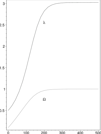
Figure 1: Numerical flow for $\lambda$ and $\Omega$

Of course to establish fully rigorously this picture is beyond the reach of perturbative theorems and requires a constructive analysis.

III Multi-Scale analysis and the Beta function

The best perturbative expansion is neither the bare expansion, which has no subtractions, hence no ultraviolet limit, nor the renormalized expansion, which has too many, but the effective expansion, which has just the necessary ones [13]. Accordingly the best scheme to compute the evolution of the effective coupling, hence the beta function, is also the effective expansion, and it is the one used in this paper. The effective expansion requires some kind of multiscale analysis. Since at $\Omega=1$ the theory is an exact matrix theory, that is integers are conserved along the ribbon sides, hence the faces, it is convenient to define this multiscale analysis at the level of the variables associated to each face rather than at the propagator level.

III.1 Cutoff, Slices

Every ribbon graph in this theory has $n$ vertices, $L$ internal lines, $N$ external legs, $F$ faces, a genus $g$ such that $2-2g=n-L+F$ and a number $B$ of broken or ”external” faces. Only graphs with $g=0$, $B=1$ and $N\leq 4$ are divergent and enter the RG flow equations.

Putting separately the cutoff on the face variables means that the theory with ultraviolet cutoff $M^{\rho}$ and infrared cutoff $M^{i}$, $i<\rho$, is the sum over all graphs which have all the integers $m$ associated to their $F-B$ unbroken ”internal” faces between $M^{i}$ and $M^{\rho}$: $M^{i}\leq m\leq M^{\rho}$. Here $m$ means $m_{1}+m_{2}$ because Moyal ${\mathbb{R}}^{4}$ is made of two symplectic pairs, hence every face variable is in fact made of two integers $m_{1}$ and $m_{2}$.

The part of the theory in the $i$-th slice is the difference between the theory with infrared cutoff respectively $M^{i+1}$ and $M^{i}$ so it is the sum over all graphs which have all the integers associated to their $F-B$ unbroken ”internal” faces between $M^{i}$ and $M^{\rho}$, at least one of them being exactly between $M^{i}$ and $M^{i+1}$.

As well known the effective expansion has only ”useful” renormalization performed. As a consequence it is an expansion in terms of effective couplings. ”Useful” renormalization means (in our context of cutoffs on faces) that we subtract only divergent subgraphs with all their internal face variables in higher slices than all their external variables.

III.2 The effective theory

Now how does one compute the beta function, namely the flow for the effective vertex of the theory?

Mass Renormalization

To simplify further the effective expansion rules let us remark that the mass renormalization is somewhat special since it is the only non-logarithmic. In any $\phi^{4}$ theory it is easy to check that 1PI subgraphs never overlap. Therefore it is not necessary to use RG to disentangle ”overlapping” mass divergences. Instead of using effective masses and useful mass subtractions, it is therefore convenient to treat the renormalization of mass in the good old pre-Wilsonian way, namely to use the renormalized mass $\mu$ in the propagator and to mass-renormalize the perturbation expansion independent of scale attributions (see [13], end of Chapter II.4). Of course this does not work for the coupling constant because there are ”overlapping” four point divergences, and RG is truly necessary to disentangle them.

So we adopt the rule that in any Feynman graph of the theory any one particle irreducible two point subgraph is always subtracted by the corresponding mass counterterm, and the subtraction is performed irrespective of the internal and external scales.

Effective Vertices

Once mass renormalizations have been taken care of, there remains three kinds of log divergent subtractions: the four point functions, whose counterterms are of the $\phi^{*4}$ form like the initial Lagrangian interaction, and the two ”two point function second subtractions” which correspond to the $p^{2}\phi^{2}$ and $\tilde{x}^{2}\phi^{2}$ terms of the initial Lagrangian.

If we were to perform the useful subtractions for all these three operators, we would end up with an effective theory with effective couplings and effective propagators. But effective propagators are very inconvenient to use (since they are already used for the slicing itself…). It is more convenient to remark that at $\Omega=1$ the $p^{2}\phi^{2}$ and $\tilde{x}^{2}\phi^{2}$ terms follow exactly the same RG trajectory so that their effective coefficients remain equal, at any order ([1], last section). It corresponds indeed in the language of [1] to the vanishing of the $\Omega$ flow at all loops at $\Omega=1$, which is a simple and direct consequence of the exact matrix character of the theory at $\Omega=1$. As a consequence we can absorb the effective coefficients $p^{2}$ and $\tilde{x}^{2}$ terms of the initial Lagrangian into a single ”field strength renormalization” which is $Z^{1/2}$, where $Z$ is the propagator renormalization. In this way we keep the propagator coefficients fixed over all slices. In other words, and since there are 4 fields per vertex, we can over all RG slices use the same fixed propagator (II.1), provided we do not use as effective coupling $\Gamma^{4}$ but the effective vertex $\lambda_{i}=[\Gamma^{4}/Z^{2}]_{i}$.

Now to compute the beta function we have to compute the change in this effective vertex when one RG slice $i$ is added in the infrared direction, and the ultra violet limit $\rho\to\infty$ is performed. This change $\lambda_{i}-\lambda_{i+1}$ is therefore the sum over all contributions to this effective vertex $\Gamma^{4}/Z^{2}$ which have:

• all their internal faces in slices $j\geq i$, with at least one exactly in the slice $i$,

• their (single) external face index taken at the renormalization point, that is at 0 for the 4 point graphs of $\Gamma^{4}$ and at first derivative at 0 for the 2 point graphs of $Z$, see below,

• their mass subtractions performed for all their 1PI two point subgraphs,

• their useful 4 and 2 point log divergent subtractions performed, that is for all their 2 and 4 point subgraphs whose internal scales are all strictly bigger than their external scales.

• an effective coupling $\lambda_{j}$ at each vertex whose maximal index is $j$.

The vanishing of the beta function (in the UV regime) means that the change $\delta\lambda_{i}=\lambda_{i}-\lambda_{i+1}$ tends to 0 as $i\to\infty$, and the boundedness of the RG flow is the slightly stronger assumption that this change not only tends to zero but is summable over $i$. Remark that the total flow $\lambda_{ren}-\lambda_{bare}$ (where $\lambda_{ren}=\lambda_{0}$ and $\lambda_{bare}=\lim_{\rho\to\infty}\lambda_{\rho}$) in general is never zero, because $\delta\lambda_{i}$ is not exactly zero, in particular for the first values of $i$. The difference between the bare and effective vertices is really expressed by the finite $\gamma$ series in (II.11).

If the constructive version of this theory can ever be built as we expect, this $\gamma$ series will hopefully be shown Borel summable and its Borel sum should be the non-perturbative finite flow between the bare and the renormalized coupling.

If we inductively know that the beta function vanishes up to order $p$ and study its vanishing at order $p+1$, then we know that the difference between any effective coupling $\lambda_{j}$ and the effective coupling $\lambda_{i}$ tends uniformly to zero as $i\to\infty$, so that we can completely forget point e) above and replace all $p+1$ effective vertices $\lambda_{j}$ by a same coupling, eg $\lambda_{i}$ or $\lambda_{bare}$ itself, since the difference will be higher order times finite coefficients. This is what we do below: we always multiply each contribution of order $p$ by $\lambda^{p}$ where $\lambda$ is the bare coupling.

Further simplifications are also used below to minimize the amount of actual computations. In the main identity (II.11), many graphs cancel out completely at the ”bare level”. Computing their mass renormalized amplitudes and the useful renormalizations for coupling constant and wave function counterterms would be completely fastidious because these renormalized values always also cancel out if the bare values do! So to simplify the computation we list first all the main bare (unrenormalized) divergent sums for all possible graphs up to three loops. These graphs must be planar, which helps make them tractable with some care. Then we work out all combinatoric factors and cancel out many bare sums. Only for the remaining terms (which do not cancel out) do we need to apply the mass subtractions and the eventual useful log divergent subtractions.

Up to three loops it happens that only tadpoles mass subtractions are in fact necessary, because bare amplitudes with mass ”sunshines” insertions such as those of graphs $CS$ and $BS$ cancel out completely in (II.11). It happens also that only useful wave-function subtractions of tadpoles are necessary. Of course we suspect that tadpole subtractions only will not be enough at more than 3 loops.

IV Basic Sums

We introduce now systematic notations for the basic integers sums which are the amplitudes of the two point or four-point Feynman graphs in this theory. These sums without further limitations are divergent, but as explained in the previous section we will in fact always compute them with one index (at least) in the $i$-th slice, the others above. Subtractions for the mass divergences and for the ”useful” subtractions for the log divergences are always performed even if not explicitly indicated, so that the real sums which we manipulate are always finite.

This being recalled, the structure of the sums up to three loops are performed over at most three face integers denoted as $p,q,r$. They have to be symmetric because our cutoffs only depend on these face indices (not on the propagators which depend on the sum of two integers on adjacent faces).

The upper index in our basic sums is (1), (2) or (3) and recalls the perturbation order. At order 1 there is only one graph B1 (see Figure 5). The corresponding sum is:

$${\cal S}^{(1)}_{1}=\sum_{p}\tfrac{1}{(A+p)^{2}}\qquad(B1)\ .$$ (IV.1)

At order two there are 4 graphs (see Figure 5 again):

$${\cal S}^{(2)}_{1} =[{\cal S}_{1}^{(1)}]^{2}=\sum_{p,q}\tfrac{1}{(A+p)^{2}}\tfrac{1}{(A+q)^{2}}\quad(B2)\ ,\quad {\cal S}^{(2)}_{3} =\sum_{p,q}\tfrac{1}{(A+p)^{3}}\tfrac{1}{(A+q)}\quad\ \ (TEXT)\ ,$$

$${\cal S}^{(2)}_{2} =\sum_{p,q}\tfrac{1}{(A+p)^{2}}\tfrac{1}{(A+p+q)}\tfrac{1}{(A+q)}\quad\ \ \ (E)\ ,\quad {\cal S}^{(2)}_{4} =\sum_{p,q}\tfrac{1}{(A+p)^{3}}\tfrac{1}{(A+p+q)}\ \ (TINT)\ .$$ (IV.2)

At order three there are more graphs (see Figures 6,7):

$${\cal S}^{(3)}_{1} =\sum_{p,q,r}\tfrac{1}{(A+p)^{2}(A+q)^{2}(A+r)^{2}}=(\Sigma_{1}^{1})^{3}\quad (B3)$$ (IV.3)

$${\cal S}^{(3)}_{2} =\sum_{p,q,r}\tfrac{1}{(A+p)^{2}(A+q)(A+r)(A+p+q)(A+q+r)}\quad (TrE)$$ (IV.4)

$${\cal S}^{(3)}_{3} =\sum_{p,q,r}\tfrac{1}{(A+p)^{2}(A+q)(A+r)(A+p+q)(A+p+r)}\quad (EYB2,\ BEB)$$ (IV.5)

$${\cal S}^{(3)}_{4} =\sum_{p,q,r}\tfrac{1}{(A+p)^{2}(A+q)^{2}(A+r)(A+q+r)}\quad (BEY)$$ (IV.6)

$${\cal S}^{(3)}_{5} =\sum_{p,q,r}\tfrac{1}{(A+p)^{2}(A+q)^{2}(A+p+r)(A+q+r)}\quad (EY2)$$ (IV.7)

$${\cal S}^{(3)}_{6} =\sum_{p,q,r}\tfrac{1}{(A+p)^{2}(A+q)^{2}(A+p+q)(A+q+r)}\quad (ETSI)$$ (IV.8)

$${\cal S}^{(3)}_{7} =\sum_{p,q,r}\tfrac{1}{(A+p)^{2}(A+q)(A+p+q)^{2}(A+q+r)}\quad (EITD)$$ (IV.9)

$${\cal S}^{(3)}_{8} =\sum_{p,q,r}\tfrac{1}{(A+p)^{2}(A+q)(A+p+q)^{2}(A+p+r)}\quad (EITG)$$ (IV.10)

$${\cal S}^{(3)}_{9} =\sum_{p,q,r}\tfrac{1}{(A+p)^{2}(A+q)^{2}(A+r)(A+p+q)}\quad (ETSE)$$ (IV.11)

$${\cal S}^{(3)}_{10} =\sum_{p,q,r}\tfrac{1}{(A+p)^{3}(A+q)(A+p+q)(A+p+r)}\quad (ETI)$$ (IV.12)

$${\cal S}^{(3)}_{11} =\sum_{p,q,r}\tfrac{1}{(A+p)^{3}(A+q)(A+r)(A+p+q)}\quad (ETE)$$ (IV.13)

$${\cal S}^{(3)}_{12} =\sum_{p,q,r}\tfrac{1}{(A+p)^{3}(A+q)^{2}(A+p+r)}\quad (B2TI)$$ (IV.14)

$${\cal S}^{(3)}_{13} =\sum_{p,q,r}\tfrac{1}{(A+p)^{3}(A+q)^{2}(A+r)}\quad (B2TE,\ BT2EE)$$ (IV.15)

$${\cal S}^{(3)}_{14} =\sum_{p,q,r}\tfrac{1}{(A+p)^{3}(A+q)(A+p+r)(A+q+r)}\quad (BS)$$ (IV.16)

$${\cal S}^{(3)}_{15} =\sum_{p,q,r}\tfrac{1}{(A+p)^{3}(A+p+q)^{2}(A+q+r)}\quad (BT2II)$$ (IV.17)

$${\cal S}^{(3)}_{16} =\sum_{p,q,r}\tfrac{1}{(A+p)^{3}(A+p+q)^{2}(A+p+r)}\quad (BT2IE)$$ (IV.18)

$${\cal S}^{(3)}_{17} =\sum_{p,q,r}\tfrac{1}{(A+p)^{3}(A+q)^{2}(A+q+r)}\quad (BT2EIE)$$ (IV.19)

$${\cal S}^{(3)}_{18} =\sum_{p,q,r}\tfrac{1}{(A+p)^{4}(A+q)(A+p+r)}\quad (BEI,\ BIE,\ EBI)$$ (IV.20)

$${\cal S}^{(3)}_{19} =\sum_{p,q,r}\tfrac{1}{(A+p)^{4}(A+p+q)(A+p+r)}\quad (BII,\ IBI)$$ (IV.21)

$${\cal S}^{(3)}_{20} =\sum_{p,q,r}\tfrac{1}{(A+p)^{4}(A+q)(A+r)}\quad (BEE,\ EBE)$$ (IV.22)

where the names refer to the graphs pictured on the corresponding figures. We study first $Z$, which involves a smaller number of graphs, and then $\Gamma_{4}$.

V Study of $Z$

Lemma 1

For $\phi^{4}_{4}$ and $(\bar{\Phi}\Phi)^{2}$ we have at three loops

$$Z=1-a\tilde{\lambda}+b\tilde{\lambda}^{2}-c\tilde{\lambda}^{3}$$ (V.1)

where $\tilde{\lambda}=\tfrac{\lambda}{(4\pi)^{2}}$ and both in the real and complex case

$$a = \frac{1}{4}{\cal S}_{1}^{(1)}$$ (V.2)

$$b = \frac{1}{16}[{\cal S}^{(2)}_{1}+{\cal S}^{(2)}_{2}+2({\cal S}^{(2)}_{3}+{\cal S}^{(2)}_{4})]$$ (V.3)

$$c = \frac{1}{4^{3}}\bigg{[}({\cal S}_{1}^{(3)}+{\cal S}_{3}^{(3)}+{\cal S}_{4}^{(3)}+{\cal S}_{5}^{(3)}+{\cal S}_{6}^{(3)}+{\cal S}_{7}^{(3)}+{\cal S}_{8}^{(3)}+{\cal S}_{9}^{(3)})$$ (V.4)

$$+2\big{(}{\cal S}_{2}^{(3)}+{\cal S}_{10}^{(3)}+{\cal S}_{11}^{(3)}+{\cal S}_{14}^{(3)}+{\cal S}_{15}^{(3)}+{\cal S}_{16}^{(3)}+{\cal S}_{17}^{(3)}\big{)}$$

$$+3({\cal S}_{19}^{(3)}+{\cal S}_{20}^{(3)})+4{\cal S}_{12}^{(3)}+6({\cal S}_{13}^{(3)}+{\cal S}_{18}^{(3)})\bigg{]}\ .$$

The rest of the section is devoted to the proof.

V.1 The Self-Energy

Lemma 2

The self-energy up to order three, after taking away the factor $(4\pi)^{2}\theta$, is

$$\tfrac{1}{(4\pi)^{2}\theta}\Sigma_{m,n}=-\tilde{\lambda}A_{mn}+\tilde{\lambda}^{2}B_{mn}-\tilde{\lambda}^{3}C_{mn}$$ (V.5)

where

$$A_{mn} =\frac{1}{4}\sum_{p}[\underbrace{\tfrac{1}{A+p+m}}_{Tup}+\underbrace{m\leftrightarrow n}_{Tdown}]$$ (V.6)

$$B_{mn} =\frac{1}{4^{2}}\sum_{p,q}[\underbrace{\tfrac{1}{(A+p+m)(A+q+n)(A+p+q)}}_{S}+\underbrace{(\tfrac{1}{(A+p+m)^{2}(A+q+m)}}_{TEXTup}$$

$$\qquad\qquad\quad+\underbrace{\tfrac{1}{(A+p+m)^{2}(A+p+q)}}_{TINTup}+m\leftrightarrow n)]$$

$$C_{mn} =\frac{1}{4^{3}}\sum_{p,q,r}[\underbrace{\tfrac{1}{(A+p+m)(A+q+n)(A+r+n)(A+p+q)(A+p+r)}}_{TB2}+$$

$$+\underbrace{\tfrac{1}{(A+p+n)^{2}(A+q+n)(A+q+r)(A+p+r)}}_{CS}+\underbrace{\tfrac{1}{(A+q+m)(A+p+n)^{2}(A+p+q)(A+r+n)}}_{STE}+$$

$$+\underbrace{\tfrac{1}{(A+q+m)(A+p+n)^{2}(A+p+q)(A+p+r)}}_{STI}+\underbrace{\tfrac{1}{(A+q+m)(A+p+n)(A+p+q)^{2}(A+p+r)}}_{STS}+$$

$$+\underbrace{\tfrac{1}{(A+p+n)^{2}(A+p+q)^{2}(A+q+r)}}_{CITI}+\underbrace{\tfrac{1}{(A+p+n)^{2}(A+p+q)^{2}(A+p+r)}}_{CITE}+\underbrace{\tfrac{1}{(A+p+n)^{2}(A+q+n)^{2}(A+q+r)}}_{CETI}+$$

$$+\underbrace{\tfrac{1}{(A+p+n)^{2}(A+q+n)^{2}(A+r+n)}}_{CETE}+\underbrace{\tfrac{1}{(A+p+n)^{3}(A+p+q)(A+p+r)}}_{CII}+\underbrace{\tfrac{2}{(A+p+n)^{3}(A+q+n)(A+p+r)}}_{CIEL\ +\ CIER}+$$

$$+\underbrace{\tfrac{1}{(A+p+n)^{3}(A+q+n)(A+r+n)}}_{CEE}+m\leftrightarrow n]$$ (V.7)

and the corresponding graphs are listed in Figures 2,3 and 4.

Figure 2: Two Point Graphs at one Loops: the up and down tadpoles

Proof

At one loop we have only one vertex and one line, therefore, after taking out the factor $(4\pi)^{2}\theta$ we have

$$-\tilde{\lambda}(4\pi^{2}\theta^{2})(4\pi)^{2}\tfrac{1}{[(4\pi)^{2}\theta]^{2}}\sum_{G}\tfrac{K_{G}}{4}(S_{G}^{(1)})_{mn}=-\frac{\tilde{\lambda}}{4}\sum_{G}\tfrac{K_{G}}{4}(S_{G}^{(1)})_{mn}$$ (V.8)

where $G$ are the graphs at one loop (there are two of them, see Figure 2), $(S_{G}^{(1)})_{mn}$ are the corresponding amplitudes (listed above) and $K_{G}$ is a combinatorial factor. The combinatorial factors for $T\ up$ and $T\ down$ are the same

$$K_{G}^{r}=4\ \Rightarrow\frac{K^{r}_{G}}{4}=1\ .$$ (V.9)

In the complex case we have instead of $K_{G}^{r}/4$ the term $K_{G}^{c}/2$ and $K_{G}^{c}=2$. So in both cases we have

$$A_{mn}=\frac{1}{4}\sum_{G}(S_{G}^{(1)})_{mn}\ .$$ (V.10)

At two loops we have two vertices and three lines, therefore, after taking out the factor $(4\pi)^{2}\theta$ we have

$$\tfrac{1}{2!}\tilde{\lambda}^{2}(4\pi^{2}\theta^{2})^{2}(4\pi)^{4}\tfrac{1}{[(4\pi)^{2}\theta]^{4}}\sum_{G}\tfrac{K_{G}}{4^{2}}(S_{G}^{(2)})_{mn}=\tfrac{\tilde{\lambda}^{2}}{4^{2}}\tfrac{1}{2}\sum_{G}\tfrac{K_{G}}{4^{2}}(S_{G}^{(2)})_{mn}$$ (V.11)

where $G$ are the graphs at two loops of Figure 3, $(S_{G}^{(2)})_{mn}$ are the corresponding amplitudes (listed above) and $K_{G}$ is again a combinatorial factor. As before, in the complex case instead of $K_{G}^{r}/4$ we have $K_{G}^{c}/2$. The factors (in the real case) are

$$K_{S}^{r}=2\cdot 4^{2}\ ,\quad K_{T2EXTup}^{r}=2\cdot 4^{2}\ ,\quad K_{T2INTup}^{r}=2\cdot 4^{2}\ .$$ (V.12)

The same factors hold for the graphs with $m$ and $n$ exchanged. In the complex case we have

$$K_{S}^{r}=2\cdot 2^{2}\ ,\quad K_{T2EXTup}^{r}=2\cdot 2^{2}\ ,\quad K_{T2INTup}^{r}=2\cdot 2^{2}\ .$$ (V.13)

so in both cases we have

$$B_{mn}=\frac{1}{4^{2}}\sum_{G}(S_{G})^{(2)}_{mn}\ .$$ (V.14)

Figure 3: Two Point Graphs at Two Loops

At three loops we have three vertices and five lines, therefore, after taking out the factor $(4\pi)^{2}\theta$ we have

$$-\frac{1}{3!}\tilde{\lambda}^{3}(4\pi^{2}\theta^{2})^{3}(4\pi)^{6}\frac{1}{[(4\pi)^{2}\theta]^{6}}\sum_{G}\frac{K_{G}}{4^{3}}(S_{G}^{(3)})_{mn}=-\frac{\tilde{\lambda}^{3}}{4^{3}}\frac{1}{3!}\sum_{G}\frac{K_{G}}{4^{3}}(S_{G}^{(3)})_{mn}$$ (V.15)

where $G$ are the graphs at three loops (Figure 4), $(S_{G}^{(3)})_{mn}$ are the corresponding amplitudes (listed above) and $K_{G}$ is again a combinatorial factor. As before, in the complex case instead of $K_{G}^{r}/4$ we have $K_{G}^{c}/2$. The factors (in the real case and complex case) are

$$K_{G}^{r}=3!\ 4^{3}\ ,\qquad K_{G}^{r}=3!\ 2^{3}\qquad\forall G\ ,$$ (V.16)

therefore in both cases

$$C_{mn}=\tfrac{1}{4^{3}}\sum_{G}(S_{G})^{(3)}_{mn}\ .$$ (V.17)

This completes the proof of the lemma.

Figure 4: Two Point Graphs at Three Loops

V.2 Proof of lemma 1

Now from the definition of $Z$, to prove lemma 1 we need to compute

$$a= -\left.\partial_{m_{1}}A_{mn}\right|_{m=n=0}=-\left.\partial_{n_{1}}A_{mn}\right|_{m=n=0}\ ,$$

$$b= -\left.\partial_{m_{1}}B_{mn}\right|_{m=n=0}=-\left.\partial_{n_{1}}B_{mn}\right|_{m=n=0}\ ,$$

$$c= -\left.\partial_{m_{1}}C_{mn}\right|_{m=n=0}=-\left.\partial_{n_{1}}C_{mn}\right|_{m=n=0}\ .$$ (V.18)

From the definitions of $A_{mn}$, $B_{mn}$ and $C_{mn}$ we get

$$a=\frac{1}{4}\sum_{p}[\underbrace{\tfrac{1}{(A+p)^{2}}}_{Tup}+\underbrace{0}_{Tdown}]\ =\ \tfrac{1}{4}{\cal S}_{1}^{(1)}\ .$$ (V.19)

$$b= \frac{1}{4^{2}}\sum_{p,q,r}[\underbrace{\tfrac{1}{(A+p)^{2}(A+q)(A+p+q)}}_{S}+\underbrace{\left(2\tfrac{1}{(A+p)^{3}(A+q)}+\tfrac{1}{(A+p)^{2}(A+q)^{2}}\right)}_{TEXTup}+\underbrace{2\tfrac{1}{(A+p)^{3}(A+p+q)}}_{TINTup}+0)]$$

$$= \frac{1}{16}[{\cal S}^{(2)}_{1}+{\cal S}^{(2)}_{2}+2({\cal S}^{(2)}_{3}+{\cal S}^{(2)}_{4})]\ .$$ (V.20)

$$c =\frac{1}{4^{3}}\sum_{p,q,r}\bigg{[}\underbrace{{\cal S}_{3}^{(3)}+2{\cal S}_{2}^{(3)}}_{TB2+m\leftrightarrow n}+\underbrace{2{\cal S}_{14}^{(3)}+{\cal S}_{5}^{(3)}}_{CS+m\leftrightarrow n}+\underbrace{{\cal S}_{9}^{(3)}+2{\cal S}_{11}^{(3)}+{\cal S}_{4}^{(3)}}_{STE+m\leftrightarrow n}+$$

$$+\underbrace{{\cal S}_{6}^{(3)}+2{\cal S}_{10}^{(3)}}_{STI+m\leftrightarrow n}+\underbrace{{\cal S}_{8}^{(3)}+{\cal S}_{7}^{(3)}}_{STS+m\leftrightarrow n}+\underbrace{2{\cal S}_{15}^{(3)}}_{CITI+m\leftrightarrow n}+\underbrace{2{\cal S}_{16}^{(3)}}_{CITE+m\leftrightarrow n}+\underbrace{2{\cal S}_{17}^{(3)}+2{\cal S}_{12}^{(3)}}_{CETI+m\leftrightarrow n}+$$

$$+\underbrace{4{\cal S}_{13}^{(3)}+{\cal S}_{1}^{(3)}}_{CETE+m\leftrightarrow n}+\underbrace{3{\cal S}_{19}^{(3)}}_{CII+m\leftrightarrow n}+\underbrace{2(3{\cal S}_{18}^{(3)}+{\cal S}_{12}^{(3)})}_{CIEL\ +\ CIER+m\leftrightarrow n}+\underbrace{3{\cal S}_{20}^{(3)}+2{\cal S}_{13}^{(3)}}_{CEE+m\leftrightarrow n}\bigg{]}\ ,$$ (V.21)

so that putting these together

$$c =\frac{1}{4^{3}}\big{[}({\cal S}^{(3)}_{1}+{\cal S}^{(3)}_{3}+{\cal S}^{(3)}_{4}+{\cal S}^{(3)}_{5}+{\cal S}^{(3)}_{6}+{\cal S}^{(3)}_{7}+{\cal S}^{(3)}_{8}+{\cal S}^{(3)}_{9})+2({\cal S}^{(3)}_{2}+{\cal S}^{(3)}_{10}$$

$$+{\cal S}^{(3)}_{11}+{\cal S}^{(3)}_{14}+{\cal S}^{(3)}_{15}+{\cal S}^{(3)}_{16}+{\cal S}^{(3)}_{17})+3({\cal S}^{(3)}_{19}+{\cal S}^{(3)}_{20})+4{\cal S}^{(3)}_{12}+6({\cal S}^{(3)}_{13}+{\cal S}^{(3)}_{18})\big{]}\ .$$ (V.22)

VI Study of $\Gamma_{4}$

Lemma 3

For both $\phi^{4}_{4}$ and $(\bar{\Phi}\Phi)^{2}$ we have at three loops, before performing the mass renormalization

$$\Gamma_{4}(0,0,0,0)=-\lambda(4\pi^{2}\theta^{2})[1-a^{\prime}\tilde{\lambda}+b^{\prime}\tilde{\lambda}^{2}-c^{\prime}\tilde{\lambda}^{3}]$$ (VI.1)

where $\tilde{\lambda}=\tfrac{\lambda}{(4\pi)^{2}}$ and

$$a^{\prime} = \frac{1}{2}{\cal S}_{1}^{(1)}$$ (VI.2)

$$b^{\prime} = \frac{1}{8}[{\cal S}^{(2)}_{1}+2({\cal S}^{(2)}_{2}+{\cal S}^{(2)}_{3}+{\cal S}^{(2)}_{4})]$$ (VI.3)

$$c^{\prime} = \frac{1}{32}\bigg{[}({\cal S}^{(3)}_{1}+{\cal S}^{(3)}_{5})+2({\cal S}^{(3)}_{4}+{\cal S}^{(3)}_{6}+{\cal S}^{(3)}_{7}+{\cal S}^{(3)}_{8}+{\cal S}^{(3)}_{9}$$ (VI.4)

$$\quad\ +{\cal S}^{(3)}_{14}+{\cal S}^{(3)}_{15}+{\cal S}^{(3)}_{16}+{\cal S}^{(3)}_{17})+3({\cal S}^{(3)}_{3}+{\cal S}^{(3)}_{19}+{\cal S}^{(3)}_{20})$$

$$\quad\ +4({\cal S}^{(3)}_{4}+{\cal S}^{(3)}_{10}+{\cal S}^{(3)}_{11}+{\cal S}^{(3)}_{12})+6({\cal S}^{(3)}_{13}+{\cal S}^{(3)}_{18})\bigg{]}$$

and the corresponding graphs are drawn in Figure 5, 6 and 7.

The rest of this section is devoted to the proof.

VI.1 One Loop

At one loop there is only one graph contributing to $\Gamma_{4}$, the bubble $B1$ in Figure 5.

Figure 5: Four Point Graphs at one and two Loops

This graph has two vertices and two lines, plus a factor $1/2!$ from the exponential. After taking out the factors $-\lambda(4\pi^{2}\theta^{2}(-\tilde{\lambda})$ we have, in the real case

$$a^{\prime}\ =\ \frac{1}{8}\left(\frac{K_{r}(B)}{4^{2}}\right)\sum_{p\in\mathbb{N}^{2}}\tfrac{1}{(A+p)^{2}}\ =\ \frac{1}{8}\left(\frac{K_{r}(B)}{4^{2}}\right){\cal S}_{1}^{(1)}\ ,$$ (VI.5)

where $K_{r}(B)=4^{3}$ is the combinatoric factor counting the number of times this graph appears. In the complex case we get the same expression, except that instead of $K_{r}(B)/4^{2}$ we have $K_{c}(B)/2^{2}$ and the combinatoric factor is now $K_{c}(B)=2^{4}$.

$$\frac{K_{r}(B)}{4^{2}}=\frac{K_{c}(B)}{2^{2}}=4\ .$$ (VI.6)

The result is

$$a^{\prime}=\frac{1}{2}\sum_{p}\tfrac{1}{(A+p)^{2}}=\frac{1}{2}{\cal S}^{(1)}_{1}=2a\ .$$ (VI.7)

VI.2 Two Loops

At two loops there are four graphs $B2$ (double bubble), $E$ (eye), $BEXT$, $BINT$ (see Figure 5). So in the real case

$$b^{\prime}=\frac{1}{3!\ 4^{2}}\sum_{G}\frac{K_{r}(G)}{4^{3}}S_{G}(p,q)\ ,$$ (VI.8)

where

$$S_{B2}=\sum_{p,q}\tfrac{1}{(A+p)^{2}}\tfrac{1}{(A+q)^{2}}=\Sigma^{2}_{1}=({\cal S}_{1}^{(1)})^{2}\ , S_{E}=\sum_{p,q}\tfrac{1}{(A+p)^{2}}\tfrac{1}{A+q}\tfrac{1}{(A+p+q)}={\cal S}^{(2)}_{2}\ ,$$

$$S_{BEXT}=\sum_{p,q}\tfrac{1}{(A+p)^{3}}\tfrac{1}{A+q}={\cal S}^{(2)}_{3}\ , S_{BINT}=\sum_{p,q}\tfrac{1}{(A+p)^{3}}\tfrac{1}{A+p+q}={\cal S}^{(2)}_{4}\ .$$ (VI.9)

In the complex case we have the same expression with $K_{c}(G)/2^{3}$ instead of $K_{r}(G)/4^{3}$. The combinatorial coefficients in the real case are

$$K_{r}(E)=K_{r}(BEXT)=K_{r}(BINT)=3!\cdot 4^{3}\cdot 4\ ,\qquad K_{r}(B2)=3!\cdot 4^{3}\cdot 2\ ,$$ (VI.10)

and in the complex one are

$$K_{c}(E)=K_{c}(BEXT)=K_{c}(BINT)=3!\cdot 2^{3}\cdot 4\ ,\qquad K_{c}(B2)=3!\cdot 2^{3}\cdot 2\ ,$$ (VI.11)

so

$$\tfrac{K_{r}(E)}{4^{3}}=\tfrac{K_{c}(E)}{2^{3}}=\tfrac{K_{r}(BEXT)}{4^{3}}=\tfrac{K_{c}(BEXT)}{2^{3}}=\tfrac{K_{r}(BINT)}{4^{3}}=\tfrac{K_{c}(BINT)}{2^{3}}=3!\cdot 4\ ,$$

$$\tfrac{K_{r}(B2)}{4^{3}}=\tfrac{K_{c}(B2)}{2^{3}}=3!\cdot 2\ .$$ (VI.12)

and

$$b^{\prime}=\frac{1}{8}[{\cal S}^{(2)}_{1}+2({\cal S}^{(2)}_{2}+{\cal S}^{(2)}_{3}+{\cal S}^{(2)}_{4})]\ .$$ (VI.13)

VI.3 Three Loops

At three loops the 26 graphs contributing to $\Gamma_{4}$ are drawn with their code names in Figures 6 and 7 .

Figure 6: Four Point Graphs at Three Loops, Part I

After eliminating $-\lambda 4\pi^{2}\theta^{2}$ from $(-\lambda 4\pi^{2}\theta^{2})^{4}\tfrac{1}{4!}\tfrac{1}{[(4\pi)^{2})\theta]^{6}}\tfrac{1}{4^{4}}$ and a $-(\tilde{\lambda})^{3}$ the value of $c^{\prime}$ is

$$c^{\prime}=\frac{1}{4!}\frac{1}{4^{3}}\sum_{i=1}^{20}\frac{K_{i}}{4^{4}}{\cal S}^{(3)}_{i}\ .$$ (VI.14)

Figure 7: Four Point Graphs at Three Loops, Part II

For the real case we have

$$K_{1} =4!4^{4}\cdot 2\qquad(B3) K_{2} =4!4^{4}\cdot 4\cdot 2\quad(TrE)$$ (VI.15)

$$K_{3} =4!4^{4}\cdot 6\qquad(4EYB2+2BEB) K_{4} =4!4^{4}\cdot 4\qquad(BEY)$$

$$K_{5} =4!4^{4}\cdot 2\qquad(EY2) K_{6} =4!4^{4}\cdot 4\qquad(ETSI)$$

$$K_{7} =4!4^{4}\cdot 4\qquad(EITD) K_{8} =4!4^{4}\cdot 4\qquad(EITG)$$

$$K_{9} =4!4^{4}\cdot 4\qquad(ETSE) K_{10} =4!4^{4}\cdot 8\qquad(ETI)$$

$$K_{11} =4!4^{4}\cdot 8\qquad(ETE) K_{12} =4!4^{4}\cdot 8\qquad(B2TI)$$

$$K_{13} =4!4^{4}\cdot 12\quad\ (B2TE+BT2E) K_{14} =4!4^{4}\cdot 4\qquad(BS)$$

$$K_{15} =4!4^{4}\cdot 4\qquad(BT2II) K_{16} =4!4^{4}\cdot 4\qquad(BT2IE)$$

$$K_{17} =4!4^{4}\cdot 4\qquad(BT2EI) K_{18} =4!4^{4}\cdot 12\quad\ (BEI+BIE+EBI)$$

$$K_{19} =4!4^{4}\cdot 6\qquad(BII+IBI) K_{20} =4!4^{4}\cdot 6\qquad(BEE+EBE)$$

In the complex case the coefficients are the same, except the $4^{4}$ factor becomes a $2^{4}$ one (at each vertex we have two choices instead of four to contract a particular field), so both in the real and complex case we have

$$c^{\prime} =\frac{1}{32}[({\cal S}^{(3)}_{1}+{\cal S}^{(3)}_{5})+2({\cal S}^{(3)}_{4}+{\cal S}^{(3)}_{6}+{\cal S}^{(3)}_{7}+{\cal S}^{(3)}_{8}+{\cal S}^{(3)}_{9}+{\cal S}^{(3)}_{14}+{\cal S}^{(3)}_{15}+{\cal S}^{(3)}_{16}+{\cal S}^{(3)}_{17})$$

$$+3({\cal S}^{(3)}_{3}+{\cal S}^{(3)}_{19}+{\cal S}^{(3)}_{20})+4({\cal S}^{(3)}_{2}+{\cal S}^{(3)}_{10}+{\cal S}^{(3)}_{11}+{\cal S}^{(3)}_{12})+6({\cal S}^{(3)}_{13}+{\cal S}^{(3)}_{18})].$$ (VI.16)

VII Beta function and Proof of the Theorem

For the beta function the important combination is

$$-\frac{1}{\lambda(4\pi^{2}\theta^{2})}\frac{\Gamma_{4}}{Z^{2}} = \frac{1-a^{\prime}\tilde{\lambda}+b^{\prime}\tilde{\lambda}^{2}-c^{\prime}\tilde{\lambda}^{3}}{[1-a\tilde{\lambda}+b\tilde{\lambda}^{2}-c\tilde{\lambda}^{3}]^{2}}$$

$$= [1-\gamma_{1}\tilde{\lambda}+\gamma_{2}\tilde{\lambda}^{2}-\gamma_{3}\tilde{\lambda}^{3}+O(\lambda^{4})]$$

and we need to prove that each $\gamma$ is finite. In fact it turns out that since $a^{\prime}=2a$, $\gamma_{1}=0$ so multiplying by $Z^{2}$ and expanding out, the equations to prove are:

$$a^{\prime}=2a\ ;\ b^{\prime}=2b+a^{2}+\gamma_{2}\ ;\ c^{\prime}=2c+2ab+2a\gamma_{2}+\gamma_{3}\ .$$ (VII.2)

VII.1 One and Two loops

Let us prove the two first equations. For $\Omega=1$, $a=a^{\prime}/2$, hence the first equation $a^{\prime}=2a$ holds and

$$b^{\prime}-2b+3a^{2}-2aa^{\prime} = b^{\prime}-2b-\tfrac{1}{4}{a^{\prime}}^{2}=\tfrac{1}{8}[{\cal S}^{(2)}_{1}+2({\cal S}^{(2)}_{2}+{\cal S}^{(2)}_{3}+{\cal S}^{(2)}_{4})]$$ (VII.3)

$$-\frac{1}{8}[{\cal S}^{(2)}_{1}+{\cal S}^{(2)}_{2}+2({\cal S}^{(2)}_{3}+{\cal S}^{(2)}_{4})]-\frac{1}{16}({\cal S}_{1}^{(1)})^{2}\$$

$$= \ \frac{1}{16}[2{\cal S}^{(2)}_{2}-{\cal S}^{(2)}_{1}]\ .$$

But

$$2{\cal S}^{(2)}_{2}-{\cal S}^{(2)}_{1} = \sum_{p,q}\tfrac{1}{(A+p)^{2}}\tfrac{1}{(A+q)^{2}}\tfrac{1}{A+p+q}[A+(q-p)]$$ (VII.4)

$$= A\sum_{p,q}\tfrac{1}{(A+p)^{2}}\tfrac{1}{(A+q)^{2}}\tfrac{1}{A+p+q},$$

so that the second equation holds with

$$\gamma_{2}=A\sum_{p,q}\tfrac{1}{(A+p)^{2}}\tfrac{1}{(A+q)^{2}}\tfrac{1}{A+p+q}\ >0\ .$$ (VII.5)

VII.2 Three Loops

The key to check our theorem at 3 loops (taking into account $2a=a^{\prime}$) is to check that $c^{\prime}-a^{\prime}b-2c-a^{\prime}\gamma_{2}=-\gamma_{3}$ is finite.

From previous

$$a^{\prime}b=\tfrac{1}{32}{\cal S}_{1}^{(1)}({\cal S}^{(2)}_{1}+{\cal S}^{(2)}_{2}+2({\cal S}^{(2)}_{3}+{\cal S}^{(2)}_{4}))=\tfrac{1}{32}({\cal S}^{(3)}_{1}+{\cal S}^{(3)}_{4}+2({\cal S}^{(3)}_{12}+{\cal S}^{(3)}_{13}))$$ (VII.6)

hence

$$c^{\prime}-a^{\prime}b-2c = -{\cal S}^{(3)}_{1}+{\cal S}^{(3)}_{6}+{\cal S}^{(3)}_{7}+{\cal S}^{(3)}_{8}+{\cal S}^{(3)}_{9}$$ (VII.7)

$$+ 2({\cal S}^{(3)}_{2}+{\cal S}^{(3)}_{3}+{\cal S}^{(3)}_{10}+{\cal S}^{(3)}_{11}-{\cal S}^{(3)}_{12}-{\cal S}^{(3)}_{13})\ .$$

Now it is convenient to rewrite $a^{\prime}\gamma_{2}$ as

$$\frac{1}{32}\sum_{pqr}\frac{1}{(A+r)^{2}}[2{\cal S}^{(2)}_{2}-{\cal S}^{(2)}_{1}]=\frac{1}{32}[2{\cal S}^{(3)}_{4}-{\cal S}^{(3)}_{1}]$$ (VII.8)

to get

$$c^{\prime}-a^{\prime}b-2c-a^{\prime}\gamma_{2}={\cal S}^{(3)}_{6}+{\cal S}^{(3)}_{7}+{\cal S}^{(3)}_{8}+{\cal S}^{(3)}_{9}+2({\cal S}^{(3)}_{2}+{\cal S}^{(3)}_{3}+{\cal S}^{(3)}_{10}+{\cal S}^{(3)}_{11}-{\cal S}^{(3)}_{4}-{\cal S}^{(3)}_{12}-{\cal S}^{(3)}_{13})\ .$$ (VII.9)

From now on let us apply the necessary mass renormalizations. The renormalized sums are

$$[{\cal S}^{(3)}_{9}]_{ren}=[{\cal S}^{(3)}_{11}]_{ren}=[{\cal S}^{(3)}_{13}]_{ren}=0\ ,$$ (VII.10)

$$[{\cal S}^{(3)}_{6}]_{ren} =-{\cal S}^{(3)}_{2}+{\cal R}_{6}\ ,\quad [{\cal S}^{(3)}_{7}]_{ren} =-\Delta{\cal S}^{3}_{7}+{\cal R}_{7}\ ,$$

$$[{\cal S}^{(3)}_{8}]_{ren} =-\Delta{\cal S}^{3}_{8}+{\cal R}_{8}\ ,\quad [{\cal S}^{(3)}_{10}]_{ren} =-{\cal S}^{3}_{3}+{\cal R}_{10}\ ,$$

$$[{\cal S}^{(3)}_{12}]_{ren} =-{\cal S}^{3}_{4}+{\cal R}_{12}\ ,$$ (VII.11)

where

$$\Delta{\cal S}^{3}_{7}= \sum_{pqr}\tfrac{1}{(A+p)^{2}(A+p+q)^{2}(A+r)(A+q+r)}\ , \Delta{\cal S}^{3}_{8}= \sum_{pqr}\tfrac{1}{(A+p)(A+q)(A+p+q)^{2}(A+r)(A+p+r)}\ ,$$

$${\cal R}_{6}= \sum_{pqr}\tfrac{A}{(A+p)^{2}(A+q)^{2}(A+p+q)(A+r)(A+q+r)}\ , {\cal R}_{7}= \sum_{pqr}\tfrac{A}{(A+p)^{2}(A+q)(A+p+q)^{2}(A+r)(A+q+r)}\ ,$$

$${\cal R}_{8}= \sum_{pqr}\tfrac{A}{(A+p)^{2}(A+q)(A+p+q)^{2}(A+r)(A+p+r)}\ , {\cal R}_{10}= \sum_{pqr}\tfrac{A}{(A+p)^{3}(A+q)(A+p+q)(A+r)(A+p+r)}\ ,$$

$${\cal R}_{12}= \sum_{pqr}\tfrac{A}{(A+p)^{3}(A+q)^{2}(A+r)(A+p+r)}\ .$$ (VII.12)

Hence after symmetrization

$$\gamma_{3}= -{\cal S}^{(3)}_{2}+{\cal R}_{6}-\Delta{\cal S}^{3}_{7}+{\cal R}_{7}-\Delta{\cal S}^{3}_{8}+{\cal R}_{8}$$

$$+2({\cal S}^{(3)}_{2}+{\cal S}^{(3)}_{3}-{\cal S}^{(3)}_{4}-{\cal S}^{(3)}_{3}+{\cal R}_{10}+{\cal S}^{(3)}_{4}-{\cal R}_{12})$$

$$= +{\cal S}^{(3)}_{2}-\Delta{\cal S}^{3}_{7}-\Delta{\cal S}^{3}_{8}+{\cal R}_{6}+{\cal R}_{7}+{\cal R}_{8}+2({\cal R}_{10}-{\cal R}_{12})\ .$$ (VII.13)

We have

$${\cal S}^{(3)}_{2}-\Delta{\cal S}^{3}_{7}-\Delta{\cal S}^{3}_{8}\ =\ -\sum_{pqr}\tfrac{A}{(A+p)^{2}(A+q)(A+p+q)^{2}(A+r)(A+q+r)}\ =\ -{\cal R}_{7}\ ,$$ (VII.14)

so that

$$\gamma_{3}=2({\cal R}_{10}-{\cal R}_{12})+{\cal R}_{6}+{\cal R}_{8}\ .$$ (VII.15)

Now

$${\cal R}_{10}-{\cal R}_{12}=-{\cal R}_{6}+{\cal R}^{\prime}\ ,\qquad{\cal R}_{8}-{\cal R}_{6}=-{\cal R}_{7}+{\cal R}^{\prime\prime}\ ,$$ (VII.16)

$${\cal R}^{\prime}= \sum_{pqr}\tfrac{A^{2}}{(A+p)^{3}(A+q)^{2}(A+p+q)(A+r)(A+p+r)}\ ,$$

$${\cal R}^{\prime\prime}= \sum_{pqr}\tfrac{A^{2}}{(A+p)^{2}(A+q)^{2}(A+p+q)^{2}(A+r)(A+p+r)}\ ,$$ (VII.17)

so that

$$\gamma_{3}=-{\cal R}_{7}+(2{\cal R}^{\prime}+{\cal R}^{\prime\prime})\ .$$ (VII.18)

This is still log divergent when $r>p$ and $r>q$, because we have not yet performed the necessary wave-function renormalizations. Practically this consists in subtracting the factor $1/(A+r)^{2}$ to $1/(A+r)(A+p+r)$ (or $1/(A+r)(A+q+r)$) when $r>p,q$. The resulting expressions are finite.

Acknowledgment

We thank R. Gurau, J. Magnen, F. Vignes-Tourneret and R. Wulkenhaar for useful discussions.

References

[1] H. Grosse and R. Wulkenhaar, The -function in duality-covariant
non-commutative -theory, Eur. Phys. J. C 35, 277-282 (2004), [arXiv:hep-th/0402093]
[2]
M. Douglas and N. Nekrasov,
“Noncommutative field theory,”
Reviews of Modern Physics, 73, 9771029 (2001)
Asymptotic Scale Invariance in a Massive Thirring Model with U(n) Symmetry
[3] A. Connes, MR. Douglas, A. Schwarz
“Noncommutative Geometry and Matrix Theory: Compactification on Tori”,
JHEP 9802 (1998) 003 [arXiv:hep-th/9711162].
[4]
N. Seiberg and E. Witten,
“String theory and noncommutative geometry,”
JHEP 9909 (1999) 032
[arXiv:hep-th/9908142].
[5]
H. Grosse and R. Wulkenhaar,
“Power-counting theorem for non-local matrix models and renormalization,”
Commun. Math. Phys. 254, (2005) 91-127, [arXiv:hep-th/0305066]
[6] H. Grosse and R. Wulkenhaar, “Renormalization
of -theory on noncommutative in the matrix
base,” Commun. Math. Phys. 256, (2005) 305-374, [arXiv:hep-th/0401128]
[7]
V. Rivasseau, F. Vignes-Tourneret and R. Wulkenhaar,
“Renormalization of noncommutative -theory by multi-scale
analysis,” Commun. Math. Phys. 262, 565 (2006), [arXiv:hep-th/0501036]
[8]
R. Gurau, J. Magnen, V. Rivasseau and F. Vignes-Tourneret
“Renormalization of Non Commutative Field Theory in Direct Space,”
to appear in Commun. Math. Phys., [arXiv:hep-th/0512271]
[9]
E. Langmann and R. J. Szabo,
“Duality in scalar field theory on noncommutative phase spaces,”
Phys. Lett. B 533 (2002) 168
[arXiv:hep-th/0202039].
[10] F. Vignes-Tourneret,
Renormalization of the Orientable Non-commutative Gross-Neveu Model,
to appear in Annales Henri Poincaré, [arXiv:math-ph/0606069]
[11]
R. Gurau and V. Rivasseau, Parametric Representation of Noncommutative Field Theory,
to appear in Commun. Math. Phys., [arXiv:math-ph/0606030]
[12] J. Glimm and A. Jaffe, Quantum Physics, Springer, 1987.
[13]
V. Rivasseau, From perturbative to Constructive Field Theory,
Princeton University Press.
[14] E. Langmann, R. J. Szabo and Zarembo,
“Exact solution of quantum field theory on noncommutative phase spaces,”
JHEP 0401 (2004) 017,
[arXiv:hep-th/0308043].