Abstract

We present a class of solvable models that resemble string theories in many respects but have a strikingly different non–perturbative sector. In particular, there are no exponentially small contributions to perturbation theory in the string coupling, which normally are associated with branes and related objects. Perturbation theory is no longer an asymptotic expansion, and so can be completely re–summed to yield all the non–perturbative physics. We examine a number of other properties of the theories, for example constructing and examining the physics of loop operators, which can be computed exactly, and gain considerable understanding of the difference between these new theories and the more familiar ones, including the possibility of how to interpolate between the two types. Interestingly, the models we exhibit contain a family of zeros of the partition function which suggest a novel phase structure. The theories are defined naturally by starting with models that yield well–understood string theories and allowing a flux–like background parameter to take half–integer rather than integer values. The family of models thus obtained are seeded by functions that are intimately related to the classic rational solutions of the Painlevé II equation, and a family of generalisations.

1 Background

With a few notable (and highly instructive) examples in $D\leq 2$, string theory still lacks a satisfactory and well–understood non–perturbative definition. It is fair to say that while strings have marvellous properties that may prove a great boon for studying Nature, we have not been learning about these properties systematically, but instead by following the theory into various regimes which have become accessible to us by various techniques. As a result, it is not clear what the big picture is —certainly not clear is the complete list of phenomena we should expect from string theory.

Among the phenomena which would now be firmly on everybody’s list —especially in the context of non–perturbative physics— are branes of various types, manifesting themselves as dynamical extended objects, and leaving a characteristic signature in small $g_{s}$ perturbation theory as exponentially small corrections, $\exp(-C/g_{s}^{p})$ (where $C$ is $g_{s}$ independent and $p=1,2$). The argument of the exponent is the action of the brane. Most ubiquitous these days are of course the D–branes ($p=1$), which by virtue of their ease of handling in terms of open string boundary conditions, have become a rather standard feature in discussions of non–perturbative string theory.

As is well known, some of the earliest signs of D–branes’ role in non–perturbative string physics was in the aforementioned context of $D\leq 2$ theories[1]. In fact, an examination of the literature might lead the reader to conclude that there must be $\exp(-C/g_{s}^{p})$ effects in any string theory. According to the argument of ref.[1], these effects are tied to the characteristic rapid growth of string perturbation theory at large orders in the expansion about small $g_{s}$.

In the light of this, one may ask the simple question: Is it possible that one can have a string theory without these features? What kind of properties would the theory have to possess, and if it has those properties, does it still qualify to be considered as a string theory? The results presented in this paper provoke the question, and presents several models as primary exhibits to be considered. This will all be in the context of highly solvable models, so, having answered those questions, a final one would be: Might there be such phenomena in the context of other and more “realistic” string theories that are worth looking out for? We end this paper by trying to rephrase our finding in a reasonably model–independent manner, in order to help answer this important broader question.

2 The Models

2.1 The Framework

A class of well understood string theories can be given a rather thorough path integral definition by regulating the sum over world sheet metrics with a discretisation supplied by a model of complex matrices[2, 3, 4, 5]. (See also ref.[6] for a collection of some of the results.) The continuum limit, the all-genus expansion, and the physics beyond the genus expansion can all be extracted by taking the size of the matrices to infinity in the vicinity of critical points of the model that yield the universal physics, in the spirit of the original double scaling limit of refs.[7, 8, 9]. The reader needn’t know the details of the procedure to proceed. In suffices to know that the output can be cast succinctly in terms of an elegant family of differential equations, together with some other structures that we will bring out later as we need them.

Let us start with the differential equation: [2, 5]:

$$u{\cal R}^{2}-\frac{1}{2}{\cal R}{\cal R}^{{}^{\prime\prime}}+\frac{1}{4}({\cal R}^{{}^{\prime}})^{2}=\nu^{2}\Gamma^{2}\ .$$ (1)

where $u(z)$ is a real function of the real variable $z$; a prime denotes $\nu\partial/\partial z$; and $\Gamma$ and $\nu$ are constants. The quantity $\mathcal{R}$ is defined by:

$${\cal R}=\sum_{k=0}^{\infty}\left(k+\frac{1}{2}\right)t_{k}R_{k}[u]\ ,$$ (2)

where the $R_{k}[u]$ ($k=0,\ldots$) are polynomials in $u(z)$ and its $z$–derivatives, called the Gel’fand–Dikii polynomials. They are related by a recursion relation[10]:

$$R^{{}^{\prime}}_{k+1}=\frac{1}{4}R^{{}^{\prime\prime\prime}}_{k}-uR^{{}^{\prime}}_{k}-\frac{1}{2}u^{\prime}R_{k}\ ,$$ (3)

and are fixed by the constant $R_{0}$, and the requirement that the rest vanish for vanishing $u$. Some of them are:

$$R_{0}=\frac{1}{2}\ ;\quad R_{1}=-\frac{1}{4}u\ ;\quad R_{2}=\frac{1}{16}(3u^{2}-u^{{}^{\prime\prime}})\ ;\quad R_{3}=-\frac{1}{64}\left(10u^{3}-10uu^{{}^{\prime\prime}}-5(u^{{}^{\prime}})^{2}+u^{{}^{\prime\prime\prime\prime}}\right)\ ;\ldots$$ (4)

The $k$th model is chosen by setting all the other $t\,$s to zero except $t_{0}\equiv z$, and $t_{k}$, the latter being fixed to a numerical value such that in ${\cal R}=c{\cal R}_{k}-z$, $c$ sets the coefficient of $u^{k}$ to unity.

2.2 Old Choices

The function $u(z)$ defines the partition function $Z=\exp(-F)$ of the string theory via:

$$u(z)=2\nu^{2}\frac{\partial^{2}F}{\partial\mu^{2}}\Biggl{|}_{\mu=z}\ ,$$ (5)

where $\mu$ is the coefficient of an operator in the world–sheet theory.

From the point of view of the $k$th theory, the other $t_{j}$s represent coupling to closed string operators ${\cal O}_{j}$. It is well known that the insertion of each operator can be expressed in terms of the KdV flows[11, 12]:

$$\frac{\partial u}{\partial t_{j}}=R^{{}^{\prime}}_{j+1}\ .$$ (6)

The operator ${\cal O}_{0}$ couples to $t_{0}$, which is in fact $-4z$. So $u(z)$ is the two–point function of ${\cal O}_{0}$.

For the $k$th model, equation (1), which has remarkable properties[13, 14], is known to supply a complete non–perturbative definition of a family of spacetime bosonic string theories[2, 3, 4, 5, 15]. The models are actually type 0A strings[16], based upon the $(4k,2)$ superconformal minimal models coupled to superliouville theory. The relevant solutions have asymptotics:

$$u(z) = z^{\frac{1}{k}}+\frac{\nu\Gamma}{kz^{1-\frac{1}{2k}}}+\cdots\quad\mbox{\rm for}\quad z\longrightarrow+\infty\ ,$$

$$u(z) = \frac{\nu^{2}\left(\Gamma^{2}-\frac{1}{4}\right)}{z^{2}}+\cdots\quad\mbox{\rm for}\quad z\longrightarrow-\infty\ .$$ (7)

Integrating twice, the asymptotic expansions in equations (7) furnish the free energy perturbatively as an expansion in the dimensionless string coupling:

$$g_{s}=\frac{\nu}{\mu^{1+\frac{1}{2k}}}\ .$$ (8)

For these models, in the $\mu\to+\infty$ regime, $\Gamma$ represents the number of background ZZ D–branes[17] in the model, with a factor of $\Gamma$ for each boundary in the worldsheet expansion. These are point–like branes that are localized at infinity far in the strong coupling regime in the Liouville directions $\varphi$. In the $\mu\to-\infty$ regime, $\Gamma$ represents the number of units of R–R flux in the background, with $\Gamma^{2}$ appearing when there is an insertion of pure R–R flux[5, 16].

Since there is a unique non–perturbative solution connecting the two regimes, the equation supplies a non–perturbative completion of the theory that is an example of a geometric transition[18] between these two distinct (D–branes vs. fluxes) spacetime descriptions of the physics.

That $\Gamma$ is integer and positive in these models (matching the physics interpretation above) is naturally encoded in the properties of the equation. (See refs.[13, 14] for more on this.) The equations’ solutions, with the asymptotics given above, are pole–free for integer $\Gamma$.

2.3 Bäcklund Transformation

An attractive feature of the system is that the solutions of the equation for $\Gamma$ differing by an integer are connected by the relation[13, 14]:

$$u_{\Gamma\pm 1}=\frac{3\left(\mathcal{R}^{\prime}\right)^{2}-2\mathcal{R}\mathcal{R}^{\prime\prime}\mp 8\nu\Gamma\,\mathcal{R}^{\prime}+4\nu^{2}\Gamma^{2}}{4\mathcal{R}^{2}}\ ,$$ (9)

where $\mathcal{R}\equiv\mathcal{R}(u_{\Gamma})$, and from this, starting with $u_{\Gamma=0}$ it is easy to see that $u_{\Gamma=+1}=u_{\Gamma=-1}$ and by extension $u_{\Gamma}=u_{-\Gamma}$, which is a statement of the charge conjugation invariance of the theory. In fact, the equation (9) defines the celebrated Bäcklund transformations of the underlying KdV hierarchy of equations (6).

Before we proceed further, let us note an additional set of facts that will be pertinent. The following “Muira” transformation[14]

$$u_{\Gamma} = v_{C}^{2}-v_{C}^{\prime}=v_{1-C}^{2}-v_{1-C}^{\prime}\ ,$$ (10)

defines a function $v_{C}$, or a function ${\bar{v}}_{C}\equiv v_{1-C}$, a solution of the equations defining the Painlevé II hierarchy. This hierarchy can be written, if we define the quantities $S_{k}$ this way

$$S_{k}\equiv\frac{1}{2}R_{k}^{\prime}[v^{2}-v^{\prime}]-vR_{k}[v^{2}-v^{\prime}]\ ,$$ (11)

as

$$\sum_{k=1}^{\infty}\left(k+\frac{1}{2}\right)t_{k}S_{k}[v(z)]+zv(z)=\nu C\ ,$$ (12)

where $C=\frac{1}{2}\pm\Gamma$, and $v(z)$ is $v_{C}$ or ${\bar{v}}_{C}\equiv v_{1-C}$. The Bäcklund transformations on $u(z)$ are accompanied[14] by an explicit set on $v(z)$ (here we use $v_{\Gamma}$ for $v_{C}$ and ${\bar{v}}_{\Gamma}$ for ${\bar{v}}_{C}$):

$$v_{\Gamma-1}=-v_{\Gamma}+\frac{2\nu\Gamma}{\mathcal{R}[v^{2}_{\Gamma}-v^{\prime}_{\Gamma}]}\,,\quad\bar{v}_{\Gamma-1}=-\bar{v}_{\Gamma}-\frac{2\nu(\Gamma-1)}{\mathcal{R}[\bar{v}^{2}_{\Gamma}+\bar{v}^{\prime}_{\Gamma}]}$$

$$v_{\Gamma+1}=-v_{\Gamma}+\frac{2\nu(\Gamma+1)}{\mathcal{R}[v^{2}_{\Gamma}+v^{\prime}_{\Gamma}]}\,,\quad\bar{v}_{\Gamma+1}=-\bar{v}_{\Gamma}-\frac{2\nu\Gamma}{\mathcal{R}[\bar{v}^{2}_{\Gamma}-\bar{v}^{\prime}_{\Gamma}]}$$ (13)

The function $v(z)$ plays a natural role in the problem, furnishing a solution to the $\lambda=0$ sector of the eigenvalue problem

$${\cal H}\psi=\left(-\nu^{2}\partial^{2}+u(z)\right)\psi=\lambda\psi\ ,$$ (14)

which is

$$\psi=\exp\left\{-\frac{1}{\nu}\int v(z)dz\right\}=e^{-{\cal F}}\ .$$ (15)

The wavefunction $\psi$ is in fact[16] the partition function of a FZZT D–brane, which lies along the Liouville direction, starting at $\varphi=-\infty$ and stretching to $\varphi=-\ln\lambda$, where it terminates. The $\lambda=0$ case represents the tip of the brane stretching all the way to the $\Gamma$ ZZ D–branes at $\varphi=+\infty$.

2.4 New Choices

Now let us explore something new, emboldened by the successful manner in which the properties of the string equation and its solutions encode so neatly the physics of the type 0A string, with little need to refer to the underlying matrix model which originally produced the equation.

It is rather curious that the case of $\Gamma$ being half integer corresponds to a special and well known case, on the Painlevé II side of things. We’ll focus on the case of $k=1$ for a while, whence the equation for $v(z)$ is indeed the classic Painlevé II equation:

$$\frac{1}{2}v^{\prime\prime}-v^{3}+zv+\nu\left(\frac{1}{2}-\Gamma\right)=0.$$ (16)

When $\Gamma$ is half–integer, it is well known that there are exact rational solutions to this equation[19]. The simplest case is $\Gamma=\frac{1}{2}$ for which an obvious solution is $v=0$. Then $u=v^{2}-v^{\prime}=0$ and so the free energy vanishes, and the partition function is unity. There’s not much to see here.

The next simplest case is $\Gamma=\frac{3}{2}$, and the exact solution can be determined by eye to be $v(z)=\nu/z$. From this we get:

$$u_{\Gamma=\frac{3}{2}}=v^{2}-v^{\prime}=\frac{2\nu^{2}}{z^{2}}\ ,$$ (17)

and we can check that:

$$u_{\Gamma=\frac{1}{2}}=v^{2}+v^{\prime}=0\ .$$ (18)

This case is also rather simple, but interesting, since the free energy and partition function are exactly:

$$F = -\ln|\mu|$$

$$Z = |\mu|\ .$$ (19)

This simplicity hides a lot of interesting structure that we’ll uncover shortly, especially when we study examples of other $k$. For now, let us examine the next few $k=1$ cases.

The case of $\Gamma=\frac{5}{2}$ can be generated using our Bäcklund transformations for either $u$ or $v$. They give:

$$v(z) = -\frac{2\nu(z^{3}+\nu^{2})}{z(z^{3}-2\nu^{2})}$$

$$u(z) = \frac{6z\nu^{2}(z^{3}+4\nu^{2})}{(z^{3}-2\nu^{2})^{2}}\ .$$ (20)

It turns out that we can find the free energy and partition function exactly:

$$F = -\ln|\mu^{3}-2\nu^{2}|$$

$$Z = |\mu^{3}-2\nu^{2}|\ .$$ (21)

It is interesting to perturbatively expand the free energy:

$$F=-3\ln|\mu|+2g_{s}^{2}+2g_{s}^{4}+\frac{8}{3}g_{s}^{6}+4g_{s}^{8}+\frac{32}{5}g_{s}^{10}+\cdots$$ (22)

and see that it has a worldsheet expansion which is entirely in terms of closed strings. We notice that there are no open strings (background D–branes) in the expansion and the fact that the expansion can be re–summed exactly means that there are no exponentially small contributions to this expansion. In other words, there are no D–branes in the theory, as we shall demonstrate further in more detail in the sequel.

Order $\exp(-1/g_{s})$ effects are tied to the rapid growth of perturbation theory with increasing powers in $g_{s}$. We therefore conclude that it does not grow rapidly. In fact, writing the partition function in terms of the string coupling, we see that it stops at finite order.

The next example is $\Gamma=\frac{7}{2}$, for which we find:

$$v = \frac{3z^{2}\nu(z^{6}-4z^{3}\nu^{2}+40\nu^{4})}{(z^{3}-2\nu^{2})(z^{6}-10z^{3}\nu^{2}-20\nu^{4})}\ ,$$

$$u = \frac{12z\nu^{2}(z^{9}+150z^{3}\nu^{4}-200\nu^{6})}{(z^{6}-10z^{3}\nu^{2}-20\nu^{4})^{2}}\ .$$ (23)

These seem to be getting rather messy, but after a bit of thought, the second function can indeed be integrated to yield:

$$F = -\ln|\mu^{6}-10\mu^{3}\nu^{2}-20\nu^{4}|\ ,$$

$$Z = |\mu^{6}-10\mu^{3}\nu^{2}-20\nu^{4}|\ .$$ (24)

The perturbative expansion of the free energy is:

$$F=-6\ln|\mu|+10g_{s}^{2}+70g_{s}^{4}+\frac{1600}{3}g_{s}^{6}+4700g_{s}^{8}+44000g_{s}^{10}+\cdots$$ (25)

As a final example, we have the case of $\Gamma=\frac{9}{2}$, for which:

$$v = \frac{\nu\left(4z^{15}-25z^{12}\nu^{2}+250z^{9}\nu^{4}+2800z^{6}\nu^{6}-7000z^{3}\nu^{8}+7000\nu^{10}\right)}{z(z^{9}-30z^{6}\nu^{4}-1400\nu^{6})(z^{6}-10z^{3}\nu^{2}-20\nu^{4})}\ ,$$

$$u = \frac{20\nu^{2}(z^{18}-24z^{15}\nu^{2}+630z^{12}\nu^{4}+9800z^{9}\nu^{6}-117600z^{6}\nu^{8}+196000\nu^{12})}{(z^{9}-30z^{6}\nu^{4}-1400\nu^{6})^{2}z^{2}}\ .$$ (26)

Remarkably this all integrates to give:

$$F = -\ln|\mu^{10}-30\mu^{7}\nu^{2}-1400\mu\nu^{6})|$$

$$= -10\ln|\mu|+30g_{s}^{2}+450g_{s}^{4}+10400g_{s}^{6}+244500g_{s}^{8}+6120000g_{s}^{10}\cdots\ ,$$

$$Z = |\mu^{10}-30\mu^{7}\nu^{2}-1400\mu\nu^{6}|\ .$$ (27)

There are several patterns here. It is immediately apparent that the leading logarithm term in the free energy, appearing at torus level, is always:

$$F=-\frac{1}{2}\left(\Gamma^{2}-\frac{1}{4}\right)\ln|\mu|=-\frac{m(m+1)}{2}\ln|\mu|\ ,$$ (28)

when $\Gamma=\frac{1}{2}+m$ for integer $m$. This gives a leading contribution to the partition function of the form:

$$Z_{\Gamma}=|\mu|^{\frac{1}{2}\left(\Gamma^{2}-\frac{1}{4}\right)}=|\mu|^{\frac{m(m+1)}{2}}\ .$$ (29)

Succinctly, the pattern that emerges is that the partition function when $\Gamma=\frac{1}{2}+m$ (for $m$ integer) is the $m$th Yablonski–Vorobiev polynomial[20] (which, interestingly, are related to Shur functions). The formal zero energy ground state wave functions of the associated problem (14) turn out to be ratios of successive partition functions:

$$\psi_{\Gamma}=e^{-1/\nu\int vdz}=\frac{Z_{\Gamma}}{Z_{\Gamma-1}}\ .$$ (30)

2.5 R–R Flux: Relating The Old Choices To The New

There is another observation to be made. An examination of the coefficients of the expansion of the free energy $F$ in each case shows that the expansion coincides with the $\mu\to-\infty$ expansion that in the integer $\Gamma$ case was associated with R–R flux!

$$u = \left(\Gamma^{2}-\frac{1}{4}\right)\times$$

$$\,\,\biggl{\{}\frac{\nu^{2}}{z^{2}}+\left(\Gamma^{2}-\frac{9}{4}\right)\times$$

$$\hskip 42.67912pt\biggl{[}2\frac{\nu^{4}}{z^{5}}+7\left(\Gamma^{2}-\frac{21}{4}\right)\frac{\nu^{6}}{z^{8}}+10\left(\Gamma^{2}-\frac{29}{4}\right)\left(3\Gamma^{2}-\frac{83}{4}\right)\frac{\nu^{8}}{z^{11}}$$

$$\hskip 51.21504pt+\frac{13}{64}\left(704\Gamma^{6}-19216\Gamma^{4}+178436\Gamma^{2}-536219\right)\frac{\nu^{10}}{z^{14}}$$

$$\hskip 51.21504pt+\frac{1}{32}\left(23296\Gamma^{8}-1050880\Gamma^{6}+18466208\Gamma^{4}-142989520\Gamma^{2}+393367971\right)\frac{\nu^{12}}{z^{17}}$$

$$\hskip 51.21504pt+\cdots\biggr{]}\biggr{\}}$$

$$F = \frac{1}{2}\left(\Gamma^{2}-\frac{1}{4}\right)\times$$ (31)

$$\,\,\biggl{\{}-g_{s}^{0}\ln|\mu|+\left(\Gamma^{2}-\frac{9}{4}\right)\times$$

$$\hskip 42.67912pt\biggl{[}\frac{1}{6}g_{s}^{2}+\frac{1}{6}\left(\Gamma^{2}-\frac{21}{4}\right)g_{s}^{4}+\frac{1}{9}\left(\Gamma^{2}-\frac{29}{4}\right)\left(3\Gamma^{2}-\frac{83}{4}\right)g_{s}^{6}$$

$$\hskip 51.21504pt+\frac{1}{768}\left(704\Gamma^{6}-19216\Gamma^{4}+178436\Gamma^{2}-536219\right)g_{s}^{8}$$

$$\hskip 51.21504pt+\frac{1}{7680}\left(23296\Gamma^{8}-1050880\Gamma^{6}+18466208\Gamma^{4}-142989520\Gamma^{2}+393367971\right)g_{s}^{10}$$

$$\hskip 51.21504pt+\cdots\biggr{]}\biggr{\}}\ .$$

In other words, our solutions correspond to an alternative non–perturbative completion of the $\mu\to-\infty$ series which, for $\Gamma$ half–integer, re–sums to a rational function for $u(z)$ and the logarithm of a Yablonski–Vorobiev polynomial for $F$.

This re–summation gives an exact solution that has the same expansion for both $\mu\to+\infty$ and $\mu\to-\infty$, and shares the $\mu\to-\infty$ regime with the previous solutions. In figure 1, we plot examples of $\Gamma=\frac{3}{2}$ and $\Gamma=\frac{5}{2}$, for $k=1$, superimposing the two types of solutions.

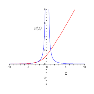
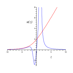
Figure 1: Comparison of the $k=1$ solutions using the standard boundary conditions with the new, rational solutions, for $\Gamma=\frac{3}{2}$ and $\Gamma=\frac{5}{2}$, (see equations (17) and equation (2.4)).

2.6 A Family of Special Solutions

It is worth noting that the $k=1$ case of $\Gamma=\frac{3}{2}$, which has $u(z)={2\nu^{2}}/{z^{2}}$, is one of an infinite family of exact solutions of this simple inverse squared form. Every $k$ has such solutions. It was already noted in ref.[6], that for $k=m$, the value $\Gamma=\frac{1}{2}+m$ yields an exact solution $u(z)=m(m+1)\nu^{2}/z^{2}$. This yields exact expressions for the free energy and partition function which are given by:

$$F = -\frac{1}{2}\left(\Gamma^{2}-\frac{1}{4}\right)\ln|\mu|=-\frac{m(m+1)}{2}\ln|\mu|\ ,$$

$$Z_{\Gamma} = |\mu|^{\frac{1}{2}\left(\Gamma^{2}-\frac{1}{4}\right)}=|\mu|^{\frac{m(m+1)}{2}}\ .$$ (32)

In fact, there are even more solutions of this form. If we index solutions by the integers $(k,m)$, meaning the $k$th model with $\Gamma=\frac{1}{2}+m$, and were to make a table of the solutions, with $m$ increasing downwards indexing rows and $k$ increasing to the right indexing columns, then the cases referred to above lie on the leading diagonal. See table 1 on page 1. Actually, the entire upper right triangle above the diagonal also contains solutions of the form, as we shall now prove.

The equation we are solving is equation (1) and we set $t_{k}$ so that ${\cal R}=cR_{k}-z$, where $c$ is a constant chosen such that the coefficient of $u^{k}$ is unity. The exception is the case $k=0$, which still has meaning here. In this case, $c$ is actually zero, and so ${\cal R}=-z$. There are nevertheless solutions for $u(z)$ since the string equation is now:

$$uz^{2}+\nu^{2}\frac{1}{4}=\nu^{2}\Gamma^{2}\ ,$$ (33)

and so we see that there is a solution $u(z)=\nu^{2}\left(\Gamma^{2}-\frac{1}{4}\right)/z^{2}=m(m+1)\nu^{2}/z^{2}$ for every $m$ at $k=0$. This is the first column in our table. The other special case of interest is the first row, $m=0$, i.e., $\Gamma=\frac{1}{2}$. For this case, the $u$–independent terms in the string equation cancel exactly, and the remaining terms vanish individually for $u=0$.

To show the existence of several more solutions of the form $u(z)=A/z^{2}$, we can proceed by differentiating the string equation once with respect to $z$. After doing this, a common factor of ${\cal R}$ can be discarded, leaving a very simple equation[3]:

$$u^{\prime}{\cal R}+2u{\cal R}^{\prime}-\frac{1}{2}{\cal R}^{\prime\prime\prime}=0\ ,$$ (34)

and substituting the form ${\cal R}=cR_{k}-z$, the recursion relation (3) for the $R_{k}$ can be used to show that

$$2cR_{k+1}^{\prime}+zu^{\prime}+2u=0\ .$$ (35)

The key point is that the last two terms cancel each other if $u(z)=A/z^{2}$ for $A$ constant. So this leaves us to determine whether $R_{k+1}^{\prime}$ can vanish. It obviously does so if $u=0$, recovering our $m=0$ family above, but there is an additional striking fact (which we shall again put to great use in later sections): For $k>m$, the differential polynomials $R_{k}$ and their derivatives vanish identically for this form of $u$ when $A=m(m+1)$. Therefore, the entire upper right triangle of solutions in table 1 (page 1) is of the exact form $u=m(m+1)\nu^{2}/z^{2}$.

For the solutions below the diagonal (and away from the $k=0$ column to the left), more intricate rational forms appear, and can be generated recursively by use of the explicit Bäcklund transformations of equation (9), as we did earlier for $k=1$. For further examples, for $k=2$ we have displayed the case of $\Gamma=\frac{7}{2}$ in table 1, and for $\Gamma=\frac{9}{2}$ we have:

$$u=\frac{20\nu^{2}z^{3}(z^{15}+168z^{10}\nu^{4}+26208z^{5}\nu^{8}-451584\nu^{12})}{(z^{10}-168z^{5}\nu^{4}-1344\nu^{8})^{2}}$$ (36)

and at $\Gamma=\frac{9}{2}$, for $k=3$:

$$u=\frac{20\nu^{2}(z^{14}+2592z^{7}\nu^{6}+155520\nu^{12})}{z^{2}(z^{7}-720\nu^{6})^{2}}$$ (37)

We list several entries in table 1, showing the overall structure of the solution space that we have uncovered. While the $k=1$ case maps to the Painlevé II equation, for which rational solutions have been uncovered in the classic work of ref.[19], the other higher $k$ cases represent a large family of interesting generalisations. Note also the fact that we have uncovered an infinite family of generalisations of the Yablonski–Vorobiev polynomials. For example, for the $k=2$, $m=3$ case, the partition function is:

$$Z=|\mu^{5}-24\nu^{4}|\ ,$$ (38)

while for $k=2$, $m=4$, it is

$$Z=|\mu^{10}-168\mu^{5}\nu^{4}-1344\nu^{8}|\ .$$ (39)

These should be compared to their $k=1$ counterparts for $m=2$ and $m=3$ in equations (2.4) and (2.4).

Table 1: The structure of the large family of rational solutions for $u(z)$ possessed by the string equation (1), for $\Gamma=\frac{1}{2}+m$.

	$k=0$	$k=1$	$k=2$	$k=3$	$k=4$	$\ldots$
$m=0$	$0$	$0$	$0$	$0$	$0$	$\ldots$
$m=1$	$\frac{2\nu^{2}}{z^{2}}$	$\frac{2\nu^{2}}{z^{2}}$	$\frac{2\nu^{2}}{z^{2}}$	$\frac{2\nu^{2}}{z^{2}}$	$\frac{2\nu^{2}}{z^{2}}$	$\ldots$
$m=2$	$\frac{6\nu^{2}}{z^{2}}$	$\frac{6\nu^{2}z(z^{3}+4\nu^{2})}{(z^{3}-2\nu^{2})^{2}}$	$\frac{6\nu^{2}}{z^{2}}$	$\frac{6\nu^{2}}{z^{2}}$	$\frac{6\nu^{2}}{z^{2}}$	$\ldots$
$m=3$	$\frac{12\nu^{2}}{z^{2}}$	$\frac{12z\nu^{2}(z^{9}+150z^{3}\nu^{4}-200\nu^{6})}{(z^{6}-10z^{3}\nu^{2}-20\nu^{4})^{2}}$	$\frac{12\nu^{2}(z^{10}+72z^{5}\nu^{4}+96\nu^{8})}{z^{2}(z^{5}-24\nu^{4})^{2}}$	$\frac{12\nu^{2}}{z^{2}}$	$\frac{12\nu^{2}}{z^{2}}$	$\ldots$
$m=4$	$\frac{20\nu^{2}}{z^{2}}$	$\mbox{equation}~{}(\ref{eq:uv92})$	equation (36)	equation (37)	$\frac{20\nu^{2}}{z^{2}}$	$\ldots$
$\vdots$	$\vdots$	$\vdots$	$\vdots$	$\vdots$	$\vdots$	$\ddots$

3 Some Spectra

As already mentioned, there is an important associated eigenvalue problem, written in equation (14). A solution at $\lambda=0$ was written in equation (30), but the nature of the solutions away from $\lambda=0$ is of interest.

It is useful to write the problem in different variables [13], defining the function $\phi(z)$ and the variable $x$ by $\psi=x^{\frac{1}{2}}\phi(x)$, $x=\lambda^{\frac{1}{2}}z/\nu$. For the potential $u$, the problem becomes:

$$x^{2}\frac{\partial^{2}\phi}{\partial x^{2}}+x\frac{\partial\phi}{\partial x}+\phi\left(x^{2}-\frac{1}{4}-\frac{x^{2}u}{\lambda}\right)=0\ ,$$ (40)

which takes a rather simple form in the large $z$ (or $x$) limit. In this limit, $u\sim\frac{\lambda}{x^{2}}\left(\Gamma^{2}-\frac{1}{4}\right)$ for all solutions. Our equation then becomes Bessel’s equation:

$$x^{2}\frac{\partial^{2}\phi}{\partial x^{2}}+x\frac{\partial\phi}{\partial x}+\left(x^{2}-\Gamma^{2}\right)\phi=0\ .$$ (41)

In general, our rational solutions for $u(z)$ define an interesting family of generalizations of Bessel’s functions (remaining asymptotic to them at large $z$ or $x$) that would be interesting to study. We will leave that for future investigations.

Recalling that there is an infinite family of special cases where $u=\frac{\lambda}{x^{2}}\left(\Gamma^{2}-\frac{1}{4}\right)$ exactly, it is especially interesting to study this exact Bessel function case. In fact, the relevant solutions are $\phi(x)=J_{\Gamma}(x)$, where:

$$J_{n}(x) = \sum_{l=0}^{\infty}\frac{(-1)^{l}}{2^{2l+|n|}l!(|n|+l)!}x^{2l+|n|}\ ,\quad|n|\neq\frac{1}{2}\ ,$$

$$J_{-\frac{1}{2}}(x) = \sqrt{\frac{2}{\pi x}}\cos x\ ,$$

$$J_{\frac{1}{2}}(x) = \sqrt{\frac{2}{\pi x}}\sin x\ ,$$ (42)

and this translates, in our original problem, to $\psi(z)=\nu^{-1/2}\lambda^{1/4}z^{1/2}J_{\Gamma}(\lambda^{1/2}z/\nu)$. This is exact for $\Gamma=\frac{1}{2}+m$ for $k\geq m$, for which the potential is $u=\lambda m(m+1)/x^{2}$. The very simplest case is $\Gamma=\frac{1}{2}$, for which the potential vanishes. Indeed, we see that the solutions are just purely sinusoidal or cosinusoidal, representing free fields.

4 On Microscopic and Macroscopic Loops

We have already seen, by examining the perturbative expansion, that our models don’t seem to contain branes. Let us explore this further. A very useful diagnostic tool in this context is the loop operator $w(\lambda,\mu)$, and its Laplace transform $w(\ell,\mu)$, which are related to ${\hat{R}}(z,\lambda)$, the diagonal of the resolvent of the Hamiltonian ${\cal H}=-\nu^{2}\partial_{z}^{2}+u(z)$:

$${\hat{R}}(z,\lambda)\equiv\langle z|\frac{1}{{\cal H}+\lambda}|z\rangle\ ,$$ (43)

as follows[9, 21]:

$$\langle w(\lambda,\mu)\rangle=\int^{\mu}{\hat{R}}(z,\lambda)dz=\int_{0}^{\ell}\langle w(\ell,\mu)\rangle e^{-\lambda\ell}d\ell\ .$$ (44)

(Note here that the $\lambda$ in the equations immediately above has the opposite sign to the $\lambda$ of the previous section. This is a matter of convention, and removes numerous factors of $(-1)^{1/2}$ in what follows.) The expectation value $\langle w(\lambda,\mu)\rangle$, once integrated once with respect to $\lambda$ and divided by $\nu$, is —when the familiar choices of section 2.2 are made— the free energy of a D–brane probe that lies along the Liouville direction, the FZZT D–brane[22, 23]. It is of course closely related to the set of eigenfunctions and eigenvalues $\{\psi_{\lambda}(z),\lambda\}$ of ${\cal H}$, which, taken together as defining a function $\psi(\mu,\lambda)=\psi(z,\lambda)|_{z=\mu}$ of $\lambda$, may be thought of as the FZZT partition function[16]. This free energy is also the effective potential $V_{\rm eff}(\lambda,\mu)$ for one scaled eigenvalue in the original matrix model language and gives information about the ZZ D–branes in the theory, as we shall discuss near the end of the next two subsections 4.1 and 4.2.

To proceed, we note that the resolvent satisfies the non–linear equation of Gel’fand and Dikii[10]:

$$4[u(z)+\lambda]{\hat{R}}^{2}-({\hat{R}}^{\prime})^{2}+2{\hat{R}}{\hat{R}}^{\prime\prime}=1\ .$$ (45)

(Recall that a prime denotes $\nu\partial/\partial z$.) Calculating $R(z,\lambda)$ for an arbitrary potential $u(z)$ is a tall order in general, but often, progress can be made via the expansion[10]:

$${\hat{R}}(z,\lambda)=\sum_{m=0}^{\infty}\frac{R_{m}[u]}{\lambda^{m+\frac{1}{2}}}\ ,$$ (46)

where the $R_{m}[u]$, differential polynomials in $u(z)$ and its derivatives, were defined above in equations (3) and (4).

One might also make sensible progress by developing ${\hat{R}}(z,\lambda)$ as a perturbative expansion in small $\nu$, corresponding essentially to the string loop expansion. From this, one can learn about the physics of loops at least order by order in string perturbation theory.

4.1 Standard Loops

For orientation, it might be helpful to first discuss the case where we have the familiar loop behaviour, in order to understand what is to come. For the case of $k=1$, with $\Gamma$ integer, we have from the large positive $z$ expansion, the leading order (sphere level) solution:

$$u(z)=z+O(\nu)\ .$$ (47)

We can see directly from the Gel’fand–Dikii equation (45) that only the first term on the left hand side survives in this limit, and pure algebra yields the result:

$${\hat{R}}(z,\lambda)=\frac{1}{2(z+\lambda)^{\frac{1}{2}}}\ .$$ (48)

Before proceeding, however, let us arrive at this by the alternative route afforded by equation (46). The Gel’fand–Dikii differential polynomials (4) for the solution (47) become:

$$R_{0}=\frac{1}{2}\ ,\quad R_{1}=-\frac{z}{4}\ ,\quad R_{2}=\frac{3}{16}z^{2}\ ,\quad R_{3}=-\frac{10}{64}z^{3}\ ,\ldots\ ,$$ (49)

(neglecting terms of order $\nu$ and higher) and so

$${\hat{R}}(z,\lambda)=\frac{1}{2\lambda^{\frac{1}{2}}}-\frac{z}{4\lambda^{\frac{3}{2}}}+\frac{3}{16}\frac{z^{2}}{\lambda^{\frac{5}{2}}}-\frac{10}{64}\frac{z^{3}}{\lambda^{\frac{7}{2}}}+\cdots\ ,$$ (50)

which, upon inspection, can be seen to be re–summed to give our expression in equation (48). From the resolvent, we can evaluate the expectation value of the loop operator:

$$\langle w(\lambda,\mu)\rangle=(\mu+\lambda)^{\frac{1}{2}}\ .$$ (51)

There are two interesting perturbative regimes, $\lambda\gg\mu$ and $\lambda\ll\mu$. The former (the integral of what was seen above) is an expansion in half integer powers of $\lambda$:

$$\langle w(\lambda,\mu)\rangle=\lambda^{\frac{1}{2}}+\frac{1}{2}\frac{\mu}{\lambda^{\frac{1}{2}}}-\frac{1}{8}\frac{\mu^{2}}{\lambda^{\frac{3}{2}}}+\frac{1}{16}\frac{\mu^{3}}{\lambda^{\frac{5}{2}}}-\frac{5}{128}\frac{\mu^{4}}{\lambda^{\frac{7}{2}}}+\cdots$$ (52)

while the other is in terms of integer powers of $\lambda$:

$$\langle w(\lambda,\mu)\rangle=\mu^{\frac{1}{2}}+\frac{1}{2}\frac{\lambda}{\mu^{\frac{1}{2}}}-\frac{1}{8}\frac{\lambda^{2}}{\mu^{\frac{3}{2}}}+\frac{1}{16}\frac{\lambda^{3}}{\mu^{\frac{5}{2}}}-\frac{5}{128}\frac{\lambda^{4}}{\mu^{\frac{7}{2}}}+\cdots$$ (53)

Now, since $\lambda$ is conjugate to loop length $\ell$ in the action of the theory, the small $\lambda$ regime should be dominated by the physics of long loop length $\ell$, and we should expect to see (if such physics is present) the exponential suppression of the amplitude $w(\ell,\mu)$ for large $\ell$, in this case $e^{-\mu\ell}$. This is clear from the full expression (51). On the other hand, the large $\lambda$ regime will be dominated by the physics of microscopic loop length $\ell$. In this regime, we find for $w(\ell,\mu)$:

$$\langle w(\ell,\mu)\rangle=\sum_{k=0}^{\infty}\frac{\ell^{k+\frac{1}{2}}}{\Gamma\left(k+\frac{1}{2}\right)}\langle{\cal O}_{k}\rangle\ ,\quad\langle{\cal O}_{0}\rangle=-\frac{\mu^{2}}{8}\ ,\langle{\cal O}_{1}\rangle=\frac{\mu^{3}}{16}\ ,\langle{\cal O}_{2}\rangle=-\frac{5\mu^{4}}{128}\ ,\ldots$$ (54)

where here, the $\Gamma$ refers to the $\Gamma$–function, not the parameter $\Gamma$. It is nice to check that this fits with some of the other things we have established about the theory’s operator content. The basic object, $u(z)$ is obtained from the free energy by differentiating twice with respect to $\mu$ (and setting $\mu=z$), and so is the two point function $\langle PP\rangle$ of the object that couples to $\mu$. The operator is sometimes called $P$, the puncture operator (at least when $k=1,2$), after the operator which measures the area of worldsheets. So we have $\langle PP\rangle=\mu$. On the other hand, we have $\langle{\cal O}_{0}\rangle=-\frac{\mu^{2}}{8}$, and so $\langle P{\cal O}_{0}\rangle=-\mu/4$. But since $t_{0}=-4\mu$, we have $\langle P\dots\rangle=-\frac{1}{4}\langle{\cal O}_{0}\cdots\rangle$, and so we recover that $u=\langle PP\rangle=\mu$. For the operator ${\cal O}_{1}$, we have the KdV flows of equation (6). An insertion of ${\cal O}_{1}$ is differentiation with respect to $t_{1}$. We can do this in the presence to two insertions of $P$, in which case the KdV flows tell us that since $R_{2}=3\mu^{2}/16$, we have $\langle PP{\cal O}_{1}\rangle=\frac{3}{8}\mu$. Integrating twice with respect to $\mu$ we confirm that $\langle{\cal O}_{1}\rangle=\frac{\mu^{3}}{16}$. This can be checked for $\langle{\cal O}_{2}\rangle$ and so on.

In this way, we see that the microscopic loops that arise in the large $\lambda$ regime are nothing but the insertions of the point–like operators corresponding to the closed string sector, as is well known[12]. We can write the expectation value of the operators as:

$$<{\cal O}_{k}>=\int^{\mu}\!\!R_{k+1}[u(z)]\,\,dz\ .$$ (55)

Another useful piece of physics that can be extracted from this probe is the presence and action of point–like D–branes in the theory. The loop expectation value in equation (51) can be integrated once with respect to $\lambda$, and after dividing by $\nu$ the result gives the effective potential $V_{\rm eff}(\lambda,\mu)$ for one scaled eigenvalue in the original matrix model language. The potential’s extrema (where $\langle w(\lambda,\mu)\rangle$ vanishes) correspond to the presence of ZZ D–branes, as seen by our probe. The value of the potential at the extremum gives the action/tension of the brane[24, 25]. In the current example, we can see that $\langle w(\lambda,\mu)\rangle$ vanishes at finite $\lambda$, and the resulting brane tension is proportional to $\mu^{\frac{3}{2}}/\nu$, which from equation (8) tells us that the tension is of order $g_{s}^{-1}$, as it should be for a D–brane.

Let us now turn to the models in question. We need to compute the resolvent in this case, using much more complicated expressions for the function $u(z)$. Given what has gone before, one might hope that for these rational solutions, some special circumstance might transpire that may well render the problem more tractable. One might expect, for example, that once again the expansion of equation (46) in inverse powers of $\lambda^{\frac{1}{2}}$ becomes re–summable into a closed form solution, as happened for the example above. In fact, the result is even prettier than that, as we shall see.

4.2 New Loops: The Special Solutions

Let us start with the simplest solutions, the special family of exact solutions identified earlier,

$$u(z)=\frac{\nu^{2}\left(\Gamma^{2}-\frac{1}{4}\right)}{z^{2}}=\frac{m(m+1)\nu^{2}}{z^{2}}\ ,\quad k\geq m,\quad\Gamma=\frac{1}{2}+m\ ,$$ (56)

In fact, for these, there is a spectacular simplification. For this form, the Gel’fand–Dikii differential polynomials $R_{k}[u]$, equation (4), actually vanish identically for $k>m$. For example, for $\Gamma=\frac{1}{2}$ we have that $u=0$, and therefore the only non–vanishing differential polynomial is the trivial one, $R_{0}=\frac{1}{2}$. For $\Gamma=\frac{3}{2}$, we have

$$u=\frac{2\nu^{2}}{z^{2}}\ ,\quad R_{0}=\frac{1}{2}\ ,\quad R_{1}=-\frac{1}{2}\frac{\nu^{2}}{z^{2}}\ ,$$ (57)

and the other $R_{k}[u]$ identically vanish. For $\Gamma=\frac{5}{2}$, we have

$$u=\frac{6\nu^{2}}{z^{2}}\ ,\quad R_{0}=\frac{1}{2}\ ,\quad R_{1}=-\frac{3\nu^{2}}{2z^{2}}\ ,\quad R_{2}=\frac{9\nu^{4}}{2z^{4}}\ ,$$ (58)

with all other $R_{k}[u]$ vanishing, and finally for $\Gamma=\frac{7}{2}$, we have

$$u=\frac{12\nu^{2}}{z^{2}}\ ,\quad R_{0}=\frac{1}{2}\ ,\quad R_{1}=-\frac{3\nu^{2}}{z^{2}}\ ,\quad R_{2}=\frac{45\nu^{4}}{2z^{4}}\ ,\quad R_{3}=-\frac{225\nu^{6}}{2z^{6}}\ ,$$ (59)

with all other $R_{k}[u]$ vanishing. This means that in the case of the special solutions, the expression for the resolvent is exact, starting at order $\lambda^{-1/2}$ and ending at order $\lambda^{-\Gamma}$, with precisely $\Gamma+\frac{1}{2}=m+1$ terms, for example:

$$\Gamma = \frac{1}{2}\ ,\quad{\hat{R}}(z,\lambda)=\frac{1}{2\lambda^{\frac{1}{2}}}$$

$$\Gamma = \frac{3}{2}\ ,\quad{\hat{R}}(z,\lambda)=\frac{1}{2\lambda^{\frac{1}{2}}}\left(1-\frac{\nu^{2}}{z^{2}\lambda}\right)$$

$$\Gamma = \frac{5}{2}\ ,\quad{\hat{R}}(z,\lambda)=\frac{1}{2\lambda^{\frac{1}{2}}}\left(1-\frac{3\nu^{2}}{z^{2}\lambda}+\frac{9\nu^{4}}{z^{4}\lambda^{2}}\right)$$

$$\Gamma = \frac{7}{2}\ ,\quad{\hat{R}}(z,\lambda)=\frac{1}{2\lambda^{\frac{1}{2}}}\left(1-\frac{6\nu^{2}}{z^{2}\lambda}+\frac{45\nu^{4}}{z^{4}\lambda^{2}}-\frac{225\nu^{6}}{z^{6}\lambda^{3}}\right)\ .$$ (60)

Now we can integrate once with respect to $z$ to get the loop operator $w(\lambda,\mu)$. For example:

$$\Gamma = \frac{1}{2}\ ,\quad\langle w(\lambda,\mu)\rangle=\frac{\mu}{2\lambda^{\frac{1}{2}}}$$

$$\Gamma = \frac{3}{2}\ ,\quad\langle w(\lambda,\mu)\rangle=\frac{\mu}{2\lambda^{\frac{1}{2}}}\left(1+\frac{\nu^{2}}{\mu^{2}\lambda}\right)$$

$$\Gamma = \frac{5}{2}\ ,\quad\langle w(\lambda,\mu)\rangle=\frac{\mu}{2\lambda^{\frac{1}{2}}}\left(1+\frac{3\nu^{2}}{\mu^{2}\lambda}-\frac{3\nu^{4}}{\mu^{4}\lambda^{2}}\right)$$

$$\Gamma = \frac{7}{2}\ ,\quad\langle w(\lambda,\mu)\rangle=\frac{\mu}{2\lambda^{\frac{1}{2}}}\left(1+\frac{6\nu^{2}}{\mu^{2}\lambda}-\frac{15\nu^{4}}{\mu^{4}\lambda^{2}}+\frac{45\nu^{6}}{\mu^{6}\lambda^{3}}\right)\ .$$ (61)

and here we must remember that these are exact expressions for models $m=0,1,2,3,$ respectively (recall that the inverse squared potential is exact for the $k$th model when $\Gamma=\frac{1}{2}+m$, with $k\geq m$.)

There are a number of remarks to be made here. The first is that we have a finite number of terms in these exact $\lambda$ expansions, and also in the corresponding $\ell$ expansions in the Laplace transforms. So looking at the large $\lambda$ limit, which is dominated by the physics of small $\ell$ loops, we have only a finite number of operators ${\cal O}_{j}$ appearing in the theory, the values $j=0,\ldots,m-1$ for $\Gamma=\frac{1}{2}+m$, and so far we have $k\geq m$. The second remark is that while our loop has a small $\ell$ (large $\lambda$) expansion of a sort similar to the usual behaviour discussed above, the large $\ell$ (small $\lambda$) regime is very different. There is no re–summation of the series (since it is of a finite number of terms) into an expression that at small $\lambda$ supports the characteristic $e^{-\mu\ell}$ behaviour. In other words, the theory does not possess the large loop FZZT D–brane physics seen before.

The same features are responsible for the absence of point–like ZZ D–branes from the picture painted by our probe as well. The extrema of the effective potential $V_{\rm eff}(\lambda,\mu)=\nu^{-1}\int\langle w(\lambda,\mu)\rangle d\lambda$, given by the zeros of the loop operator, are located where $\lambda$ goes to infinity. So if there were ZZ D–branes present, they would be located by our probe as being in the weak coupling regime in the Liouville direction $\varphi=-\ln\lambda$, but an evaluation of the effective potential there gives an infinite result. Again, an infinite number of terms in the $\lambda^{-1/2}$ expansion are needed allow the loop to have a zero at finite $\lambda$, and a corresponding finite effective potential. Such terms are not available in these models because of the remarkable truncation of the $R_{k}[u]$, and so we see that we have no ZZ D–branes. We will return to this in the conclusion section 7.

4.3 New Loops: The More General Solutions

Having seen the remarkable simplifications that occurred in the last subsection, for the special solutions $u=m(m+1)\nu^{2}/z^{2}$, let us turn to the more general rational solutions that occur for $\Gamma=\frac{1}{2}+m$ with $k<m$. Focusing on $k=1$ for definiteness, let us look at $\Gamma=\frac{5}{2}$. The potential is given in equation (2.4), and proceeding to evaluate the Gel’fand–Dikii polynomials, it is a remarkable surprise to find that once again they vanish beyond a certain order. This time, it is for order beyond two. This matches the previous pattern: Recall that for $\Gamma=\frac{1}{2}+m$, the $R_{k}$ for $k>m$ vanished, for the special solutions. In fact, it happens again here, even for these much more complicated rational solutions. This is the general pattern.

In this $m=2$ example, we have:

$$R_{0}=\frac{1}{2}\ ;\quad R_{1}=-\frac{3z\nu^{2}(z^{3}+4\nu^{2})}{2(z^{3}-2\nu^{2})^{2}}\ ;\quad R_{2}=\frac{9\nu^{4}z^{2}}{2(z^{3}-2\nu^{2})^{2}}\ ,$$ (62)

with all other $R_{k}$ vanishing. The resolvent is then:

$${\hat{R}}(z,\lambda)=\frac{1}{2\lambda^{\frac{1}{2}}}\left(1-\frac{3z(z^{3}+4\nu^{2})}{(z^{3}-2\nu^{2})^{2}}\frac{\nu^{2}}{\lambda}+\frac{9z^{2}}{(z^{3}-2\nu^{2})^{2}}\frac{\nu^{4}}{\lambda^{2}}\right)\ ,$$ (63)

with an expression for the loop that is:

$$\langle w(\lambda,\mu)\rangle=\frac{\mu}{\lambda^{\frac{1}{2}}}+\frac{3\mu^{2}}{2(\mu^{3}-2\nu^{2})^{2}}\frac{\nu^{2}}{\lambda^{\frac{3}{2}}}-\frac{3}{2(\mu^{3}-2\nu^{2})^{2}}\frac{\nu^{4}}{\lambda^{\frac{5}{2}}}\ ,$$ (64)

together with its Laplace transform:

$$\langle w(\ell,\mu)\rangle=\frac{1}{\sqrt{\pi}}\left(\frac{\mu}{2\ell^{\frac{1}{2}}}+\frac{3\mu^{2}\nu^{2}\ell^{\frac{1}{2}}}{(\mu^{3}-2\nu^{2})^{2}}-\frac{2\nu^{4}\ell^{\frac{3}{2}}}{(\mu^{3}-2\nu^{2})^{2}}\right)\ ,$$ (65)

showing the appearance of a finite number of point–like (closed string) operators, as before.

$$\langle{\cal O}_{0}\rangle=\frac{3\mu^{2}\nu^{2}}{(\mu^{3}-2\nu^{2})^{2}}\ ;\quad\langle{\cal O}_{1}\rangle=-\frac{3\nu^{4}}{2(\mu^{3}-2\nu^{2})^{2}}\ .$$ (66)

5 Point–Like Operators

So we’ve established from the previous section that we have indeed a family of point–like operators organised by the KdV flows, as is familiar for the case of $\Gamma$ integer, or in the bosonic string.

There is a major difference in how the operator content manifests itself in this situation, however, and it is worth pausing to appreciate it. In the standard theories, there is an infinite set of operators ${\cal O}_{k}$, for which the KdV flows describe the insertion:

$$\langle{\cal O}_{0}{\cal O}_{0}{\cal O}_{k}\rangle\equiv\frac{\partial u}{\partial t_{k}}=R_{k+1}^{\prime}[u]\ .$$ (67)

The Virasoro constraints (loop equations for microscopic loops) remove[26] an infinite set of these operators from the system, by supplying a set of recursion relations between correlation functions of the ${\cal O}_{k}$. These relations can be used to eliminate an infinite set of operators, leaving only a physical set: For the $k$th model, only the operators ${\cal O}_{0}\cdots{\cal O}_{k-1}$ survive.

In our case, things are much simpler. For a given model, the $k$th, turning on some $\Gamma=\frac{1}{2}+m$ ($m>k$) has the remarkable result of removing the effects of all operators ${\cal O}_{j}$ for $j>m$. This is consistent with the structure of table 1 (page 1), and follows from our observation that the $R_{j+1}$ vanish for $j>m$. This is before the action of the Virasoro constraints which presumably reduces the operator content back to only ${\cal O}_{0}\cdots{\cal O}_{k-1}$, for this $k$th model.

In the case of the $k$th model, switching on instead $k$ units (i.e., setting $m=k$) reduces the model to $u=m(m+1)\nu^{2}/z^{2}$, (we are on the diagonal of table 1) and the operator content is precisely the minimal set ${\cal O}_{0}\cdots{\cal O}_{k-1}$ with no appeal to Virasoro.

If instead for the $k$th model we have $m<k$, then we are in the upper right triangle of table 1 and the potential is still $u=m(m+1)\nu^{2}/z^{2}$, and there are at most $m$ operators: ${\cal O}_{0}\cdots{\cal O}_{m-1}$. The extreme case of this is of course $m=0$. There we see, that regardless of the value of $k$, the model is controlled by the completely trivial potential $u=0$. There is no operator content. This will all play a role in our interpretive discussion in the conclusions section 7.

6 Phase Transitions

An unusual feature of our models is the existence of points on the real $\mu$ line where the partition function vanishes. See figure 2 for $k=1$ examples $\Gamma=\frac{5}{2},\frac{7}{2}$. At such points, the free energy goes through a discontinuity, and there are poles in all correlation functions of point–like operators.

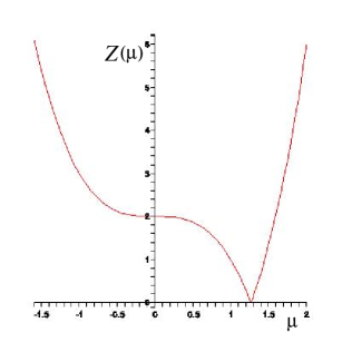
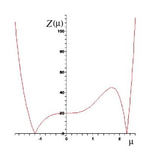
Figure 2: The partition function $Z(\mu)$ as a function of $\mu$ for the $k=1$ cases of $\Gamma=\frac{5}{2}$ and $\frac{7}{2}$. There is a phase transition whenever there is a zero.

A zero of the partition function has its origins in a double pole of $u(z)$. The appearance of a double pole in the function $u(z)$ has been considered before, in the context of the non–perturbative physics uncovered in the original double scaling limit of refs.[7, 8, 9]. The accompanying physics was originally conjectured[7, 12] to be indicative of a phase transition, but this idea was left undeveloped as the discussion was overtaken by other more pressing physical issues. Among them were:

1. The controlling string equation was not our equation (1), but instead Painlevé I:

   $$-\frac{\nu^{2}}{3}\frac{\partial^{2}u(z)}{\partial z^{2}}+u^{2}=z\ ,$$ (68)

   with a large $z$ asymptotic $u\sim z^{1/2}+O(\nu)$. For a real solution with that asymptotic, there is an infinite number of double poles on the real axis, and the location of the first such pole in not fixed by perturbation theory. So there is a non-perturbative parameter corresponding to the location, $z_{0}$ of the first pole.

2. With a pole in $z$, and the above asymptotic, there is inevitably only a discrete spectrum for the Hamiltonian ${\cal H}$. This discrete spectrum, with eigenvalues $\lambda_{i}$, gives poles in $\lambda$ in the loop $\langle w(\lambda)\rangle$, which non–perturbatively violate[27, 28] the loop equations for $\langle w(\lambda)\rangle$.

In our case, we avoid these issues neatly, since:

1. The physics supplies us with a different string equation, given by equation (1), and different solutions. The locations of the poles of our rational functions are fixed. There are no non–perturbative parameters to be determined. Let us denote the location of the first pole coming from $z=+\infty$ as $z_{0}$. It is a fully determined quantity.

2. There is always a continuous spectrum on $(z_{0},+\infty)$, given by our studies in section 3, the wavefunctions being Bessel functions for the special solutions, and asymptotically so for the general case. There are therefore no $\lambda$–poles in the loop $w(\lambda)$, and from the modern perspective, this ensures that the Liouville coordinate (at least as seen by this probe), $\varphi=-\ln\lambda$, is continuous. There is of course a discrete spectrum that must arise between two successive poles, for rational solutions for which there are multiple $z$–poles. Perhaps those are disconnected regions upon which we do not consider our physics. We need not do so since our wavefunctions vanish at the boundaries of these regions and so there can be no tunneling. Logically, it is possible that an examination of the loop equations for these models may yield consistent physics for those regimes as well. There is the intriguing possibility that these regimes represent physics where these probes see the Liouville direction $\varphi$ as having fractionated into discrete points. This is a subject for future study.

So now that we have a very well-behaved system, we are free to re-examine the meaning of the transitions at the zeros of $Z(\mu)$. At present, it is not at all clear what the physical interpretation of the transition is, and whether earlier speculations[7, 12] about this being a “condensation of handles” are relevant here. This seems unlikely here (although there may be surprises), given that one of the hallmarks of our physics seems to be the very gentle growth of genus perturbation theory. So we might look elsewhere for an interpretation, and have not yet found one.

It is interesting to note some general properties of the transition. Essentially, the properties of the partition function in the neighbourhood of the zeros is captured by the special solutions $u=m(m+1)\nu^{2}/z^{2}$, and so we can focus on them. Recall that the partition function is $Z(\mu)=|\mu|^{\frac{m(m+1)}{2}}$, and so except for the case of $m=1$, its first $\mu$–derivative at the transition vanishes. For $m=1$, it has a jump discontinuity from $-1$ to $+1$. The quantity $\partial Z/\partial\mu$ may therefore be part of a definition of a useful order parameter. The natural quantity for all $m$ might in fact be $\mu(\partial Z/\partial\mu)$ since it vanishes at the transition point for all $m$. We will leave the study of these transitions for future work, but expect that the properties above will play an important role in characterising the physics.

7 Conclusion

A useful way to restate some of our key results seems to be as follows. For integer $\Gamma$ we know that this regime represents background R–R flux, which can be described in the worldsheet theory in terms of insertions of a closed string operator into all correllators, etc. For half integer $\Gamma=\frac{1}{2}+m$, ($m\in{}^{+}$), we still have an expansion in terms of closed string world sheets, and it seems economical to think of $\Gamma$ as representing an aspect of a background in the closed string theory (although it might be premature to think of it as simply half–integer R–R flux before further comparison with an explicit computation from the continuum formulation). Setting $\Gamma=\frac{1}{2}$ results in only $u=0$ as the solution to the string equation. All operators are trivial, and the theory has no content. One can therefore think of the $\Gamma=\frac{1}{2}$ background as simply screening the effects of all operators in the theory, rendering it trivial. Switching on $m$ has the interesting effect that it allows (or unscreens) $m$ operators, ${\cal O}_{0},\cdots,{\cal O}_{m-1}$, yielding non-trivial physics.

Interestingly, the theory cannot support D–branes however, since the probe of their presence —the loop operator $w(\lambda,\mu)$— needs an infinite number of the ${\cal O}_{j}$ operators to be non–zero in its large $\lambda$ expansion, so that it can be re–summed to reconstruct the required small $\lambda$ (large loop length $\ell$) behavior. These are simply not available at finite $m$.

From this perspective we can see how (at least formally) to return to the types of string theory we are familiar with. We take a large $m$ limit. In such a limit, where we can indeed fill out the expansion of the loop operator and allow it to support large loops. The presence of so many more of these operators presumably will also increase the rate of growth of string perturbation theory so that there are $\exp(-C/g_{s})$ effects again, signalling the presence of D–branes[1]. This will make sense at the level of solutions to the string equation too, and one would expect that the terms in the expansion of the function $u(z)$ will return to the form we are familiar with for integer $\Gamma$, (see equation (31)), and we can match on to the regime containing background D–branes. This would be interesting to study.

This family of models therefore represents a rather clear example of the contrast between the types of string theories that most are familiar with (with asymptotic expansions in small $g_{s}$, and branes) and this new type of model which clearly is very simple (re–summable expansions and no branes) but nonetheless, we submit, an instructive type of string theory. We’ve been able to identify aspects of the path that connects these, by explicitly following the operator content.

This may be more than an exercise for its own sake. There may well be situations involving the types of string theory we wish to use for other applications (including perhaps the study of Nature) where the background (an exotic choice of flux, perhaps) induces the type of behaviour in these models. Such models may therefore furnish an effective description of some important physical subsector of other stringy scenarios.

References

- [1] S. H. Shenker, “The Strength of nonperturbative effects in string theory,”. Presented at the Cargese Workshop on Random Surfaces, Quantum Gravity and Strings, Cargese, France, May 28 - Jun 1, 1990.
- [2] S. Dalley, C. V. Johnson, and T. Morris, “Multicritical complex matrix models and nonperturbative 2-D quantum gravity,” Nucl. Phys. B368 (1992) 625–654.
- [3] S. Dalley, C. V. Johnson, and T. Morris, “Nonperturbative two-dimensional quantum gravity,” Nucl. Phys. B368 (1992) 655–670.
- [4] S. Dalley, C. V. Johnson, and T. Morris, “Nonperturbative two-dimensional quantum gravity, again,” Nucl. Phys. Proc. Suppl. 25A (1992) 87–91, hep-th/9108016.
- [5] S. Dalley, C. V. Johnson, T. R. Morris, and A. Wätterstam, “Unitary matrix models and 2-D quantum gravity,” Mod. Phys. Lett. A7 (1992) 2753–2762, hep-th/9206060.
- [6] C. V. Johnson, “Tachyon condensation, open-closed duality, resolvents, and minimal bosonic and type 0 strings,” JHEP 12 (2004) 072, hep-th/0408049.
- [7] E. Brezin and V. A. Kazakov, “Exactly Solvable Field Theories Of Closed Strings,” Phys. Lett. B236 (1990) 144–150.
- [8] M. R. Douglas and S. H. Shenker, “Strings In Less Than One-Dimension,” Nucl. Phys. B335 (1990) 635.
- [9] D. J. Gross and A. A. Migdal, “Nonperturbative Two-Dimensional Quantum Gravity,” Phys. Rev. Lett. 64 (1990) 127.
- [10] I. M. Gel’fand and L. A. Dikii, “Asymptotic behavior of the resolvent of Sturm-Liouville equations and the algebra of the Korteweg-De Vries equations,” Russ. Math. Surveys 30 (1975) 77–113.
- [11] M. R. Douglas, “Strings In Less Than One-Dimension And The Generalized K-D- V Hierarchies,” Phys. Lett. B238 (1990) 176.
- [12] T. Banks, M. R. Douglas, N. Seiberg, and S. H. Shenker, “Microscopic And Macroscopic Loops In Nonperturbative Two- Dimensional Gravity,” Phys. Lett. B238 (1990) 279.
- [13] J. E. Carlisle, C. V. Johnson, and J. S. Pennington, “D-branes and fluxes in supersymmetric quantum mechanics,” hep-th/0511002.
- [14] J. E. Carlisle, C. V. Johnson, and J. S. Pennington, “Bäcklund transformations, D-branes, and fluxes in minimal type 0 strings,” hep-th/0501006.
- [15] C. V. Johnson, T. R. Morris, and A. Wätterstam, “Global KdV flows and stable 2-D quantum gravity,” Phys. Lett. B291 (1992) 11–18, hep-th/9205056.
- [16] I. R. Klebanov, J. M. Maldacena, and N. Seiberg, “Unitary and complex matrix models as 1-d type 0 strings,” Commun. Math. Phys. 252 (2004) 275–323, hep-th/0309168.
- [17] A. B. Zamolodchikov and A. B. Zamolodchikov, “Liouville field theory on a pseudosphere,” hep-th/0101152.
- [18] R. Gopakumar and C. Vafa, “On the gauge theory/geometry correspondence,” Adv. Theor. Math. Phys. 3 (1999) 1415–1443, hep-th/9811131.
- [19] H. Airault, “Rational solutions of Painleve equations,” Studies in Applied Mathematics 61 (July, 1979) 31–53.
- [20] M. Noumi, “Painlevé Equations Through Symmetry,” American Mathematical Society (2004) (2004).
- [21] D. J. Gross and A. A. Migdal, “A Nonperturbative Treatment Of Two-Dimensional Quantum Gravity,” Nucl. Phys. B340 (1990) 333–365.
- [22] V. Fateev, A. B. Zamolodchikov, and A. B. Zamolodchikov, “Boundary Liouville field theory. I: Boundary state and boundary two-point function,” hep-th/0001012.
- [23] J. Teschner, “Remarks on Liouville theory with boundary,” hep-th/0009138.
- [24] J. McGreevy and H. L. Verlinde, “Strings from tachyons: The c = 1 matrix reloaded,” JHEP 12 (2003) 054, hep-th/0304224.
- [25] J. McGreevy, J. Teschner, and H. L. Verlinde, “Classical and quantum D-branes in 2D string theory,” JHEP 01 (2004) 039, hep-th/0305194.
- [26] R. Dijkgraaf, H. L. Verlinde, and E. P. Verlinde, “Loop equations and Virasoro constraints in nonperturbative 2-D quantum gravity,” Nucl. Phys. B348 (1991) 435–456.
- [27] F. David, “Loop Equations And Nonperturbative Effects In Two- Dimensional Quantum Gravity,” Mod. Phys. Lett. A5 (1990) 1019–1030.
- [28] F. David, “Phases of the large N matrix model and nonperturbative effects in 2-d gravity,” Nucl. Phys. B348 (1991) 507–524.